Optimal Matching of Flapping Hydrofoil Propulsion Performance Considering Interaction Effects of Motion Parameters

Abstract

In order to maximize the propulsion efficiency of flapping hydrofoil, a new method is proposed in this paper. The effects of heave amplitude, pitch amplitude, and the phase difference between heave and surge on propulsion performance were analyzed by numerical calculation, and it was found that three motion parameters had interactive effects on flapping hydrofoil propulsion performance. BP neural network was used to fit the three motion parameters and propulsion performance. Using this function model, the optimal motion parameters can be obtained under certain thrust. In this study, the optimization matching under certain thrust was carried out by using this method, and the propulsion efficiency was improved by 7.73%.

1. Introduction

The development of underwater gliders and UUV has attracted a lot of research in recent years. Inspired by the fact that aquatic animals in nature disturb the water flow by waving their wing-like limbs to obtain lift and thrust [1]. Some people use this feature to harvest energy from the heave force of flapping hydrofoil and improve the efficiency of energy harvesting by changing the parameters of the hydrofoil flapping [2,3]. Others use the thrust of hydrofoil flapping for underwater vehicle research; people have studied the effect of the vertical reciprocating motion of hydrofoils through numerical and experimental methods, mostly focusing on the combination of pitch and heave motions. The behavior of animal flapping hydrofoil is not just a combination of simple pitching and heave motion, but usually adds a linear motion in the horizontal direction to help improve propulsion performance. There is no doubt that such a movement pattern can be applied to underwater vehicles [4].

Previous studies on flapping hydrofoil performance have carried out a significant amount of research on its propulsion performance through experiments and numerical simulations. Some papers mainly research the effect of changing the state of the flow field on propulsion performance. Techet [5] used the water tunnel experiment to analyze the changes in the thrust coefficient and propulsion efficiency by changing the pitching angle of attack and the Strouhal number. It was found that at low angles of attack, at a sufficiently high Strouhal number, higher thrust and efficiency can be obtained. Through numerical simulation, Ashraf [6] studied the effect of different airfoil thicknesses and radians on the propulsion performance of the combined pitch and heave motion at different Reynolds number. He found that with the increase in Reynolds number, choosing a thicker airfoil is beneficial to the propulsion performance of the flapping hydrofoil, and observed that the leading-edge vortex plays a key role in the propulsion performance of the flapping hydrofoil. Read [7] conducted an experimental study on the heave and pitch motion foils to obtain the optimal parameter combination of pitch angle, heave and pitch motion phase difference, and Strouhal number [8]. The best efficiency of the slice is 50–60%, and the propulsion performance is the best when the phase difference between heave and pitch motion is 90–100°. Triantafyllou et al. [9]. studied the Strouhal number on the propulsion of flapping hydrofoil, and they believed that the Strouhal number under the optimal propulsion combination of flapping hydrofoil was between 0.2 and 0.35, similar to that of aquatic organisms. Yu et al. [10] used numerical simulation to set different frequencies, maximum pitch angles, and amplitudes of flapping hydrofoil to explore the relationship between frequency and motion parameters. The efficiency is higher at high frequencies and heave amplitudes, and the low-efficiency region disappears as the pitch amplitude increases.

In the past, research on motion trajectories have mostly focused on the combined pitch and heave motion. Esfahani’s [11] research found that adding a reciprocating horizontal motion to the pitch and heave motion makes its trajectory into an ellipse, changes its effective angle of attack profile, and subsequently changes the vortex shedding pattern and wake area of the trailing edge of the wing, which significantly improves the propulsion performance of the flapping hydrofoil. Subsequently, Chen et al. [12] studied the propulsion performance of different elliptical motion trajectories of the flapping hydrofoil and gave a set of motion parameters with excellent propulsion performance by changing the ratio of the maximum amplitude of the heave motion to the horizontal motion and its phase difference.

Recently, Yang et al. [13] proposed the “8”-shaped motion trajectory and proposed that increasing the surge motion can generate multiple vortices and the resulting vortices help improve thrust. Zhang et al. [14] proposed the “∞” motion trajectory, which is considered to have the advantages of multiple thrust peaks, average thrust, and high propulsion efficiency compared with elliptical motion trajectories and “8”-shaped motion trajectories. However, the conclusion it draws is based on a pitch value of 45° and there is a lack of research and verification for the case of small pitch amplitude.

Based on the DIRECT (rectangular segmentation) global optimization algorithm, Wu et al. [15] optimized the flapping motion parameters iteratively with the specific optimization objective of maximizing the propulsion efficiency. In addition, some scholars have studied the clustering behavior of flapping hydrofoil in nature and analyzed the influence of motion parameters such as pitch amplitude and heave amplitude during the clustering of flapping hydrofoils [16].

Different from previous studies on the influence of a single parameter of flapping hydrofoil motion trajectory on the propulsion performance, this paper comprehensively considers the influence of three motion parameters, namely, heave amplitude, pitch amplitude, surge and heave difference, on the propulsion performance of flapping hydrofoil, and considered their interaction effect on the propulsion performance. In order to obtain the motion parameter combination with excellent propulsive performance, the fitting function between the motion parameters and the propulsion performance was established, and the optimal motion model with the highest propulsion efficiency under certain thrust was predicted. This work will provide guidance for the trajectory design of underwater gliders and UUV.

2. Materials and Methods

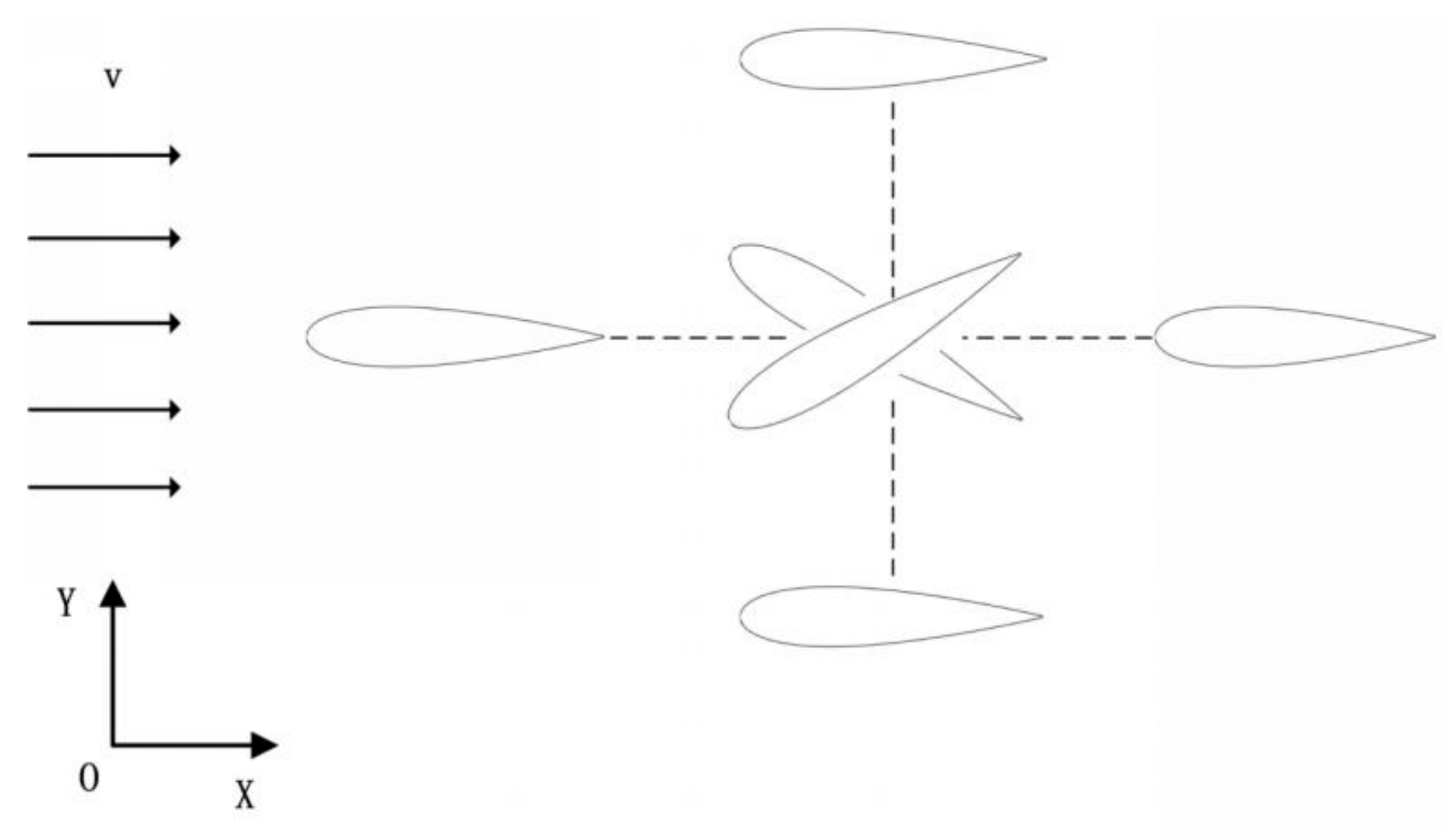
2.1. Motion Trajectory

The motion of the flapping hydrofoil consists of a reciprocating motion in the horizontal direction, the vertical direction, and a pitching motion that rotates around the pitch axis. The three motion equations are shown by Equations (1)–(3).

$$x\left(t\right)=x_0\sin \left(\omega t+\varphi \right)$$

(1)

$$h\left(t\right)=h_0\sin \left(\omega t\right)$$

(2)

$$\theta \left(t\right)={\theta }_0\sin \left(\omega t+\phi \right)$$

(3)

In this study, by changing the heave amplitude and maximum pitch angle, as well as the phase difference between the surge and heave, the effects of these motion parameters on the propulsion performance of the flapping hydrofoil were investigated. A NACA0012 hydrofoil with a chord c of 0.1m is placed in two-dimensional turbulent flow, and executes synchronous periodic heave, pitch rotary motion, and added surge motion. To simulate the real motion of the underwater vehicle as much as possible, the Reynolds number is set to 40,000, and the pitch axis is set to be at one-third of the chord length. To ensure eximious propulsion performance in this study as much as possible, the phase difference between pitch and heave motion ϕ = 90° is determined [17]. Additionally, according to the previous research, the ratio of heave amplitude to surge amplitude is determined to be 2 and the motion frequency is selected as f = 0.8 Hz. According to the conclusion given by Chen et al. [12], when the ratio of heave amplitude to surge amplitude is equal to 2, the phase difference between surge and heave motion (φ) in the range of 60° to 120° can effectively improve the propulsion performance. Next, we determined the phase difference between heave and surge motion(φ) within the range of 60–120° and selected 15° as the interval to divide into five different phase differences. The range of heave amplitude(h₀) is 0.5c~c, and the interval difference is 0.125c; the pitch amplitude(θ₀) range is 10–30°, and the interval difference is 5° [18]. According to the selection of the above experimental parameters, a total of 125 sets of numerical simulation calculations were carried out in this study.

As shown in Figure 1, the motion of the flapping hydrofoil is composed of three sub-motions, and there are five motion trajectories according to different phase differences. Figure 2 shows the five motion trajectories involved in this research.

2.2. Governing Equation and Parameter Definition

This study is based on the two-dimensional Navier–Stokes equation to calculate the incompressible viscous flow around the NACA0012 hydrofoil. According to Young’s research [19], there is little difference between laminar and turbulent models when calculating flapping hydrofoil. The governing equation are as follows:

$$\rho \left(\frac{\partial u}{\partial t}+\frac{u\partial u}{\partial x}+\frac{v\partial u}{\partial y}\right)=\mu \left(\frac{{\partial }^{2}u}{\partial x^2}+\frac{{\partial }^{2}u}{\partial y^2}\right)-\frac{\partial p}{\partial x}$$

(4)

$$\rho \left(\frac{\partial u}{\partial t}+\frac{u\partial u}{\partial x}+\frac{v\partial u}{\partial y}\right)=\mu \left(\frac{{\partial }^{2}u}{\partial x^2}+\frac{{\partial }^{2}u}{\partial y^2}\right)-\frac{\partial p}{\partial y}$$

(5)

where u and v represent the flow velocity in the x and y directions, respectively, p represents the pressure, u represents the viscosity, and ρ represents the flow density.

According to the mechanical data (thrust, lift, and moment) monitored in the Fluent software, the obtained thrust, lift and torque are dimensionless as C_t, C_l, C_m and the propulsion performance is judged according to these parameters. The definition of C_t, C_l, C_m is given below [20].

$$C_t=\frac{F_x\left(t\right)}{0.5\rho v^{2}c}$$

(6)

$$C_l=\frac{F_y\left(t\right)}{0.5\rho v^{2}c}$$

(7)

$$C_m=\frac{M\left(t\right)}{0.5\rho v^2{c}^2}$$

(8)

The input power of the flapping hydrofoil can be defined based on the measured mechanical data.

$$P_I\left(t\right)=\frac{F_x\left(t\right)\cdot dx\left(t\right)}{dt}+\frac{F_y\left(t\right)\cdot dh\left(t\right)}{dt}+\frac{M\left(t\right)\cdot d\theta \left(t\right)}{dt}$$

(9)

The input power P_I can be further defined in dimensionless form as:

$$C_P=\frac{C_{t}d{v}_x+C_{l}d{v}_y+C_m\mathrm{c}d{v}_{\theta }}{Vdt}$$

(10)

Define the average input efficiency and average thrust coefficient over a period.

$$\overline{C_t}=\frac{{\displaystyle \int {}_0^T{F}_x(t)dt}}{0.5T\rho v^{2}c}$$

(11)

$$\overline{C_p}=\frac{{\displaystyle \int {}_0^T{P}_I(t)dt}}{0.5T\rho v^{2}c}$$

(12)

The propulsion efficiency of a flapping hydrofoil is defined as follows:

$$\eta =\frac{\overline{C_t}}{\overline{C_P}}$$

(13)

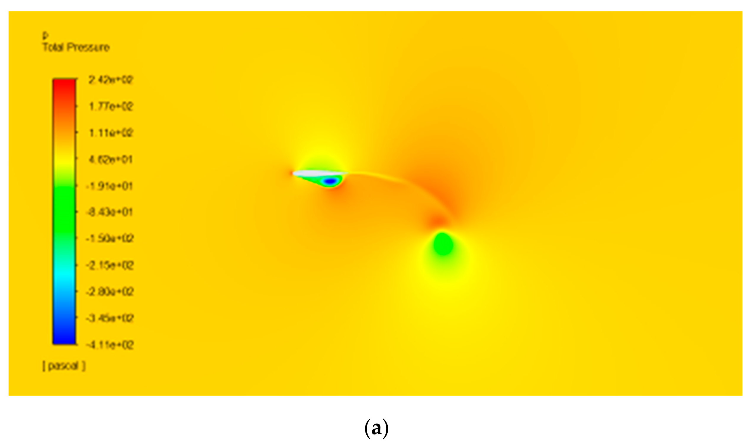
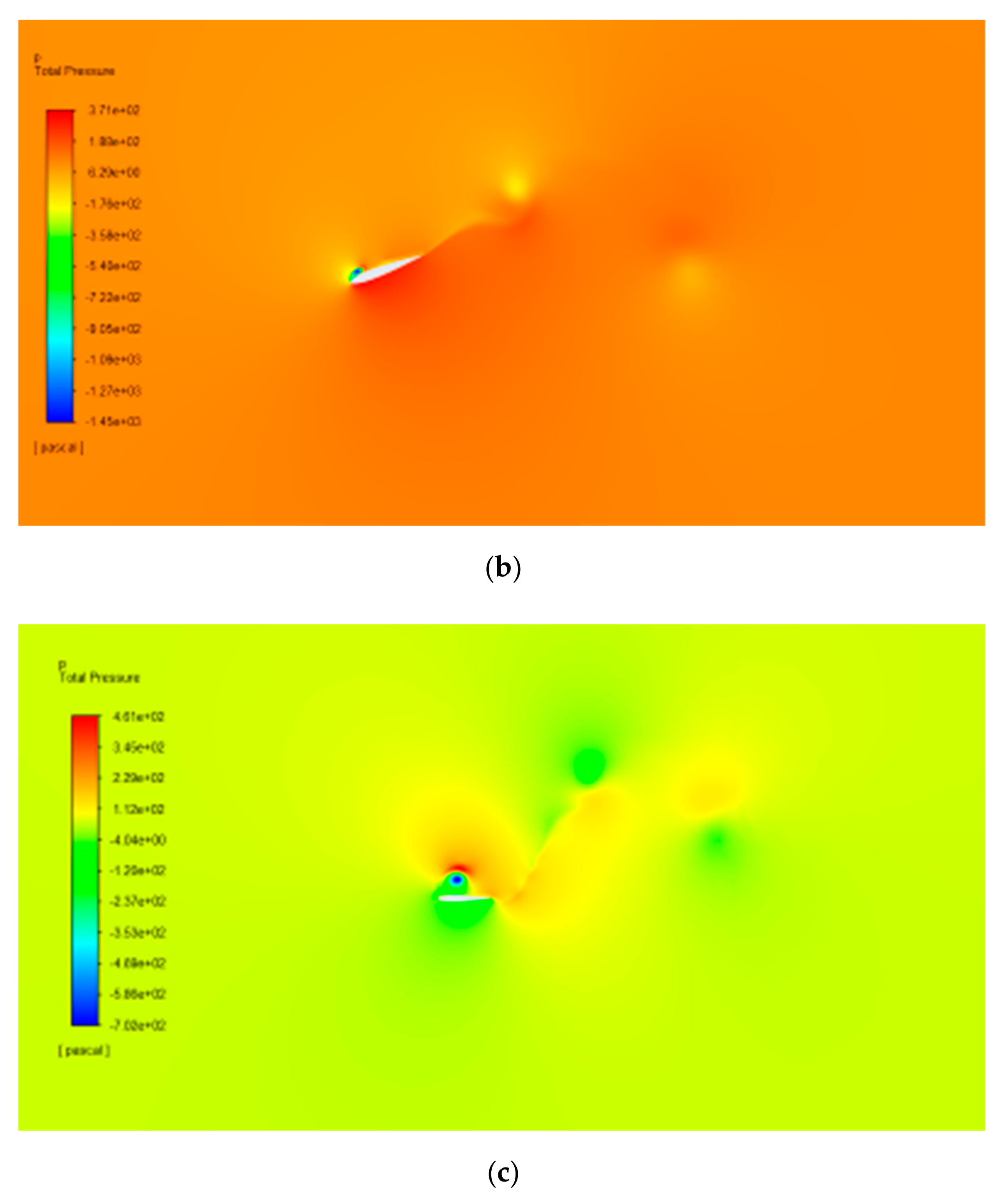
2.3. Mesh and Boundary Conditions

The numerical simulation is based on the Finite Volume Method (FVM) and is realized by FLUENT software, and the propulsion performance of the flapping hydrofoil is evaluated according to the calculated mechanical data. In this study, the computational domain is set from −20c to 60c in the horizontal direction, and from −20c to 20c in the vertical direction, and a mesh refinement area with a length of 12c and a height of 10c is set to ensure the calculation accuracy, as shown in Figure 3.

In the boundary condition settings, the upper and lower boundaries are set to simulate the infinite sea area and set to symmetry. The velocity inlet can be calculated according to the Reynolds number Re = 40,000 to obtain V = 0.4 m/s and set the outlet as the pressure outlet [21]. The upper and lower boundaries of the hydrofoil are set as no-slip walls. In order to capture the flow field changes at the edge of the flapping hydrofoil, unstructured grid technology was used to divide the flow field, and the rest of the watershed was also divided by sweep technology. The mesh details are shown in Figure 4.

2.4. Numerical Verification

For the convergence analysis of the calculation grid, three sets of grids are selected, and the grid quantities are 70,392, 188,110, and 268,185, respectively. The case where the maximum pitch angle is 15°, the vertical amplitude is c, and the phase difference between the surge motion and the heave motion is 75° are selected for calculation. The variation in thrust coefficient of different grid quantities in a single cycle is shown in Figure 5.

The difference in grid quantity among the three groups is mainly due to the difference in near-wall grid growth rate. Obviously, around 0.2 T, the calculated values of the 70,392 grids group have a large deviation from the other two groups. This indicates that when the thrust changes greatly, the requirement for the near-wall grid is higher and more grids are needed for the calculation. For the consideration of calculation accuracy and calculation speed, 188110 groups of grids were selected for calculation in this study.

In order to ensure the accuracy of the calculation results and avoid the time step affecting the calculation accuracy, according to YU, Esfahani [10,11], and others’ discussions, the calculation accuracy can be guaranteed when the time step ∆t = T/3000. In this study, in order to ensure the accuracy of numerical calculation, three groups of ∆t = T/3000, ∆t = T/3600, and ∆t = T/4000 were selected for trial calculation. The results are shown in Figure 6. It can be seen that the calculation results of the three groups of time steps almost overlap. In order to ensure the calculation accuracy, ∆t = T/3600 is selected as the time step.

The model adopts the k-ω (SST) two-equation turbulence model. Pressure-velocity coupling is performed using a pressure-based solver using the Pressure Implicit Splitting of Operator (PISO) algorithm. Second-order upwind is used to discretized governing equations on grid nodes. The flapping hydrofoil and its boundary layer move together, and the motion is compiled by a user-defined function according to Equations (1)–(3). Utilizing smoothing and remeshing techniques in dynamic mesh in flapping motion, in order to ensure the calculation accuracy, the maximum number of iterations of the moving grid is set to 100-times. Set the minimum dynamic grid size slightly smaller than the height of the first layer of the boundary layer grid. Control the calculation result accuracy and set the residual to 1e-05. Referring to Xiao Chen’s [12] calculation of the elliptical motion of the flapping hydrofoil, the above calculation method is used to calculate a set of numerical simulation results to complete the comparison and demonstration. Select the working condition of θ₀ = 23°, h₀ = 0.75c, φ = 60° for calculation. The calculation results are shown in

Table 1. Numerical Verification of Computational Methods.

	Ct
Xiao Chen	0.5662
This time	0.5642

. The difference between the two results is 0.353%. The small difference in the calculation may be due to a slight difference in the way the grid describes the hydrofoil or a difference in the size of the near-wall grid. However, a small calculation error is sufficient to prove the accuracy of the numerical simulation.

3. Results

All numerical calculation experiment groups were carried out according to the description of the motion trajectory above, and the motion trajectory was differentiated into the velocity equation according to Equations (1)–(3) and then compiled with UDF.

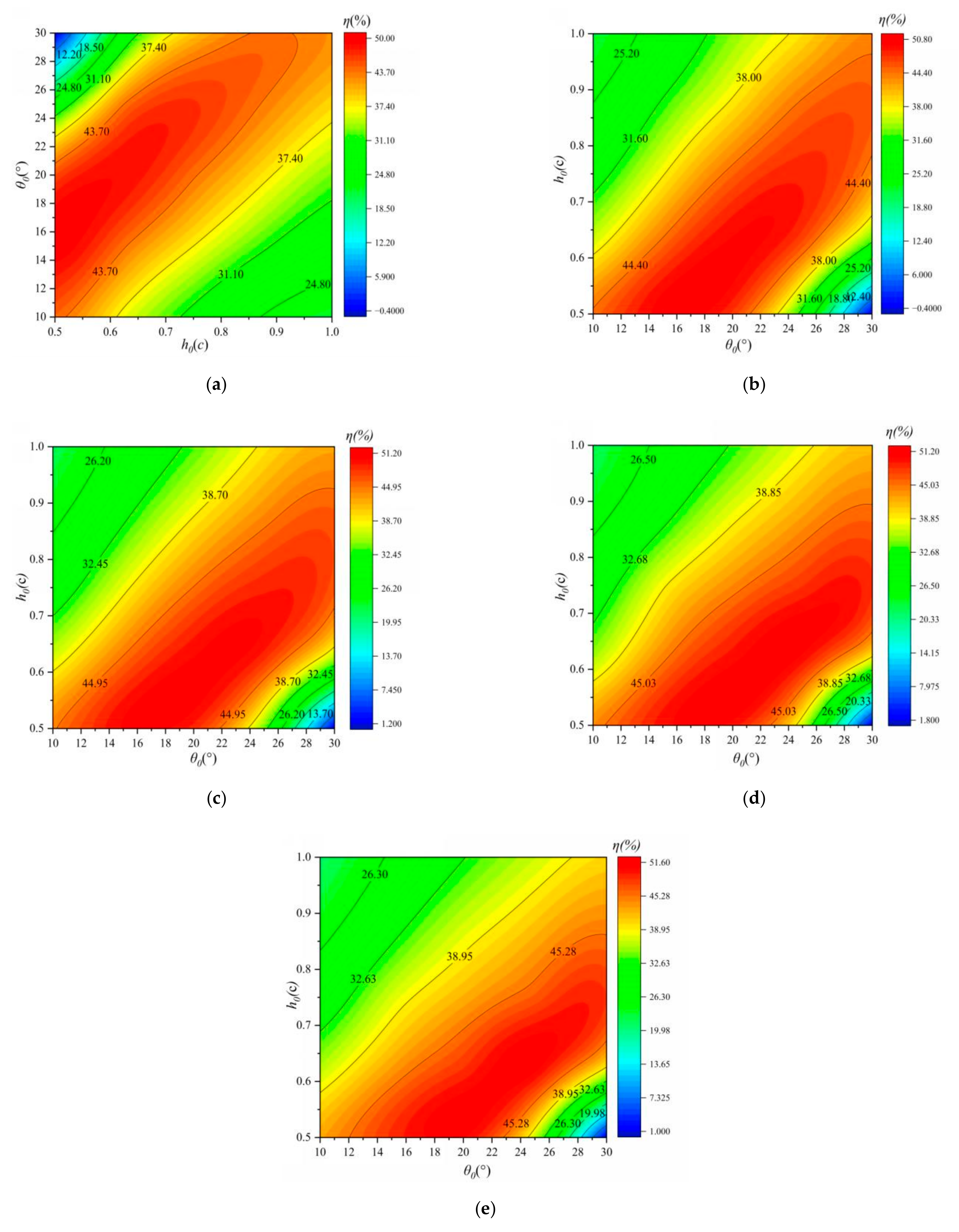
3.1. Influence of Heave Motion Amplitude on Propulsion Performance

As shown in Figure 7, the pressure contour changes at different times of θ₀ = 20°, h₀ = c, and φ = 120°. Figure 8 shows the variation in the average thrust coefficient with the heave amplitude under different phase differences that heave and surge motion and pitch amplitudes. The force generated by the flapping hydrofoil during the movement is generated by the interaction between the flapping hydrofoil and the flow field. The force is divided into two parts: part of the force is caused by the existence of the hydrofoil affecting the fluid flow, which is caused by the viscosity of the fluid and the roughness of the surface of the hydrofoil, so this part of the force is basically unchanged and does not change due to the movement of the flapping hydrofoil. The remaining part of the force is caused by the external force driving the hydrofoil movement, and the hydrofoil is caused by the reaction force of the fluid, and the size and action form of this part of the force is affected by the motion trajectory of the hydrofoil.

Obviously, the average thrust coefficient increases gradually with the increase in heave amplitude and exhibits certain linearity in Figure 8. According to Ding’s research, the thrust during flapping motion comes from the vortex generated by the flapping motion. In other words, the amplitude of the heave motion of the flapping hydrofoil is positively correlated with the vortex intensity [22,23].On the other hand, it can be found from Figure 8 that in the five sets of data with the pitch amplitude of 10°, 15°, 20°, 25°, and 30°, when the thrust is diminutive, other factors are certain, and the points under different phase differences between the heave and surge in Figure 8 almost overlap with the change in the phase difference and the difference in the average thrust coefficient between each phase difference gradually increases. This phenomenon shows that the vortex generated by the flapping motion is not only affected by the amplitude of the flapping heave motion, but also by the phase difference between the surge and the heave. Especially with a huge thrust, the impact on thrust is more obvious. The results show that the three motion parameters have an interactive effect on the thrust. (At different levels of heave amplitude, φ and θ₀ have different influences on the thrust coefficient.) Additionally, it can be found in Figure 8 that at different levels of h₀, there are differences in the influence of the change in φ on the thrust coefficient. At a larger heave amplitude, the influence of φ is greater, indicating that there is an interaction effect between φ and h₀ on the thrust coefficient.

In addition to the average thrust coefficient, another important factor in the propulsion performance of a flapping hydrofoil is the average propulsion efficiency. Figure 9 shows the distribution of the influence of heave amplitude on propulsion efficiency under different heave and surge phase differences and pitch amplitudes. Under different heave and surge phase differences, the high-efficiency regions are all distributed in oblique bands. Considering the change in heave amplitude for efficiency alone, the change in propulsion efficiency is also different under different pitch amplitudes. Taking φ = 60° as an example, when the pitch amplitude is in the range of 10° to 20°, the propulsion efficiency is inversely proportional to the heave amplitude. The situation changes when the pitch amplitude is in the range of 20~30°. The extreme value of propulsion efficiency appears in the range of heave amplitude variation. The above results show that when considering propulsion efficiency, the heave amplitude cannot be considered only.

3.2. Effect of Maximum Pitch Angle on Propulsion Performance

Analyzing the influence of pitch amplitude on the average thrust coefficient in Figure 10a–e, the curves of h₀ = 0.5c group all show the phenomenon that the average thrust coefficient decreases with the increase in pitch amplitude. The remaining four sets of curves h₀ = 0.625c, h₀ = 0.75c, h₀ = 0.875c, h₀ = c show that the average thrust coefficient increases first and then decreases with the increase in pitch amplitude. In other words, when the heave amplitude is at a low level, the increase in the pitch amplitude has a negative effect on the increase in the average thrust coefficient. When the heave amplitude is large, the elevation amplitude increases to a certain extent, which is beneficial to the improvement in the average thrust coefficient. The effect of pitch amplitude on the average thrust coefficient is affected by the level of heave amplitude. Different from the positive correlation between the heave amplitude and the average thrust coefficient, the pitch amplitude needs to determine the optimal parameters according to different heave amplitudes.

Furthermore, from the perspective of propulsion efficiency, as shown in Figure 11, h₀ = 0.5c, h₀ = 0.625c two sets of efficiency diagram analysis, the efficiency value increases first and then decreases with the rise in the pitch angle, indicating that the maximum value of the efficiency should appear between 18 and 24°. On the other hand, in the three groups of h₀ = 0.75c, h₀ = 0.875c, and h₀ = c, the efficiency value increases with the rise in pitch amplitude, and the high-efficiency area appears in the area of high pitch angle. Likewise, a larger pitch angle can be considered suitable for a higher heave amplitude. When analyzing the effect of pitch amplitude on propulsion efficiency, there is a dataset to consider: when h₀ = 0.5c, φ = 60°, θ₀ = 30° produces a negative thrust, and its propulsion efficiency is −0.35%. In contrast, when other factors remain unchanged, when θ₀ = 15°, the propulsion efficiency of flapping hydrofoil under this group of motion parameters can reach 49.77%, which is 50.12% higher than that when θ₀ = 30°. For the result analysis of pitch amplitude on propulsion efficiency, similar conclusions can be drawn from Yu’s research. At higher pitch amplitudes, the high-efficiency region appears at higher heave motion amplitudes [10]. For propulsion efficiency, the selection of pitch amplitude needs to be comprehensively judged according to other motion parameters to select the most suitable parameters. Similarly, this also shows that under different pitch amplitude levels, the influence of heave amplitude on thrust is different, reflecting that for thrust; there is also an interaction effect between heave amplitude and pitch amplitude.

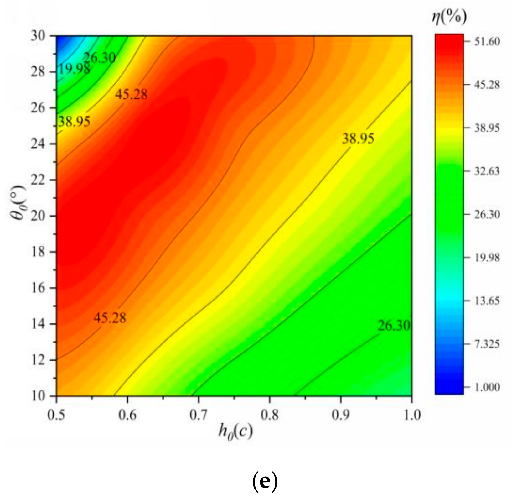
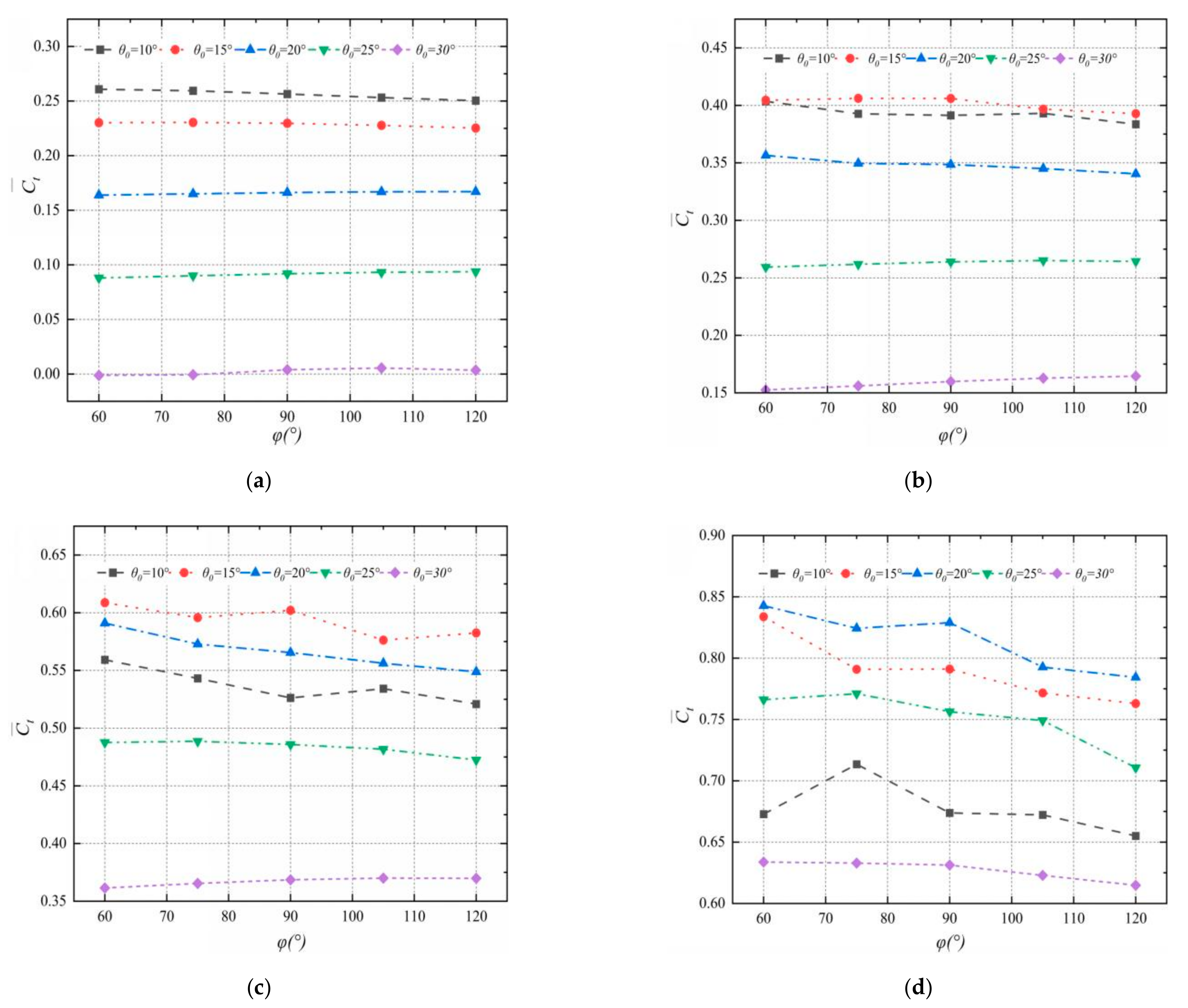
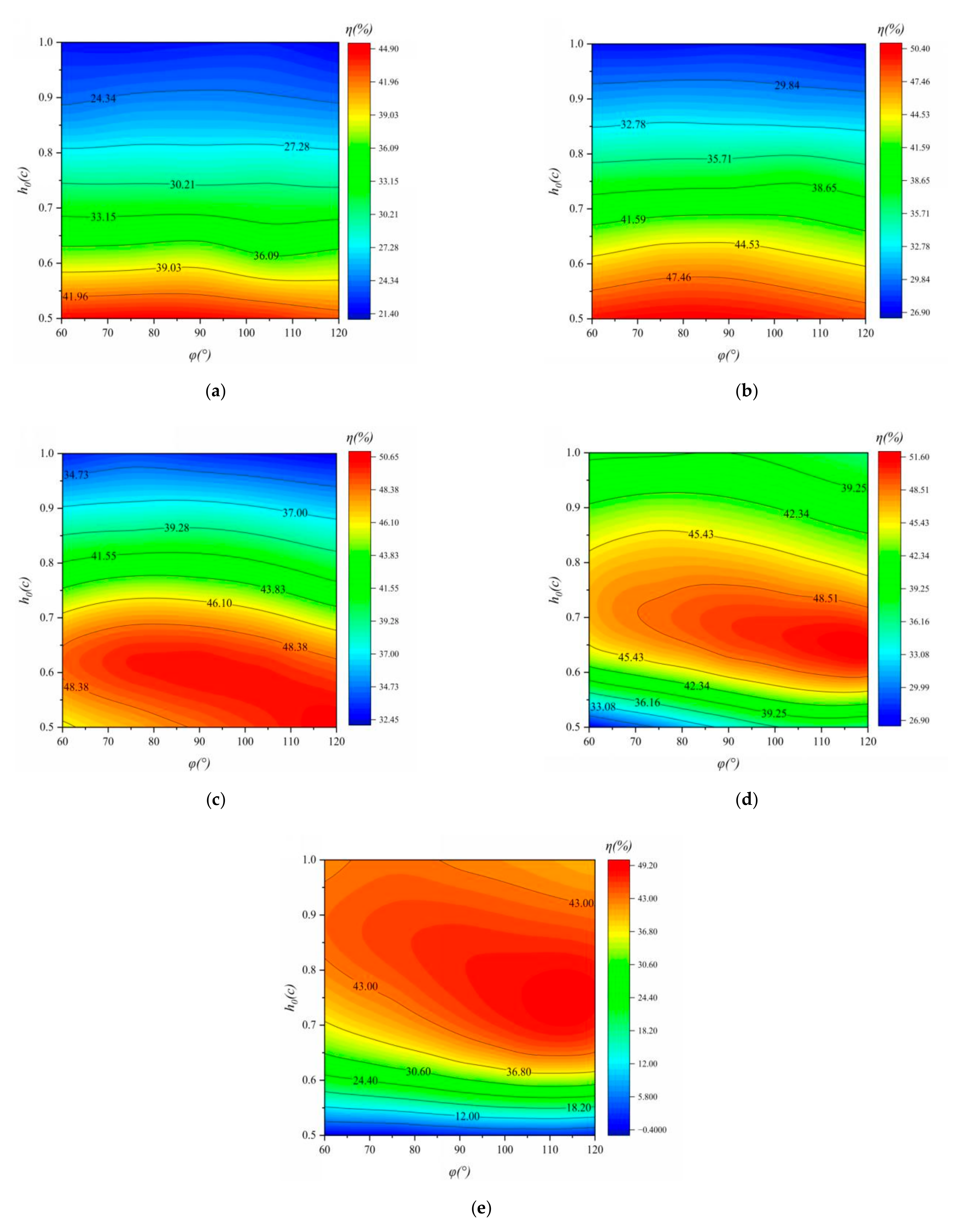
3.3. Influence of Heave Motion and Surge Motion Phase Difference on Propulsion Performance

Taking the average thrust coefficient as the observation index, it can be found from the figure that as the amplitude increases, the influence of the phase difference on the average thrust coefficient becomes more and more severe. The standard deviation of each experimental group calculated according to

Table 2. The standard deviation of thrust coefficient of different heave motion amplitudes and pitch amplitude curves.

	h0 (c)	0.5	0.625	0.75	0.875	1
θ0 (°)
10		0.00384	0.00639	0.01352	0.01931	0.04365
15		0.00192	0.00546	0.01206	0.02444	0.05122
20		0.00121	0.00532	0.01453	0.02231	0.03994
25		0.00212	0.00207	0.00589	0.02139	0.03729
30		0.00268	0.00438	0.00324	0.00727	0.02699

shows this phenomenon intuitively. (Table 2 shows the standard deviation values of each group of curves.)

For motion trajectories with large pitch and heave amplitude, the effect of φ is particularly important. As shown Figure 12. For example, when θ₀ = 20° and h₀ = c are affected by the phase difference between surge motion and heave motion, the difference between the maximum average thrust coefficient and the minimum average thrust coefficient is 0.0915, and the decrease is 8.21%. Therefore, it is necessary to consider the phase difference between heave and surge when designing the motion trajectory of a large thrust.

According to the previous research, the main reason for the thrust improvement in the elliptical motion trajectory compared with the two-degree-of-freedom trajectory is the mergeing of the leading-edge vortex and the trailing edge vortex during the flapping motion. If the phase difference between the surge and the heave is not properly controlled, and the directions of the leading and trailing edge vortex and the leading vortex are opposite, it may have an adverse effect.

For the two curves h₀ = 0.875c, θ₀ = 10°, h₀ = c, θ₀ = 15°, a bulge appears when φ = 75°, and the average thrust coefficient increases significantly compared to both sides. It can be judged that the optimum phase difference between these two motion trajectories is around 75°. However, when φ = 120°, each curve performs poorly, showing that when φ = 120°, it is not conducive to the fusion of the leading-edge vortex and the trailing edge vortex. In further research, focus should be placed in the range of 75–105°.

From the propulsion efficiency distribution diagram, as shown Figure 13, the phase difference between the heave and the surge affects the propulsion efficiency can be observed. Under the two sets of data of θ₀ = 10° and θ₀ = 15°, the efficiency contour does not change much with φ, indicating that the phase difference between the heave and the surge has little effect on the propulsion efficiency when the pitch amplitude is small. In the three groups of θ₀ = 20°, θ₀ = 25°, and θ₀ = 30°, it can be found that in the low-efficiency area, the efficiency contour is relatively flat, and the phase difference between the heave and the surge motion has little effect on the propulsion efficiency, but in the high-efficiency area, changes in φ significantly affect propulsion efficiency. The efficiency contour of the high-efficiency area has obvious fluctuations. This may be because, while in the high-efficiency region, the fusion of the leading edge and trailing edge vortices of the flapping wing have a greater impact on the thrust, and a suitable phase difference can improve the vortex intensity of the leading and trailing edge vortex mergers.

In previous research, adding a third degree of freedom in the horizontal direction to the traditional motion is beneficial to improving the propulsion performance. According to the paper of Chen et al. [12]. it can be seen that the propulsion performance will be better than the traditional two-degree-of-freedom motion in the case of x₀/h₀ = 0.5c, φ = 60~120°. In this study, h₀ = 0.5c and θ₀ = 10° were used as an example to calculate the results, which are shown in

Table 3. Comparison of propulsion performance between different phase differences and traditional two-degree-of-freedom motion under the premise of h₀ = 0.5c and θ₀ = 10°.

	Traditional Motion	φ = 60°	φ = 75°	φ = 90°	φ = 105°	φ = 120°
$\overline{C_t}$	0.2542	0.2608	0.2594	0.2565	0.2532	0.2505
Improvement	\	2.60%	2.05%	0.90%	−0.39%	−1.46%
$\overline{\eta }$	31.72%	44.55%	44.79%	44.61%	43.97%	42.80%
Improvement	\	12.83%	13.07%	12.89%	12.25%	11.08%

.

Under the premise of a certain phase difference in heave and surge, increasing the motion in the horizontal direction does improve the propulsion efficiency, as shown in Table 3. However, from the data of φ = 105° and φ = 120°, it can be found that the average thrust coefficient is slightly lower than that of the group without horizontal movement. Therefore, choosing the right phase difference helps to improve the propulsion performance of the flapping hydrofoil.

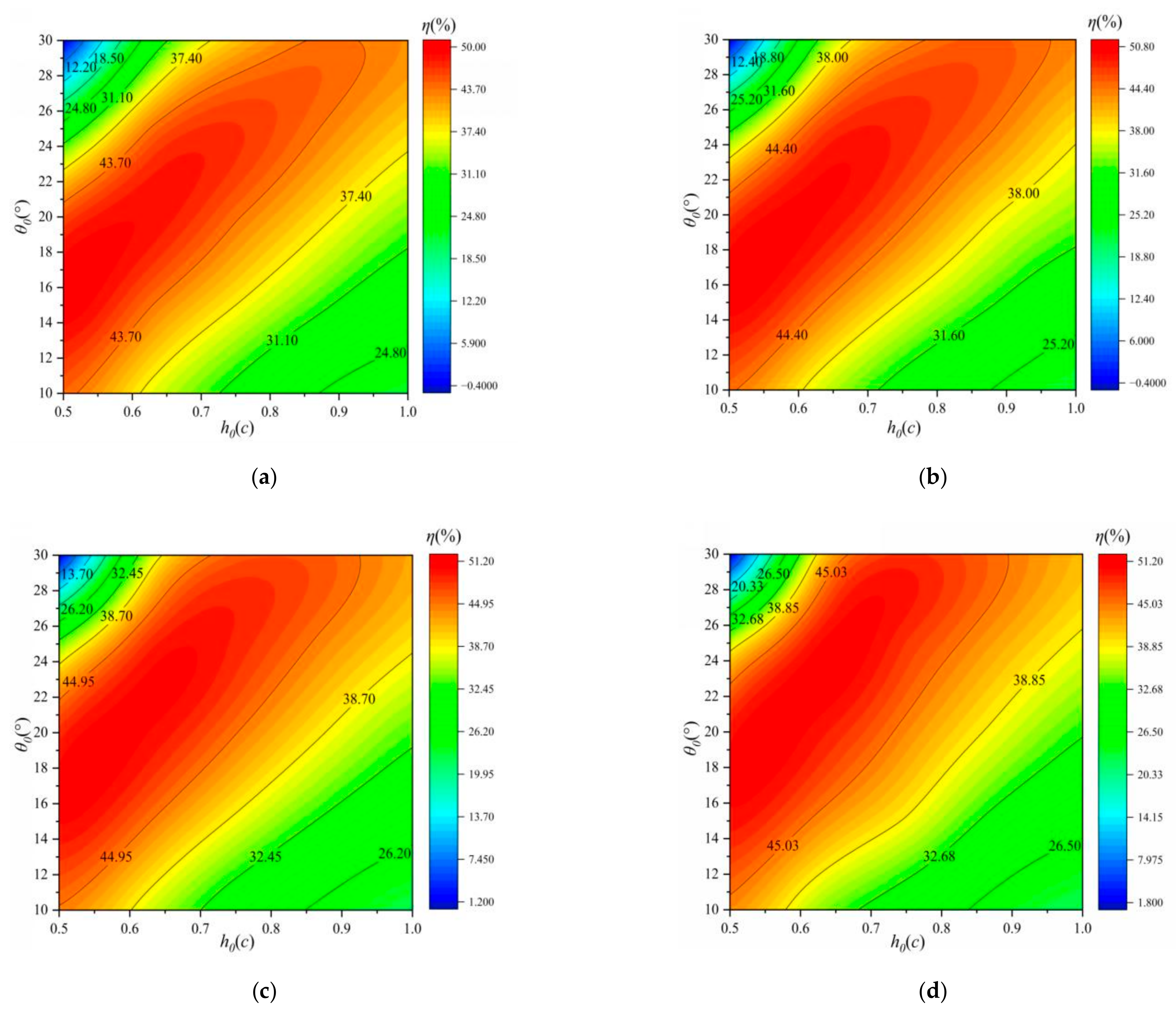
3.4. Optimal Matching Results

Based on the above research, it is shown that for the study of the hydrofoil trajectory, three motion parameters have interactive effects on thrust; the three factors h₀, θ₀, and φ should be considered together. Involving the optimization problem of the three factors, in order to obtain the optimal propulsion efficiency under a certain thrust, which involves multi-factor optimal analysis, this paper uses the BP (back propagation) neural network in deep learning to fit the functional relationship between the motion parameters and the thrust coefficient and propulsion efficiency and obtain the optimal choice.

The structure of the BP neural network is shown in the Figure 14, which has three or more layers of the neural network, including an input layer, hidden layer, and output layer. The upper and lower layers are fully connected, and there is no connection between neurons in each layer. After learning the sample is provided to the network, the activation value of the neuron goes from the input layer through the hidden layer to the output layer and then proceeds in the direction of reducing the error between the expected output and the actual output [24,25].

The pitch amplitude, the heave amplitude, the phase difference between the heave and the surge, and the average thrust coefficient are normalized, and the functions of the average thrust coefficient and the three motion parameters are fitted. A fitting function is established between the three motion parameters and the average propulsion efficiency, and the motion parameter group that meets the thrust conditions is input into the fitting function to obtain its motion efficiency, and the motion parameter group with the maximum propulsion efficiency is selected from it.

The calculated 100 sets of numerical simulation data were input as training samples for fitting, and the remaining 25 sets of data were used as validation samples for the fitted curve. The comparison between the fitted curve and the actual data curve is shown in Figure 15.

Selecting h₀ = 0.5c, θ₀ = 10°, φ = 120° group for optimal matching, C_t = 0.2504, ƞ = 42.8%, so that the output thrust coefficient is constant at 0.2504. The predicted motion parameter groups are compared and verified by Computational Fluid Dynamic (CFD) technology, and the obtained data are shown in

Table 4. Optimized propulsion performance and traditional comparison results and errors.

	Initial Motion Parameters (h0 = 0.5c, θ0 = 10°, φ = 120°)	Predicted Motion Parameters (h0 = 0.5095c, θ0 = 22.476°, φ = 96°)	CFD Validation of Predicted Motion Parameters (h0 = 0.5095c, θ0 = 22.476°, φ = 96°)
$\overline{C_t}$	0.2504	0.2504	0.2559
$\overline{\eta }$	42.80%	50.28%	50.53%
Improvement	\	\	7.73%

.

According to the data in Table 4, it can be found that the error of the thrust coefficient obtained by using the BP neural network fitting function and CFD calculation is 2.20%, which indicates that the function is well fitted. A functional relationship between motion parameters and propulsion performance is established through a certain amount of data. Using this method improves the propulsion efficiency by 7.73% compared with the method of directly specifying the motion parameter value. It shows that in the actual use of underwater vehicles, determining a target thrust, selecting motion trajectory parameters that are easy to control and changing, and a function fitted according to a certain amount of data points can effectively guide people to select the combination of motion parameters with the best propulsion performance. Figure 16 shows the one-cycle thrust coefficient change in the traditional two-dimensional motion and the motion trajectory before and after optimal matching. In the time period from 0 to 0.3 T, the thrust coefficient does not change significantly before and after optimal matching. However, in the range of 0.4 T to 0.7 T, the thrust coefficient is significantly improved, which may also be the main reason for the improvement of propulsion efficiency. Moreover, in the time period from 0.2 T to 0.7 T, the pulsation amplitude of the thrust coefficient is significantly improved compared with that before the optimal matching. The reason for the increase in the pulsation amplitude may be that the heave and pitch amplitudes of the motion after optimal matching have increased compared to the motion trajectory without optimal matching. Otherwise, the increase in thrust coefficient pulsation amplitude may affect the increase in propulsion shafting vibration. This may have a detrimental effect on noise reduction but has a positive effect on the improvement in propulsion efficiency.

4. Discussion

In this study, the effects of pitch amplitude, heave amplitude, surge and heave phase difference on the propulsion performance of flapping hydrofoil are considered, and three factors were comprehensively analyzed. The BP neural network is used to fit the motion parameters and the propulsion performance parameters to find the optimal motion trajectory under a certain thrust. The conclusions can be summarized as follows:

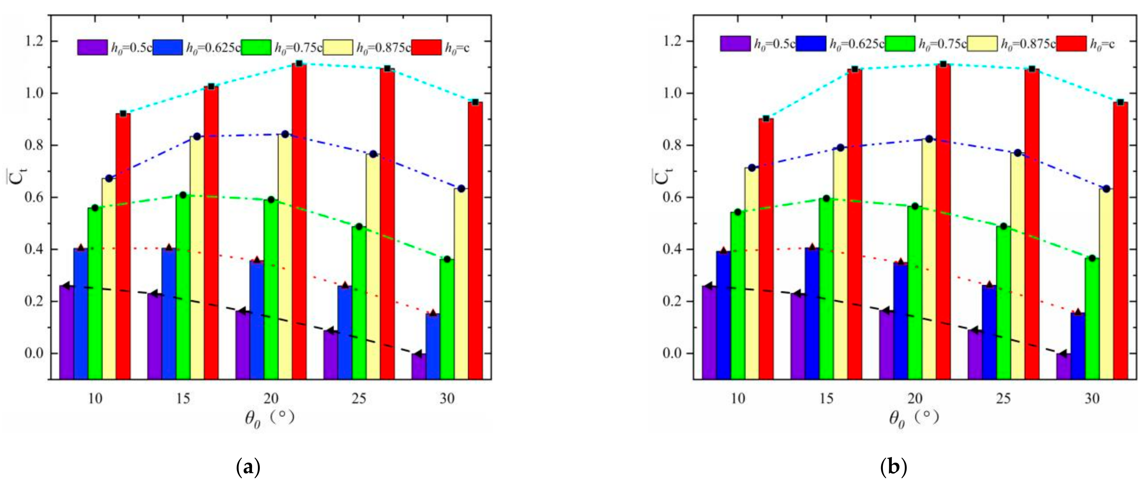
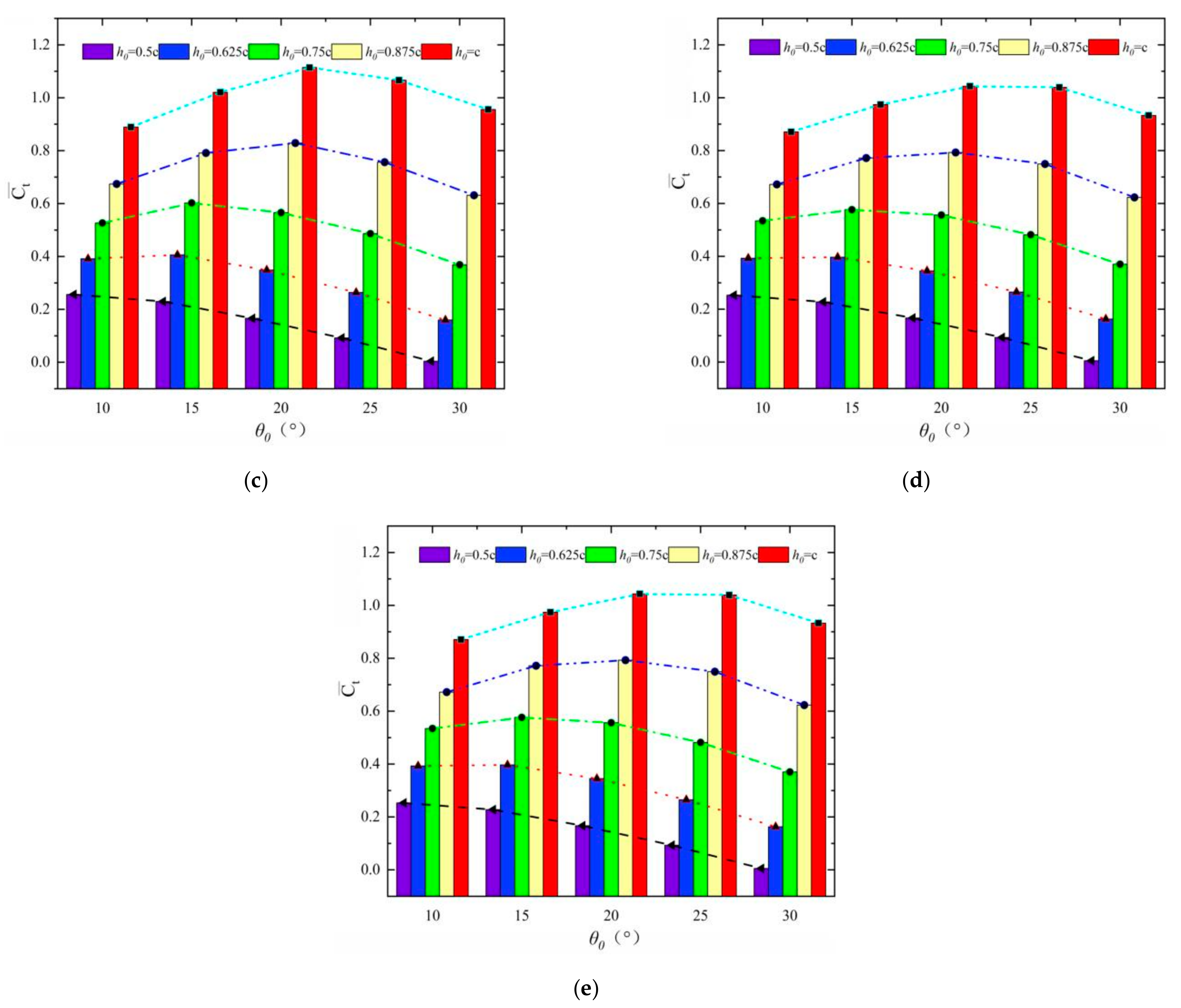
• The heave amplitude is positively correlated with the thrust coefficient. In addition, h₀, θ₀ and φ have interactive effects on the thrust coefficient of flapping hydrofoil, when the heave amplitude is at a higher level, the pitch amplitude, surge and heave phase difference have a greater impact on the thrust coefficient, and the interaction effect is more obvious.
• The difference between surge and heave had a greater impact on the high propulsive efficiency area, and the change in efficiency contour was more obvious than that of the low-efficiency area.
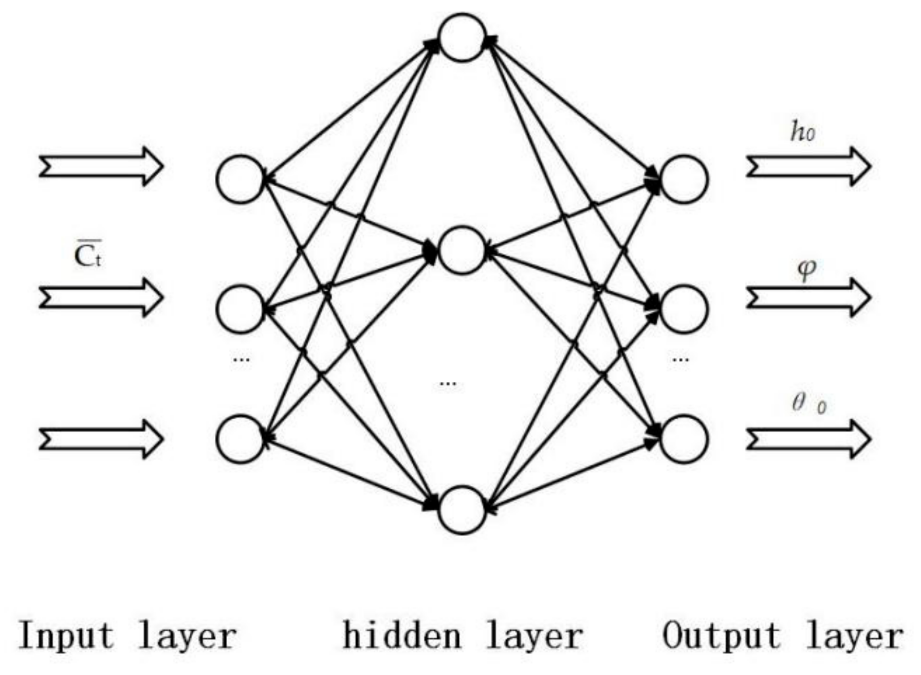
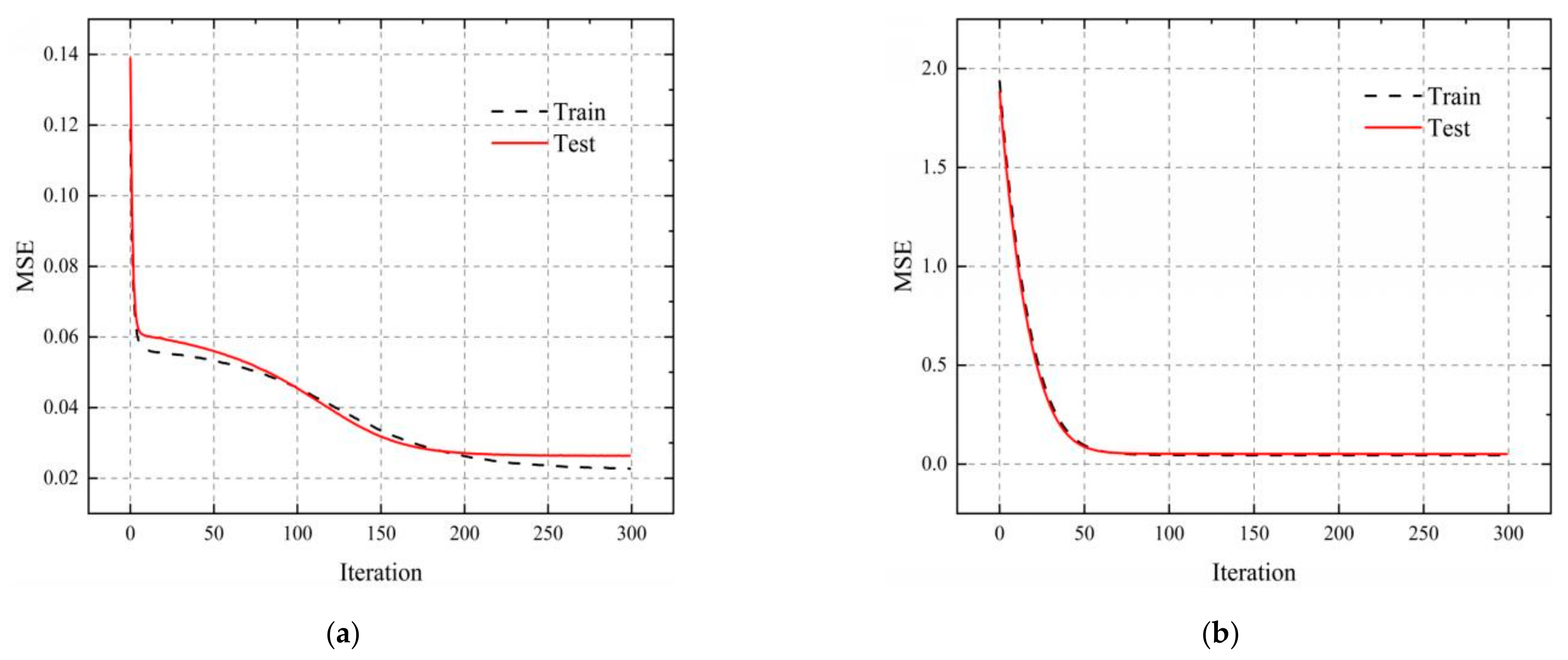
• Based on elliptical motion trajectory, the BP neural network was used to establish the fitting function of motion parameters and propulsion performance, and the motion parameter combination with the highest propulsion efficiency under certain thrust was obtained. When K_t = 0.2504, the propulsion efficiency could be improved by 7.73%.
• A new method to improve the propulsion performance of flapping hydrofoil is presented. By establishing the fitting function between the motion parameters and the propulsion performance, the optimal trajectory under certain thrust can be quickly found within the set motion parameters. This method can improve the propulsion performance of flapping hydrofoil and predict the optimal trajectory parameters under certain thrust.
• In this study, the propulsion performance of flapping hydrofoils is optimized based on elliptic trajectories, which can be applied to other trajectories in the future. The optimal motion models obtained under different motion trajectories are compared, and the flapping motion model with better propulsion performance can be obtained.

References

1. Yamaguchi, H.; Bose, N. Oscillating foils for marine propulsion. In Proceedings of the Fourth International Offshore and Polar Engineering Conference (One Petro), Osaka, Japan, 10–15 April 1994. [Google Scholar]
2. Ma, P.; Liu, G.; Wang, Y.; Zhang, Y.; Xie, Y. Numerical study on the hydrodynamic performance of a semi-passive oscillating hydrofoil. Ocean Eng. 2021, 223, 108649. [Google Scholar] [CrossRef]
3. Zhou, D.; Cao, Y.; Sun, X. Numerical study on energy-extraction performance of a flapping hydrofoil with a trailing-edge flap. Ocean Eng. 2021, 224, 108756. [Google Scholar] [CrossRef]
4. Triantafyllou, M.S.; Techet, A.H.; Hover, F.S. Review of Experimental Work in Biomimetic Foils. IEEE J. Ocean. Eng. 2004, 29, 585–594. [Google Scholar] [CrossRef] [Green Version]
5. Techet, A.H. Propulsive performance of biologically inspired flapping foils at high Reynolds numbers. J. Exp. Biol. 2008, 211, 274–279. [Google Scholar] [CrossRef] [PubMed] [Green Version]
6. Ashraf, M.A.; Young, J.; Lai, J.C.S. Reynolds number, thickness and camber effects on flapping airfoil propulsion. J. Fluids Struct. 2011, 27, 145–160. [Google Scholar] [CrossRef]
7. Read, D.A.; Hover, F.S.; Triantafyllou, M.S. Forces on oscillating foils for propulsion and maneuvering. J. Fluids Struct. 2003, 17, 163–183. [Google Scholar] [CrossRef]
8. Hover, F.S.; Haugsdal, Ø.; Triantafyllou, M.S. Effect of angle of attack profiles in flapping foil propulsion. J. Fluids Struct. 2004, 19, 37–47. [Google Scholar] [CrossRef] [Green Version]
9. Triantafyllou, G.S.; Triantafyllou, M.S.; Grosenbaugh, M.A. Optimal Thrust Development in Oscillating Foils with Application to Fish Propulsion. J. Fluids Struct. 1993, 7, 205–224. [Google Scholar] [CrossRef]
10. Yu, D.; Sun, X.; Bian, X.; Huang, D.; Zheng, Z. Numerical study of the effect of motion parameters on propulsive efficiency for an oscillating airfoil. J. Fluids Struct. 2017, 68, 245–263. [Google Scholar] [CrossRef]
11. Esfahani, J.A.; Barati, E.; Karbasian, H.R. Fluid structures of flapping airfoil with elliptical motion trajectory. Comput. Fluids 2015, 108, 142–155. [Google Scholar] [CrossRef]
12. Chen, X.; Huang, Q.; Pan, G.; Li, F. Numerical Investigation of Elliptical Motion on Propulsion Performance of a Flapping Hydrofoil. In Proceedings of the 2018 OCEANS—MTS/IEEE Kobe Techno-Ocean (OTO), Kobe, Japan, 28–31 May 2018. [Google Scholar]
13. Yang, S.; Liu, C.; Wu, J. Effect of motion trajectory on the aerodynamic performance of a flapping airfoil. J. Fluids Struct. 2017, 75, 213–232. [Google Scholar] [CrossRef]
14. Zhang, Y.; Yang, F.; Wang, D.; Jiang, X. Numerical investigation of a new three-degree-of-freedom motion trajectory on propulsion performance of flapping foils for UUVs. Ocean Eng. 2021, 224, 108763. [Google Scholar] [CrossRef]
15. Yue, W. Optimal design for flapping airfoil motion parameters. J. Beijing Univ. Aeronaut. Astronaut. 2021, 1–15. [Google Scholar]
16. Xingjian, L.; Jie, W.; Tongwei, Z. Self-organizing behavior during propulsion of flapping wing swarms. In Proceedings of the 11th National Academic Conference on Fluid Mechanics, Shenzhen, Guangdong, China, 3–7 December 2020; p. 700. [Google Scholar]
17. Isogai, K.; Shinmoto, Y.; Watanabe, Y. Effects of dynamic stall on propulsive efficiency and thrust of flapping airfoil. Aiaa J. 1999, 37, 1145–1151. [Google Scholar] [CrossRef]
18. Xianqi, Z.; Xiangcheng, S.; Xian, W. High-performance numerical study on the effect of angle of attack on the aerodynamic performance of flapping wing motion. Acta Aerodyn. 2021, 1–11. [Google Scholar]
19. Young, J. Numerical Simulation of the Unsteady Aerodynamics of Flapping Airfoils. Ph.D. Thesis, University of New South Wales, Sydney, Australia, 2005. [Google Scholar]
20. Anderson, J.M.; Streitlien, K.; Barrett, D.S.; Triantafyllou, M.S. Oscillating foils of high propulsive efficiency. J. Fluid Mech. 1998, 360, 41–72. [Google Scholar] [CrossRef] [Green Version]
21. Xiao, Q.; Zhu, Q. A review on flow energy harvesters based on flapping foils. J. Fluids Struct. 2014, 46, 174–191. [Google Scholar] [CrossRef]
22. Hao, D. Research on propulsion characteristics and motion performance of bionic flapping-wing underwater vehicle. Ph.D. Thesis, Northwestern Polytechnical University, Xi’an, China, 2015. [Google Scholar]
23. Xiaobai, L. Research on flexible hydrofoil propulsion technology imitating sea turtle. Ph.D. Thesis, Harbin Engineering University, Harbin, China, 2012. [Google Scholar]
24. Dehu, Q.; Jichang, K. Design of BP Neural Network. Comput. Eng. Des. 1998, 2, 47–49. [Google Scholar]
25. Zhibo, Z. Based on BP artificial neural network and genetic algorithm Optimum Design of Ship Propellers. J. Ship Mech. 2010, 20–27. [Google Scholar]
Figure 1. Three movement modes of flapping hydrofoil.
Jmse 10 00853 g001
Figure 2. Elliptical motion trajectories under different phase differences.
Jmse 10 00853 g002
Figure 3. Calculation area.
Jmse 10 00853 g003
Figure 4. Mesh details.
Jmse 10 00853 g004
Figure 5. (a) variation of thrust coefficient in one cycle of different grids, (b) enlarged part of figure (a).
Jmse 10 00853 g005
Figure 6. θ0 = 10°, h0 = 0.5c thrust variation diagram at different time steps.
Jmse 10 00853 g006
Figure 7. Pressure contour at different times (The left side is the pressure contour; the right side is the velocity contour) (a) t = 0.25 T (b) t = 0.5 T (c) t = 0.75 T.
Jmse 10 00853 g007aJmse 10 00853 g007b
Figure 8. Variation of average thrust coefficient with amplitude under different pitch amplitudes and phase differences (a) θ0 = 10° (b) θ0 = 15° (c)θ0 = 20° (d) θ0 = 25° (e) θ0 = 30°.
Jmse 10 00853 g008
Figure 9. Variation of average propulsion efficiency with heave motion amplitude under different phase differences and pitch amplitudes (a) φ = 60° (b) φ = 75° (c) φ = 90° (d) φ = 105° (e) φ = 120°.
Jmse 10 00853 g009aJmse 10 00853 g009b
Figure 10. Variation of average thrust coefficient with pitch amplitude under different phase differences and heave motion amplitudes (a) φ = 60° (b) φ = 75° (c) φ = 90° (d) φ = 105° (e) φ = 120°.
Jmse 10 00853 g010aJmse 10 00853 g010b
Figure 11. Variation of average propulsion efficiency with pitch amplitude under different heave motion amplitudes and phase differences (a) φ = 60° (b) φ = 75° (c) φ = 90° (d) φ = 105° (e) φ = 120°.
Jmse 10 00853 g011
Figure 12. Variation of average thrust coefficient with phase difference under different phase differences and pitch amplitude (a) h0 = 0.5c (b) h0 = 0.625c (c) h0 = 0.75c (d) h0 = 0.875c (e) h0 = c.
Jmse 10 00853 g012aJmse 10 00853 g012b
Figure 13. Variation of propulsion efficiency with the phase difference between heave and surge under different pitch amplitudes (a) θ0 = 10° (b) θ0 = 15° (c) θ0 = 20° (d) θ0 = 25°(e) θ0 = 30°.
Jmse 10 00853 g013
Figure 14. Schematic diagram of the BP neural network structure.
Jmse 10 00853 g014
Figure 15. (a) Mean square error iterative curve of motion parameter and average thrust coefficient fitting function (b) Mean square error iterative curve of the fitting function between motion parameters and average propulsion efficiency.
Jmse 10 00853 g015
Figure 16. Variation of thrust coefficient in one cycle before and after optimal matching.
Jmse 10 00853 g016