
Dynamic Analysis of Bottom Subsidence of Benthic Lander


Abstract
:1. Introduction
2. Methods
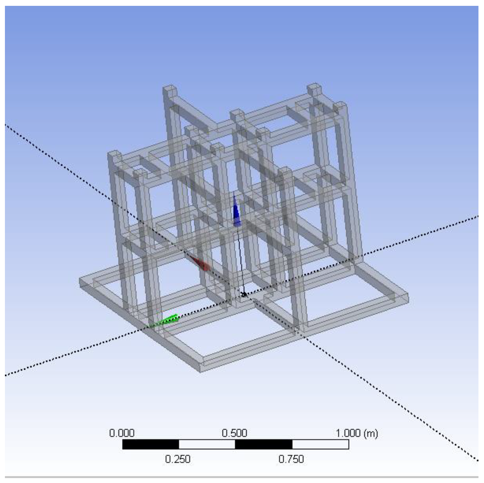
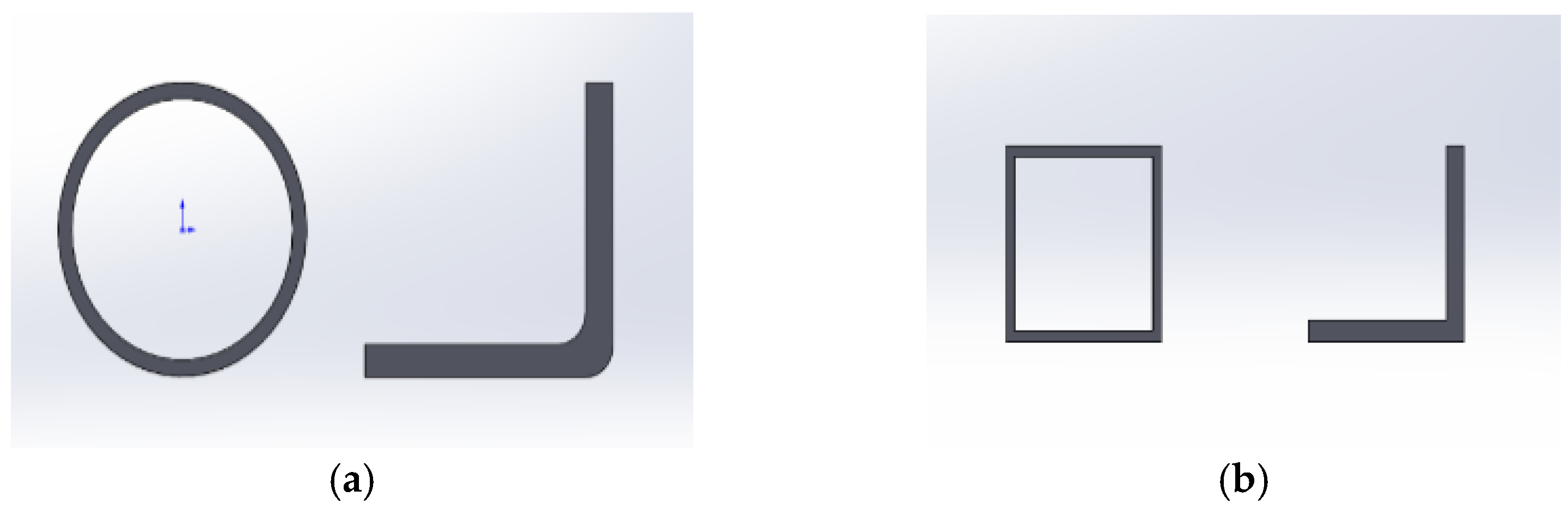
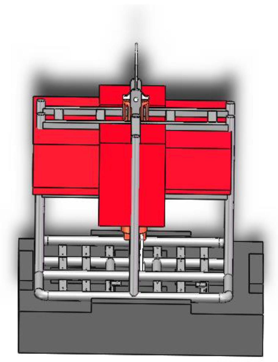
2.1. Statics Model of the Frame
2.2. Kinetic Model of the Benthic Lander
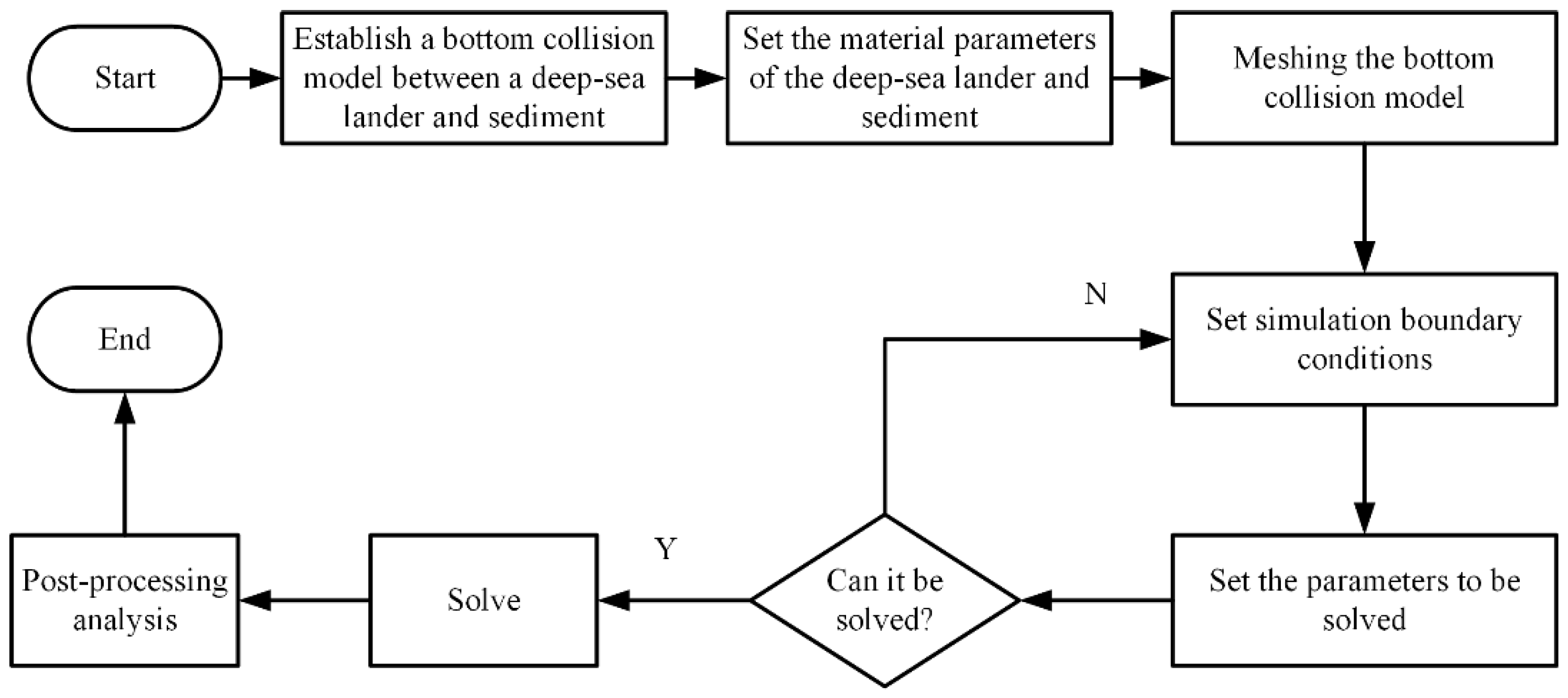
2.3. Finite Element Analysis with ANSYS
- Initial speed
- Simulation duration
- Constraints
3. Results and Discussion
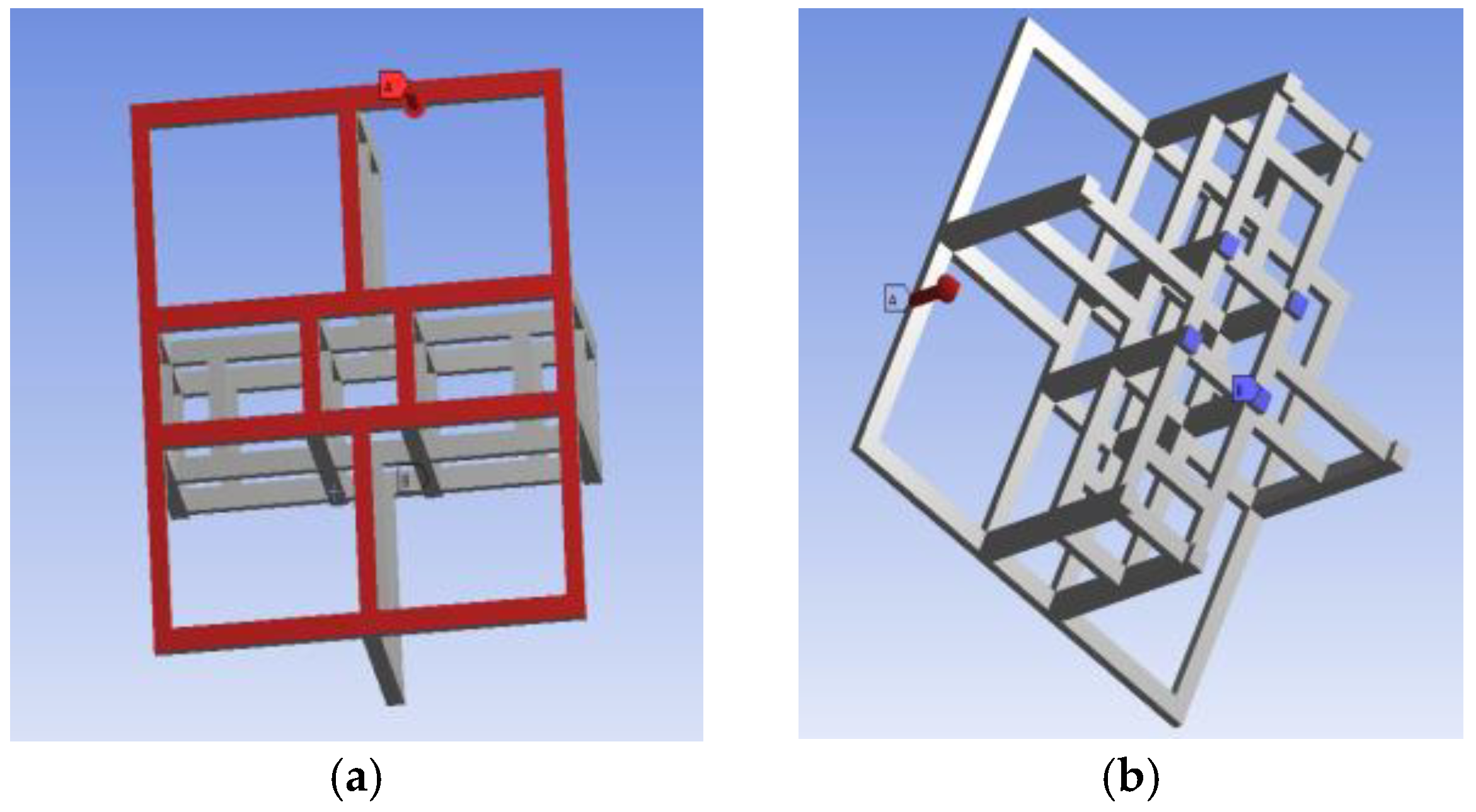
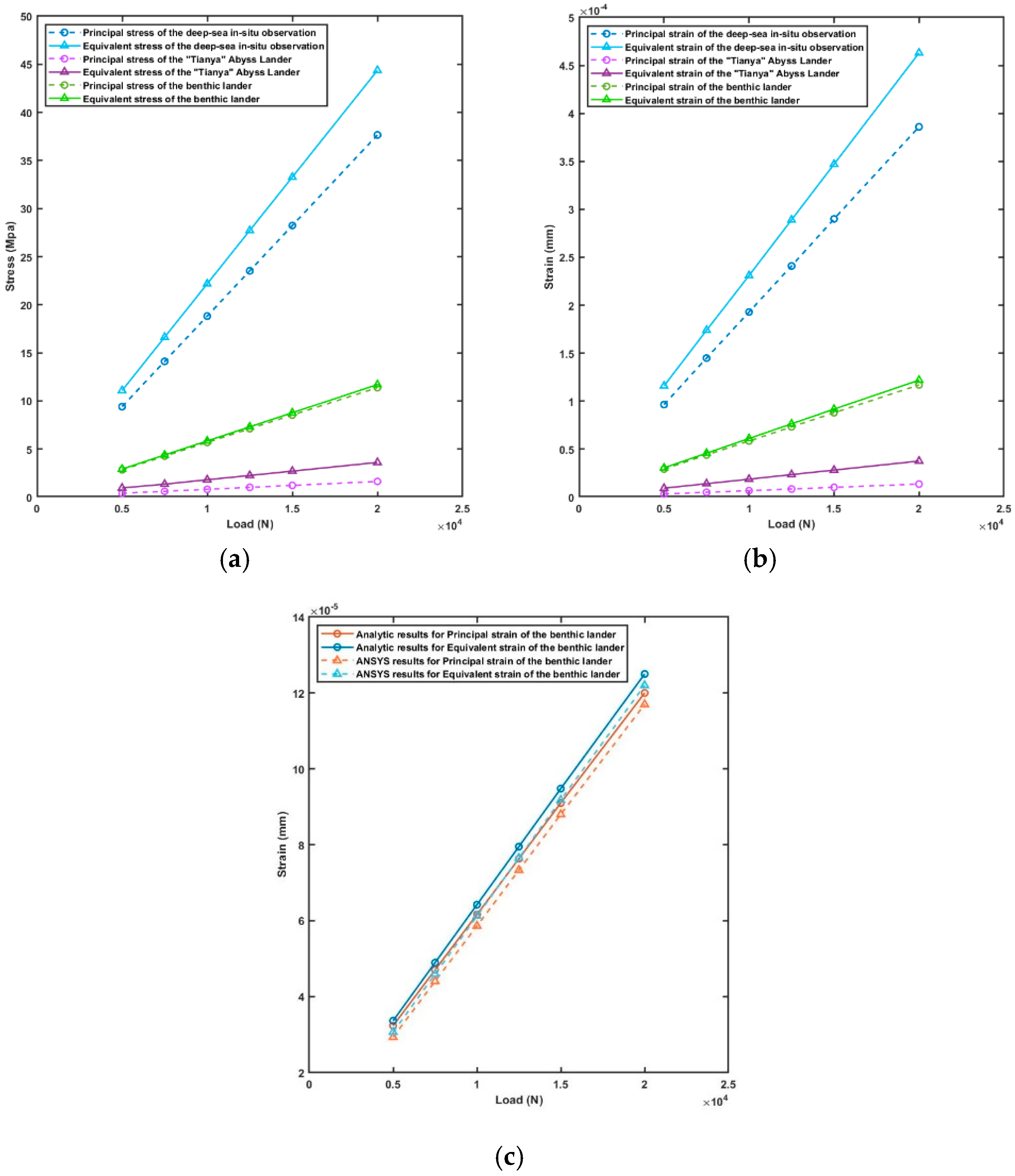
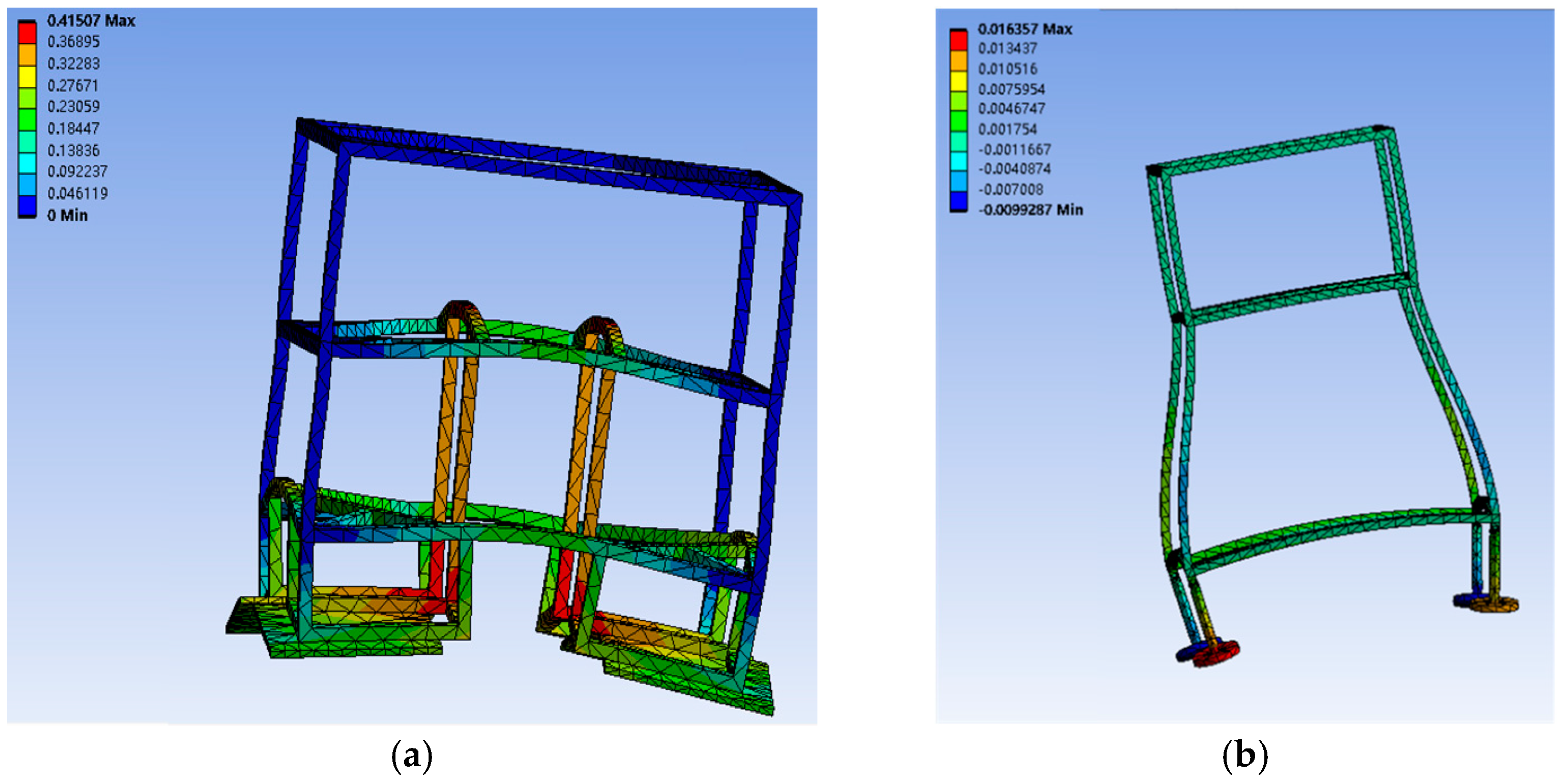
3.1. Analysis of Statics Simulation Results of Frames
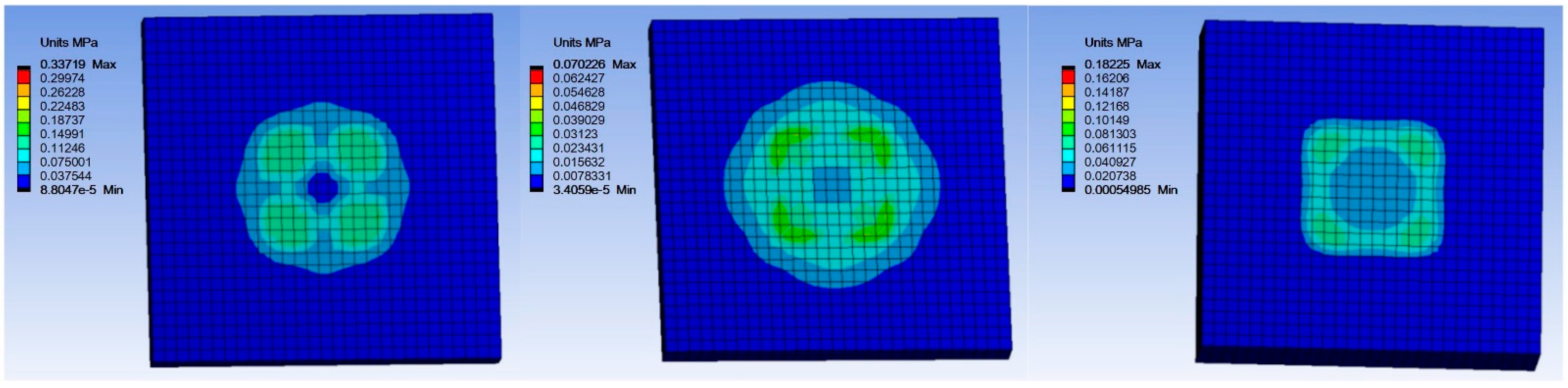
- When the frame of the benthic lander designed in this paper is subjected to force, the pillars shrink and deform inward, and the deformation in the middle of the frame is obviously smaller than that in the surrounding area.
- The support frame of the open frame lander can be designed at a certain angle to effectively reduce the deformation of the upper frame.
- Symmetrical addition of support columns and reinforcement bars inside the open frame can reduce deformation to a limited extent.
3.2. Analysis of Dynamic Simulation Results of Bottom Subsidence Process of Frames
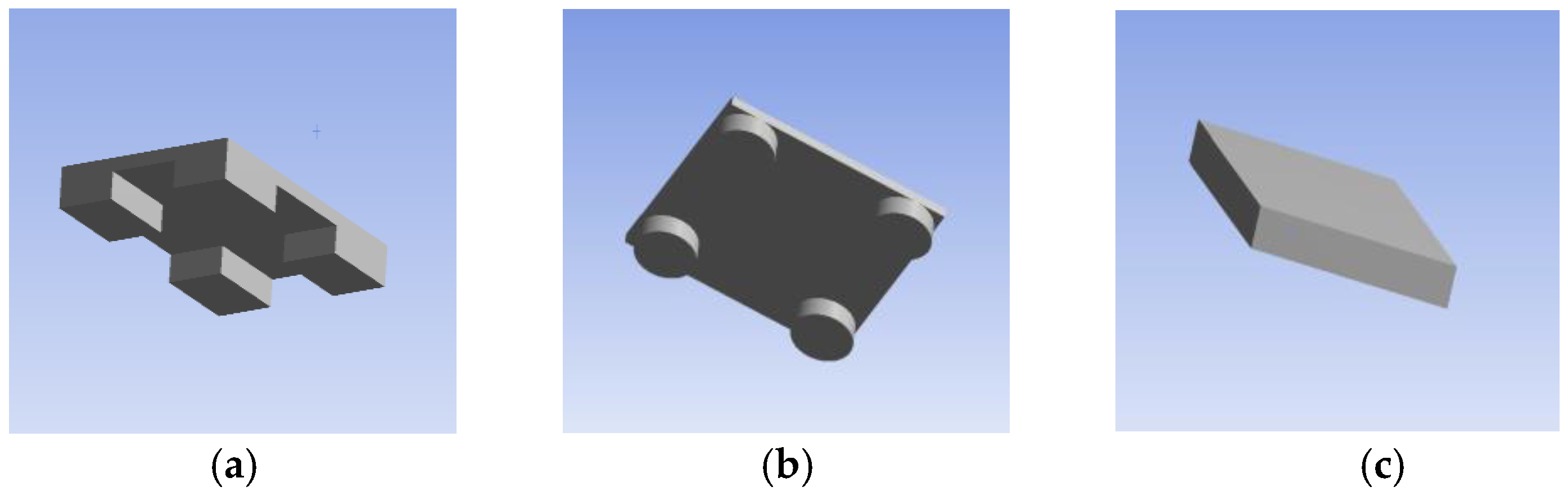
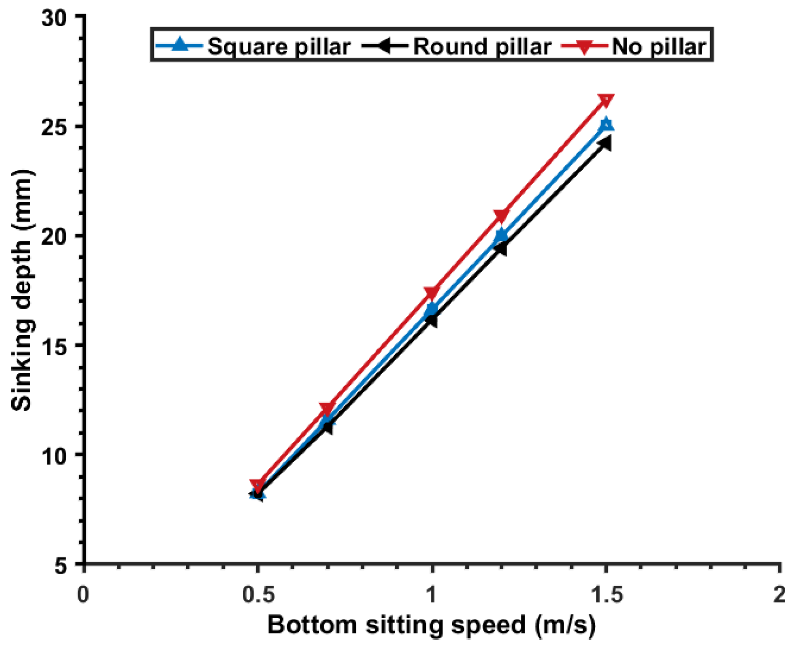
3.2.1. Bottom Shapes of Frames
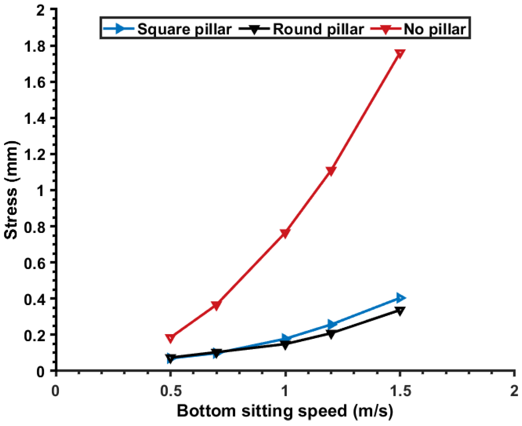
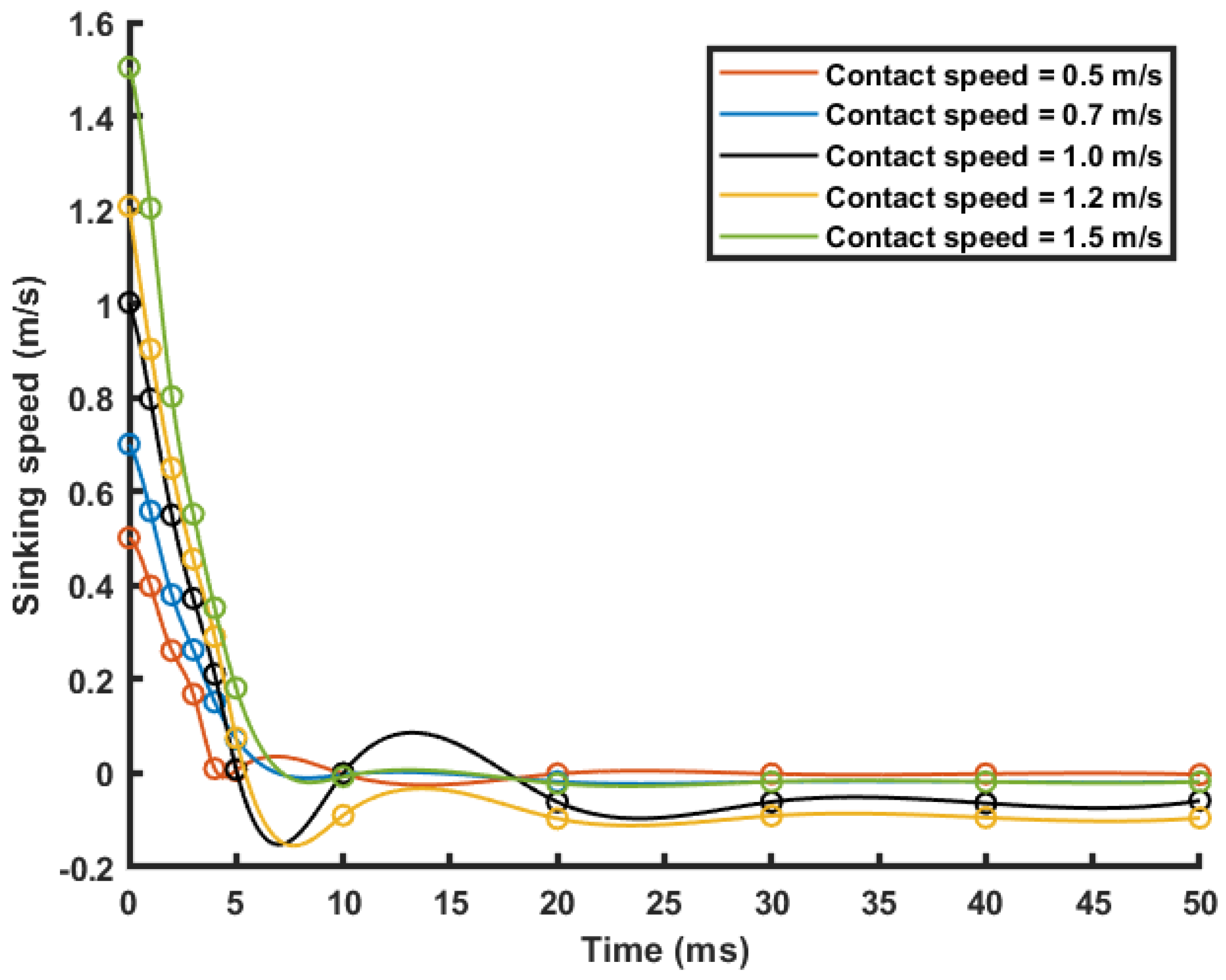
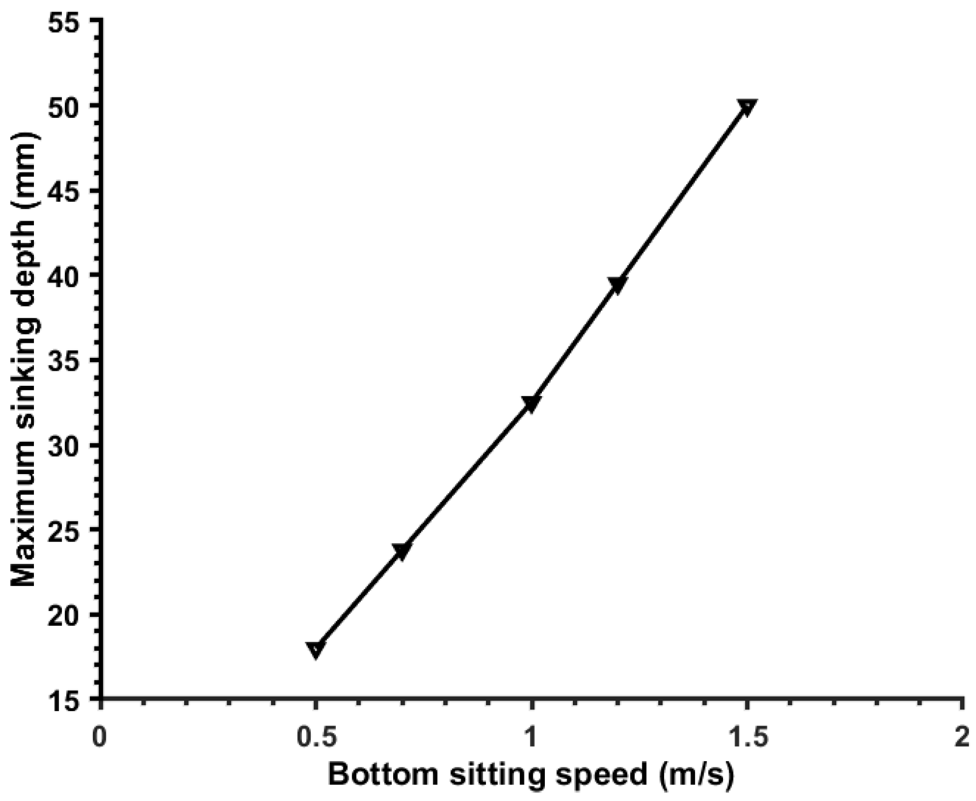
3.2.2. Analysis of the Collision Process between the Frame and the Sediment
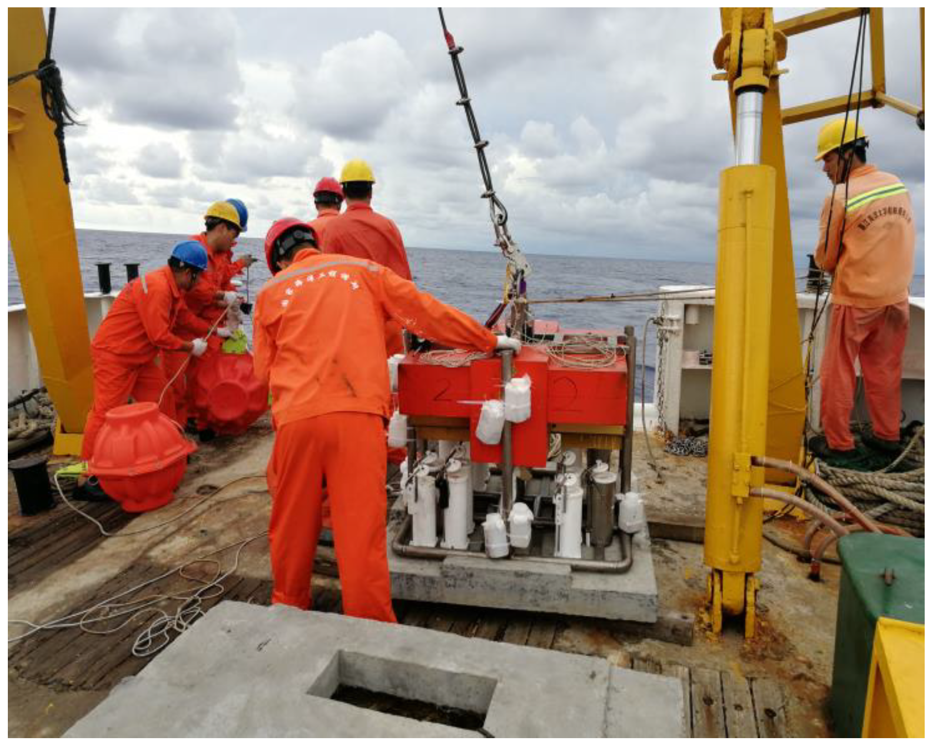
4. Experiments
4.1. Sea Trial Process
4.2. Sea Trial Results and Analysis
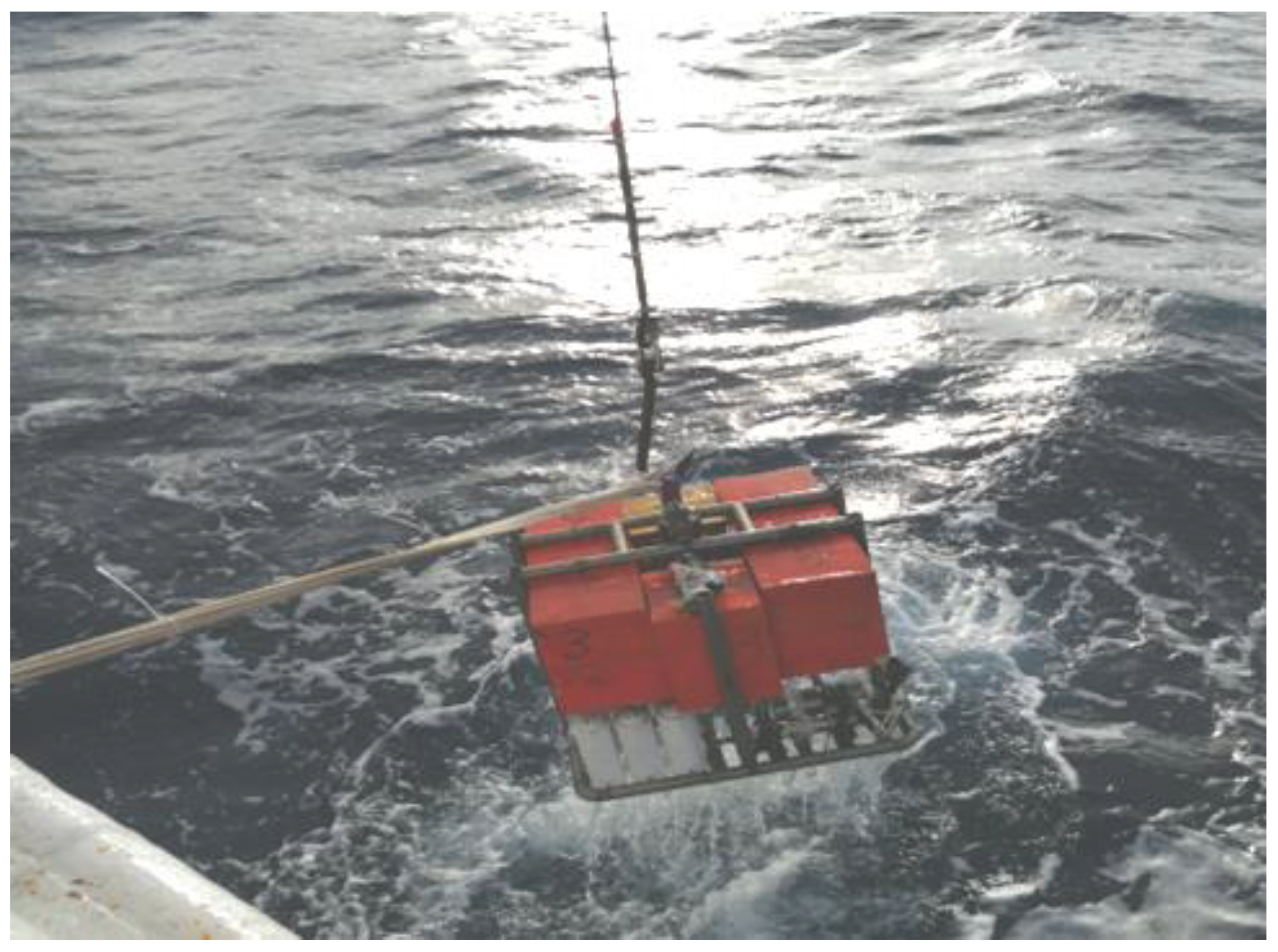
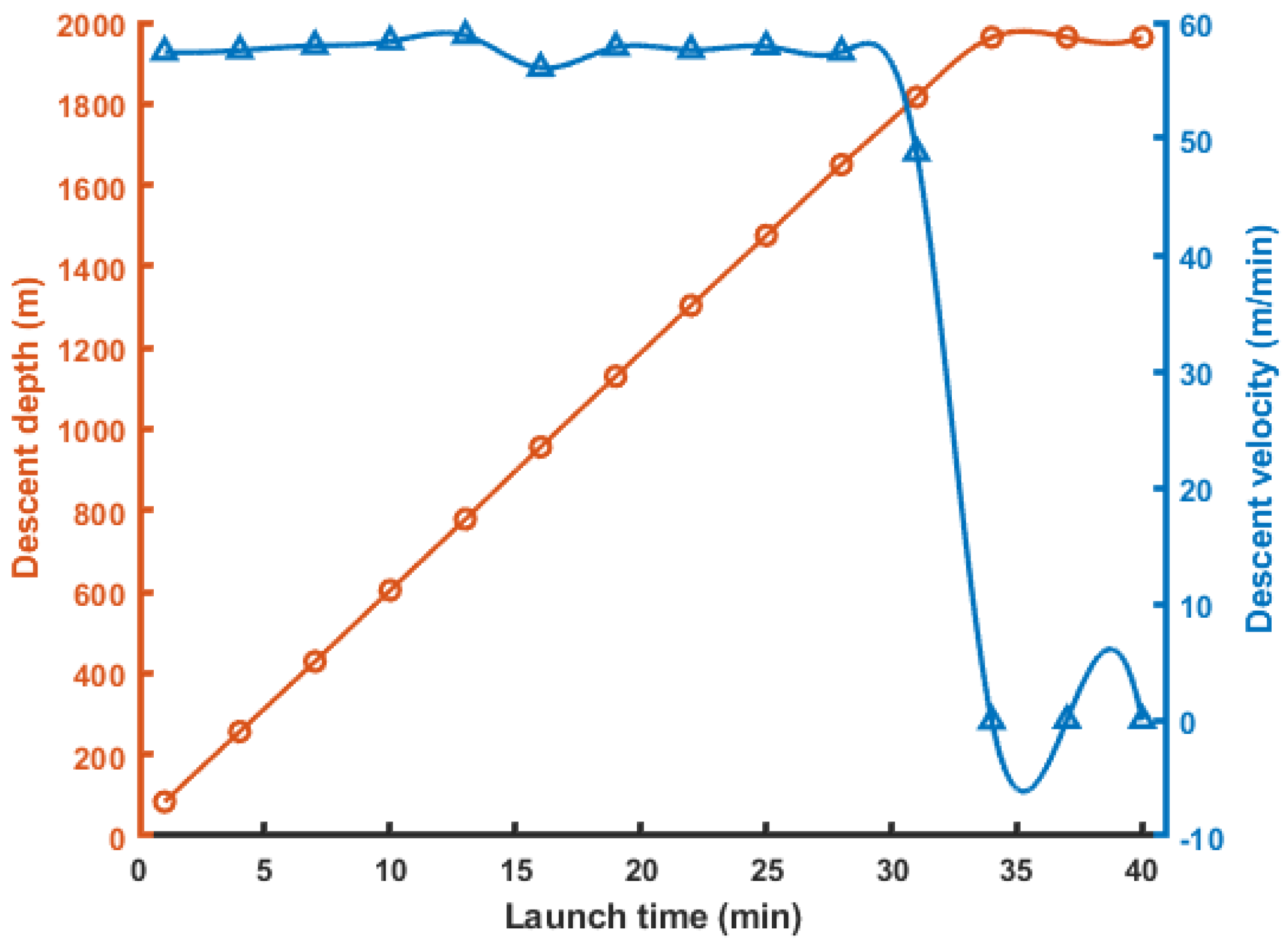
4.2.1. The Water Entry Process of the Benthic Lander
4.2.2. The Recovery Process of the Benthic Lander
5. Conclusions
Author Contributions
Funding
Institutional Review Board Statement
Informed Consent Statement
Data Availability Statement
Conflicts of Interest
Appendix A

| Load (N) | Principal Stress (Mpa) | Principal Strain (mm/mm) | Equivalent Stress (Mpa) | Equivalent Strain (mm/mm) | Total Deformation (mm) | Total Deformation Energy (MJ) |
|---|---|---|---|---|---|---|
| 5000 | 9.4133 | 9.65 × 10⁻⁵ | 11.09 | 1.16 × 10⁻⁴ | 0.44 | 387.75 |
| 7500 | 14.12 | 1.45 × 10⁻⁴ | 16.636 | 1.74 × 10⁻⁴ | 0.66 | 872.44 |
| 10,000 | 18.827 | 1.93 × 10⁻⁴ | 22.181 | 2.31 × 10⁻⁴ | 0.88 | 1551 |
| 12,500 | 23.533 | 2.41 × 10⁻⁴ | 27.726 | 2.89 × 10⁻⁴ | 1.11 | 2423.4 |
| 15,000 | 28.24 | 2.90 × 10⁻⁴ | 33.271 | 3.47 × 10⁻⁴ | 1.33 | 3489.8 |
| 20,000 | 37.653 | 3.86 × 10⁻⁴ | 44.361 | 4.63 × 10⁻⁴ | 1.77 | 6204 |
| Load (N) | Principal Stress (Mpa) | Principal Strain (mm/mm) | Equivalent Stress (Mpa) | Equivalent Strain (mm/mm) | Total Deformation (mm) | Total Deformation Energy (MJ) |
|---|---|---|---|---|---|---|
| 5000 | 0.41005 | 3.42 × 10⁻⁶ | 0.96429 | 9.42 × 10⁻⁶ | 3.10 × 10⁻² | 44.295 |
| 7500 | 0.61507 | 5.13 × 10⁻⁶ | 1.3564 | 1.41 × 10⁻⁵ | 4.65 × 10⁻² | 99.664 |
| 10,000 | 0.8201 | 6.84 × 10⁻⁶ | 1.8186 | 1.88 × 10⁻⁵ | 6.19 × 10⁻² | 177.18 |
| 12,500 | 1.0251 | 8.55 × 10⁻⁶ | 2.2607 | 2.36 × 10⁻⁵ | 7.74 × 10⁻² | 276.84 |
| 15,000 | 1.2301 | 1.03 × 10⁻⁵ | 2.7129 | 2.83 × 10⁻⁵ | 9.29 × 10⁻² | 398.66 |
| 20,000 | 1.6402 | 1.37 × 10⁻⁵ | 3.6172 | 3.77 × 10⁻⁵ | 1.24 × 10⁻¹ | 708.72 |
| Load (N) | Principal Stress (Mpa) | Principal Strain (mm/mm) | Equivalent Stress (Mpa) | Equivalent Strain (mm/mm) | Total Deformation (mm) | Total Deformation Energy (MJ) |
|---|---|---|---|---|---|---|
| 5000 | 2.8473 | 2.93 × 10⁻⁵ | 2.927 | 3.06 × 10⁻⁵ | 0.15 | 139.88 |
| 7500 | 4.271 | 4.40 × 10⁻⁵ | 4.3904 | 4.59 × 10⁻⁵ | 0.22 | 314.72 |
| 10,000 | 5.6957 | 5.86 × 10⁻⁵ | 5.8539 | 6.12 × 10⁻⁵ | 0.30 | 559.5 |
| 12,500 | 7.1183 | 7.33 × 10⁻⁵ | 7.3174 | 7.65 × 10⁻⁵ | 0.37 | 874.23 |
| 15,000 | 8.542 | 8.80 × 10⁻⁵ | 8.7809 | 9.18 × 10⁻⁵ | 0.45 | 1258.9 |
| 20,000 | 11.389 | 1.17 × 10⁻⁴ | 11.708 | 1.22 × 10⁻⁴ | 0.60 | 2238.0 |
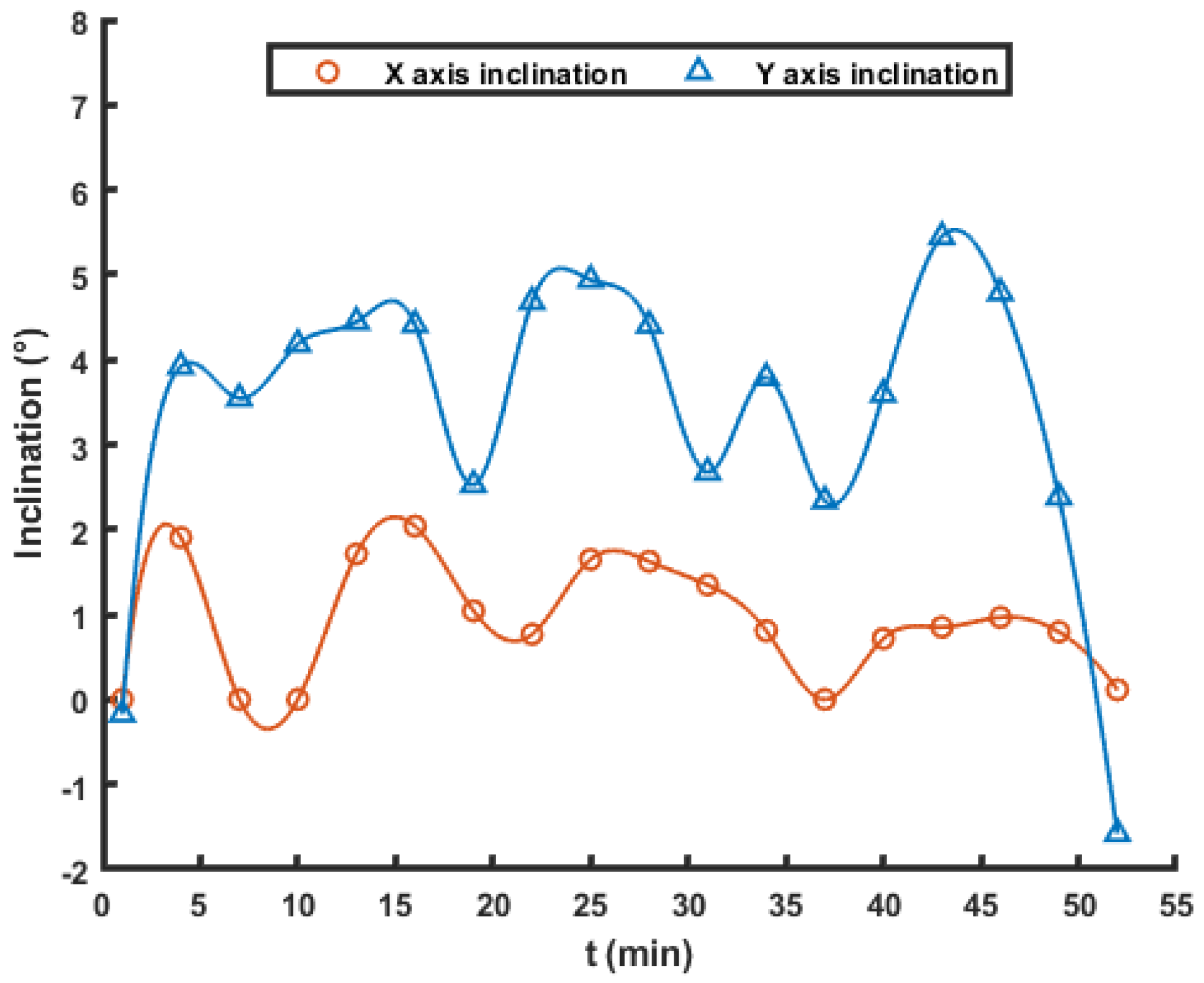
| Time (min) | Depth (m) | X Axis Inclination (°) | Y Axis Inclination (°) | Time (min) | Depth (m) | X Axis Inclination (°) | Y Axis Inclination (°) |
|---|---|---|---|---|---|---|---|
| 1 | 83.6 | 0 | −0.1734 | 28 | 1650.1 | 1.625 | 4.4031 |
| 4 | 256.3 | 1.9056 | 3.9195 | 31 | 1816.4 | 1.3477 | 2.6747 |
| 7 | 428.7 | 0 | 3.5445 | 34 | 1963.1 | 0.8087 | 3.7875 |
| 10 | 603.8 | 0 | 4.1818 | 37 | 1963.1 | 0 | 2.3382 |
| 13 | 778.8 | 1.7126 | 4.4433 | 40 | 1963.2 | 0.7155 | 3.5922 |
| 16 | 955.9 | 2.0396 | 4.4114 | 43 | - | 0.851 | 5.4462 |
| 19 | 1129.7 | 1.0428 | 2.5263 | 46 | - | 0.9662 | 4.7874 |
| 22 | 1303.7 | 0.767 | 4.6813 | 49 | - | 0.7953 | 2.3831 |
| 25 | 1476.0 | 1.6482 | 4.9387 | 52 | - | 0.1134 | −1.5809 |
References
- Zhang, X. Quantitative Applications of Raman Technique for Deep-Sea Environment and Sediment Detection. Ph.D. Thesis, Ocean University of China, Qingdao, China, 2009. [Google Scholar]
- Ding, Z.; Ren, Y.; Zhang, Y.; Yang, L.; Dewei, L.I. Research and Prospect of Deep-sea Detection Technology. Ocean. Coast. Manag. 2019, 71–77. [Google Scholar]
- Huaichao, W.U.; Chunyang, T.; Bo, J.; Canjun, Y.; Ying, C. Design of an energy supplying device for equipments for in-situ detection of deep-sea hydrothermal fluid. Haiyang Kexue 2011, 35, 82–85. [Google Scholar]
- Tahey, T.M.; Duineveld, G.C.A.; DeWilde, P.; Berghuis, E.M.; Kok, A. Sediment O-2 demand, density and biomass of the benthos and phytopigments along the northwestern Adriatic coast: The extent of Po enrichment. Oceanol. Acta 1996, 19, 117–130. [Google Scholar]
- Lavaleye, M.; Duineveld, G.; Lundalv, T.; White, M.; Guihen, D.; Kiriakoulakis, K.; Wolff, G.A. Cold-Water Corals on the Tisler Reef: Preliminary Observations on the Dynamic Reef Environment. Oceanography 2009, 22, 76–84. [Google Scholar] [CrossRef] [Green Version]
- Oevelen, D.; Duineveld, G.; Lavaleye, M.; Mienis, F.; Soetaert, K.; Heip, C. The cold-water coral community as hotspot of carbon cycling on continental margins: A food-web analysis from Rockall Bank (northeast Atlantic). Limnol. Oceanogr. 2009, 54, 1829–1844. [Google Scholar] [CrossRef] [Green Version]
- Black, K.S.; Fones, G.R.; Peppe, O.C.; Kennedy, H.A.; Bentaleb, I. An autonomous benthic lander: Preliminary observations from the UK BENBO thematic programme. Cont. Shelf. Res. 2001, 21, 859–877. [Google Scholar] [CrossRef]
- Santana, J.P.; Mathias, N.; Hoveling, R.; Alves, H.; Morais, T. Innovative Benthic Lander for Macroalgae Monitoring in Shallow-Water Environments. J. Marine. Sci. Appl. 2020, 19, 133–147. [Google Scholar] [CrossRef]
- Wheeler, A.J.; Lim, A.; Butschek, F.; O’Reilly, L.; Harris, K.; O’Driscoll, P. The “Little MonSta” Deep-Sea Benthic, Precision Deployable, Multi-Sensor and Sampling Lander Array. Sensors 2021, 21, 3355. [Google Scholar] [CrossRef] [PubMed]
- Linke, P.; Sommer, S.; Rovelli, L.; McGinnis, D.F. Physical limitations of dissolved methane fluxes: The role of bottom-boundary layer processes. Mar. Geol. 2010, 272, 209–222. [Google Scholar] [CrossRef]
- Zheng, M.; Yang, J.; Zhang, P.; Wang, C. A Long-Term Observation of Deep-Sea Environment and Biological Trap; CN105716663A; China National Intellectual Property Administration: Beijing China, 2016.
- Chen, J.; Zhang, Q.F.; Jun, L.I.; Zhang, A.Q. Research on the Application of the Hadal Lander Technology in the Mariana Trench. J. Ocean Technol. 2017, 36, 63–69. [Google Scholar]
- Roegner, G.C.; Fields, S.A.; Henkel, S.K. Benthic video landers reveal impacts of dredged sediment deposition events on mobile epifauna are acute but transitory. J. Exp. Mar. Biol. Ecol. 2021, 538, 151526. [Google Scholar] [CrossRef]
- Sun, G.; Zhao, S. Mechanics of Materials; Shanghai Jiao Tong University Press: Shanghai, China, 2015. [Google Scholar]
- Yuan, G. Analysis of Meshing Dirision Method. Mod. Mach. 2009, 59–60. [Google Scholar]
- Gonalves, F.A.; Gomes, M.O.; Mathias, N.; Morais, T.; Ferradosa, T. Numerical modelling of full-scale subsea lander AMALIA with in-situ conditions. Proc. Inst. Civil Eng.-Marit. Eng. 2020, 173, 110–119. [Google Scholar]
- Pelletier, D.; Rouxel, J.; Fauvarque, O.; Hanon, D.; Gestalin, J.-P.; Lebot, M.; Dreano, P.; Furet, E.; Tardivel, M.; Le Bras, Y.; et al. KOSMOS: An Open Source Underwater Video Lander for Monitoring Coastal Fishes and Habitats. Sensors 2021, 21, 7724. [Google Scholar] [CrossRef] [PubMed]
- Spagnoli, F.; Penna, P.; Giuliani, G.; Masini, L.; Martinotti, V. The AMERIGO Lander and the Automatic Benthic Chamber (CBA): Two New Instruments to Measure Benthic Fluxes of Dissolved Chemical Species. Sensors 2019, 19, 2632. [Google Scholar] [CrossRef] [PubMed] [Green Version]
- Peoples, L.M.; Norenberg, M.; Price, D.; McGoldrick, M.; Novotny, M.; Bochdansky, A.; Bartlett, D.H. A full-ocean-depth rated modular lander and pressure-retaining sampler capable of collecting hadal-endemic microbes under in situ conditions—ScienceDirect. Deep-Sea Res. I Oceanogr. Res. Pap. 2019, 143, 50–57. [Google Scholar] [CrossRef]


| Material Parameters | Sediment | Benthic Lander (Titanium Alloy) |
|---|---|---|
| Density (kg/m3) | 1.35 × 10³ | 4.5 × 10³ |
| Elastic modulus (MPa) | 1.24 × 10⁵ | 1.8 |
| Poisson’s ratio | 0.3 | 0.33 |
| Shear modulus (kPa) | 5.5 | 4.7 × 10⁷ |
| Internal friction angle (°) | 3.1 | - |
| Cohesion (kPa) | 12.6 | - |
| Deformation Index | 0.56 | - |
| Cohesive deformation modulus | 0.68 | - |
| 0.5 m/s | 0.7 m/s | 1.0 m/s | 1.2 m/s | 1.5 m/s | |
|---|---|---|---|---|---|
| Square pillar | 8.25 | 11.60 | 16.63 | 19.98 | 25.02 |
| Round pillar | 8.23 | 11.29 | 16.17 | 19.43 | 24.32 |
| No pillars | 8.65 | 12.15 | 17.42 | 20.94 | 26.23 |
| 0.5 m/s | 0.7 m/s | 1.0 m/s | 1.2 m/s | 1.5 m/s | |
|---|---|---|---|---|---|
| Square pillar | 7.02 × 10⁻² | 9.85 × 10⁻² | 1.78 × 10⁻¹ | 2.57 × 10⁻¹ | 4.04 × 10⁻¹ |
| Round pillar | 7.41 × 10⁻² | 1.04 × 10⁻¹ | 1.49 × 10⁻¹ | 2.09 × 10⁻¹ | 3.37 × 10⁻¹ |
| No pillars | 1.85 × 10⁻¹ | 3.66 × 10⁻¹ | 7.65 × 10⁻¹ | 1.11 | 1.76 |
| Initial Speed of Collision (m/s) | 0.5 | 0.7 | 1.0 | 1.2 | 1.5 |
| Maximum Subsidence Depth (mm) | 18 | 23.8 | 32.5 | 39.5 | 50 |
| Two Points Taken | (a, b) | Total Error | Variance |
|---|---|---|---|
| 1, 2 | (29, 3.5) | 4.2 | 10.44 |
| 1, 3 | (29, 3.5) | 4.2 | 10.44 |
| 1, 4 | (30.7, 2.65) | 2.49 | 2.5026 |
| 1, 5 | (32, 2) | 3 | 3.42 |
Publisher’s Note: MDPI stays neutral with regard to jurisdictional claims in published maps and institutional affiliations. |
© 2022 by the authors. Licensee MDPI, Basel, Switzerland. This article is an open access article distributed under the terms and conditions of the Creative Commons Attribution (CC BY) license (https://creativecommons.org/licenses/by/4.0/).
Share and Cite
Yu, Z.; Zhang, C.; Chen, J.; Ren, Z. Dynamic Analysis of Bottom Subsidence of Benthic Lander. J. Mar. Sci. Eng. 2022, 10, 824. https://doi.org/10.3390/jmse10060824
Yu Z, Zhang C, Chen J, Ren Z. Dynamic Analysis of Bottom Subsidence of Benthic Lander. Journal of Marine Science and Engineering. 2022; 10(6):824. https://doi.org/10.3390/jmse10060824
Chicago/Turabian StyleYu, Zhou, Chunyue Zhang, Jiawang Chen, and Ziqiang Ren. 2022. "Dynamic Analysis of Bottom Subsidence of Benthic Lander" Journal of Marine Science and Engineering 10, no. 6: 824. https://doi.org/10.3390/jmse10060824
APA StyleYu, Z., Zhang, C., Chen, J., & Ren, Z. (2022). Dynamic Analysis of Bottom Subsidence of Benthic Lander. Journal of Marine Science and Engineering, 10(6), 824. https://doi.org/10.3390/jmse10060824