The Influence of Bathymetry on Regional Marine Geoid Modeling in Northern Europe

Abstract

Although Northern Europe has been the target area in many regionwide geoid determination studies, the research has been land-focused, neglecting bathymetry information. With new projects, such as the Baltic Sea Chart Datum 2000, the attention is shifting toward the marine geoid. Hence, consideration for bathymetry has become relevant, the influence of which is studied. In the relatively shallow Baltic Sea, accounting for bathymetry-based residual terrain model reduction during gravity data processing induces marine geoid modeling differences (relative to neglecting bathymetry) mainly within 2 cm. However, the models can deviate up to 3–4 cm in some regions. Rugged Norwegian coastal areas, on the other hand, had modeling improvements around a decimeter. Considering bathymetry may thus help improve geoid modeling outcomes in future Northern Europe geoid determination projects. Besides using the conventional precise GNSS-leveling control points, the paper also demonstrates the usefulness of shipborne GNSS and airborne laser scanning-derived geoidal heights in validating geoid modeling results. A total of 70 gravimetric geoid solutions are presented, for instance, by varying the used reference global geopotential models. According to the comparisons, GOCO05c-based solutions generally perform the best, where modeling agreement with GNSS-leveling control points reached 2.9 cm (standard deviation) from a one-dimensional fit.

1. Introduction

Determination of accurate marine (quasi)geoid models is essential for geodetic and engineering applications but can also be required in oceanographic research (over marine areas, the geoid coincides with the quasigeoid; henceforth, the shorter term will be primarily used). The advances in satellite gravimetry (e.g., the use of GRACE and GOCE missions’ data) allow us to solve the marine geoid with an accuracy of a few centimeters for longer wavelengths [1,2]. Due to omission errors, however, global geopotential models (GGMs) may be insufficient for regional-scale applications. For example, centimeter-level geoid modeling accuracy is required for GNSS (global navigation satellite system)-based height determination in engineering and navigation, especially near coastal areas. Additionally, improving coastal mean dynamic topography estimates [3,4] and detecting significant mean dynamic topography signals on smaller spatial scales [5,6] require more precise marine geoid models than GGMs. Thus, methods for regional geoid determination need to be employed to improve marine geoid models for shorter wavelengths.

Gravimetric geoid models can be computed, for instance, by Stokes’s formula [7], which enables the determination of models from globally distributed gravity anomalies. Since such an approach is unfeasible in practice, the integration can be limited to a smaller spatial domain around the computation points. The resulting truncation error (due to neglecting the far zone) can be reduced by modifying Stokes’s formula [8], allowing terrestrial gravity anomalies to be combined with a suitable satellite-derived GGM. The latter provides the long-wavelength component of the geoid. Two primary groups of Stokes’s formula modifications exist: deterministic and stochastic methods. Deterministic modification methods aim to reduce the truncation error only. On the other hand, stochastic methods also attempt to reduce errors in terrestrial gravity anomalies and GGMs. For further details and comparisons between these modification methods, see [9,10,11]. This study employs the least-squares modification of Stokes’s formula with additive corrections (LSMSA) [12,13] for geoid modeling, which uses stochastic modification.

The above-described approach is only one possibility for regional geoid determination, and other alternatives exist (e.g., the remove–compute–restore technique and least-squares collocation), whereby various computation methods may result in similar modeling accuracies [14]. Instead, the geoid modeling outcome can be influenced more significantly by the quality and processing of the input gravity data [15]. Although methods for geoid determination from discrete gravity data exist [16,17], a regular grid of gravity anomalies is usually required. Thus, a suitable gravity data gridding approach also needs to be selected. Due to terrain and bathymetry correlated high-frequency gravity field variations, the direct gridding of surface gravity anomalies is usually unreliable since it is difficult for interpolation algorithms to estimate correct gravity values at the grid nodes. The remove–solve–restore procedure can be used instead, meaning that the gravity anomalies are reduced to some smoother alternative (e.g., Bouguer or residual terrain model (RTM) anomalies), gridded and then restored [15]. Such an approach allows a more reliable prediction of gravity values but can also add gravity information to data void areas during the signal restoration. A digital terrain model (DTM) is essential for estimating the high-frequency gravity field component, which needs to be removed from the discrete points and restored on the gridded gravity dataset [18]. Although the initial gravity anomalies are smoother in marine areas, it could be advantageous also to consider bathymetry information besides a DTM for marine geoid modeling.

Several regionwide geoid modeling projects have been conducted in the Baltic Sea region in Northern Europe [15,18,19,20,21,22,23,24,25,26,27,28,29], with the primary focus on land areas. No bathymetry information was considered in these projects. However, it was shown by [30] that consideration for bathymetry could significantly influence geoid modeling outcomes in the Norwegian fjords. The focus has now shifted from land to the marine geoid. Implementation of the Baltic Sea Chart Datum 2000 (BSCD2000), a common height reference for the Baltic Sea region, has been initiated to effectively use GNSS methods for accurate navigation and real-time offshore surveying [31,32]. The BSCD2000 will be realized through GNSS and geoid modeling. This paper details the Tallinn University of Technology’s (one of the BSCD2000 computation centers) geoid modeling efforts toward realizing BSCD2000. Since the focus is now on the marine geoid, it can be of interest how consideration for bathymetry affects the (regular) gravity field estimation and subsequent geoid modeling outcomes. This contribution also aims to investigate these influences in the Baltic Sea region.

An essential component of geoid determination studies is the validation of modeling results. Conventionally, precise GNSS-leveling control points are used, but such validation datasets are limited only to land areas, and no information about the offshore modeling performance is retrieved. The shipborne GNSS [33,34,35] and airborne laser scanning [36,37,38] measured sea surface heights may provide valuable knowledge about the marine geoid instead. By removing the ever-changing dynamic topography, for instance, using hydrodynamic models and tide gauge data [35,38,39], the sea surface heights can be reduced to geoidal heights. This study demonstrates how such marine datasets can help evaluate various gravimetric geoid modeling solutions, especially if the aim is to model the marine geoid.

The structure of the paper is as follows. Section 2 describes the gravity data processing and geoid modeling approaches. Note that in this study, quasigeoid is being modeled; thus, in Section 2, the focus is on quasigeoid-associated values. The subsequent Section 3 introduces the study area and gives an overview of the used data. Section 4 then presents the results of the gravity data gridding and geoid modeling. The influence of bathymetry information is investigated, and various geoid modeling solutions are evaluated. The paper continues with a discussion in Section 5 and ends with a summary in Section 6.

2. Methods

2.1. From Discrete Gravity Data to a Gridded Gravity Field Representation

The measured gravity value $g_P$ on or above terrain (or sea surface) at point $P$ (at a normal height $H_P^{*}$ relative to the quasigeoid) can be reduced to the surface free-air anomaly:

$$\Delta g_P^{FAA}=g_P-{\gamma }_Q,$$

(1)

where ${\gamma }_Q$ is the normal gravity at point $Q$ (at height $h_Q=H_P^{*}$ above the GRS80 reference ellipsoid) on the telluroid. According to [40], the normal gravity ${\gamma }_Q$ can be approximated as:

$${\gamma }_Q\approx {\gamma }_0-\frac{2{\gamma }_e}{a}\left[1+f+m+\left(-3f+\frac{5}{2}m\right){\sin }^2\phi \right]H_P^{*}+\frac{3{\gamma }_e}{a^2}{H}_P^{*}{}^2,$$

(2)

where ${\gamma }_0$ and $\phi$ are the normal gravity on the reference ellipsoid and the geodetic latitude of point $P$, respectively. The former is defined as:

$${\gamma }_0={\gamma }_e\frac{1+k{\sin }^2\phi }{\sqrt{1-e^2{\sin }^2\phi }}.$$

(3)

Terms ${\gamma }_e$ (normal gravity at equator), $a$ (equatorial radius), $f$ (flattening), $m\approx {\omega }^{2}a/{\gamma }_e$ ($\omega$ is angular velocity), $k=b{\gamma }_p/a{\gamma }_e-1$ ($b$ and ${\gamma }_p$ are polar radius and normal gravity at pole, respectively) and $e$ (first eccentricity) in Equations (2) and (3) are parameters associated with the GRS80 reference ellipsoid [41]. From the obtained surface free-air anomalies $\Delta g_P^{FAA}$ at discrete locations $P$, a regular grid needs to be estimated for geoid modeling purposes. However, since surface free-air anomalies contain terrain and bathymetry correlated high-frequency gravity field variations, direct gridding of these data may provide unreliable results. A reduction in these values to a smoother alternative is thus required.

To improve data gridding performance, implementing the concept of a band-bass filter that attenuates gravity signals above and below desired frequency could be beneficial. Such an approach allows the derivation of RTM anomalies:

$$\Delta g_P^{RTMA}=\Delta g_P^{FAA}-\Delta g_P^{GGM}-\delta g_P^{RTM},$$

(4)

where $\Delta g_P^{GGM}$ represents the long-wavelength component from a GGM evaluated to a suitable degree and order (d/o). The term $\delta g_P^{RTM}$, on the other hand, represents the short-wavelength topographic effect of RTM reduction estimated from a DTM (and/or bathymetry model). The RTM reduction can be computed as:

$$\delta g_P^{RTM}=2\pi G\rho \left(H_P^{*}-H_P^{ref}\right)-\left({\delta g_P^T |}_{z_1=H_P^{*}}^{z_2=H^{*}}-{\delta g_P^T |}_{z_1=H_P^{ref}}^{z_2=H^{ref}}\right),$$

(5)

where $\delta g_P^T$ is the terrain correction estimated by summing the attraction of a finite number of rectangular prisms according to [42,43]:

$$\delta g_P^T=-G{{\displaystyle \sum }}^{ }\underset{x_1}{\overset{x_2}{{\displaystyle \int }}}\underset{y_1}{\overset{y_2}{{\displaystyle \int }}}\underset{z_1}{\overset{z_2}{{\displaystyle \int }}}\frac{\rho \left(z-z_P\right)}{{\left[{\left(x-x_P\right)}^2+{\left(y-y_P\right)}^2+{\left(z-z_P\right)}^2\right]}^{3/2}}dxdydz,$$

(6)

where $x_P$, $y_P$, $z_P$ and $x$, $y$, $z$ are the local Cartesian coordinates of the computation point $P$ and the moving integration element, respectively, with $x_1$, $x_2$, $y_1$, $y_2$, $z_1$, and $z_2$ defining the sizes of prisms. In Equations (5) and (6), the term $G$ denotes the gravitational constant and $\rho$ topographic density. The latter can be assumed at 2670 kg/m³ for terrain and 1640 kg/m³ for bathymetry (i.e., the difference between terrain and seawater densities). Note that in Equation (5), terms $H_P^{*}$ and $H^{*}$ represent normal heights of the computation point $P$ and moving integration element (determined from a DTM), respectively. The terms $H_P^{ref}$ and $H^{ref}$ are correspondingly normal heights of a smooth reference surface, which can be constructed by low-pass filtering the used DTM. Ideally, the resolution of the reference surface should correspond to the d/o of the used GGM since RTM reduction aims to remove the remaining higher-frequency gravity contribution beyond that d/o. The described RTM reduction is implemented in sub-program TC [43] of the GRAVSOFT research software package.

Generally, marine gravity is measured along relatively sparse parallel tracks, whereby gaps in data coverage are also common. It has been demonstrated that least-squares collocation (LSC) can provide reliable gridding results for such data [15]. Provided that gravity data have reliable a priori error estimates, LSC using RTM anomalies can also result in high-quality gravity field representation in areas with dense gravity data coverage [15]. With the weighted LSC method, the RTM anomaly values $\Delta g_G^{RTMA}$ at grid nodes are predicted from discrete values $\Delta g_P^{RTMA}$ at locations $P$ according to [44] by solving the following matrix equation:

$$\Delta g_G^{RTMA}=C_{st}{\left(C_{tt}+C_{nn}\right)}^{-1}\Delta g_P^{RTMA},$$

(7)

where $C_{st}$ is the cross-covariance matrix of the predicted ($\Delta g_G^{RTMA}$) and known ($\Delta g_P^{RTMA}$) signals and $C_{tt}$ and $C_{nn}$ are the covariance matrixes of known signal and observation errors, respectively. Since $\Delta g_P^{RTMA}=t+n$, the covariance matrix of observed values at discrete locations is $C_{g_P^{RTMA}{g}_P^{RTMA}}=C_{tt}+C_{nn}$. The LSC method is implemented in the GRAVSOFT sub-program GEOGRID.

For such a gridding approach, covariance matrixes estimated from survey data describe the data spatial dependence by fitting a theoretical model to the empirical covariance values. In this study, the second-order Markov covariance model [45] was used:

$$C\left(l\right)=C_0\left(1+\frac{l}{\alpha }\right)e^{-l/\alpha },$$

(8)

where $C\left(l\right)$ is the modeled covariance value over the distance $l$, $C_0$ is the signal variance and $\alpha$ is a parameter related to the correlation length $X_{1/2}$ as $\alpha \approx 0.595X_{1/2}$. The correlation length is defined as the distance at which the covariance function reaches half the value of $C_0$.

To finally obtain the gridded surface free-air anomalies, the previously removed long- and short-wavelength gravity contributions can be restored on the gridded RTM anomalies:

$$\Delta g_G^{FAA}=\Delta g_G^{RTMA}+\Delta g_G^{GGM}+\delta g_G^{RTM},$$

(9)

where $\Delta g_G^{GGM}$ and $\delta g_G^{RTM}$ are now computed at the locations of grid nodes. The long- and short-wavelength gravity signals estimated from a GGM and DTM, respectively, can hence also provide information at the locations of previously existing data voids. A high-quality DTM may thus significantly enhance the gravity field estimation, improving the accuracy of subsequent geoid modeling (a bathymetry model may have a similar influence).

2.2. Quasigeoid Determination

Geoidal heights can be approximated using the unbiased LSMSA geoid modeling approach [12,46] with the gridded surface free-air anomalies:

$$\tilde{N}=\frac{R}{4\pi {\gamma }_0}{\displaystyle {{\displaystyle \iint }}_{{\sigma }_0}}{S}^L\left(\psi \right)\Delta g_G^{FAA}d\sigma +\frac{R}{2{\gamma }_0}{\displaystyle \sum }_{n=2}^M\left(s_n+Q_n^L\right)\Delta g_n^{GGM},$$

(10)

where $R$ is the mean Earth radius, $S^L\left(\psi \right)$ is the Stokes’s function modified up to the degree limit $L$ and $\psi$ denotes a geocentric angle between computation and moving integration points. Integration is limited to a spherical cap ${\sigma }_0$ (with geocentric angle ${\psi }_0$) around a computation point. The modified Stokes’s function is:

$$S^L\left(\psi \right)={\displaystyle \sum }_{n=2}^{\infty }\frac{2n+1}{n-1}{P}_n\left(\cos \psi \right)-{\displaystyle \sum }_{n=2}^L\frac{2n+1}{2}{s}_n{P}_n\left(\cos \psi \right),$$

(11)

where the first term denotes the original Stokes’s function $S\left(\psi \right)$ and $P_n\left(\cos \psi \right)$ Legendre polynomial of degree $n$. The modification parameters $s_n$ in Equations (10) and (11) are solved from a linear system of equations in the least-squares sense [12]. These were estimated as described in [47,48]. Since the unbiased LSMSA approach leads to an ill-conditioned system of linear equations, singular value decomposition was used to ensure the solution’s stability. The terrestrial gravity data uncertainties were assumed at 2 mGal as the focus is on marine areas where gravity data noise is more significant (due to dynamic measuring conditions) than on land (generally in the range of 0.5–1 mGal).

The modified truncation coefficients $Q_n^L$ in Equation (10) are computed as:

$$Q_n^L=Q_n^L\left({\psi }_0\right)=Q_n\left({\psi }_0\right)-{\displaystyle \sum }_{k=2}^L\frac{2k+1}{2}{s}_k{R}_{nk}\left({\psi }_0\right).$$

(12)

Molodenskii’s truncation coefficients $Q_n$ and coefficients $R_{nk}$ (both a function of ${\psi }_0$) can be evaluated using recursive algorithms given by [49,50]. By employing a suitable GGM up to the degree $M$, Laplace harmonics $\Delta g_n^{GGM}$ in Equation (10) can be computed as:

$$\Delta g_n^{GGM}=\frac{GM}{r^2}{\left(\frac{a}{r}\right)}^n\left(n-1\right){\displaystyle \sum }_{m=0}^n\left(\Delta {\overline{C}}_{nm}\cos m\lambda +{\overline{S}}_{nm}\sin m\lambda \right){\overline{P}}_{nm}\left(\cos \theta \right),$$

(13)

where $\Delta {\overline{C}}_{nm}$ and ${\overline{S}}_{nm}$ are fully normalized spherical harmonic coefficients of the disturbing potential (relative to the GRS80 reference ellipsoid). Note that modification limits $M$ and $L$ are consistently selected as equal in this study. Term $GM$ is the terrestrial gravitational constant, $a$ is the equatorial radius, $r$, $\lambda$ and $\theta$ are spherical geocentric radius, longitude and co-latitude, respectively, and ${\overline{P}}_{nm}\left(\cos \theta \right)$ denotes fully normalized Legendre functions.

With the geoid estimator $\tilde{N}$ computed, height anomalies (i.e., quasigeoid heights) can be determined:

$$\zeta =\tilde{N}+\delta {\zeta }_{DWC}+\delta {\zeta }_{ATM}+\delta {\zeta }_{ELL},$$

(14)

where $\delta {\zeta }_{DWC}$ is the combined downward continuation effect [51], $\delta {\zeta }_{ATM}$ is the combined atmospheric effect [52,53,54], and $\delta {\zeta }_{ELL}$ is the combined ellipsoidal effect [55,56,57] (i.e., the additive corrections). The equations for these effects are explicitly spelled out in [58] and are thus not repeated here. Importantly, the presented investigations neglect consideration for atmospheric and ellipsoidal effects due to their relatively small magnitude (generally sub-centimeter; see numerical examples in [58,59,60]). Since these effects are also computed independently of surface free-air anomalies, they do not affect the examination of bathymetry contribution to geoid modeling outcomes (i.e., their influence cancels out in comparisons). The combined downward continuation effect, on the other hand, requires knowledge of the vertical gradients of surface free-air anomalies (estimated using GRAVSOFT sub-program GEOFOUR) and has a magnitude up to a few decimeters (in the study area).

3. Study Area and Data

In the BSCD2000 project, the geoid modeling target area extends from 53° N to 66.5° N and 8.5° E to 31° E (cf. Figure 1), whereby the modeling resolution is 0.01° × 0.02°. The defined extents cover the whole Baltic Sea and its surrounding areas. For modeling the BSCD2000 geoid, a dataset of surface free-air anomalies (Figure 2) was provided in the zero-tide permanent tide concept (see [61,62] for details about permanent tide concepts). This study uses the final version 3 of the database release. These gravity data cover the area from 52° N to 67.5° N and 5.5° E to 34° E. Comparison between Figure 1 and Figure 2 shows that the surface free-air anomalies are highly correlated with rugged terrain (notice Norway and Sweden) and thus ill-suited for gridding.

To reduce surface free-air anomalies to RTM anomalies, which are more suitable for gridding, a DTM is required. For the BSCD2000 geoid modeling project, a section of the 3″ × 3″ NKG-DEM2014 was provided. The same model has previously been used in modeling the NKG2015 quasigeoid [15,27,29]. For the current study, the model was averaged to 0.001° × 0.002° (i.e., 3.6″ × 7.2″) and 0.01° × 0.02° grids covering the area from 51° N to 68.5° N and 2.5° E to 37° E. These datasets were used in geoid modeling solutions that neglected bathymetry information during RTM computations. The coarse grid with elevations above zero is also required for geoid determination using the LSMSA approach.

An alternative elevation model was also constructed since the NKG-DEM2014 does not contain any bathymetry information (i.e., marine areas have zero elevations). As the primary bathymetry data source, the 15″ × 15″ GEBCO_2021 grid [63] was used. Employing multibeam and single-beam shipborne bathymetry data for validation, ref [64] suggested that the GEBCO_2020 grid (i.e., the previous version) has an accuracy of 58 m (in terms of standard deviation) in the Arctic Ocean (northwest from the study area), where the average depth of the investigated region was around 2500 m. A multibeam bathymetry dataset was used to complement the GEBCO_2021 grid in the Estonian marine areas (notice the dashed blue line surrounding Estonia in Figure 1), obtained from the Estonian Maritime Administration. The dataset is primarily a 3.6″ × 3.6″ grid but also contains some dense scattered data points. A comparison between the GEBCO_2021 and Estonian Maritime Administration datasets yielded a standard deviation estimate of 1.9 m, indicating adequate accuracy of the GEBCO_2021 grid in the Baltic Sea. However, it should be noted that the differences reach up to 10–30 m range in some regions, generally where depth changes are steep. Such differences are likely due to the lower resolution of the GEBCO_2021 grid (i.e., seabed details are not well-captured). All these bathymetry data were jointly resampled to a 3″ × 3″ grid and then subtracted from the NKG-DEM2014. The resulting model was then averaged to 0.001° × 0.002° and 0.01° × 0.02° grids (Figure 1 presents the coarse grid). These datasets were used in geoid modeling solutions that considered bathymetry information during RTM computations.

It is evident from Figure 1 that the Baltic Sea is relatively shallow, having a mean depth of only 54 m and a maximum depth of 459 m [65]. On the other hand, the regions in the northwestern section of the study area at the Norwegian Sea are much deeper, with depths exceeding 2000 m. An essential measure for examining bathymetry’s influence on gravity data processing and geoid modeling is the ruggedness of bathymetry. The terrain ruggedness index (describes elevation differences between adjacent cells of a DTM) developed by [66] was modified for the current study. The modified index is named the bathymetry ruggedness index and computed as:

$$BR{I}_P=\frac{1}{I}{\displaystyle \sum }_{i=1}^I\left|H_i^{*}-H_P^{*}\right|·\left(1-\sqrt{d_i/d_{LIM}}\right),$$

(15)

where $H_P^{*}$ is depth at a computation point $P$, and $H_i^{*}$ represents depth at a data point $i$ with a distance $d_i$ from the computation point. The term $I$ is the total number of data points within the specified radius $d_{LIM}$. The parameter $d_{LIM}$ behaves as a low-pass filter, where the increasing value yields smoother bathymetry ruggedness index features.

The bathymetry ruggedness index (Figure 3 shows the computation results) was computed on a 0.01° × 0.02° grid using the GEBCO_2021 and Estonian Maritime Administration bathymetry datasets. The computation radius $d_{LIM}$ was set to 10 km for the resulting index features to be (visually) similar to surface free-air anomalies. Although the bathymetry ruggedness index values are somewhat arbitrary, the relative comparisons indicate the locations of smooth bathymetry (e.g., near-zero values in the North Sea) and rugged bathymetry (e.g., coastal areas of Norway and in the Norwegian Sea) effectively. Rugged bathymetry can also contribute to the high-frequency gravity field variations like rugged terrain. Thus, the most notable influence of bathymetry information on the geoid modeling results can be expected near the coastal area of Norway, which is described by the study area’s most rugged bathymetry (cf. Figure 3).

Geoid modeling using modified Stokes’s formula also requires a suitable GGM. This study tested modeling by employing GOCO05c [67,68], GO_CONS_GCF_2_DIR_R6 [69], GOCO06s [70,71] and XGM2019 [72,73] models. While GO_CONS_GCF_2_DIR_R6 and GOCO06s represent satellite-only gravity field models, GOCO05c and XGM2019 are combined models containing additional terrestrial and altimetry-based gravity data. Note that GO_CONS_GCF_2_DIR_R6 is initially given in the tide-free permanent tide concept (the other three use the zero-tide concept) and was thus converted to the zero-tide concept first.

Validation Datasets

A dataset of 1902 precise GNSS-leveling control points (Figure 1) was provided to evaluate the gravimetric geoid modeling solutions (Estonian data are available from [74]). The employed geodetic coordinates and ellipsoidal heights are in the ITRF2008 reference frame and use the zero-tide permanent tide concept. Temporal changes due to the postglacial land uplift in the Baltic Sea region have been reduced to the epoch 2000.0. Leveled normal heights are in the national (European Vertical Reference System based or compatible) height system realizations and use the zero-tide permanent tide concept with uplift epoch 2000.0. If the provided data used a different tide concept or had a different uplift epoch (Danish and German GNSS-leveling data), a conversion to the zero-tide permanent tide concept (relative to the Normaal Amsterdams Peil) and uplift epoch 2000.0 was conducted. The NKG2016LU model [75] was used to correct for the land uplift.

Besides the conventional GNSS-leveling control points, alternative marine datasets were also used to evaluate the results. These include shipborne GNSS and airborne laser scanning measured sea surface heights, which were reduced into geoidal heights using instantaneous dynamic topography estimates. Dynamic topography was estimated by combining hydrodynamic models and tide gauge data [35,38,39]. The datasets include the Sektori shipborne GNSS-determined profiles [76] (Figure 4 left), airborne laser scanning-derived profiles [38] (Figure 4 left) and six campaigns (denoted from C1 to C6) of the Salme shipborne GNSS-determined profiles [35,77] (Figure 4 right) of geoidal heights (converted to the zero-tide permanent tide concept). Such marine datasets can be valuable in validating marine geoid models since GNSS-leveling control points cannot be established over marine areas.

4. Gravity Field Estimation and Geoid Modeling

4.1. Preparation of Gravity Data

Before regular gravity field estimation, additional gravity data processing had to be applied to the dataset of surface free-air anomalies (Figure 2). Besides terrestrial and marine gravity data, the dataset also contains some airborne measurements [78]. Since such gravity values are given at the flight altitude, a downward continuation correction must be applied due to signal attenuation. Then, airborne gravity measurements can be treated as terrestrial data. A straightforward method proposed by [79] can be used, where the correction is estimated as a difference between free-air anomaly values at the flight altitude and surface level using a high-resolution GGM (the method has also been tested and found suitable by [15]). Here, EIGEN-6C4 [80] evaluated to its maximum d/o of 2190 was selected. The estimated correction’s standard deviation and maximum value were 0.49 mGal and 3.32 mGal, respectively. Note that XGM2019e [72,73] was also tested, but the application of EIGEN-6C4-based downward continuation correction yielded slightly better (although statistically insignificant) agreement with the (actual) terrestrial data.

A few obvious outlier points in the dataset were removed by comparing the initial anomalies to a preliminary grid solution (computed following subsequent steps). Otherwise, no specific outlier detection was implemented. It is assumed that through many years of significant effort by participating countries (especially prior to NKG2015 computations; some details are in [15]) that have submitted gravity data, gross errors have been largely removed and data quality has been ensured (for instance, ref [81] describes the Estonian gravity data).

Additional gravity data were derived from the EIGEN-6C4 GGM to improve gridding quality at the study area edges. The model was evaluated to its maximum d/o of 2190 on a regular 0.025° × 0.05° grid. These points were no closer to the existing data than 0.15° and 0.3° in latitude and longitude, respectively. The error estimates for these points were assumed at 6 mGal to comply with the typical accuracy of GGMs over oceans [80]. Regarding a priori error estimates, note that most Norwegian data were associated with pessimistic estimates of 5 mGal, which may result in unwanted gravity field smoothing using the weighted LSC method. Thus, to improve gridding results, the a priori error estimates were set to 1 mGal for Norwegian land data exceeding that limit (marine data were left unchanged). The gravity data associated and updated a priori error estimates are shown in Figure 5.

4.2. Determination of Residual Terrain Model Anomalies

Residual terrain model reduction was computed to reduce surface free-air anomalies, prepared as described in the previous section, into RTM anomalies. Two sets of computations were conducted—one, where bathymetry information was included, and the second, where it was neglected. Smooth reference surfaces for the RTM reduction computations were determined by applying a moving average low-pass filter on the respective elevation models, averaged roughly to the resolution corresponding to the degree 300. Integration using the 0.001° × 0.002° grids was performed over a 15 km distance from computation points and over a 200 km distance using the 0.01° × 0.02° grids. Elevation models on land were locally spline interpolated to fit heights of gravity observations in computation points (models were left unchanged for marine points).

Figure 6 shows RTM reduction as the grid used in the restoration step, computed by including bathymetry information, and Figure 7 demonstrates bathymetry’s contribution to the reduction, obtained as the difference between the two RTM reduction grids. In the Baltic Sea, bathymetry contribution generally remains within 5 mGal, but a more considerable influence can be seen in rougher seabed areas (also refer to Figure 3). Significant bathymetry influence in the 20 mGal range can be observed in the Norwegian Sea and around the Norwegian shoreline, where fjords’ depth information can contribute even up to 50 mGal to the RTM reduction. The Norwegian coast is also where marine RTM reduction appears relatively rough, whereas generally, the reduction is rather smooth compared to how it appears in the land areas, especially in Norway (cf. Figure 6). It can be noticed in Figure 7 that bathymetry information also propagates inland from the coast, which is due to the used integration radiuses.

Besides RTM reduction, computation of RTM anomalies also requires the long-wavelength component from a suitable GGM. The GO_CONS_GCF_2_DIR_R6 model evaluated to its maximum d/o of 300 was used here. After RTM anomalies were computed, a single data point with the smallest a priori error estimate was retained within each 0.01° × 0.02° grid cell to avoid aliasing during gravity gridding. If more than one such point existed, all the potential points were averaged both in value and spatially (note that Figure 5 shows the thinned dataset, whereby Norwegian data were assigned 1 mGal a priori error estimates after thinning).

Figure 8 presents RTM anomalies where bathymetry information was considered during computations. Comparison between Figure 2 and Figure 8 demonstrates that the RTM anomalies are much smoother (notice standard deviation estimates) and less biased (notice mean values) than the initial surface free-air anomalies, and thus better suited for gridding. When bathymetry was neglected during the computation of RTM anomalies, the resulting standard deviation estimate was 10.61 mGal, and the mean value was –0.50 mGal. Therefore, consideration for bathymetry yielded a slightly smoother dataset of RTM anomalies (respective estimates shown in Figure 8 are 10.30 mGal and –0.37 mGal). Note that the GOCO06s model evaluated to its maximum d/o of 300 was also tested in determining RTM anomalies. When bathymetry was considered and neglected in computations, the standard deviation estimates were 10.86 mGal and 11.16 mGal, respectively. The use of GO_CONS_GCF_2_DIR_R6 instead of GOCO06s hence provided considerably smoother datasets of RTM anomalies.

4.3. Gravity Data Gridding

Besides comparing surface free-air and RTM anomalies in Figure 2 and Figure 8, respectively, covariance analysis of these quantities was also conducted (Figure 9). It can be noticed that the autocovariance values of RTM anomalies are smaller, especially at short distances (note the 783.4 mGal² estimate of surface free-air anomalies that describes the first-kilometer distance), indicating that the derived RTM anomalies are smoother than the initial surface free-air anomalies. The relative smoothness of RTM anomalies compared to the surface free-air anomalies (here, the processed and thinned dataset is used, which causes the $19.7 \mathrm{mGal}\ne \sqrt{544.5}=23.3 \mathrm{mGal}$ discrepancy between Figure 2 and Figure 9) is also suggested by the signal variances. Consequently, the smoother RTM anomalies can be spaced sparser to guarantee grid prediction accuracy, whereas the use of surface free-air anomalies would require much denser data. Furthermore, in the case of surface free-air anomalies, the second-order Markov covariance model does not fit the empirical data well. Notice how the model either overestimates (at shorter distances) or underestimates (at longer distances) the data spatial correlation. On the other hand, the second-order Markov models’ better fit for RTM anomalies (i.e., the modeled covariance represents empirical data closely) suggests that good data-gridding performance can be expected. Note that the inclusion/neglect of bathymetry data does not significantly affect the second-order Markov covariance models’ estimation, although some parameter differences exist (cf. Figure 9).

Residual terrain model anomalies were gridded using the weighted LSC method. The second-order Markov covariance models, defined by the estimated correlation lengths and determined signal variances (cf. Figure 9), described data spatial dependence. The LSC prediction was set to use the 10 closest data points in each quadrant around a prediction point for computational efficiency. A minimum of 0.5 mGal a priori error estimate was defined, whereas if a data point was associated with a larger error estimate, specific a priori estimates in Figure 5 were used. Such data gridding resulted in two RTM anomaly grids—one with bathymetry information included and the second where it was neglected during previous RTM reduction computations. Finally, the RTM reduction and long-wavelength GGM effects were restored to obtain gridded surface free-air anomalies. Figure 10 shows the grid where bathymetry was considered during computations, and Figure 11 demonstrates the influence of bathymetry on gravity field estimation, obtained as the difference between the two grids of surface free-air anomalies.

In the Baltic Sea, bathymetry contribution to the gridded surface free-air anomalies generally remains within 2 mGal (Figure 11). Around the same magnitude, the contribution propagates to inland areas due to two reasons. The first reason is differences in computed RTM reductions, described in Section 4.2, which also influence gridding results, and the second one is variation in signal properties, which causes differences in the second-order Markov covariance models (cf. Figure 9). The latter induces up to 3 mGal differences in sparse gravity data areas (refer, e.g., to Figure 8).

There are also some sparse marine locations where bathymetry contribution has resulted in around 4 mGal differences. These are in the central part of the Baltic Sea and the Gulf of Finland, where increased ruggedness of bathymetry can also be observed (cf. Figure 3). In the same magnitude, bathymetry has influenced gravity field estimation in the Norwegian Sea. Importantly, a significant impact of bathymetry on the gridding results can be noticed around the shoreline of Norway, where bathymetry contribution is generally within 20 mGal but can reach up to around 40 mGal in some locations. By comparing Figure 3 and Figure 11, it can be noticed that these significant differences coincide with regions of most rugged bathymetry. The bathymetry ruggedness index is also rather well correlated with the bathymetry contribution to the gridded surface free-air anomalies, yielding a correlation coefficient of 0.78 (all marine areas in the geoid modeling target area were considered; absolute values of bathymetry contribution to gravity anomalies were used). It can be concluded that considering bathymetry in gravity field estimation can help retain valuable short-wavelength gravity information.

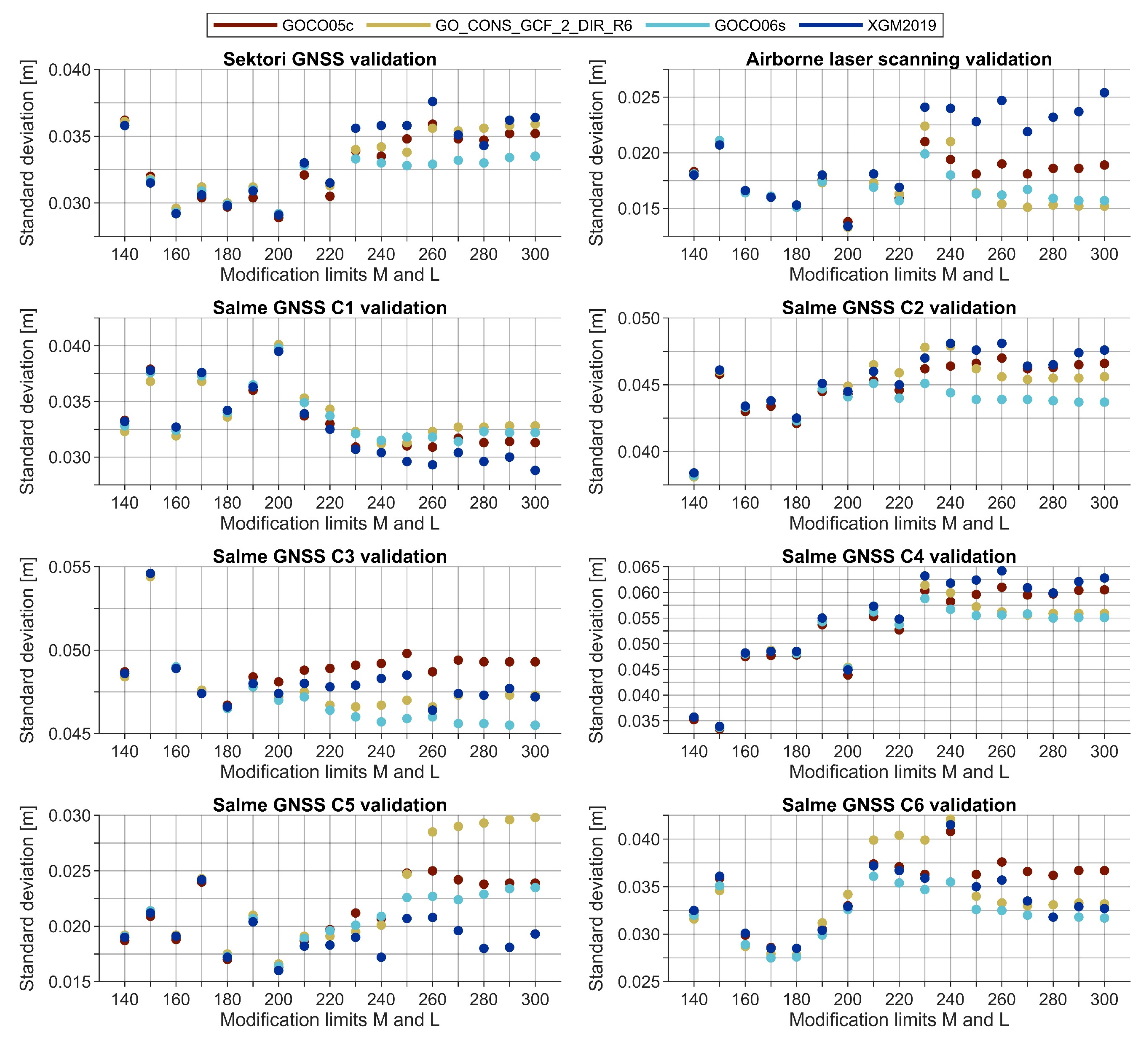
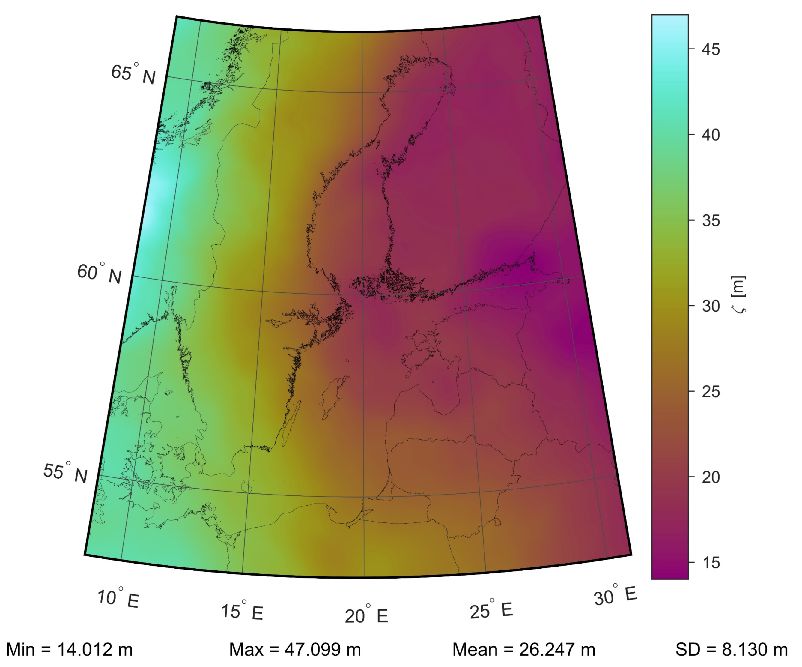
4.4. Results of Geoid Modeling

The surface free-air anomaly grids were employed in geoid determination using the unbiased LSMSA modeling approach. In all computations, integration was limited to 2° (i.e., the geocentric angle ${\psi }_0$). Altogether four GGMs were tested (cf. Section 3), where modification limits (recall that M and L were always set equal) varied between 140 and 300 with an increment of 10. Figure 12 presents validation results based on GNSS-leveling control points (cf. Figure 1), whereby in all these computations, bathymetry information was considered (i.e., the surface free-air anomaly grid where the RTM reduction utilized bathymetry was employed). In the first validation case (upper subplot of Figure 12), a one-dimensional fit was used (i.e., models were directly compared to all GNSS-leveling control points). Since height system biases between countries may exist, in the second validation case (bottom subplot of Figure 12), the control points of each country were first compared with the models separately, and then the residual differences of all countries were considered altogether (i.e., country means were removed).

According to the GNSS-leveling control points, the GOCO05c-based solutions outperform models that use the other three tested GGMs regardless of modification limits. The accuracy (in terms of standard deviation) from a one-dimensional fit reached 2.9 cm with modification limits of 280, whereas limits of 200 yielded an estimate of 2.0 cm when country means were removed from the validation. Up to limits of 220, the GO_CONS_GCF_2_DIR_R6-based solutions appear to show the second-best performance. However, the relative (to other models) accuracy degrades with higher modification limits, where XGM2019-based (the other combined GGM besides GOCO05c) solutions agree better with the GNSS-leveling control points.

The above comparisons only provide information about modeling performance on land, whereas the BSCD2000 project aims to model the marine geoid. Knowledge of the marine geoid’s geometry would thus be valuable. Therefore, a set of marine profiles (cf. Figure 4) was also employed to assess the computed geoid solutions. Figure 13 shows the results of these comparisons, whereby bathymetry information was considered during computations of all the validated models.

In contrast to the comparisons using GNSS-leveling control points, the picture is not as clear with profile-based assessments. For instance, the profiles suggest that the accuracy of modeling solutions based on combined GGMs (GOCO05c and XGM2019) generally degrades with higher modification limits. Contrarily, GOCO06s-based solutions seem to perform the best when limits are high. The agreement between solutions is better with lower modification limits (similarly to the GNSS-leveling comparisons), where GOCO05c-based models perform adequately. It seems that the preferable modification limits could be around 180–200. For example, notice how the comparison with airborne laser scanning profiles (with a total length of 184.4 km) yields an excellent 1.3–1.4 cm agreement (in terms of standard deviation) using modification limits of 200. Interestingly, according to the Salme GNSS C1 profiles, limits of 200 yield the worst results.

It is essential to mention that contrary to GNSS-leveling control points, the profile-based comparisons represent a limited area (cf. Figure 4). Additionally, the accuracy of these marine profiles is most certainly not as high as GNSS-leveling control points. The measurements are conducted in dynamic conditions, but the more crucial issue is that dynamic topography must be estimated to derive geoidal heights from the measured sea surface heights. Due to tide gauge data and hydrodynamic models’ inaccuracies, estimation of instantaneous dynamic topography with an accuracy of a few centimeters is a difficult task. However, even then, such marine profiles can provide beneficial geometric information that can help decision-making in choosing a suitable geoid model out of various solutions.

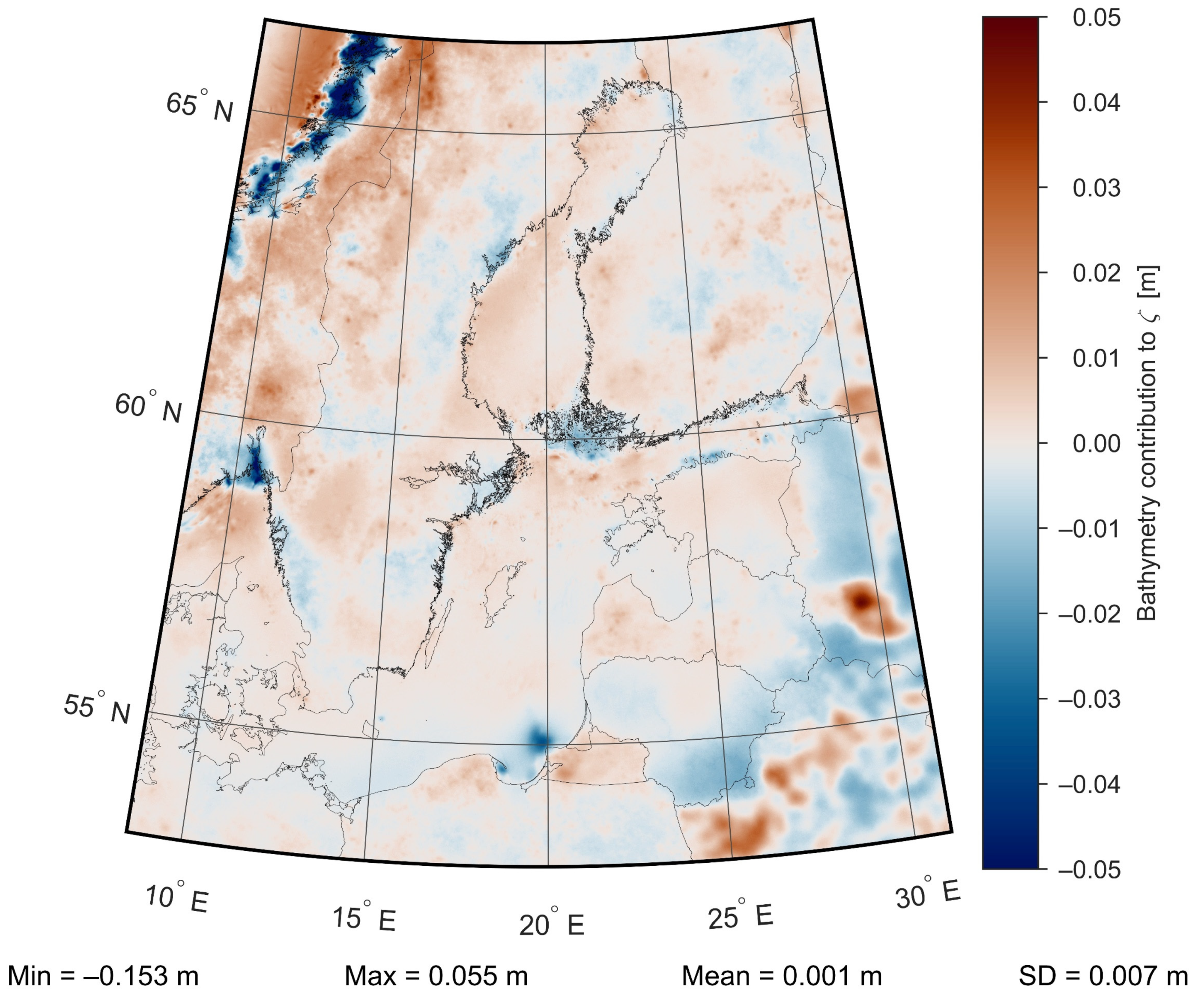
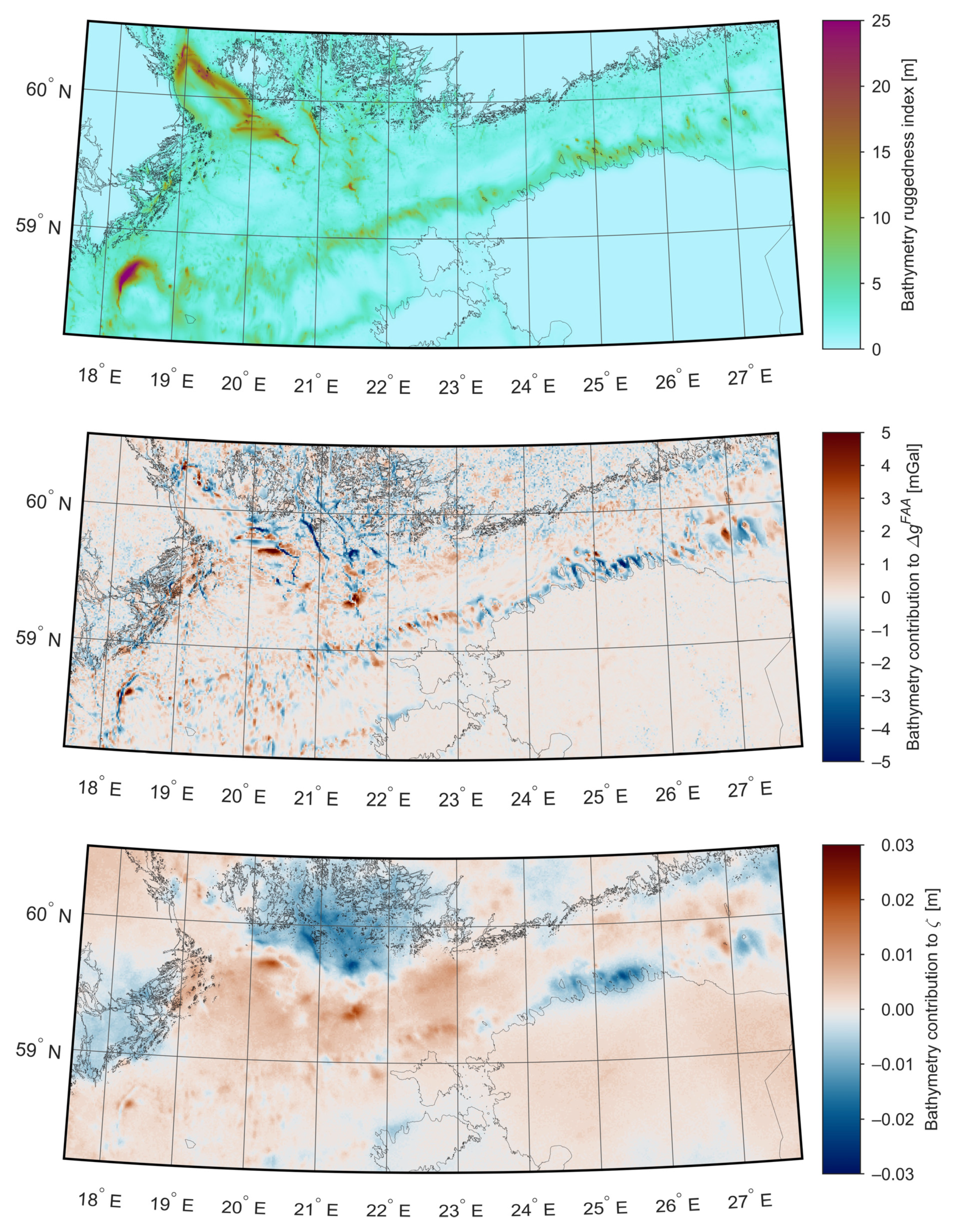
4.5. Bathymetry Influence on Geoid Modeling

Considering both the GNSS-leveling and profile-based comparisons, the GOCO05c-based regional gravimetric geoid solution, where modification limits were set to 200, seems to show good overall accuracy. The model is presented in Figure 14. Similar to the previous bathymetry influence investigations, the contribution to geoid modeling was derived by comparing the model to its counterpart, which used the surface free-air anomaly grid where bathymetry information was neglected during the computation.

Examination of geoid modeling differences (Figure 15) indicates that most variability in the Baltic Sea remains within 2 cm, being generally around a centimeter. The same magnitude differences can be noticed inland due to causes discussed in Section 4.2 and Section 4.3, which also influence geoid modeling results. More considerable area-extensive differences inland and in the southern Baltic Sea are in regions of sparse or no gravity data (refer, e.g., to Figure 8). However, in the central Baltic Sea and the Gulf of Finland, larger detailed differences up to 3–4 cm can be detected. Comparing the bathymetry ruggedness index to the bathymetry influence on the modeling results in Figure 16 shows that these differences appear in more rugged regions of the seabed. Figure 16 also shows more detailed similarities between the bathymetry ruggedness index and the bathymetry contribution to gridded surface free-air anomalies, previously mentioned in Section 4.3.

The most significant influence of bathymetry consideration can again be seen near the coastal areas of Norway, where bathymetry is most rugged (cf. Figure 3), resulting in differences around a decimeter (but can reach up to 15 cm). Although these differences in geoid features are much smoother than the computed bathymetry ruggedness index, the correlation coefficient between the two datasets is 0.65 (all marine areas in the geoid modeling target area were considered; absolute values of bathymetry contribution to geoid modeling results were used). The discussed results suggest that consideration for bathymetry has allowed the inclusion of short-wavelength details of the marine geoid in the modeling results.

To further examine the influence of bathymetry on geoid modeling, the validation results of GOCO05c-based solutions (by considering/neglecting bathymetry) with modification limits of 200 were compared. Differences between the two sets of comparisons shown in Figure 17 appear to be minor. For demonstration, Figure 18 presents comparisons of another two solutions. Since GOCO06s-based models appeared to perform well over marine areas at higher modification limits (cf. Figure 13), the respective solutions with limits of 280 were selected for presentation. By comparing Figure 17 and Figure 18, it is clear that the considering/neglecting bathymetry tendencies change. The validation differences in Figure 17 and Figure 18 are primarily caused by the long-wavelength contributions caused by GGM and modification limits’ choice and not due to the influence of bathymetry. Additionally, the contribution of bathymetry is too localized, and the accuracy of marine profiles is too low to say with certainty whether bathymetry has contributed positively or not using these validation results. An exception could be the Salme GNSS C5 profiles that largely coincide with the bathymetry-induced localized changes north of Estonia (cf. Figure 4 and Figure 16), suggesting that modeling has benefited slightly from bathymetry (cf. Figure 17 and Figure 18). On a side note, a comparison between difference plots (e.g., Figure 15 compared to GOCO06s-based solutions’ differences) would result in discrepancies of long-wavelength nature. The short-wavelength differences between modeling solutions are similar regardless of the selection of GGM and modification limits.

A more detailed look was taken at Norway, where geoid modeling differences due to bathymetry were the largest. The residual values relative to GNSS-leveling control points (Figure 19) show significant modeling improvements up to around a decimeter in locations where bathymetry contributed the most (also refer to Figure 15). Therefore, considering high-frequency gravity field variations due to bathymetry during geoid modeling (in this study, within RTM reduction) can significantly increase the resulting model accuracy, especially in regions with the rugged seabed (cf. Figure 3). Based on improvements in Norway, it could be assumed that the localized details of the marine geoid that appear due to consideration for bathymetry have similarly increased the modeling accuracy (e.g., in the central Baltic Sea).

5. Discussion

This study investigated bathymetry’s influence on gravity field estimation and geoid modeling in the Baltic Sea region in Northern Europe. By accounting for bathymetry-based RTM reduction during gravity data processing, valuable short-wavelength gravity information can be retained in the gridded gravity field (cf. Figure 11). The influence of bathymetry was especially significant in regions of rugged terrain/bathymetry (e.g., Norwegian fjords; also refer to Figure 3), where up to around 40 mGal differences (relative to neglecting bathymetry during gravity field estimation) could be observed. These gravity field refinements propagated further to the determined geoid models. The differences (relative to neglecting bathymetry) were up to 3–4 cm in some sparse regions of the Baltic Sea, being generally around a centimeter (cf. Figure 15 and Figure 16). However, a significant influence of bathymetry on geoid modeling could be seen in the coastal area of Norway, where geoid modeling accuracy improved up to around a decimeter (cf. Figure 19).

Conventionally, precise GNSS-leveling control points are employed to validate geoid modeling results. Unfortunately, such control data are limited to land areas. This study demonstrated that various marine measurements (e.g., shipborne GNSS or airborne laser scanning) could be beneficial in assessing the performance of various marine geoid modeling solutions. Figure 13 presented such a validation case with a total of 68 geoid models. Although the accuracy of geoidal heights derived from marine measurements is not comparable to GNSS-leveling control points due to dynamic measuring conditions and inaccuracies in dynamic topography estimation (required to determine geoidal heights from the measured sea surface heights), the geometric information these data provide can be invaluable.

In this study, such marine profiles were limited to a small area around Estonia and Latvia (cf. Figure 4). Only the Salme GNSS C5 profiles (north of Estonia) coincided well (considering the whole dataset) with more considerable geoid modeling differences due to bathymetry. These validation results indicated a slight modeling improvement when bathymetry was considered (cf. Figure 17 and Figure 18). In other validation cases using different datasets, differences due to GGM and modification limits’ choice dominated. In future studies, it would be interesting to investigate how satellite altimetry, which can provide sea surface heights with worldwide coverage, could benefit the validation of marine geoid models in a similar manner (also see [82]). Importantly, from a statistical point of view, altimetry measurements could also allow a more uniformly distributed dataset of points for validation.

It is essential to address that by using RTM reduction during data processing, the influence of bathymetry is not limited to marine areas but also propagates inland (cf. Figure 7). These influences can then affect subsequent gravity field estimation and geoid modeling. A good quality dataset of depth information is thus required, whereas poor bathymetry data may reduce the modeling accuracy. According to the results of this study, even the 15″ × 15″ GEBCO grid can contribute significantly to the improvement of geoid modeling solutions (cf. Figure 19), suggesting the good quality of the GEBCO bathymetry data in the Northern Europe region.

Here, the unbiased LSMSA modeling approach was employed for geoid determination, where the benefits of bathymetry consideration are introduced during gravity field estimation. The remove–compute–restore technique is another widely used geoid modeling method. In that, the terrain and GGM effects are removed from gravity data, and Stokes’s formula is applied to the residual gravity values, after which the removed effects are restored. The bathymetry information would then be used in estimating the terrain effects. It is believed that a similar influence of bathymetry to geoid modeling could be expected using that method (also see [30]).

6. Conclusions

Northern Europe has been the target area in many regionwide geoid determination studies. However, the research has been land-focused and bathymetry information has been neglected. This study demonstrated that considering bathymetry through RTM reduction in gravity field estimation could help refine the results by retaining valuable short-wavelength gravity information. These refinements can then help enhance geoid modeling accuracy, whereby significant improvements can be expected in the rugged seabed regions. The geoid modeling accuracy increased up to around a decimeter in the coastal areas of Norway, where bathymetry contributed the most. It is concluded that the inclusion of bathymetry information in computations can improve geoid modeling outcomes in future Northern Europe geoid determination projects. Although the focus was on the Baltic Sea region, it is expected that similar outcomes could be observed in other parts of the world.

References

1. Gruber, T.; Willberg, M. Signal and error assessment of GOCE-based high resolution gravity field models. J. Geod. Sci. 2019, 9, 71–86. [Google Scholar] [CrossRef]
2. Brockmann, J.M.; Schubert, T.; Schuh, W.-D. An improved model of the Earth’s static gravity field solely derived from reprocessed GOCE data. Surv. Geophys. 2021, 42, 277–316. [Google Scholar] [CrossRef]
3. Huang, J. Determining coastal mean dynamic topography by geodetic methods. Geophys. Res. Lett. 2017, 44, 11125–11128. [Google Scholar] [CrossRef]
4. Andersen, O.B.; Nielsen, K.; Knudsen, P.; Hughes, C.W.; Bingham, R.; Fenoglio-Marc, L.; Gravelle, M.; Kern, M.; Polo, S.P. Improving the coastal mean dynamic topography by geodetic combination of tide gauge and satellite altimetry. Mar. Geod. 2018, 41, 517–545. [Google Scholar] [CrossRef]
5. Idžanović, M.; Ophaug, V.; Andersen, O.B. The coastal mean dynamic topography in Norway observed by CryoSat-2 and GOCE. Geophys. Res. Lett. 2017, 44, 5609–5617. [Google Scholar] [CrossRef] [Green Version]
6. Knudsen, P.; Andersen, O.; Maximenko, N. A new ocean mean dynamic topography model, derived from a combination of gravity, altimetry and drifter velocity data. Adv. Space Res. 2021, 68, 1090–1102. [Google Scholar] [CrossRef]
7. Stokes, G.G. On the variation of gravity on the surface of the Earth. Trans. Cambridge Philos. Soc. 1849, 8, 672–695. [Google Scholar]
8. Molodenskii, M.S.; Eremeev, V.F.; Yurkina, M. Methods for Study of the External Gravitational Field and Figure of the Earth; Israel Program for Scientific Translations: Jerusalem, Israel, 1962. [Google Scholar]
9. Sjöberg, L.E.; Hunegnaw, A. Some modifications of Stokes’ formula that account for truncation and potential coefficient errors. J. Geod. 2000, 74, 232–238. [Google Scholar] [CrossRef]
10. Ellmann, A. Two deterministic and three stochastic modifications of Stokes’s formula: A case study for the Baltic countries. J. Geod. 2005, 79, 11–23. [Google Scholar] [CrossRef]
11. Goyal, R.; Ågren, J.; Featherstone, W.E.; Sjöberg, L.E.; Dikshit, O.; Balasubramanian, N. Empirical comparison between stochastic and deterministic modifiers over the French Auvergne geoid computation test-bed. Surv. Rev. 2022, 54, 57–69. [Google Scholar] [CrossRef]
12. Sjöberg, L.E. A computational scheme to model the geoid by the modified Stokes formula without gravity reductions. J. Geod. 2003, 77, 423–432. [Google Scholar] [CrossRef]
13. Sjöberg, L.E.; Bagherbandi, M. (Eds.) Applications and comparisons of LSMSA and RCR. In Gravity Inversion and Integration; Springer: Cham, Switzerland, 2017; pp. 181–202. [Google Scholar] [CrossRef]
14. Wang, Y.M.; Sánchez, L.; Ågren, J.; Huang, J.; Forsberg, R.; Abd-Elmotaal, H.A.; Ahlgren, K.; Barzaghi, R.; Bašić, T.; Carrion, D.; et al. Colorado geoid computation experiment: Overview and summary. J. Geod. 2021, 95, 127. [Google Scholar] [CrossRef]
15. Märdla, S.; Ågren, J.; Strykowski, G.; Oja, T.; Ellmann, A.; Forsberg, R.; Bilker-Koivula, M.; Omang, O.; Paršeliūnas, E.; Liepinš, I.; et al. From discrete gravity survey data to a high-resolution gravity field representation in the Nordic-Baltic region. Mar. Geod. 2017, 40, 416–453. [Google Scholar] [CrossRef]
16. Sakil, F.F.; Erol, S.; Ellmann, A.; Erol, B. Geoid modeling by the least squares modification of Hotine’s and Stokes’ formulae using non-gridded gravity data. Comput. Geosci. 2021, 156, 104909. [Google Scholar] [CrossRef]
17. dos Santos, N.P.; Escobar, I.P. Discrete evaluation of Stokes’s integral by means of Voronoi and Delaunay structures. J. Geod. 2004, 78, 354–367. [Google Scholar] [CrossRef]
18. Omang, O.C.D.; Forsberg, R. How to handle topography in practical geoid determination: Three examples. J. Geod. 2000, 74, 458–466. [Google Scholar] [CrossRef]
19. Tscherning, C.C.; Forsberg, R. Geoid determination in the Nordic countries from gravity and height data. Boll. Geod. Sci. Affin. 1987, 46, 21–43. [Google Scholar]
20. Forsberg, R. A new high-resolution geoid of the Nordic area. In Determination of the Geoid; Rapp, R.H., Sansò, F., Eds.; Springer: New York, NY, USA, 1991; pp. 241–250. [Google Scholar] [CrossRef]
21. Forsberg, R.; Kaminskis, J.; Solheim, D. Geoid of the Nordic and Baltic region from gravimetry and satellite altimetry. In Gravity, Geoid and Marine Geodesy; Segawa, J., Fujimoto, H., Okubo, S., Eds.; Springer: Berlin, Germany, 1997; pp. 540–547. [Google Scholar] [CrossRef]
22. Denker, H.; Torge, W. The European gravimetric quasigeoid EGG97—An IAG supported continental enterprise. In Geodesy on the Move; Forsberg, R., Feissel, M., Dietrich, R., Eds.; Springer: Berlin, Germany, 1998; pp. 249–254. [Google Scholar] [CrossRef]
23. Omang, O.C.D.; Forsberg, R. The Northern European geoid: A case study on long-wavelength geoid errors. J. Geod. 2002, 76, 369–380. [Google Scholar] [CrossRef]
24. Forsberg, R.; Strykowski, G.; Solheim, D. NKG-2004 geoid of the Nordic and Baltic area. In Proceedings of the International Association of Geodesy Symposium on Gravity, Geoid, and Space Missions, Porto, Portugal, 30 August–3 September 2004. [Google Scholar]
25. Denker, H.; Barriot, J.-P.; Barzaghi, R.; Fairhead, D.; Forsberg, R.; Ihde, J.; Kenyeres, A.; Marti, U.; Sarrailh, M.; Tziavos, I.N. The development of the European gravimetric geoid model EGG07. In Observing our Changing Earth; Sideris, M.G., Ed.; Springer: Berlin, Germany, 2009; pp. 177–185. [Google Scholar] [CrossRef]
26. Denker, H. Regional gravity field modeling: Theory and practical results. In Sciences of Geodesy—II.; Xu, G., Ed.; Springer: Berlin, Germany, 2013; pp. 185–291. [Google Scholar] [CrossRef] [Green Version]
27. Ågren, J.; Strykowski, G.; Bilker-Koivula, M.; Omang, O.; Märdla, S.; Oja, T.; Ellmann, A.; Liepins, I.; Parseliunas, E.; Forsberg, R.; et al. On the development of the new Nordic gravimetric geoid model NKG2015. In Proceedings of the 26th International Union of Geodesy and Geophysics General Assembly, Prague, Czech Republic, 22 June–2 July 2015. [Google Scholar] [CrossRef]
28. Denker, H. A new European gravimetric (quasi)geoid EGG2015. In Proceedings of the 26th International Union of Geodesy and Geophysics General Assembly, Prague, Czech Republic, 22 June–2 July 2015. [Google Scholar]
29. Ågren, J.; Strykowski, G.; Bilker-Koivula, M.; Omang, O.; Märdla, S.; Forsberg, R.; Ellmann, A.; Oja, T.; Liepins, I.; Parseliunas, E.; et al. The NKG2015 gravimetric geoid model for the Nordic-Baltic region. In Proceedings of the International Symposium on Gravity, Geoid and Height Systems 2016, Thessaloniki, Greece, 19–23 September 2016. [Google Scholar] [CrossRef]
30. Dahl, O.C.; Forsberg, R. Geoid models around Sognefjord using depth data. J. Geod. 1998, 72, 547–556. [Google Scholar] [CrossRef]
31. Schwabe, J.; Ågren, J.; Liebsch, G.; Westfeld, P.; Hammarklint, T.; Mononen, J.; Andersen, O.B. The Baltic Sea Chart Datum 2000 (BSCD2000)—Implementation of a common reference level in the Baltic Sea. Int. Hydrogr. Rev. 2020, 23, 63–83. [Google Scholar]
32. Varbla, S.; Ågren, J.; Ellmann, A.; Poutanen, M. Treatment of tide gauge time series and marine GNSS measurements for vertical land motion with relevance to the implementation of the Baltic Sea Chart Datum 2000. Remote Sens. 2022, 14, 920. [Google Scholar] [CrossRef]
33. Bouin, M.-N.; Ballu, V.; Calmant, S.; Boré, J.-M.; Folcher, E.; Ammann, J. A kinematic GPS methodology for sea surface map-ping, Vanuatu. J. Geod. 2009, 83, 1203. [Google Scholar] [CrossRef]
34. Saari, T.; Bilker-Koivula, M.; Koivula, H.; Nordman, M.; Häkli, P.; Lahtinen, S. Validating geoid models with marine GNSS measurements, sea surface models, and additional gravity observations in the Gulf of Finland. Mar. Geod. 2021, 44, 196–214. [Google Scholar] [CrossRef]
35. Varbla, S.; Liibusk, A.; Ellmann, A. Shipborne GNSS-determined sea surface heights using geoid model and realistic dynamic topography. Remote Sens. 2022, 14, 2368. [Google Scholar] [CrossRef]
36. Gruno, A.; Liibusk, A.; Ellmann, A.; Oja, T.; Vain, A.; Jürgenson, H. Determining sea surface heights using small footprint airborne laser scanning. In Proceedings of the Remote Sensing of the Ocean, Sea Ice, Coastal Waters, and Large Water Regions 2013, Dresden, Germany, 23–26 September 2013. [Google Scholar] [CrossRef]
37. Zlinszky, A.; Timár, G.; Weber, R.; Székely, B.; Briese, C.; Ressl, C.; Pfeifer, N. Observation of a local gravity potential isosurface by airborne lidar of Lake Balaton, Hungary. Solid Earth 2014, 5, 355–369. [Google Scholar] [CrossRef] [Green Version]
38. Varbla, S.; Ellmann, A.; Delpeche-Ellmann, N. Applications of airborne laser scanning for determining marine geoid and surface waves properties. Eur. J. Remote Sens. 2021, 54, 557–567. [Google Scholar] [CrossRef]
39. Jahanmard, V.; Delpeche-Ellmann, N.; Ellmann, A. Realistic dynamic topography through coupling geoid and hydrodynamic models of the Baltic Sea. Cont. Shelf Res. 2021, 222, 104421. [Google Scholar] [CrossRef]
40. Heiskanen, W.A.; Moritz, H. Physical Geodesy; W. H. Freeman and Company: San Francisco, CA, USA, 1967. [Google Scholar]
41. Moritz, H. Geodetic Reference System 1980. J. Geod. 2000, 74, 128–133. [Google Scholar] [CrossRef]
42. Forsberg, R.; Tscherning, C.C. The use of height data in gravity field approximation by collocation. J. Geophys. Res. Solid Earth 1981, 86, 7843–7854. [Google Scholar] [CrossRef]
43. Forsberg, R. A Study of Terrain Reductions, Density Anomalies and Geophysical Inversion Methods in Gravity Field Modelling; Ohio State University: Columbus, OH, USA, 1984. [Google Scholar]
44. Moritz, H. Advanced Physical Geodesy; Wichmann: Karlsruhe, Germany, 1980. [Google Scholar]
45. Kasper, J.F. A second-order Markov gravity anomaly model. J. Geophys. Res. 1971, 76, 7844–7849. [Google Scholar] [CrossRef]
46. Sjöberg, L.E. Refined least squares modification of Stokes’ formula. Manus. Geod. 1991, 16, 367–375. [Google Scholar]
47. Ellmann, A. Computation of three stochastic modifications of Stokes’s formula for regional geoid determination. Comput. Geosci. 2005, 31, 742–755. [Google Scholar] [CrossRef]
48. Ellmann, A. Using high-resolution spectral models of gravity anomaly for computing stochastic modifications of Stokes’s formula. Comput. Geosci. 2012, 39, 188–190. [Google Scholar] [CrossRef]
49. Paul, M.K. A method of evaluating the truncation error coefficients for geoidal height. Bull. Géodésique 1973, 110, 413–425. [Google Scholar] [CrossRef]
50. Hagiwara, Y. A new formula for evaluating the truncation error coefficient. Bull. Géodésique 1976, 50, 131–135. [Google Scholar] [CrossRef]
51. Sjöberg, L.E. A solution to the downward continuation effect on the geoid determined by Stokes’ formula. J. Geod. 2003, 77, 94–100. [Google Scholar] [CrossRef]
52. Sjöberg, L.E. The IAG approach to the atmospheric geoid correction in Stokes’ formula and a new strategy. J. Geod. 1999, 73, 362–366. [Google Scholar] [CrossRef]
53. Sjöberg, L.E.; Nahavandchi, H. The atmospheric geoid effects in Stokes’ formula. Geophys. J. Int. 2000, 140, 95–100. [Google Scholar] [CrossRef] [Green Version]
54. Sjöberg, L.E. Topographic and atmospheric corrections of gravimetric geoid determination with special emphasis on the effects of harmonics of degrees zero and one. J. Geod. 2001, 75, 283–290. [Google Scholar] [CrossRef]
55. Sjöberg, L.E. Ellipsoidal corrections to order e2 of geopotential coefficients and Stokes’ formula. J. Geod. 2003, 77, 139–147. [Google Scholar] [CrossRef]
56. Ellmann, A.; Sjöberg, L.E. Ellipsoidal correction for the modified Stokes formula. Boll. Geod. Sci. Affin. 2004, 63, 153–172. [Google Scholar]
57. Sjöberg, L.E. A spherical harmonic representation of the ellipsoidal correction to the modified Stokes formula. J. Geod. 2004, 78, 180–186. [Google Scholar] [CrossRef]
58. Ågren, J.; Sjöberg, L.E.; Kiamehr, R. The new gravimetric quasigeoid model KTH08 over Sweden. J. Appl. Geod. 2009, 3, 143–153. [Google Scholar] [CrossRef]
59. Ellmann, A. A numerical comparison of different ellipsoidal corrections to Stokes’ formula. In A Window on the Future of Geodesy; Sansò, F., Ed.; Springer: Berlin, Germany, 2005; pp. 409–414. [Google Scholar] [CrossRef]
60. Märdla, S.; Ellmann, A.; Ågren, J.; Sjöberg, L.E. Regional geoid computation by least squares modified Hotine’s formula with additive corrections. J. Geod. 2018, 92, 253–270. [Google Scholar] [CrossRef]
61. Ekman, M. Impacts of geodynamic phenomena on systems for height and gravity. Bull. Géodésique 1989, 63, 281–296. [Google Scholar] [CrossRef]
62. Poutanen, M.; Vermeer, M.; Mäkinen, J. The permanent tide in GPS positioning. J. Geod. 1996, 70, 499–504. [Google Scholar] [CrossRef]
63. GEBCO_2021 Grid. Available online: https://doi.org/10.5285/c6612cbe-50b3-0cff-e053-6c86abc09f8f (accessed on 25 March 2022).
64. Hao, R.; Wan, X.; Wang, Y.; Annan, R.F.; Sui, X. Evaluation of four global bathymetry models by shipborne depths data. J. Surv. Eng. 2022, 148, 04021033. [Google Scholar] [CrossRef]
65. Leppäranta, M.; Myrberg, K. Physical Oceanography of the Baltic Sea; Springer: Berlin, Germany, 2009. [Google Scholar] [CrossRef]
66. Riley, S.J.; DeGloria, S.D.; Elliot, R. A terrain ruggedness index that quantifies topographic heterogeneity. Intermt. J. Sci. 1999, 5, 23–27. [Google Scholar]
67. Pail, R.; Gruber, T.; Fecher, T.; GOCO Project Team. The combined gravity model GOCO05c. GFZ Data Serv. 2016. [Google Scholar] [CrossRef]
68. Fecher, T.; Pail, R.; Gruber, T.; the GOCO Consortium. GOCO05c: A new combined gravity field model based on full normal equations and regionally varying weighting. Surv. Geophys. 2017, 38, 571–590. [Google Scholar] [CrossRef]
69. Förste, C.; Abrykosov, O.; Bruinsma, S.; Dahle, C.; König, R.; Lemoine, J.-M. ESA’s release 6 GOCE gravity field model by means of the direct approach based on improved filtering of the reprocessed gradients of the entire mission (GO_CONS_GCF_2_DIR_R6). GFZ Data Serv. 2019. [Google Scholar] [CrossRef]
70. Kvas, A.; Mayer-Gürr, T.; Krauss, S.; Brockmann, J.M.; Schubert, T.; Schuh, W.-D.; Pail, R.; Gruber, T.; Jäggi, A.; Meyer, U. The satellite-only gravity field model GOCO06s. GFZ Data Serv. 2019. [Google Scholar] [CrossRef]
71. Kvas, A.; Brockmann, J.M.; Krauss, S.; Schubert, T.; Gruber, T.; Meyer, U.; Mayer-Gürr, T.; Schuh, W.-D.; Jäggi, A.; Pail, R. GOCO06s—A satellite-only global gravity field model. Earth Syst. Sci. Data 2021, 13, 99–118. [Google Scholar] [CrossRef]
72. Zingerle, P.; Pail, R.; Gruber, T.; Oikonomidou, X. The experimental gravity field model XGM2019e. GFZ Data Serv. 2019. [Google Scholar] [CrossRef]
73. Zingerle, P.; Pail, R.; Gruber, T.; Oikonomidou, X. The combined global gravity field model XGM2019e. J. Geod. 2020, 94, 66. [Google Scholar] [CrossRef]
74. Rüdja, A.; Varbla, S. Estonian GNSS-leveling dataset with relevance to the implementation of the Baltic Sea Chart Datum 2000. SEANOE 2022. [Google Scholar] [CrossRef]
75. Vestøl, O.; Ågren, J.; Steffen, H.; Kierulf, H.; Tarasov, L. NKG2016LU: A new land uplift model for Fennoscandia and the Baltic region. J. Geod. 2019, 93, 1759–1779. [Google Scholar] [CrossRef] [Green Version]
76. Varbla, S.; Ellmann, A.; Delpeche-Ellmann, N. Validation of marine geoid models by utilizing hydrodynamic model and shipborne GNSS profiles. Mar. Geod. 2020, 43, 134–162. [Google Scholar] [CrossRef]
77. Liibusk, A.; Varbla, S.; Ellmann, A.; Vahter, K.; Uiboupin, R.; Delpeche-Ellmann, N. Shipborne GNSS acquisition of sea surface heights in the Baltic Sea. J. Geod. Sci. 2022. in print. [Google Scholar] [CrossRef]
78. Forsberg, R.; Olesen, A.V.; Keller, K.; Møller, M.; Gidskehaug, A.; Solheim, D. Airborne gravity and geoid surveys in the Arctic and Baltic seas. In Proceedings of the International Symposium on Kinematic Systems in Geodesy, Geomatics and Navigation (KIS-2001), Banff, Canada, 5–8 June 2001. [Google Scholar]
79. Ellmann, A. Downward continuation of airborne gravity data using high-resolution global geopotential models. In Proceedings of the 8th International Conference on Environmental Engineering, Vilnius, Lithuania, 19–20 May 2011. [Google Scholar]
80. Förste, C.; Bruinsma, S.L.; Abrykosov, O.; Lemoine, J.-M.; Marty, J.C.; Flechtner, F.; Balmino, G.; Barthelmes, F.; Biancale, R. EIGEN-6C4 the latest combined global gravity field model including GOCE data up to degree and order 2190 of GFZ Potsdam and GRGS Toulouse. GFZ Data Serv. 2014. [Google Scholar] [CrossRef]
81. Oja, T.; Ellmann, A.; Märdla, S. Gravity anomaly field over Estonia. Estonian J. Earth Sci. 2019, 68, 55–75. [Google Scholar] [CrossRef]
82. Mostafavi, M.; Delpeche-Ellmann, N.; Ellmann, A. Accurate sea surface heights from Sentinel-3A and Jason-3 retrackers by incorporating high-resolution marine geoid and hydrodynamic models. J. Geod. Sci. 2021, 11, 58–74. [Google Scholar] [CrossRef]
Figure 1. Terrain elevations and bathymetry. The dashed blue line surrounding Estonia shows the boundaries of the Estonian Maritime Administration obtained bathymetry data. Red dots are GNSS-leveling control point locations, and the green rectangle denotes the geoid modeling target area.
Jmse 10 00793 g001
Figure 2. Surface free-air anomalies (final release of BSCD2000 dataset version 3).
Jmse 10 00793 g002
Figure 3. Estimated ruggedness of bathymetry.
Jmse 10 00793 g003
Figure 4. Shipborne GNSS-determined and airborne laser scanning-derived marine profiles of geoidal heights.
Jmse 10 00793 g004
Figure 5. A priori error estimates of gravity data.
Jmse 10 00793 g005
Figure 6. RTM reduction computed by also considering bathymetry information.
Jmse 10 00793 g006
Figure 7. Bathymetry contribution to RTM reduction.
Jmse 10 00793 g007
Figure 8. RTM anomalies computed by also considering bathymetry information.
Jmse 10 00793 g008
Figure 9. Empirical autocovariance curves and respective least-squares fitted second-order Markov covariance models with the associated correlation lengths X 1 / 2 (shown with dashed lines) and signal variances C0 (see the legend).
Jmse 10 00793 g009
Figure 10. Gridded surface free-air anomalies computed by also considering bathymetry information.
Jmse 10 00793 g010
Figure 11. Bathymetry contribution to gridded surface free-air anomalies.
Jmse 10 00793 g011
Figure 12. Validation results of gravimetric geoid models using GNSS-leveling control points.
Jmse 10 00793 g012
Figure 13. Validation results of gravimetric geoid models using shipborne GNSS-determined and airborne laser scanning-derived marine profiles of geoidal heights.
Jmse 10 00793 g013
Figure 14. Gravimetric geoid modeling solution of the Baltic Sea region. GGM: GOCO05c, modification limits: 200, bathymetry was considered in computations.
Jmse 10 00793 g014
Figure 15. Bathymetry contribution to geoid modeling results. GGM: GOCO05c, modification limits: 200.
Jmse 10 00793 g015
Figure 16. Estimated ruggedness of bathymetry (up), bathymetry contribution to gridded surface free-air anomalies (middle) and bathymetry contribution to geoid modeling results (down; GGM: GOCO05c, modification limits: 200) in the central Baltic Sea and the Gulf of Finland.
Jmse 10 00793 g016
Figure 17. Validation results of gravimetric geoid models. GGM: GOCO05c, modification limits: 200.
Jmse 10 00793 g017
Figure 18. Validation results of gravimetric geoid models. GGM: GOCO06s, modification limits: 280.
Jmse 10 00793 g018
Figure 19. Residuals (mean removed) of gravimetric geoid models relative to the Norwegian GNSS-leveling control points. GGM: GOCO05c, modification limits: 200. The sizes of colored dots are proportional to the residual values.
Jmse 10 00793 g019
Publisher’s Note: MDPI stays neutral with regard to jurisdictional claims in published maps and institutional affiliations.