The Motion and Deformation of Viscoplastic Slide while Entering a Body of Water

Abstract

Landslide-generated waves are hazards that, commonly, exist in the natural world. The motion and deformation of a submerged landslide significantly affect the efficiency of the momentum transfer, between the slide material and the water body, and, thereby, dominate the characteristics of the associated waves. Therefore, investigating how the submerged sliding mass is moved and deformed is of great importance, not only for understanding the physical mechanism behind the slide–water interaction but also for optimizing the predictive models of the wave characteristics. In this study, we assumed the landslide as a viscoplastic fluid and used an ideal viscoplastic material, called Carbopol, to mimic a natural landslide, at the laboratory scale. We, first, determined the coordinates of three control points, including the frontal point, deepest point, and center of mass, so as to quantify the time evolution of the submerged slide motion. We, then, fit the maximums of the coordinates of the control points with an integrated parameter of the incoming landslide, with the support of experimental data. Results indicated that not only the wave features but also the submerged slide motion can be quantified by the slide parameters on impact.

1. Introduction

One of the recent problems to be examined in the field of coastal engineering is related to the impulse waves caused by a landslide entering a water basin, such as a sea, fjord, or lake, and generating destructive waves. The largest historical event occurred at the Vajont Reservoir in Italy, in 1963: a large landslide formed an impulse wave that over-topped the dam and destroyed two villages downstream of the reservoir, causing more than 2000 deaths [1,2,3]. A more recent example was a rapid rock avalanche that occurred in 2017, in Greenland, where approximately 50 × 10 m${}^3$ of slide material impacted the Karrat Fjord and created a wave that traveled 32 km to the village of Nuugaatsiaq [4,5]. These events resulted in devastating consequences for the coastal areas, which motivated researchers to discover the physics behind the events and to build predictive models to assess and evaluate any potential hazards.

Researchers have developed a series of empirical equations to express unknown wave characteristics, such as the maximum wave height, amplitude, and period, as functions of slide features, such as slide thickness, mass, and velocity [6,7,8,9,10]. Efforts, also, have been taken, to understand the physical mechanisms governing the impact process [11,12]. Zitti et al. (2016) developed a theoretical model to describe the momentum transfer between the sliding mass and the body of water [13]. They simplified the slide–water interaction, by assuming each particle enters the body of water, independently, and expressed the interaction force between the immersed slide and the body of water, using a simple linear equation. However, in the real world, the interaction force could be affected by many factors, which are not contained in the simplified equation, for example, the motion and deformation of the submerged sliding mass. Fush et al. (2013) provided insights into the underwater slide dynamics and their final deposition patterns [14]. Zitti et al. (2017) discussed the motion of submerged granular slides, by tracing the motion of the frontal, deepest, and center points of the slide’s immersed part [15]. Yavari-Ramshe et al. (2019) indicated that the slide’s deformability may affect the characteristics of the generated waves [16]. Therefore, it is necessary to study how the submerged slide’s motion and deformation are related to the slide–water interaction and wave generation.

As most historical events were caused by granular-like landslides, researchers, often, modeled a landslide with granular models and used granular particles to mimic natural landslides in experiments [17,18]. However, a problem, suffered by experiments conducted with granular particles, was that they dispersed, quickly, to numerous individuals, and generated a huge amount of air bubbles, once they entered the body of water, which made it difficult to extract the slide–water interface from the recorded images. See Figure 1 for the spread of granular particles and generation of air bubbles.

In addition to granular models, many natural landslides can, also, be well described by viscoplastic models [19]. Viscoplastic models explain the behavior of many natural bulk materials that behave like solids, when they are at rest, and flow like fluids, under some circumstances. Laboratory experiments have demonstrated the possibilities of modeling the rheology of natural landslides, such as debris flow, clay, mud flow, and snow avalanche, by viscoplastic models [20,21]. Our recent studies, also, have modeled a landslide as a viscoplastic fluid and introduced a viscoplastic material, called Carbopol ultrez 10 to experimental studies of landslide-generated waves [22,23,24]. Carbopol is considered as one of the best-suited materials for the Herschel–Bulkley model. In recent years, Carbopol has been, increasingly, used to mimic cohesive landslides over a wide range of shear rates, in various studies, such as standard rheological measurements, channel configurations, etc. [19,25,26]. Compared with granular slides, viscoplastic materials have high cohesion and, usually, move as a whole, which make it possible to obtain a sharply marginated slide–water interface from experimental observations.

The objective of this study was to determine the motion and deformation of the sliding mass, after it entered the body of water, on the basis of physical model experiments. We considered a landslide as a viscoplastic fluid and used a viscoplastic material, called Carbopol, to mimic natural landslides. By analyzing the interaction forces between the sliding mass and the body of water, we selected three control points to evaluate the slide–water interaction: the frontal point, the deepest point, and the center of mass [15]. The center of mass was selected as an indicator of the space-averaged motion of the submerged slide. The frontal and deepest points were used to represent how the slide is stretched in water. We, then, quantified the maximum coordinates of these control points, from an integrated parameter of the slide features on impact.

2. Experimental Method

2.1. Experimental Facilities

The impacting process of landslide-generated waves can be divided into two stages: in the first stage, the slide starts to move along the chute towards the shoreline; in the second stage, it enters the body of water and generates impulse waves. Figure 2 displays the sketch of the physical process, in which the solid lines denote the first stage, and the dash lines denote the second stage.

Figure 3a,b illustrate the sketch and photo of the experimental facilities, respectively. Experiments were conducted in a two-dimensional flume, which includes two parts. The first part was a 1.5 m long and 0.12 m wide chute, with side walls made of PVC. The second part was a 2.5 m long, 0.4 m deep, and 0.12 m wide transparent glass flume. The bottom of the slope was lined with sandpaper, with a mean surface roughness that was fixed at 27.28 $\mathsf{\mu }$m. The slide material was, initially, contained in a box, located at the entrance of the slope and closed by a locked gate. Once the gate was released, the material accelerated under gravity and could reach velocities as high as 2.5 m/s. In our experiments, the initial still-water depth $h_0$ was fixed to 0.2 m, the slope angle to $\theta ={45}^{\circ }$, the slope length ${\ell }_s$ ranged between 0.65 m and 1.05 m, and the initial slide mass $m_I$ ranged between 2.0 kg and 6.0 kg, which allows the slide material to enter the water body with a wide range of slide thickness, mass, and velocity. See

Table 1. The initial settings of all the experiments.

${\mathit{l}}_{\mathit{s}}$ [m]	${\mathit{m}}_{\mathit{I}}$ [kg]
1.05	2.75, 3.0, 3.25, 3.5, 3.75, 4.0, 4.25, 4.5, 4.75, 5.0, 5.25, 5.5, 5.75, 6.0
0.95	2.75, 3.0, 3.25, 3.5, 3.75, 4.0, 4.25, 4.5, 4.75, 5.0, 5.25, 5.5, 5.75, 6.0
0.85	2.5, 2.75, 3.0, 3.25, 3.5, 3.75, 4.0,4.25, 4.5, 4.75, 5.0, 5.25, 5.5, 5.75
0.75	2.25, 2.5, 2.75, 3.0, 3.25, 3.5, 3.75, 4.0, 4.25, 4.5, 4.75, 5.0, 5.25, 5.5
0.65	2.0, 2.25, 2.5, 2.75, 3.0, 3.25, 3.5, 3.75, 4.0, 4.25, 4.5, 4.75, 5.0, 5.25

, for the initial settings of ${\ell }_s$ and $m_I$ for all experiments.

2.2. Slide Material

As for the slide material, we used a viscoplastic gel called Carbopol Ultrez 10 with a rheological behavior that depends on its concentration, which can be described by the Herschel–Bulkley equation [26,27]:

$$\tau ={\tau }_c+\mu {\dot{\gamma }}^n$$

(1)

where $\tau$ denotes the shear stress, ${\tau }_c$ is the yield stress, $\dot{\gamma }$ is the shear rate, $\mu$ is the consistency, and n is a power-law index that reflects shear thinning (or shear thickening, for $n>1$). In the present study, we used Carbopol, with a concentration c of 2.0 %. The relevant rheological parameters in Equation (1) were determined from the rheological measurements using, a Bohlin Gemini rheometer: ${\tau }_c$ = 58 Pa, K = 18.9 Pa · s${}^{-n}$, and n = 0.330. The density of Carbopol is about 1000 kg/m${}^3$, which is lower than most natural landslides (>1500 kg/m${}^3$) but similar to that of snow or ice avalanches (900 kg/m${}^3$). Details and limitations of the material, including the scale effect and density effect, refer to our earlier publications [22,23].

Compared with granular slides and rigid blocks, viscoplastic material was not only deformable but also cohesive. When it moved along the slope, part of the slide material was deposited along the chute. Consequently, it was more convenient to use the immersed part’s mass, rather than the initial mass $m_I$, to represent the slide mass m in the data analysis. We defined the immersed part’s mass, when the wave height reached its maximum, as effective mass $m_E$ [22].

Experiments were recorded using a color high-speed camera, with a resolution of 600 × 800 and a frequency of 400 fps. A 0.2 m × 0.4 m mesh grid was used to calibrate the images recorded by the camera and to determine the size-conversion factor. Figure 4 displays a series of raw images recorded from an experiment, with initial slide mass $m_I$ = 0.35 kg and slope length ${\ell }_s$ = 0.85 m. Raw images were processed using Matlab, to extract the slide–water interface and the center of mass.

3. Experimental Results

3.1. Definition of the Control Points

The principle physical mechanism governing the slide–water interaction and wave generation was the transfer of momentum, from the sliding mass to the body of water. The efficiency of the momentum transfer mainly depends on the interaction forces between the two phases, which include the hydrostastic force F${}_{\mathrm{P}}$ and the drag force F${}_{\mathrm{D}}$. In addition, as the density of the slide material selected in the present study was close to that of water, the buoyancy force was, approximately, balanced with the gravity. In this case, once the slide material entered the water body, the friction between the material and the slope bottom would be neglected, as it was small. Moreover, the material would not reach the bottom of the water basin quickly. The effect of seabed pressure was, also, neglectable.

Both the hydrostastic force and the drag force depend on the motion and deformation of the submerged sliding mass. For the viscoplastic material–water interaction, the drag force F${}_{\mathrm{D}}$ can be simplified as:

$${\mathbf{F}}_{\mathrm{D}}={\displaystyle \frac{1}{2}}{C}_d{\rho }_f{A}_f({\overline{\mathbf{u}}}_s-{\overline{\mathbf{u}}}_f)\left|{\overline{\mathbf{u}}}_s-{\overline{\mathbf{u}}}_f\right|$$

(2)

where $C_d$ is the coefficient of drag, ${\rho }_f$ is the water density, $A_f$ is the cross section area of the submerged sliding mass, ${\overline{\mathbf{u}}}_s$ is the mean velocity of the submerged slide, and ${\overline{\mathbf{u}}}_f$ is the mean velocity of the moving body of water. For the calculation of F${}_{\mathrm{D}}$, Equation (2) considered the sliding mass as a whole and simplified the slide’s velocity via its mean velocity. However, the deformation of the submerged sliding mass increases the complexity of the internal dynamics of the moving slide, which increases the difficulty of quantifying the drag force.

The hydrostastic force F${}_{\mathrm{P}}$ is a result of the change in hydrostatic pressure on the wetted surface of the sliding mass, as it enters the body of water. It can be expressed as an integration from:

$${\mathbf{F}}_{\mathrm{P}}={\int }_{A_s}-{\rho }_{f}g{h}_{sf}\mathbf{n}d{A}_s$$

(3)

where g is the gravity acceleration, $h_{sf}$ is the distance between the water surface and the slide–water interface, $\mathbf{n}$ is a vector normal to the slide–water interface, and $A_s$ is the area of the slide–water interface.

From Equations (2) to (3), we can see that the hydrostastic force F${}_{\mathrm{P}}$ and the drag force F${}_{\mathrm{D}}$ are dominated by the cross-section area of the sliding mass $A_f$, the distance between the water surface and the slide–water interface $h_{sf}$, and the area of the slide–water interface $A_s$. All these parameters are related to the evolution of the slide–water interface and the moving trajectory of the sliding mass. It means that the submerged slide motion dominates the efficiency of the momentum transfer, from the slide material to the water body, and, accordingly, affects the characteristics of the associated waves.

To simplify the submerged slide’s moving and deforming process, we analyzed the evolution of the slide–water interface in two aspects, including the submerged slide’s space-averaged motion and its overall spread. We selected three control points to represent the influencing parameters $A_f$, $A_s$, and $h_{sf}$ of the momentum transfer process, which have been mentioned above: the center of mass $(c_x,c_y)$, the frontal point ($d_x,d_y$), and the deepest point $(l_x,l_y)$. 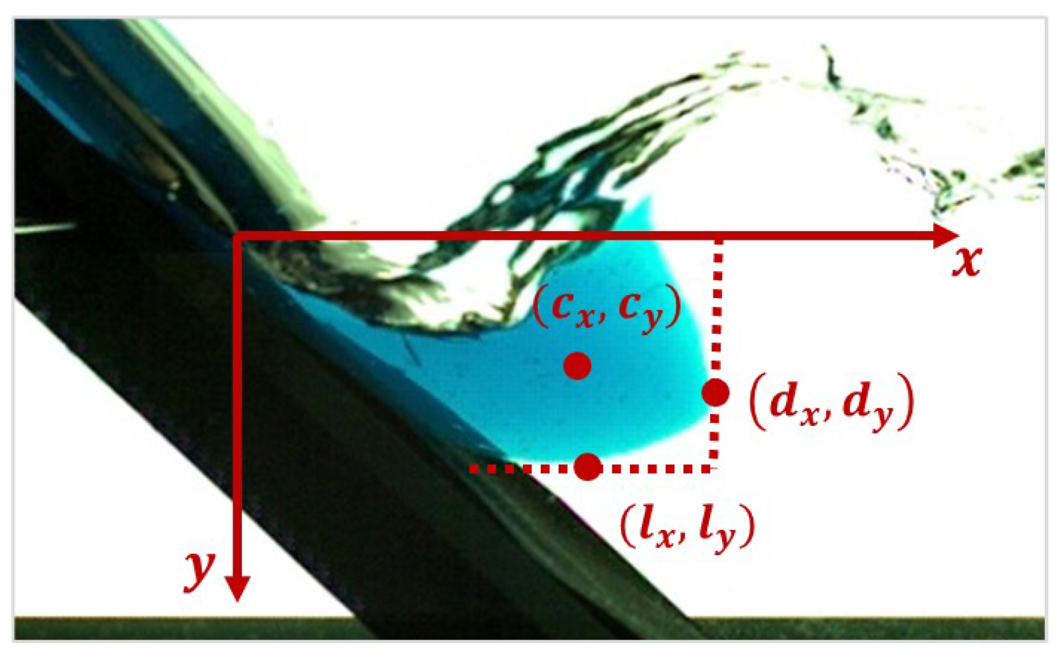Figure 5 illustrates the position of the selected control points. The deepest point of the submerged sliding mass $(l_x,l_y)$ was defined as the lowest point from the free water surface, in a vertical direction. The frontal point ($d_x,d_y$) was the farmost point away from the shoreline, in a horizontal direction. The center of mass $(c_x,c_y)$ was selected as an indicator of the space-averaged motion of the submerged sliding mass. The vertical coordinate of the deepest point $l_y$ and the horizontal coordinate of the frontal point $d_x$ were considered as the proxy of the overall motion of the submerged slide.

3.2. Motion of the Control Points

We, first, selected four representative experiments to examine the overall evolution of the center of mass of the submerged sliding mass. For each experiment, the slope angle $\theta$ = 45${}^{\circ }$ and the still-water depth $h_0$ = 0.2 m. The features of the incoming slide material were controlled by varying the initial mass of the material in the container box $m_I$ and the slope length $l_s$. See

Table 2. The initial parameters of the four selected tests.

Test Number	${\mathit{l}}_{\mathit{s}}$ [m]	${\mathit{m}}_{\mathit{I}}$ [kg]
Test 32	1.05	3.0
Test 40	0.95	3.5
Test 42	0.85	4.0
Test 46	0.85	4.5

for the $m_I$ and $l_s$ of the selected four tests.

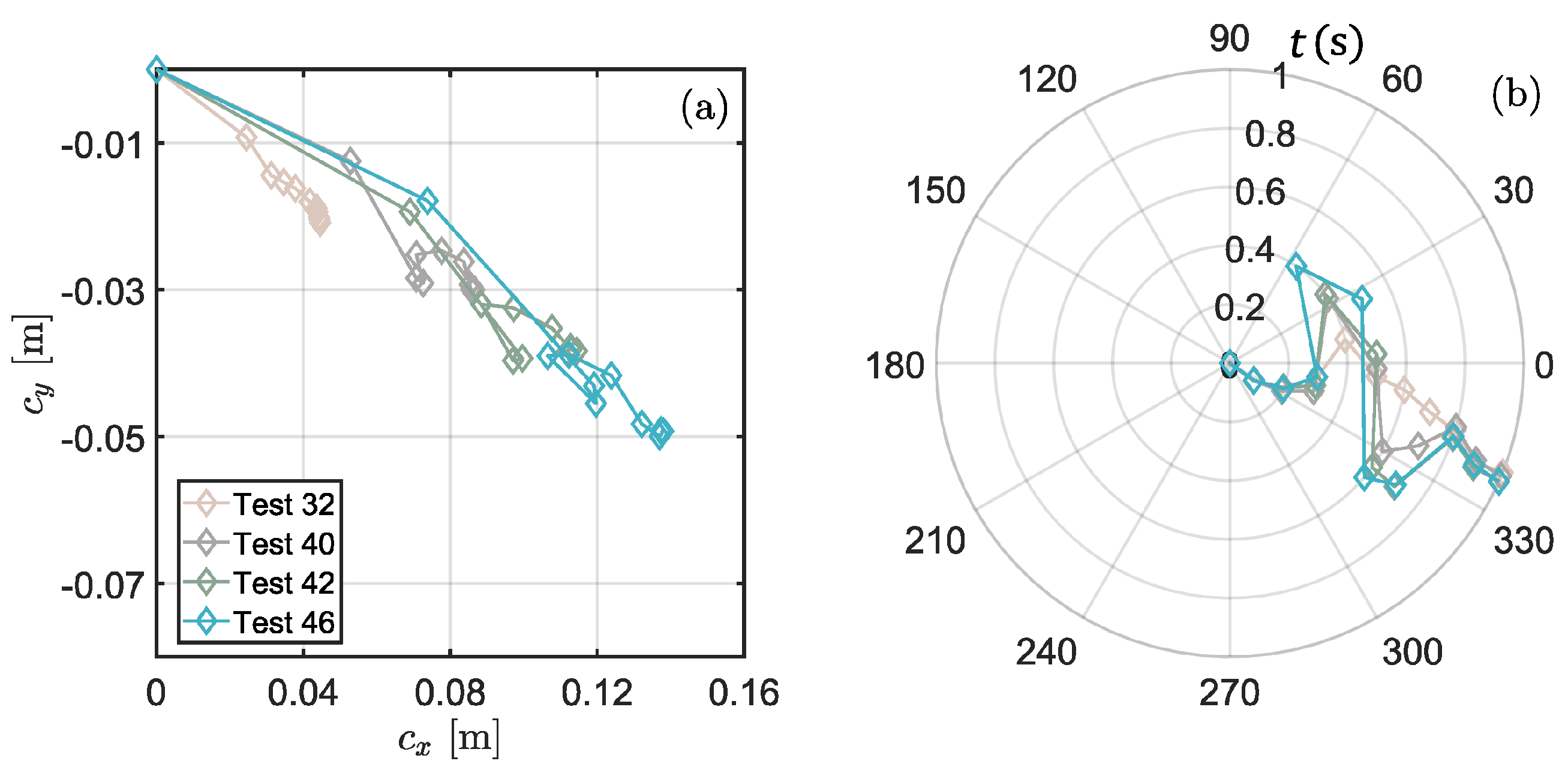
Figure 6a illustrates the time evolution of the coordinates of the center of mass ($c_x,c_y$), for the four selected experiments. It can be seen from the figure that the center of mass for all these four experiments, first, moved forward, after it crossed the shoreline, and, then, it turned back, due to the affect of the water pressure. Figure 6b displays the mean velocity of the submerged slide ${\overline{\mathbf{u}}}_s$, which provides a perspicuous view of how the submerged slide’s moving direction was turned. For these four selected experiments, both the center of mass and the mean velocity have similar trends in evolution, which means the submerged slide with different initial parameters suffered a similar deforming process.

As shown in Figure 5, the frontal point ($d_x$, $d_y$) was defined as representing the distance from the front of the sliding mass to the shoreline. The horizontal coordinate $d_x$ could, fully, represent the distance between the front boundary and the shoreline, thus, we think analyzing the evolution of $d_y$ was not necessary. Similarly, ($l_x$, $l_y$) was defined for describing the distance between the free water surface and the deepest point of the submerged sliding mass. $l_y$ could, fully, represent this information, thus, $l_x$ can be neglected in the following analysis. We, then, quantified the time evolution of the selected coordinates, i.e., $d_x\left(t\right)$, $l_y\left(t\right)$, $c_x\left(t\right)$, and $c_y\left(t\right)$.

The selected coordinates of control points were scaled by the still-water depth $h_0$: the scaled horizontal coordinate of the center of mass $C_x=c_x/h_0$, the scaled vertical coordinate of the center of mass $C_y=c_y/h_0$, the scaled horizontal coordinate of the frontal point $D_x=D_x/h_0$, and the scaled vertical coordinate of the deepest point $L_y=l_y/h_0$. Time t was scaled as $T=t{(g/h_0)}^{1/2}$. We used the impulse parameter P, proposed by Heller and Hager (2010), to represent the characteristics of the incoming landslides, with an expression that can be written as [7,9]:

$$\mathrm{P}=\mathrm{Fr}{S}^{1/2}{M}^{1/4}cos{(6/7\theta )}^{1/2}$$

(4)

where Fr = $v_0/\sqrt{g{h}_0}$ is the slide Froude number, $S=s/h_0$ is the scaled slide thickness, $M=m_E/\left({\rho }_{w}b{h}_0^2\right)$ is the scaled slide mass, $\theta$ is the slope angle, $v_0$ is the velocity at impact, s is the slide thickness, ${\rho }_w$ is the water density, $m_E$ is the effective slide mass, and b is the flume width. By varying the slope length ${\ell }_s$ and initial slide mass $m_I$, the scaled slide parameters ranged as follows: the slide Froude number is $0.05<\mathrm{Fr}<2.78$, the scaled slide mass is $0.46<M<1.23$, the scaled slide thickness is $0.12<S<0.28$, and the impulse product parameter P is $0<\mathrm{P}<1$.

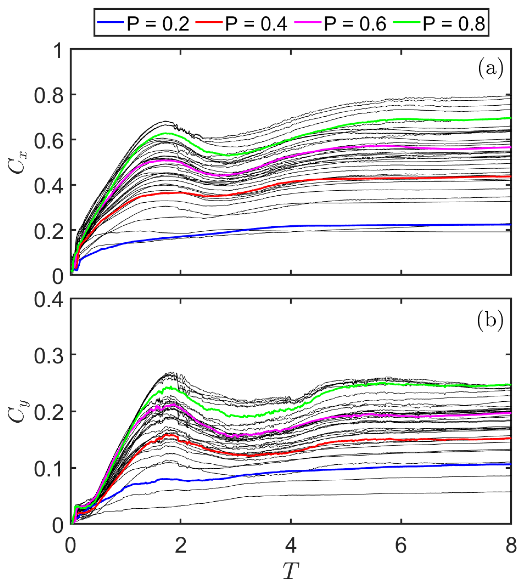
Figure 7 displays the time variation of the scaled coordinates of the center of mass $C_x\left(T\right)$ and $C_y\left(T\right)$, for experiments with different impulse product parameter P. First, as the slope angle was fixed to 45${}^{\circ }$, $C_x$ was equaled to $C_y$, for non-deformable slide materials. In our experiments, $C_x\left(T\right)$ was, generally, larger than $C_y\left(T\right)$. It means that the slide deformed upward, after it entered the water body. For most experiments, both $C_x$ and $C_y$ increased sharply at $T<2$, and, then, had a slight fluctuation at $2<T<4$. They, then, increased with a declining rate of increase at $4<T<6$, and, finally, trended to be flattened at $T>6$. It means that the center of mass in most experiments moved upward and bent to the direction of shoreline at $2<T<4$. The submerged sliding mass started to stop, since $T=4$, and, finally, stopped after $T=6$. As the impulse product parameter P could, generally, reflect the features of the incoming landslide, we examined the effects of P on the evolution of $C_x\left(T\right)$ and $C_y\left(T\right)$. In general, $C_x$ ranged within 0.2 to 0.8, and $C_y$ ranged between 0.05 and 0.25, for experiments with 0 < P < 1. Four experiments with P = 0.2, P = 0.4, P = 0.6, and P = 0.8 were emphasized in the figure. It can be seen that the impulse product parameter P greatly affects the moving trajectory of the center of mass. Experiments with larger P, usually, had larger values of $C_x\left(T\right)$ and $C_y\left(T\right)$. In addition, the fluctuation of $C_x$ and $C_y$, during $2<T<4$, was more significant for experiments with larger P, which means slides with a larger initial momentum received more water pressure and suffered a more significant deformation than slides with a lower initial momentum.

Figure 8a displays the time variation of the scaled horizontal coordinate of the frontal point $D_x\left(T\right)$, for experiments with varying P. The $D_x$ increased, with a declining rate of increase at $0<T<2$, and it trends to flatten at $T>2$. It ranged within $0<D_x<1.2$, during the whole process. In addition, similar to $C_x$ and $C_y$, the general variation of $D_x$ depended on P. Experiments with larger P led to larger values of $D_x$, on the whole. Figure 8b indicates the time variation of the scaled vertical coordinate of the deepest point $L_y\left(T\right)$, for experiments with varying P. Similar with other control points, the deepest point, also, had an obvious time node (i.e., T = 2), for all experiments, which divided the whole process into two phases, i.e., $0<T<2$ and $T>2$. $L_y\left(T\right)$ increased, quickly, with a declining rate of increase at $0<T<2$, and it trends to flatten at $T>2$. In addition, $L_y$ increases with the increase in P, with a maximum value of 0.6 in our experiments.

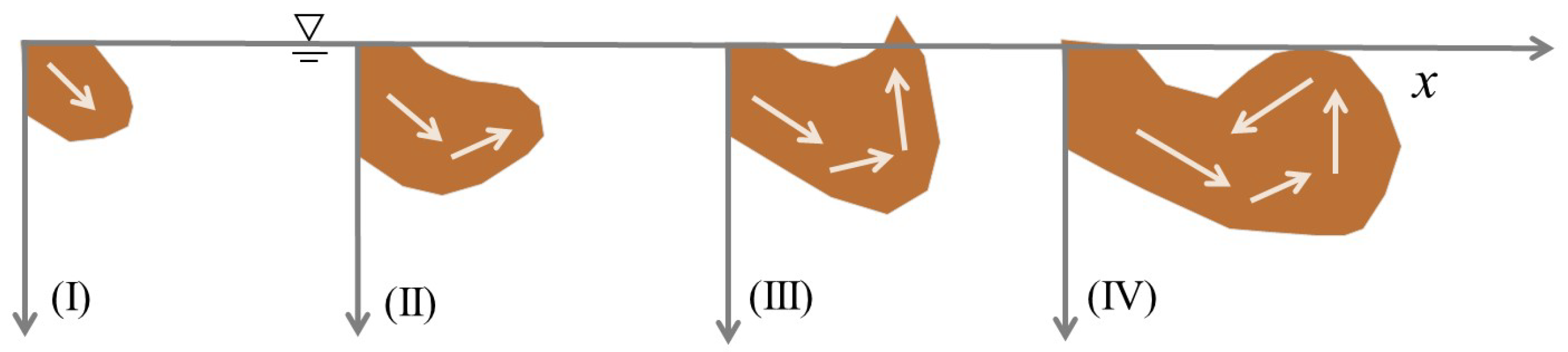
On the whole, the evolution of the center of mass was dominated by two factors: one was the volume of the submerged slide, which had a linear relation with the effective slide mass $m_E$; another was the deformation of the submerged slide, which resulted in $C_x<C_y$, during the impact. The evolution, of the frontal and deepest points, was related to the slide–water interface, which revealed the right and bottom boundaries of the submerged slide, respectively. Once it entered the water body, the slide moved along the slope at the very beginning, and the frontal part of the slide moved upward soon after, due to the buoyancy effect; then, it bent toward the shoreline, due to the resistance of water. Figure 9 illustrated the sketch of how the slide was deformed, since it emerged into the water body, due to the buoyancy effect and drag force.

Even though quantifying the submerged slide’s moving trajectory, by three control points, may involve an over-simplification, it, still, provided several interesting findings. First, the slide deformation almost followed the same tendency, in all experiments. Even the time nodes, during the evolution of the scaled coordinates of the control points, were similar for all experiments. Two significant time nodes were observed: one was T∼1, and another was T∼2. Almost all the curves increased very quickly at the very beginning at $T<1$, and increased with a decelerating trend at $T<2$, before they began to flatten after $T<2$. In addition, the slope angle was fixed to 45${}^{\circ }$, while our results showed that $C_x$ was significantly smaller than $C_y$, which demonstrated that the slide has a significant deformation upward, once it entered the water body. In addition, with the increase in P${}_E$, the control points’s coordinates increased on the whole. The slide’s deformation was more obvious with larger P. High deformability may reduce the efficiency of momentum transfer, from the sliding mass to the body of water.

3.3. Quantitative Analysis

The evolution of $C_x\left(T\right)$, $C_y\left(T\right)$, $D_x\left(T\right)$, and $L_y\left(T\right)$ reveals the overall and space-averaged motion of the submerged sliding mass. As shown in Figure 7 and Figure 8, the evolution of all the scaled coordinates of the control points are related to the impulse product parameter P. Accordingly, we presumed that the scaled coordinates of the control points at an indicated time can be fit with the impulse product parameter P. For the evaluation of the wave characteristics, researchers, commonly, simplified the predictive model and quantified the maximums of the wave parameters, such as maximum wave amplitude and maximum wave height, rather than the time series data. Quantifying the coordinates of the control points at the moment when the wave height reaches its maximum could be of interest for further analysis of the maximums of the wave parameters.

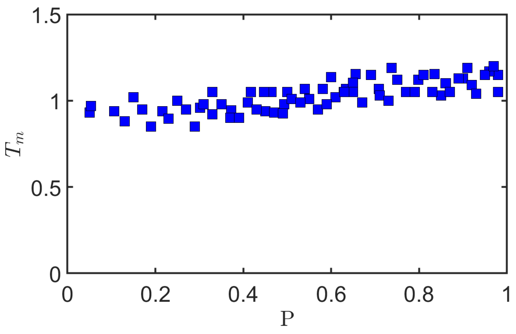
First, we defined the time taken, from the slide’s front entering the water body to the leading wave reaching its maximum height, as effective time $t_m$. Then, we scaled $t_m$ as $T_m=t_m{(g/h_0)}^{1/2}$, and defined $T_m$ as scaled effective time. As a first step, we determined the scaled effective time $T_m$ for each experiment. As shown in Figure 10, we found that the leading wave observed in most experiments arrives at its maximum height, approximately at the same time $T_m$∼1. With the increase in P, $T_m$ the has a slight increasing tendency. Interestingly, T∼1 was one of the important time nodes that was observed in the time evolution curves, in Section 3.2.

To provide a quantitative analysis, we collected the scaled coordinates of the control points at the moment $T_m$ and defined them as: scaled coordinate of the center of mass $(C_{x,m},C_{y,m})$, scaled horizontal coordinate of the frontal point $D_{x,m}$, and scaled vertical coordinate of the deepest point $L_{y,m}$. We then fit these parameters with the impulse product parameter P. Our previous study has demonstrated that the wave features including the scaled maximum wave height $H_m$ and scaled maximum wave amplitude $A_m$ can, also, be well fit with P for experiments conducted using Carbopol [22]. Figure 11a,b displays $(C_{x,m}$ and $C_{y,m})$ versus P. The solid line and the dashed lines denote the fitting curve and the ±30% derivation range, respectively. The best fitting equation for $C_{x,m}$ was:

$$C_{x,m}=0.6795{\mathrm{P}}^{0.5170}$$

(5)

and the best fitting equation for $C_{y,m}$ was:

$$C_{y,m}=0.2115{\mathrm{P}}^{0.4093}$$

(6)

with the coefficient of determination $R^2$ for Equation (5) and Equation (6) as 0.903 and 0.897, respectively.

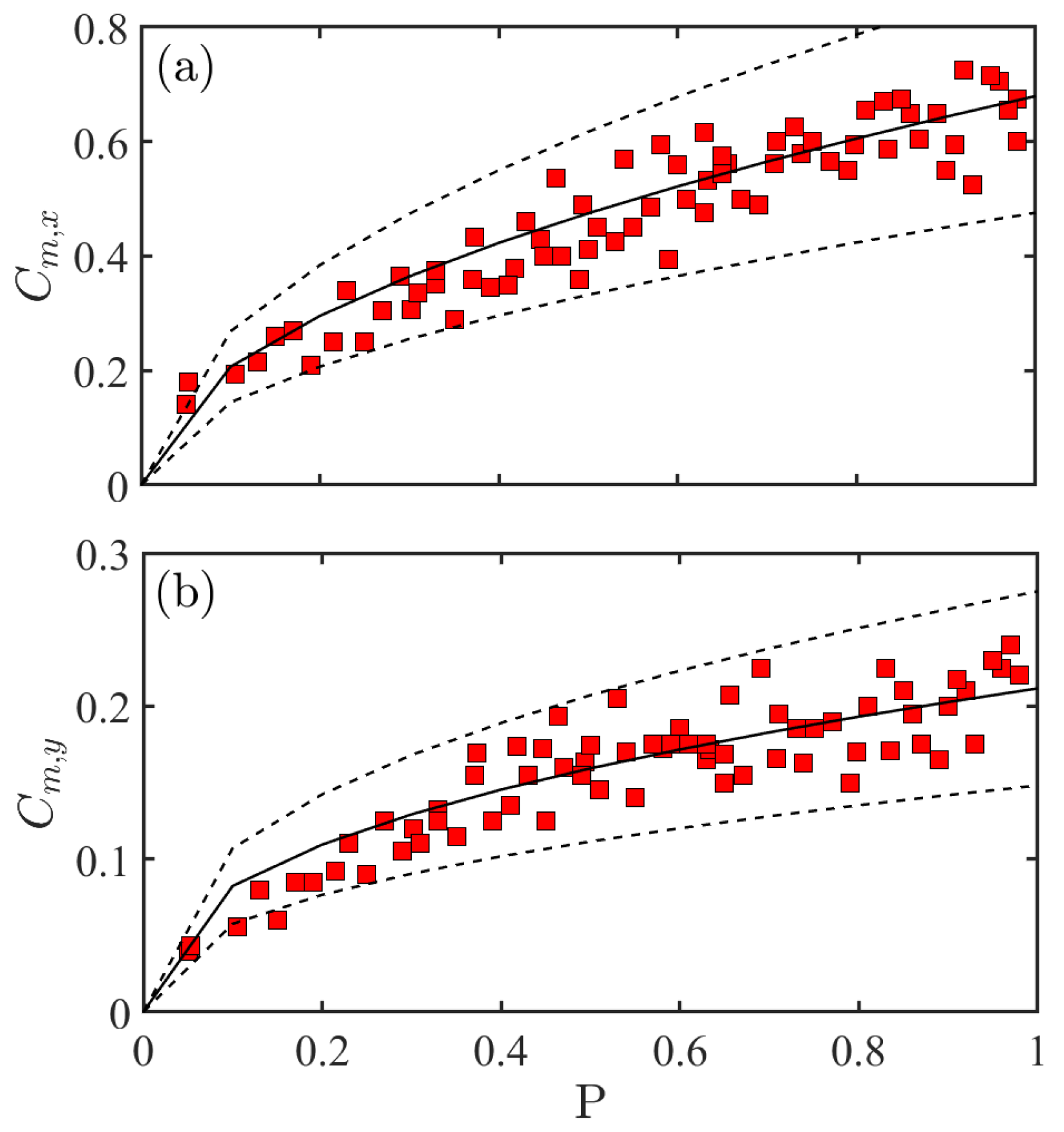
Figure 12a,b illustrates the variation of $D_{m,x}$ and $L_{m,y}$ with P, respectively. The best-fitting equation for $D_{x,m}$ was:

$$D_{x,m}=0.9115{\mathrm{P}}^{0.5080}$$

(7)

The best fitting equation for $L_{y,m}$ was:

$$L_{y,m}=0.4471{\mathrm{P}}^{0.4726}$$

(8)

The coefficient of determination $R^2$, for the fitting equations of $D_{x,m}$ and $L_{y,m}$, was 0.914 and 0.907, respectively.

The error range of most experimental data was within ±30% for Equations (5)–(8). Moreover, the coefficient of determination $R^2$ for these four equations was larger than 0.8. It means that $C_{x,m}$, $C_{y,m}$, $D_{x,m}$, and $L_{y,m}$, at the moment $T_m$, can be well fit with the impulse product parameter P, in the format $X=\alpha {\mathrm{P}}^{\beta }$, where $\alpha$ and $\beta$ are constant, and $X=C_{x,m}$, $C_{y,m}$, $D_{x,m}$, and $L_{y,m}$. The motion of the submerged sliding mass is dominated by the interaction force, between the slide and water, and can be considered as an intermediate process of the momentum transfer process and wave generation. This explains why both the wave features and the motion of the submerged slide can be well fit with P. This, also, shows the necessity of considering the motion and deformation of the submerged slide in wave prediction.

4. Conclusions

This study gave insights, into the motion and deformation of viscoplastic fluid while entering a body of water, and ran experiments using a viscoplastic material, called Carbopol. Comparing with experiments conducted with granular slides, our experiments observed a clear slide–water interface. We selected three specific control points, including center of mass, frontal point, and deepest point, to simplify the physical process of the submerged slide motion, in which the center of mass revealed the space-averaged slide motion, and the frontal and deepest points denoted the slide’s overall motion. The time evolution of the scaled coordinates of the center of mass ($C_x$, $C_y$), scaled horizontal coordinates of the frontal point $D_x$, and scaled vertical coordinates of the deepest point $L_y$ were determined, experimentally.

Instead of using an analytical method, proposed by Zitti et al. (2017), to analyze the submerged slide motion [15], we simplified the analysis and quantified the motion of the submerged sliding mass, as the support of the impulse product parameter P. Three interesting findings can be concluded from this study. First, the impulse product parameter P could not only quantify the wave features but also reflect the motion of the submerged sliding mass. Second, $C_x\left(T\right)$, $C_y\left(T\right)$, $D_x\left(T\right)$, and $L_y\left(T\right)$ increased with the increasing of P. Third, the scaled coordinates, at the moment when the wave height arrives at its maximum, $C_{x,m}$, $C_{y,m}$, $D_{x,m}$ and $L_{y,m}$, were well fit with P, with the coefficient of determination $R^2>0.8$ and the error range for most experimental data within ±30%.

References

1. Genevois, R.; Ghirotti, M. The 1963 vaiont landslide. Giornale Geol. Appl. 2005, 1, 41–52. [Google Scholar]
2. Ciabatti, M. La Dinamica Della Frana del Vajont; Museo geologico Giovanni Capellini: Bologna, Italy, 1964. [Google Scholar]
3. Vacondio, R.; Mignosa, P.; Pagani, S. 3D SPH numerical simulation of the wave generated by the Vajont rockslide. Adv. Water Resour. 2013, 59, 146–156. [Google Scholar] [CrossRef]
4. Gylfadóttir, S.S.; Kim, J.; Helgason, J.K.; Brynjólfsson, S.; Höskuldsson, Á.; Jóhannesson, T.; Harbitz, C.B.; Løvholt, F. The 2014 Lake Askja rockslide-induced tsunami: Optimization of numerical tsunami model using observed data. J. Geophys. Res. Ocean. 2017, 122, 4110–4122. [Google Scholar] [CrossRef] [Green Version]
5. Gauthier, D.; Anderson, S.A.; Fritz, H.M.; Giachetti, T. Karrat Fjord (Greenland) tsunamigenic landslide of 17 June 2017: Initial 3D observations. Landslides 2018, 15, 327–332. [Google Scholar] [CrossRef]
6. Kamphuis, J.; Bowering, R. Impulse waves generated by landslides. Coast. Eng. 1970, 575–588. [Google Scholar]
7. Heller, V.; Hager, W.H. Impulse product parameter in landslide generated impulse waves. J. Waterw. Port Coast. Ocean Eng. 2010, 136, 145–155. [Google Scholar] [CrossRef]
8. Mohammed, F.; Fritz, H.M. Physical modeling of tsunamis generated by three-dimensional deformable granular landslides. J. Geophys. Res. Ocean. 2012, 117. [Google Scholar] [CrossRef] [Green Version]
9. Heller, V.; Hager, W.H. A universal parameter to predict subaerial landslide tsunamis? J. Mar. Sci. Eng. 2014, 2, 400–412. [Google Scholar] [CrossRef] [Green Version]
10. McFall, B.C.; Mohammed, F.; Fritz, H.M.; Liu, Y. Laboratory experiments on three-dimensional deformable granular landslides on planar and conical slopes. Landslides 2018, 15, 1713–1730. [Google Scholar] [CrossRef]
11. Mulligan, R.P.; Take, W.A. On the transfer of momentum from a granular landslide to a water wave. Coast. Eng. 2017, 125, 16–22. [Google Scholar] [CrossRef]
12. Bullard, G.; Mulligan, R.; Carreira, A.; Take, W. Experimental analysis of tsunamis generated by the impact of landslides with high mobility. Coast. Eng. 2019, 152, 103538. [Google Scholar] [CrossRef]
13. Zitti, G.; Ancey, C.; Postacchini, M.; Brocchini, M. Impulse waves generated by snow avalanches: Momentum and energy transfer to a water body. J. Geophys. Res. Earth Surf. 2016, 121, 2399–2423. [Google Scholar] [CrossRef]
14. Fuchs, H.; Winz, E.; Hager, W.H. Underwater Landslide Characteristics from 2D Laboratory Modeling. J. Waterw. Port Coast. Ocean Eng. 2013, 139, 480–488. [Google Scholar] [CrossRef]
15. Zitti, G.; Ancey, C.; Postacchini, M.; Brocchini, M. Snow avalanches striking water basins: Behaviour of the avalanche’s centre of mass and front. Nat. Hazards 2017, 88, 1297–1323. [Google Scholar] [CrossRef]
16. Yavari-Ramshe, S.; Ataie-Ashtiani, B. On the effects of landslide deformability and initial submergence on landslide-generated waves. Landslides 2019, 16, 37–53. [Google Scholar] [CrossRef]
17. Miller, G.S.; Andy Take, W.; Mulligan, R.P.; McDougall, S. Tsunamis generated by long and thin granular landslides in a large flume. J. Geophys. Res. Ocean. 2017, 122, 653–668. [Google Scholar] [CrossRef]
18. Yin, Y.; Wang, L.; Zhang, W.; Zhang, Z.; Dai, Z. Research on the collapse process of a thick-layer dangerous rock on the reservoir bank. Bull. Eng. Geol. Environ. 2022, 81, 109. [Google Scholar] [CrossRef]
19. Bates, B.M. Fluid Dynamics of Basal Entrainment by Geophysical Gravity-Driven Flows. Ph.D. Thesis, Swiss Federal Institute of Technology Lausanne, Vaud, Switzerland, 2015. [Google Scholar]
20. Ancey, C. Plasticity and geophysical flows: A review. J. Non-Newton. Fluid Mech. 2007, 142, 4–35. [Google Scholar] [CrossRef]
21. Yavari-Ramshe, S.; Ataie-Ashtiani, B. Numerical modeling of subaerial and submarine landslide-generated tsunami waves-recent advances and future challenges. Landslides 2016, 13, 1325–1368. [Google Scholar] [CrossRef]
22. Meng, Z. Experimental study on impulse waves generated by a viscoplastic material at laboratory scale. Landslides 2018, 15, 1173–1182. [Google Scholar] [CrossRef]
23. Meng, Z.; Ancey, C. The effects of slide cohesion on impulse-wave formation. Exp. Fluids 2019, 60, 151. [Google Scholar] [CrossRef]
24. Meng, Z.; Hu, Y.; Ancey, C. Using a Data Driven Approach to Predict Waves Generated by Gravity Driven Mass Flows. Water 2020, 12, 600. [Google Scholar] [CrossRef] [Green Version]
25. Cochard, S.; Ancey, C. Experimental investigation of the spreading of viscoplastic fluids on inclined planes. J. Non-Newton. Fluid Mech. 2009, 158, 73–84. [Google Scholar] [CrossRef]
26. Bonn, D.; Denn, M.M.; Berthier, L.; Divoux, T.; Manneville, S. Yield stress materials in soft condensed matter. Rev. Mod. Phys. 2017, 89, 035005. [Google Scholar] [CrossRef] [Green Version]
27. Balmforth, N.; Craster, R.; Perona, P.; Rust, A.; Sassi, R. Viscoplastic dam breaks and the Bostwick consistometer. J. Non-Newton. Fluid Mech. 2007, 142, 63–78. [Google Scholar] [CrossRef] [Green Version]
Figure 1. The spread of granular particles in water.
Jmse 10 00778 g001
Figure 2. The sketch of the physical process of landslide-generated waves.
Jmse 10 00778 g002
Figure 3. The (a) sketch and (b) photo of the experimental facilities.
Jmse 10 00778 g003
Figure 4. Raw images of the selected experiment, recorded by the high-speed camera.
Jmse 10 00778 g004
Figure 5. The position of the selected control points: center of mass ( c x , c y ), frontal point ( d x , d y ), and deepest point ( l x , l y ).
Jmse 10 00778 g005
Figure 6. Time evolution of the (a) center of mass ( c x , c y ) and (b) mean velocity of the submerged slide u ¯ s . The time span δ t between each rhombus was 0.1 s.
Jmse 10 00778 g006
Figure 7. Time evolution of the scaled coordinates of the center of mass: (a) C x ( T ) and (b) C y ( T ) .
Jmse 10 00778 g007
Figure 8. Time evolution of the scaled horizontal coordinate of the frontal point D x ( T ) and the scaled vertical coordinate of the deepest point L y ( T ) .
Jmse 10 00778 g008
Figure 9. Sketch of the submerged slide’s moving and deforming process.
Jmse 10 00778 g009
Figure 10. The variation of the scaled effective time T m with P.
Jmse 10 00778 g010
Figure 11. Variation of (a) C m , x and (b) C m , y with P. The solid line and the dashed lines denote the fitting curve and the ±30% derivation range, respectively.
Jmse 10 00778 g011
Figure 12. Variation of (a) D m , x and (b) L m , y with P, for all experiments. The solid line and the dashed lines denote the fitting curve and the ±30% derivation range, respectively.
Jmse 10 00778 g012