Abstract
Most of the research on ship rolling motion concerns a specific type of ship, such as containerships, or analyzes sailing during certain wave characteristics, rather than the full spectrum of waves that can be encountered during the entire sea route. To date, the most frequent merchant ships in the world are general cargo ships, where the ship’s behaviour at any sea condition has a great influence on overall safety, as well as the lashing design of non-standardized cargo. For this reason, the present paper aimed to study ship-performance models, starting with concepts of the basic physics of ships and waves. Firstly, the ship’s behaviour was analyzed from a theoretical point of view, both in calm waters and when sailing in waves, but independently. Afterwards, the ship-waves system was analyzed during rolling with all variables accounted for at the same moment, with the objective of obtaining roughly realistic models. Relevant results are shown in each of the models, which may be of great interest for ship operators and, in general, for the shipping industry, so as to improve the safety of maritime transport. Finally, these results were validated with a case study.
1. Introduction
General cargo ships represent the most common ship types in the world, next to fishing vessels [1,2]. Although a high percentage of losses and cargo claims of all merchant ships are associated with general cargo ships, they are not considered by the general public and even by many authorities, as risky ships, maybe because such accidents have not had as much of a media impact as other cases [3]. Moreover, most of the accidents and causalities are related to rolling motion, which, in some cases, leads to a loss of stability with consequences on the ship, the cargo, the crewmember and the environment [4]. So, it is clear that it is of the utmost relevance to assess and predict a ship’s behaviour during the roll motion in any sea condition, as it directly influences, for example, the cargo-securing system, because stowage and cargo security is determined by the worst condition of acceleration and the rolling angle expected during the sea route [5].
The non-standardized cargo onboard ships has to be protected against forces generated during sea navigation, motions of the ship, waves and wind. The influence of waves and wind is applicable only to cargo stowed above the main deck, and according to the literature [6], its influence compared to other forces exerted against the cargo is relatively minor. Of the six-degrees of freedom of a ship in a seaway, the most important from the point of view of acceleration is the rolling motion which depends directly on the sea state [4,7,8], which is why it is the motion studied in this paper. The importance of this motion is reflected in the investigation of Li et al. (2021) [9], where they studied how to utilize the mechanical energy of this movement by means of an energy-harvest unit installed onboard. Therefore, today, it is clear that it is of utmost importance to study this motion in ships with thousands of oscillations when rolling throughout the day, for energy conservation and emission reduction onboard ships, representing a subject which has attracted attention across the board.
To date, the majority of research about ship acceleration and the rolling angle of ships sailing in waves concerns containerships, specifically, the parametric roll resonance phenomenon [10,11,12]. In the literature, many works and experiments that predict the rolling motion with numerical calculations and small-scale models in tanks where waves and wind conditions are artificially generated are reviewed and the results are contrasted using large-scale models during sea trials. However, this research is only applicable to certain types of ships (containerships and tugs) [11,13] or to very particularized sea states (short or long-crested seas) [8]. Another example of this trend is the work of Pesman (2016) [14], where the author analyzes ways in which ship operators of any ship can avoid or reduce the influence of parametric roll accelerations when sailing in longitudinal waves. So, although work in the literature about general cargo vessels is limited with regard to a certain loading condition and when sailing in waves, providing an understanding of the ship-roll motion when sailing in waves for shipmasters and operators is important in terms of stability, cargo security and, in general, the safety of the shipping industry. In this sense, recently, authors such as Acanfora and Balsamo [15] presented their research in which a numerical model was developed in order to detect the synchronism and the parametric roll. In their work, maneuvering equations were implemented which consider the ship dynamics in waves in order to act accordingly to reduce large roll motions with alerts provided by an autonomous detection system. The ship used in the case study was a ro-ro pax vessel, i.e., the other type of ship (together with pure container ships) more vulnerable to these phenomena. However, as mentioned, it is not necessary to reach the synchronism or parametric roll in order to put the ship’s safety at risk, and for anticipating the phenomenon, it is necessary to know the ship’s behavior in all sea-state conditions.
Concerning the condition of the sea state used in the present study, the wave-induced motion of abeam seas was considered as trochoidal regular. This is in accordance with the procedures followed by other authors [16,17] in previous research investigating similar problems. In these works, the authors mentioned that the irregular natural seaway is modelled as a superposition of waves of different characteristics (wavelength and period), and for that reason, a set of regular waves, for which the natural seaway is superimposed, were used in the computer calculations. This is because, as is apparent, the identification of the real sea state parameters is not a simple task due to the interaction between short-crested waves and swell waves. Jiao et al. (2019) [8] carried out an in-depth study on ship motion sailing in short-crested irregular waves but by considering a model of a length greater than 300 m, which is outside of the range of most general cargo ships that transport non-standardized cargo. Furthermore, the research focused on specific types of waves (short-crested or long-crested), however, it is not possible to predict what types of waves will be encountered during the sea route, because weather forecasts often only include the height and/or period of waves. Other authors, such as Zakaria (2009) [18], also carried out relevant research about the effect of irregular waves and severe sea states (moderate gale, strong gale and hurricane) on ships but, once again, in certain containerships, with numerical calculations in order to consider resilience in the stage of ship design. In this study, simulations were used to analyze three specific sea states, and although this was intended to reflect the worst conditions, it is a very restrictive consideration of general shipping operations. In connection with the ship-design phase, Zhang et al. (2021) [19] applied a new, three-dimensional time-domain panel method to solve and predict, in this initial stage, the hydrodynamic seaworthiness of the ship in the wave–ship system, but not in the daily operation of the ship to ensure that it, together with the transported cargo, remains in good seaworthy condition. Regarding research conducted with CFD tools, the work of Huang et al. (2021) proves interesting [20], where the effects of different states on the motion stability of an unmanned surface vessel were investigated, specifically of a catamaran. However, the investigation did not consider, for example, the ship’s loading condition and reached the conclusion that overturning did not occur, which shows that the full spectrum of the sea state was not analyzed.
Furthermore, ships need to satisfy several regulations, guidelines, procedures and standards approved by the classification society in charge and/or the authority of the flag state. This aspect also affects the stowage and securing of cargo so that it is transported with a high level of safety. Several works, such as that of Petacco and Gualeni (2020) [21] and Marlantes et al. (2021) [22] pointed out that IMO (International Maritime Organization), through IS Code version 2020 (International Code on Intact Stability, 2008), implemented guidance and operational limitations during navigation for a stability assessment. This new version of IMO Code addresses the ship stability condition when sailing in waves, but only refers to five dynamic phenomena, i.e., parametric roll, pure loss of stability, dead-ship condition, surf-riding and excessive accelerations (weather criterion). Taking into account this last concept, and after analyzing the IS Code 2020 [23], it can be concluded that it addresses the maximum rolling angle in the zero-speed condition and under the action of pure beam seas, but does not specify the sea state or the wind intensity, so the available margin of safety in case of encountering extreme weather conditions is unknown. Before the introduction of IS Code version 2020, research [24] had already been carried out to predict the rolling motion (period) following to IMO formula and using the GZ curves of different ships. The main objective was to avoid the greatest threat to the ship’s stability and safety, i.e., the resonance of rolling, although, as it is known, it is not only this extreme circumstance that threatens the ship’s safety.
Therefore, considering all of the above, the cargo should be stowed and secured in a safe manner if the ship is going to sail in an area with a specific sea state (undetermined), but if the weather conditions are different, the overall safety of the ship could be compromised, as none of these calculations include any meteorological parameters. When a ship sails in waves, it acts as a floating beam on which a set of forces varying in time act. This ship motion in waves is a feature that has negative influences on various parameters, causing, among other effects, a decrease in stability, increased stresses on the hull and relevant forces on the cargo. So, motions of excessive amplitudes can become very dangerous for the seakeeping and general safety of ships and cargo. For this reason, in the present paper, we intended to include the main sea conditions affecting the ship roll motion, which affects the ship’s general behaviour, including the cargo stowage and lashing design. Related to this point, it is also important to note that some boards for classification, such as DNV·GL [25], provide guidelines of default motion criteria in different sailing areas. For example, the single amplitude of rolling can be read as a constant and particulars of the navigation areas for ships are predefined. However, it is considered necessary to carry out a theoretical and realistic study about roll motion models based on the ship’s particulars and all specific conditions of the waves, which on a specific sea passage can be different from the annual statistics.
Therefore, the aim of this paper is to carry out an analytical study of the ship’s performance during the roll motion from a theoretical and realistic point of view, and with regard to any sea condition that can be encountered during sea passage across world, regardless of the ship’s particulars and the waves’ conditions, with the objective of guaranteeing a required level of safety and preventing damages, losses and claims. Finally, in each section, our results are validated with a case study.
2. Materials and Methods
In the present research, the ship motion studied is the rotational motion around the longitudinal axis, that is, the rolling motion. For that, in this section the different mathematical models applied to rolling are independently analyzed. Firstly, a model of a ship’s rolling oscillating freely is studied in calm conditions and as a consequence of the application of a punctual and external force, which produces a roll due to the ship’s loading condition, expressed as a natural roll period (Td). Afterwards, a mathematical model of regular waves corresponding to any sea state conditions, expressed as the wave’s period (Tw), is studied, in order to apply such a model in a mathematical model of the ship’s rolling motion when sailing between waves of abeam seas. These analyses will be used as tools to develop an understanding of the real ship’s behaviour during navigation. However, as there is a lack of tools available to define the behaviour of ships under these conditions, in the results section, the results will be analyzed to produce an approximate realistic model. In the present work, only the influence of waves acting perpendicular to the ship’s centreline is studied because, in a zero speed condition, such waves represent the worst condition in the ship rolling motion, and we aim to find the extreme values during rolling motion.
Regarding the pitching motion, due to the large torque of a ships’ longitudinal stability, it would be difficult, if not impossible, to cause a free longitudinal oscillating motion with a punctual force. This aspect would lead to overlooking the pitch motion in calm waters and, even with the ship sailing in regular waves, it would introduce some difficulty because when the ship is sailing in ahead/stern seas, the wave’s profile cannot be replaced by a straight line (as in the rolling motion study) due to the usual relationship between the ship’s length and the wavelength.
2.1. Ship’s Rolling Motion in Calm Waters
In the first stage of the present study about ship motion when sailing in waves, it was considered necessary to represent the free rolling motion of the ship in calm waters and without water resistance, as it would represent the worst condition. It is relevant to note that when a stable idle ship is displaced from its equilibrium position by some external force, when the induced force stops, the ship will oscillate until the resistance of water dampens the motion.
The defining equations of the ship rolling motion in calm waters include the equations of a vibratory system, which is used for the assumption of a ship oscillating without damping, i.e., without considering the resistance of the water, the calculations will only correspond to a simple harmonic motion [4].
An interesting formula for shipping operators is one that links the (double) natural rolling period (Td) of the ship with the initial transverse metacentric height (GM), accounting for the radius of the gyration of the ship’s mass. The deduction starts with the equation of the motion of a solid rotating around an axis, which has the following expression [26]:
where Ig is the inertia moment of the ship’s mass about a longitudinal axis through its center of gravity; θ is the rolling angle and d2θ/dt2 is the angular acceleration.
According to this approach, Equation (1) is equal to the righting moment of the ship; therefore, its algebraic sum will be equal to zero. After altering Equation (1) to consider the GM and ship’s displacement, the following equation is obtained:
where k is the turning radius of the ship’s mass with respect to the longitudinal axis passing through its center of gravity and g is the gravity acceleration.
Equation (2) is the same type as an Equation of simple harmonic vibratory motion, which corresponds with the differential equation of rolling motion, as follows:
In order to calculate the constants AK and BK of the solution, a general condition is assumed for when the time (t) is equal to zero (t = 0), so θ = φ, and therefore:
In Equation (3) when t = 0, the value of the constant AK is:
In order to obtain the value of the constant AK, Equation (3) is derived:
Therefore;
Clearing AK,
By replacing the constants AK and BK for the calculated values in Equation (3), the following differential Equation can be obtained:
However, knowing that the angular velocity [27] is as follows:
The constant AK of Equation (9) takes the following expression:
Additionally, by introducing the angular velocity dφ/dt, it takes the form:
Therefore, Equation (10) is transformed into the following equation:
Finally, the equation of rolling motion in calm waters can be expressed as follows:
2.2. Waves
The transverse roll motion of ships is produced due to constant changes in the apparent vertical direction along with the trochoidal profile of waves, where the ship’s diametrical plane tries to follow their profile in order to reach the equilibrium position. When the waves pass along the ship, a motion in the centre of the buoyancy of the ship is produced, leading to a hydrostatic restoring moment of the stability in waves, which attempts to keep the ship upright and leads to the rolling motion. Then, the absolute amplitude of the rolling motion depends on the following two factors: the relative position of the ship’s diametrical plane with respect to the apparent vertical direction and, the relative position of the apparent vertical with respect to the true vertical. As consequence, the roll motion depends on the ship’s oscillation movement and the waves’ undulatory motion, i.e., on the ship roll natural period (Td) and the waves’ period (Tw). Depending on whether these periods are more or less concordant, they will cause the amplitude of the absolute roll to be increase or decrease. Therefore, it is very important for deck officers to have an understanding of the natural rolling period of their ships for that oscillation mode.
In the study of the waves, it is referred to the waves of theoretical or tended regular sea (after the wind ceases), when its profile corresponds to a trochoid curve because the ship motion in irregular seas is impossible to accurately predict [28]. These waves are the only ones that have been able to be studied mathematically, based on the properties of the trochoid, from direct observation, and regardless of the resistances that water molecules encounter in their movement.
When studying the trochoidal waves profile, there are different formulas that can be used to establish a relationship between wavelength, translation speed and period of waves [29]. Moreover, recent studies that include all seas in the world have helped in building a scale of 21 types of waves with these three parameters. Considering the values of wavelength and period, a polynomial regression equation (Equation (16)) with a precision of 100% for the determination factor was obtained. Figure 1 is shown a good relationship between wavelength and period parameters.
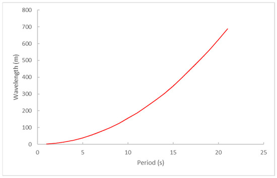
Figure 1.
Representation of wavelength as a function of period.
However, there are no formulas that relate these three parameters with the height (Hw) (or amplitude-Aw) of the waves due to the dependence of height on other variable factors such as the fetch and the duration of the wind influencing the fetch. Nevertheless, the maximum wave slope (α) is related to the wave height (Hw) and the wavelength (Lw) according to the following Equation (17):
Other authors [30] have registered the wavelength, the height and the period of waves all over the world, and found that the value of sin (α) is almost constant and equal to 0.1047, i.e., α = 6°, regardless of smooth or very rough sea. For this reason, the relationship between wavelength and height can be considered as constant according to Equation (18).
Using Equation (18) and the wavelength (Lw), which was expressed according to Equation (16), the waves’ height (Hw) as a function of the wavelength and the wave period (Tw) can be calculated. Furthermore, it is possible to obtain the amplitude (Aw) of the wave, knowing that this parameter is equal to half of the height (Hw) [31].
In Table 1, all variables calculated according to Equations (16)–(18) and considered in the present study are included, which correspond to the full the spectrum of regular waves:

Table 1.
Data of studied waves.
Finally, having tabulated the obtained data, which are included in Table 1 with respect to the wind force that generates a specific sea condition, in Table 2, the Beaufort scale, the wind mean velocity (Vw) and the corresponding waves’ maximum height (Hw) are included [29].
Table 2.
Influence of wind intensity on waves’ height.
2.3. Ship’s Rolling Motion Sailing in Regular Waves
In calm water conditions, the buoyancy of the water acts perpendicularly to the water line surface according to the vertical and, when the surface comprises a trochoidal wave, the buoyancy of the water changes constantly. For this reason, in the first case, the ship receives a constant buoyancy while, in the second, it varies continuously both in intensity and direction.
When a wave hits the ship, a disruptive force will be produced and it will change the underwater hull form. Consequently, the righting moment of the ship will try to find the equilibrium in the perpendicular direction of the trochoid, which changes constantly in terms of direction. After considering rolling in calm waters and the angle of the trochoid slope, the following equation of rolling as a function of the frequencies of the ship and the wave as can be deduced:
The first two terms of Equation (19) are the differential equations of the simple harmonic motion, and the third term is the disruptive force of the wave where , the maximum angle of the wave’s slope, can be expressed as follows:
where Aw is the amplitude of the wave (half the height, Hw) and Lw is the wavelength.
In order to calculate the disruptive force of the wave, the following solution can be used:
Using Equation (21), the rolling angle with respect to time can be obtained:
By introducing the value of the acceleration in Equation (19), in which it was previously cleared by equalizing the two type of motions, i.e., rolling in calm waters and rolling produced by the disruptive force of waves, the following is obtained:
Knowing that:
Equation (33) gives the constant CK as a function of the maximum angle between the vertical and the normal direction to the wave’s slope, and the period of a ship’s rolling motion (Td) and the wave period (Tw). By replacing Equation (33) in Equation (21), the following is obtained:
Therefore, the solution of the rolling equation of the ship sailing in waves and in a non-resistant environment is:
Equation (35) can also be expressed as follows:
The first two terms of the second part of Equations (35) and (36) correspond to free motion according to the ship’s natural period (Td) for a certain load condition, and the third term corresponds to the action of the wave, as a function of the wave period (Tw). This last term produces the induced roll motion.
As a consequence, a more in depth analysis is needed and is provided in the results Section.
The ship’s characteristics are concentrated in the Td variable, i.e., in the ship’s loading condition, which depend on the ship’s breadth and the metacentric height (GM), as can be seen in the next Section.
3. Results
The theoretical–practical analysis of the ship motion in waves, although very useful, is subject to initial conditions and assumptions as is the case in many other fields. Therefore, it must be understood as an orientation of the ship’s seakeeping with pure beam seas.
This section provides a study of ships’ behaviour expressed as a function of the rolling angle, angular velocity and transverse acceleration. To do so, and following the approach proposed in this paper, the ship’s performance in calm conditions was theoretically analyzed, where the only parameters at play were the previous average roll angle and the ship’s loading condition (Td). In the second stage, the same procedure was followed, but applied to the ship motion when sailing in regular waves, from a theoretical point of view. Finally, and taking into account the two previous theoretical studies, the real ship’s behaviour when sailing in waves and considering all variables in play was investigated in order to obtain objective results applicable to any condition. In each of these sub-sections, relevant and objective results are shown.
3.1. Theoretical Understanding of Free Rolling Motion in Calm Waters
When the ship is in an upright position, the angular velocity in calm conditions (θ′CC) during the free rolling motion can be expressed as follows:
According to Equation (37), the maximum angular velocity is produced with a periodicity when the time is and the angular velocity is zero when t (time) is .
In addition, the transverse acceleration in calm conditions (θ′′CC) corresponds to the following expression:
As a consequence, the moments when the maximum accelerations are reached are equal to and the instants when the accelerations are zero correspond to .
In order to validate our results, three parameters (rolling, velocity and acceleration) were considering, including the following initial conditions:
- Ship in the upright position;
- 10° as the average angle of rolling and;
- A natural roll period of 12 s (Td).
The selected ship’s loading condition of Td = 12 s was calculated after analyzing the ship’s particulars in a representative number of coastal general cargo ships, which can be represented with a breadth (B) of 16 m and an overall length of 100 m. According to DNV·GL [32], GM for general cargo ships is about 0.07⋯B, i.e., in this case, GM = 1.12 m, and the natural roll period can be calculated as follows:
Therefore, according to Equation (39), Td = 11.79 s.
Furthermore, according to IS Code [23], the roll natural period can be calculated with the following Equation:
where
In Equation (41), d is the mean draft and Lwl is the ship’s length at waterline. Then, following Equations (40) and (41), and considering a usual mean draft of 5.0 m, the natural roll period for this case study is 11.95 s.
Moreover, as per Bonilla [30], it can be considered that for cargo ships, 10 s < Td < 14 s, and that 0.055 < GM/B < 0.080, and for the selected case study, 0.88 m < GM < 1.28 m. Then, considering a GM of 1.1 m (the same that above calculated), in which the ship would be in a representative condition, Td can be also obtained following Equation (42) [30], which would result in Td = 11.75 s:
Finally, Bonilla [30] considers that in normal circumstances, the Td of any cargo ship is between 10 s and 14 s, so the selected loading condition of 12 s could be considered representative enough, following which the model can be applied to any kind of ship.
As can be seen in Figure 2, the ship rolls freely in calm waters from one side to another with a constant amplitude over time, due to non-resistance. In this situation, the disturbing force would be an external and momentary force that produced a heeling torque opposed by the ship’s righting moment. In this situation, the maximum angle of the roll matches the moment when the maximum transverse acceleration is produced.
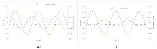
Figure 2.
Rolling motion in calm waters and without resistance. (a) Rolling angle and angular velocity vs. time (b) Rolling angle and acceleration vs. time.
With a frequency of the ship is in the upright position, with no angular acceleration, and it starts a new process of rolling to the opposite side, until completing the full oscillation, corresponding to the natural rolling period (Td). This rolling motion would be repeated indefinitely, however, it is realistic to assume that the water and the air resistance will absorb the rolling amplitude until the ship is again at an upright position and at rest [10].
As can be seen in both graphs of Figure 2, the instants when the maximum and minimum (zero) values are reached, reveal the precision of our results, as commented on previously.
3.2. Theoretical Understanding of Rolling Motion under Regular Waves’ Influence
The angular velocity (θ′W) produced by the influence of the induced-force of the waves only (independently of the ship’s own oscillation) in a ship with a certain loading condition (Td), can be calculated as follows:
From Equation (43) it is obtained that the maximum induced velocity is achieved when time and it is zero when time .
Likewise, the induced acceleration (θ″W) is determined as follows:
In this case, it can be deduced that the highest acceleration is reached when and it is minimal or zero when .
In addition to obtaining the rule that calculated the moment in which these extreme values occurs, it can be concluded that despite the fact that Equations of induced-rolling motion include the ship’s loading condition (Td), the maximum–minimum accelerations and angular velocities depend only on the sea state condition (Tw), and not on the ship’s natural rolling period (Td).
Once again, to put into perspective and validate our results, in Figure 3, the rolling motion induced by trochoidal waves of, for example, Tw = 8 s is represented. Here, it can be observed that the highest angle of rolling is produced at the same time that the highest acceleration occurs. Furthermore, it is shown that the maximum angular velocity is reached with the ship in the upright position and that when the ship has the maximum rolling angle, the angular velocity is zero.
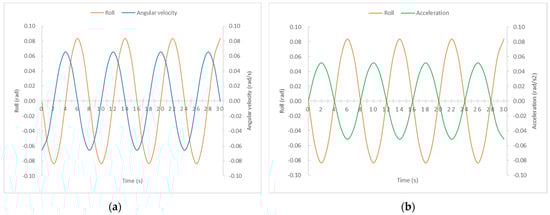
Figure 3.
Rolling motion induced only by waves of Tw = 8 s in a ship with Td = 12 s and without resistance. (a) Rolling angle and angular velocity vs. time (b) Rolling angle and acceleration vs. time.
3.3. Understanding of Real Behavior of Ship-Waves System Based on Theoretical Analysis
In this section, the ship’s performance is analyzed when sailing in waves, considering the ship’s free oscillation (Td) and the role played by the trochoidal waves of different characteristics during the rolling motion.
Considering Equation (36) which express the rolling angle equation of the ship sailing in waves, the total angular velocity in the ship–wave system can be calculated by deriving the rolling angle with respect to time. This angular velocity can be referred to as follows:
If θMW is expressed as a function of its variables, the Equation can be shown as:
Furthermore, the corresponding transverse acceleration, which can be obtained after deriving the rolling angle with respect to time twice, or after deriving the angular velocity with respect to time once, can be calculated as follows:
Unlike the results referred to in the previous sections, in this case, it is not possible to conclude directly the situations that produce the minimum and maximum values. Therefore, it is necessary to solve the following equation to calculate when zero acceleration is reached. To do so, it is sufficient to set the equation of transverse acceleration as equal to zero:
In addition, the moments when the highest (maximum) accelerations are produced can be calculated by deriving Equation (47) of transverse acceleration with respect to time once and when equal to zero, as it is represented in Equation (49):
In our validation process, in the first stage, as is represented in Figure 4, the breakdown of the rolling angle, angular velocity and transverse acceleration induced by the hitting of waves with a Tw = 8 s were calculated, with the ship rolling under free motion conditions and with the loading condition defined as Td = 12 s.
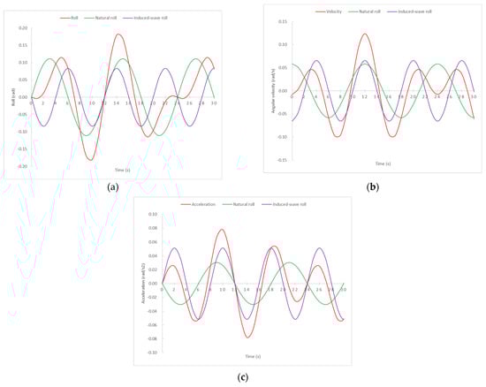
Figure 4.
Rolling angle (a), velocity (b) and acceleration (c) of a ship with a Td = 12 s sailing in waves of Tw= 8 s.
In this particular case of sea state, for example, it can be observed that the rolling and acceleration is zero when . However, the maximum velocity is not always reached in such specific conditions, as can be expected by analyzing the results of the previous Sections. For this reason, in the present research, we analyzed all sea state conditions that can be encountered by the ship during sea navigation, because they may be unknown or variable. In order to do so, it is necessary to know the accelerations trends produced by the 21 different sea conditions, based on 21 periods of waves (Tw). These accelerations are represented in Figure 5, where they are broken down as a function of the accelerations produced by 21 induced-waves (Tw) and the rolling natural period (Td) of 12 s, which, in real navigation, act as a joint system.
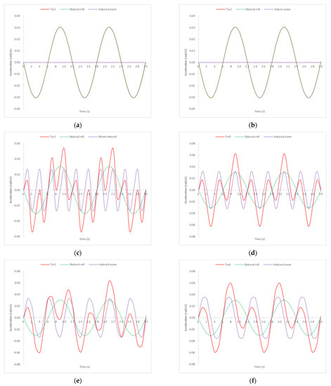
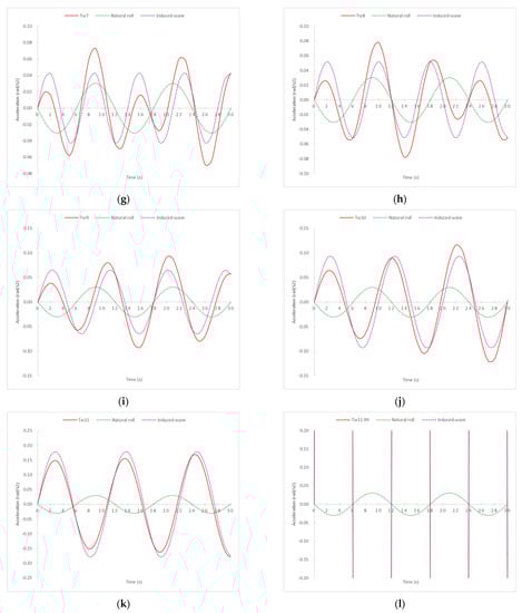
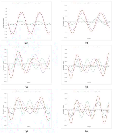
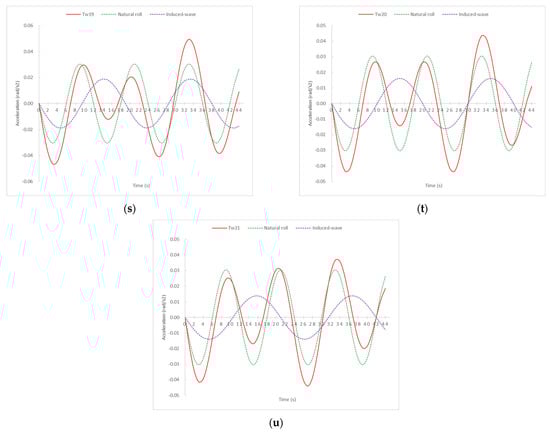
Figure 5.
Total transverse accelerations (red lines) by 21 different swell conditions for a ship with a Td = 12 s broken down into the sum of ship’s natural roll (green lines) and the induce-wave roll (purple lines). (a) Tw = 1 s (b) Tw = 2 s (c) Tw = 3 s (d) Tw = 4 s (e) Tw = 5 s (f) Tw = 6 s (g) Tw = 7 s (h) Tw = 8 s (i) Tw = 9 s (j) Tw = 10 s (k) Tw = 11 s (l) Tw = 11.99 s (m) Tw = 13 s (n) Tw = 14 s (o) Tw = 15 s (p) Tw = 16 s (q) Tw = 17 s (r) Tw = 18 s (s) Tw = 19 s (t) Tw = 20 s (u) Tw = 21 s.
Although there is no single trend or common pattern in all graphs, some remarkable conclusions can be extracted from Figure 5. Except for Tw = 12 s, which will be commented on in the next paragraph, and until Tw = 14 s (i.e., wavelength of 302 m and wave height of 10.06 m), the highest acceleration practically coincides with the moments of the highest acceleration produced by the waves’ acceleration components. From Tw= 14 s onwards, i.e., waves with the highest height and wavelength, the maximum acceleration tends to be convergent with the moments of the highest accelerations produced by the ship’s own oscillation (Td), within the full oscillation range (Td). Therefore, it can be concluded that, approximately, in the range of a Tw of between 3 s and 14 s, the moment of relative highest acceleration, within each oscillation at the same side, is registered when . As can be seen in the graphs, the sea states of Tw = 1 s and 2 s do not produce any motion due to their parameters of wavelength and height being very small. Furthermore, in the range of a Tw between 15 s and 21 s, it can be concluded that relative maximum accelerations within each oscillation occur when .
From Figure 5, it is also relevant to note that the most extreme accelerations are produced by Tw = 13 s and Tw = 11 s. The reason is that these sea condition values are close to Tw = 12 s, i.e., close to the natural rolling period of the ship considered in this simulation (Td = 12 s) and the occurrence of the synchronism phenomenon. What is more, when Tw = 11.99 s and with an amplitude and wavelength corresponding to Tw = 12 s, the curve acceleration is an asymptote curve, precisely due to the synchronism phenomenon where the rolling angles would continue to increase until the ship overturns. According to the same reasoning, and from a theoretical point of view, the same would occur for pitching motion when Tw approached the longitudinal natural period.
If the apparent period of the wave and the period of the ship are the same or almost the same (by excess or by default) in calm waters, theoretically, the ship will overturn, assuming the sea state as regular, the ship isochronous and in a non-resistant environment. However, in practice, different situations determine a resistance environment; the natural period of the ship, which increases with the rolling amplitude; and the irregular waves and the passive resistances, which increase with the square of the rolling amplitude. In any case, large rolling must be avoided due to the dangers of shifting some cargoes, the increased fatigue of ship structures and considerations of life on board.
All the above mentioned results can be applied when analyzing the range of highest and lowest angles of rolling, due to both parameters (rolling and acceleration) being sinusoidal functions.
In this study, it was shown that if a ship is subject to an induced roll motion due to the influence of regular pure beam waves, in the lower mid-range of Tw, as time goes on, the ship will roll according to the constant wave period (Tw) instead of rolling with its natural period (Td). However, because of a lack of regularity, both in space and time, and the ship’s tendency to roll according to its natural period, the period of roll motion of the ship will not be constant.
Furthermore, with the ship in a static condition (zero speed), if the angle of attack of waves is not perpendicular to the ship’s centreline, the absolute values reached during rolling motion would be lower.
4. Discussion
After analyzing the obtained results about the influence of different sea state conditions on the amplitude of rolling, velocity and transverse accelerations for a fixed Td (12 s), in order to understand the ship’s behaviour when sailing in a certain sea condition, several simulations for different ships-load conditions, specifically, Td = 10 s and Td = 14 s were carried out. These ship-loading conditions (represented in Figure 6) are the closest representative conditions of the simulations carried out previously, and represent those that the ship can reach after leaving port with a given stowage condition, in this particular case, Td = 12 s. For a general cargo vessel, a ship’s loading condition will be higher or lower than previously mentioned, and could be difficult to reach in real life in order to maintain the seaworthiness conditions and the safety of the studied ship because of an excess (Td too low) or lack of stability (Td too high).
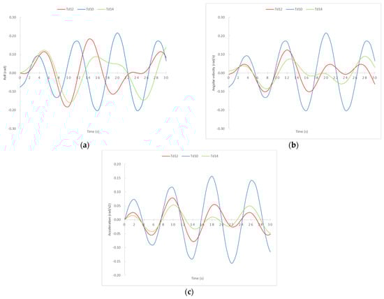
Figure 6.
Rolling angle (a), velocity (b) and acceleration (c) of a ship with different loading conditions (Td = 10, 12 and 14 s) sailing in waves of Tw = 8 s.
When the GM is high (Td low) in calm waters, the ship will experience few rolling motions, which will be short and fast. However, with this condition and when sailing between waves, the ship will have large absolute rolling angles, because a ship’s to have diametrical plane tends to coincide with the apparent vertical, which gives rise to large absolute rolling angles.
From Figure 6, it is observed that in the cases of the lowest GM (highest Td), the transverse acceleration is relatively low. The reaction of the ship to the rolling motion induced by the wave’s slope will be slow, tending to a small amplitude oscillation or, in other words, keeping the ship’s deck more or less horizontal, and not following the wave in its motion, which is not considered a good seaworthiness condition.
The use of diagrams in this study aimed to facilitate an easier decision-making process with regard to ship operability with regard to securing cargo, the best stowage position for a specific journey, for shifting some weight in order to improve the seaworthiness condition and to reduce the maximum transverse accelerations and rolling angle. They can help in making decisions when reaching a port of refuge in case of bad weather conditions where a shifting of weight does not satisfy the actual cargo lashing system. An easier decision-making process would influence the safety of the cargo, the crewmembers, the ship and the environment, enhance the comfort of crewmembers and reduce stresses on ship structures. However, in these calculations, we considered the worst condition of beam seas, at a zero-speed condition, without damping and in regular trochoidal waves. Any other combination would lead to a better performance of the ship when sailing in waves, so shipmasters and operators should also have relevant experience with which to recognize the subjective sea state.
5. Conclusions
In the present work, theoretical and realistic analyses of the ship’s rolling motion were conducted, investigating both the ship’s performance in calm conditions and when sailing in regular abeam waves. Finally, a study on the influence of the rolling motion in the ship–waves system was performed.
The results show that the highest angular velocity is reached when the ship rolls in calm waters, and , and as a consequence of the waves, only when . Zero angular velocity is reached when and , respectively. Furthermore, in calm waters, the maximum transverse accelerations is produced when , and due to the only influence of hitting of waves when . Zero accelerations are registered in calm conditions when , and under influence of waves when .
With respect to the maximum and minimum rolling angles, they follow the same pattern as transverse accelerations, because both are sinusoidal functions.
Although these theoretical results are applicable to any ship’s particular specifications and sea-state conditions, when both conditions were studied at the same time, according to our results, it was necessary to differentiate the sea conditions in order to predict the ship’s behaviour. For instance, in the range of a Tw from 3 s to 14 s (which corresponds to a wave height from 0.47 m to 10.06 m), the maximum accelerations almost coincide with the moment of the maximum acceleration produced by the wave, i.e., . However, for Tw = 14 s onwards, i.e., a wave height from 11.56 m to 22.91 m (Tw = 21 s), the maximum acceleration almost coincides with the instant of the maximum acceleration produced by the ship in calm waters, in this case, .
However, in all case studies, the synchronism phenomenon has to be considered, which is produced when the ship’s natural period (Td) and the wave period (Tw) are equal or almost the same, because in these conditions, the rolling angles increase until the ship overturns. Obviously, in this situation, none of our results would be valid.
All these results are valid considering certain initial conditions and assumptions such as a regular sea state, the ship being isochronous and a non-resistant environment. Therefore, future studies can be guided towards research about ship’s behaviour with a consideration of these mentioned variables, or assessments on how shipmasters and operators should proceed if in the middle of the voyage, the sea state worsens, in order to make safer and faster decisions in a timely manner.
Finally, as it was shown, in order to predict or improve the ship’s behaviour when sailing in regular abeam waves, or at the time of designing the lashing system of the cargo, the swell or sea state condition (Tw) has to be taken into account as well as the ship’s loading condition (Td), which can be adjusted during sea navigation by means of ballasting, deballasting of vertically transferring ballast water. Furthermore, considering these results, ship operators can pre-empt the worst and the best moments of rolling motion in order to act accordingly from a safety point of view.
Author Contributions
Conceptualization, J.M.P.-C. and J.A.O.; methodology, J.M.P.-C., J.A.O., F.F. and P.L.-V.; validation, J.M.P.-C., J.A.O., F.F. and P.L.-V.; formal analysis, J.M.P.-C., J.A.O., F.F. and P.L.-V.; investigation, J.M.P.-C. and J.A.O.; data curation, J.M.P.-C., J.A.O., F.F. and P.L.-V.; writing—original draft preparation, J.M.P.-C., J.A.O., F.F. and P.L.-V.; writing—review and editing, J.M.P.-C., J.A.O., F.F. and P.L.-V. All authors have read and agreed to the published version of the manuscript.
Funding
This research was funded by the R&D projects (Retos y Generación de Conocimiento) of the Spanish State Plan for Scientific and Technical Research and Innovation. Reference number PID2020-119639RB-I00.
Institutional Review Board Statement
Not applicable.
Informed Consent Statement
Not applicable.
Data Availability Statement
Not applicable.
Conflicts of Interest
The authors declare no conflict of interest.
References
- EQUASIS. The 2019 World Fleet Report. Statistics from Equasis. The World Merchant Fleet in 2019. Available online: http://www.equasis.org/EquasisWeb/public/HomePage (accessed on 13 May 2022).
- UNCTAD. Handbook of statistics 2021. Maritime transport. Merchant Fleet by Flag of Registration and by Type of Ship, Annual. Available online: https://unctad.org/ (accessed on 13 May 2022).
- Parunov, J.; Uroda, T.; Senjanovic, I. Structural analysis of a general cargo ship. Brodogradnja 2010, 61, 28–33. [Google Scholar]
- Liang, J.; Lin, Z. Ship roll behaviour in large amplitude beam waves. In Proceedings of the 34th International Conference on Ocean, Offshore and Arctic Engineering, John’s, NL, Canada, 31 May–5 June 2015. [Google Scholar] [CrossRef] [Green Version]
- Maki, A.; Dostal, L.; Maruyama, Y.; Sasa, K.; Sakai, M.; Sugimoto, K.; Fukumoto, Y.; Umeda, N. Theoretical estimation of joint probability density function of roll angle and angular acceleration in beam seas using PDF line integral method. J. Mar. Sci. Technol. 2022, 27, 814–822. [Google Scholar] [CrossRef]
- Pérez-Canosa, J.M.; Iglesias-Baniela, S.; Salgado-Don, A. The limitations on the use of the IMO CSS Code in project cargo—Case study: Grillage design for the sea transport of gas slug catchers. Appl. Mech. 2020, 1, 123–141. [Google Scholar] [CrossRef]
- Ibrahim, R.A.; Grace, I.M. Modeling of ship roll dynamics and its coupling with heave and pitch. Math. Probl. Eng. 2010, 2010, 934714. [Google Scholar] [CrossRef] [Green Version]
- Jiao, J.; Chen, C.; Ren, H. A comprehensive study on ship motion and load responses in short-crested irregular waves. Int. J. Nav. Archit. Ocean Eng. 2019, 11, 364–379. [Google Scholar] [CrossRef]
- Li, B.; Zhang, R.; Yang, Q.; Zhang, B.; Wang, L. Numerical investigation on the effect of the vessel rolling angle and period on the energy harvest. Proc. Inst. Mech. Eng. M J. Eng. Marit. Environ. 2022, 236, 257–272. [Google Scholar] [CrossRef]
- American Bureau of Shipping (ABS). Guide for the Assessment of Parametric Roll Resonance in the Design of Container Carriers; American Bureau of Shipping: Spring, TX, USA, 2019. [Google Scholar]
- France, W.F.; Levadou, M.; Treakle, T.W.; Paulling, J.R.; Michel, R.K.; Moore, C. An investigation of head-sea parametric rolling and its influence on container lashing systems. Mar. Technol. SNAME News 2003, 40, 1–19. [Google Scholar] [CrossRef]
- Shan, M.; Wen-peng, G.; Ertekin, R.C.; Qiang, H.; Wen-yang, D. Experimental and numerical investigations of ships parametric rolling in regular head waves. China Ocean Eng. 2018, 32, 431–442. [Google Scholar] [CrossRef]
- Thu, A.M.; Htwe, E.E.; Win, H.H. Mathematical modeling of a ship motion in waves under coupled motions. Int. J. Appl. Sci. Eng. 2015, 2, 97–102. [Google Scholar]
- Pesman, E. Influence of variable acceleration on parametric roll motion of a container ship. J. ETA Maritime Sci. 2016, 4, 205–214. [Google Scholar] [CrossRef]
- Acanfora, M.; Balsamo, F. The smart detection of ship severe roll motions and decision-making for evasive actions. J. Mar. Sci. Eng. 2020, 8, 415. [Google Scholar] [CrossRef]
- Archer, C.; Van Daalen, E.F.G.; Dobberschütz, S.; Godeau, M.F.; Grasman, J.; Gunsing, M.; Muskulus, M.; Pischanskyy, A.; Wakker, M. Dynamical Models of Extreme Rolling of Vessels in Head Waves. In Proceedings of the 67th European Study Group Mathematics with Industry, Wageningen, The Netherlands, 26–30 January 2009. [Google Scholar]
- Söding, H.; Shigunov, V.; Zorn, T.; Soukup, P. Method rolls for simulating roll motions of ships. Sh. Technol. Res. 2013, 60, 70–84. [Google Scholar] [CrossRef]
- Zakaria, N.M.G. Effect of ship size, forward speed and wave direction on relative wave height of container ships in rough seas. Inst. Eng. 2009, 72, 21–34. [Google Scholar]
- Zhang, P.; Zhang, T.; Wang, X. Hydrodynamic analysis and motions of ship with forward speed via a three-dimensional time-domain panel method. J. Mar. Sci. Eng. 2021, 9, 87. [Google Scholar] [CrossRef]
- Huang, S.; Liu, W.; Luo, W.; Wang, K. Numerical simulation of the motion of a large scale unmanned surface vessel in high sea state waves. J. Mar. Sci. Eng. 2021, 9, 982. [Google Scholar] [CrossRef]
- Petacco, N.; Gualeni, P. IMO second generation intact stability criteria: General overview and focus on operational measures. J. Mar. Sci. Eng. 2020, 8, 494. [Google Scholar] [CrossRef]
- Marlantes, K.E.; Kim, S.; Hurt, L.A. Implementation of the IMO second generation intact stability guidelines. J. Mar. Sci. Eng. 2022, 10, 41. [Google Scholar] [CrossRef]
- International Maritime Organization (IMO). International Code on Intact Stability, 2008; IMO: London, UK, 2020. [Google Scholar]
- Wawrzynski, W.; Krata, P. Method for ship’s rolling period prediction with regard to non-linearity of GZ curve. J. Theor. Appl. Mech. 2016, 54, 1329–1343. [Google Scholar] [CrossRef] [Green Version]
- GL Noble Denton. 0030/ND Rev. 6.1. 28 June 2016. Technical Standards Committee. Guidelines on Marine Transportations. 2016. Available online: http://www.mbm-consultancy.com/wp-content/uploads/2020/11/Guidelines-for-Marine-Transportations.pdf (accessed on 13 May 2022).
- Olivella-Puig, J. Ship’s Theory: Trochoidal Wave, Movements and Forces, 2nd ed.; Universitat Politécnica de Catalunya: Barcelona, Spain, 2011. [Google Scholar]
- Chhoeung, S.; Hahn, A. Approach to estimate the ship center of gravity based on accelerations and angular velocities without ship parameters. In Journal of Physics: Conference Series; Series 1357; IOP Publishing: Bristol, UK, 2019. [Google Scholar] [CrossRef]
- The Standard P&I Club. A Master’s Guide to Container Securing; Charles Taylor & Co. Limited, 2020. Available online: https://www.standard-club.com/fileadmin/uploads/standardclub/Documents/Import/publications/masters-guides/3368203-sc-mg-container-securing-2020-final.pdf (accessed on 13 May 2022).
- Medina, M. The Sea and the Weather. Nautical Meteorology, 3rd ed.; Juventud: Barcelona, Spain, 2007. [Google Scholar]
- Bonilla de la Corte, A. Ship’s Theory, 4th ed.; Librería San José: Vigo, Spain, 1994. [Google Scholar]
- Det Norske Veritas·Germanischer Lloyd (DNV·GL). Environmental Conditions and Environmental Loads. Recommended Practice DNVGL-RP-C205. 2017. Available online: https://www.dnvgl.com/oilgas/download/dnvgl-rp-c205-environmental-conditionsand-environmental-loads.html (accessed on 25 February 2022).
- DNV. Rules for Classification of Ships. Part 3. Chapter 1. Hull Structural Design—Ships with Length 100 Metres and Above. 2016. Available online: http://rules.dnvgl.com/docs/pdf/dnv/rulesship/2016-01/ts301. (accessed on 13 May 2022).
Publisher’s Note: MDPI stays neutral with regard to jurisdictional claims in published maps and institutional affiliations. |
© 2022 by the authors. Licensee MDPI, Basel, Switzerland. This article is an open access article distributed under the terms and conditions of the Creative Commons Attribution (CC BY) license (https://creativecommons.org/licenses/by/4.0/).