Passive Seismic Surveys for Beach Thickness Evaluation at Different England (UK) Sites

Abstract

In an era of environmental change leading to rising sea levels and increased storminess, there is a need to quantify the volume of beach sediment on the coast of Britain in order to assess the vulnerability to erosion using cheap, easy-to-deploy and non-invasive methods. Horizontal-to-vertical spectral ratio (HVSR) is a technique that uses the natural background seismic ‘noise’ in order to determine the depth of underlying geological interfaces that have contrasting physical properties. In this study, the HVSR technique was deployed at a number of settings on the coast of England that represented a range of different compositions, geomorphology, and underlying bedrock. We verified the results by comparison to other survey techniques, such as ground-penetrating RADAR, multichannel analysis of surface waves (MASW), and cone penetration tests. At locations where there was sufficient contrast in physical properties of the beach material compared to the underlying bedrock, the beach thickness (and therefore the volume of erodible material) was successfully determined, showing that HVSR is a useful tool to use in these settings.

1. Introduction

Sediment budgets analyses (SBA) are of central importance when managing the coast and will become increasingly important as we seek to understand coastal evolution, through ongoing human intervention and natural system adaptation to climate change. A sediment budget concept was first introduced by [1] and can be defined as a balance of volumes (or volume rates of change) for sediments entering (source) and leaving (sink) a selected region of the coast, and the resulting erosion or accretion in the coastal area under consideration [2]. The sediment budget may be constructed to represent short-term conditions, such as for a particular season of the year, to longer time periods representing a particular historical time period, or existing conditions at the site. One of the challenges in constructing a sediment budget is determining the appropriate boundaries of the region or control volumes [3]. Geologic controls such as headlands and estuaries are often used as lateral boundaries of the control volumes and some sort of depth of closure as the seaward boundary condition [4,5]. Surprisingly, the lower boundary of the control volume is often non-explicitly defined which has some important implications on the overall budget and system dynamic assessments. We argue here that the beach thickness, measured as the depth from the beach surface to the top surface of the underlying rock unit with contrasting mechanical properties, should be considered on SBA. Unfortunately, there is little reliable information on the thickness of beach sediments for much of the UK coastline, e.g., [6]. This is in no small part due to difficult surveying conditions such as regular flooding, lack of vehicular access and environmental considerations that preclude the use of invasive techniques such as borehole investigations. Thus, there is a requirement for rapid, portable techniques that can be easily deployed and are insensitive to changes in physical properties that can affect the results, such as moisture content and the packing arrangement of the grains.

When a beach is present, measuring the location of the beach thickness is equivalent to measuring the vertical distance between the beach surface and the underlying wave-cut platform. (Figure 1). A wave-cut platform, also called an abrasion platform, is a gently sloping consolidated ledge that extends from the high-tide level at the steep-cliff base to below the low-tide level. It develops as a result of wave abrasion. A platform is broadened as waves erode a notch at the base of the sea cliff, which causes the overhanging rock to fall. As the sea cliffs are attacked, weak rocks are quickly eroded, leaving the more resistant rocks as protrusions. Wave-cut platforms are often covered by a beach which is a layer of loose material (mostly sand and gravel), that is more readily transportable by wind and nearshore waves and currents than the consolidated wave-cut platform material. If this layer of transportable sediment is relatively thin, it can accelerate the abrasion of the platform and if it is thick enough will protect the shore from abrasion [7]. The presence of the wave-cut platform has a direct effect on shoreline evolution via the sediment budget contribution but also indirectly via affecting the alongshore sediment transport gradient [8]. As an example of direct effect, [9] showed that for a para-glaciated coastal region, the contribution to nearshore sediment budget via wave-cut platform down-wearing is of a similar order of magnitude as sediment lost from the beach and therefore non-negligible on the SBA. Passive seismic survey (PSS) is a promising, portable non-intrusive technique that could be potentially used to measure beach thickness.

PSS technique consists of a group of geophysical methods that utilise either a single-location, 3-component geophone or an array of geophones to monitor microtremors caused by natural and anthropogenic activities [10]. Passive seismic methods were originally developed in earthquake engineering studies by exponents such as [11,12], or for assessing earthquake site response (especially the fundamental frequency associated with site amplification effects), but have since been adapted for geotechnical and engineering geological characterisation of the ground, [12,13,14,15]. For example, [15] used a combined geophysical and geotechnical methods to characterise beach thickness on the Easington coast in East England where the cliffs and sub-beach platform within the study area consist of tills and the composition of the beach is intimately linked with the available sources of sediment, and as such is characteristic of a typical mixed-sediment, medium- to high-energy beach. They concluded that this beach environment is highly variable and cannot be simply modelled as a low-conductivity, low-strength, low-stiffness layer overlying a stiffer, higher conductivity bedrock with higher strength. Reference [9], explored the use of the PSS method at Happisburgh, East England which has a similar beach composition to the beach in Easington, and found that the impedance contrast between the wave-cut platform and beach deposits was not high enough to produce good beach estimates but it was good enough to detect the deeper chalk bedrock. Reference [16], used the PSS combined in Perran beach in South West England, where there exists a high impedance contrast between the beach and underlying wave-cut platform but did not compare the beach thickness values obtained with independent observations. The suitability of PSS to estimate beach thickness in other geological coastal environments is largely unexplored.

The aim of this work is to explore the suitability of the PSS method to estimate the contemporaneous beach thickness in coastal environments where there is a high impedance contrast between the beach deposits and the wave-cut platform. We have chosen a number of settings on the coast of England that represented a range of different compositions, geomorphology, and underlying bedrock. We verified the results by comparison to other survey techniques, such as ground-penetrating RADAR, multichannel analysis of surface waves (MASW), and cone penetration tests.

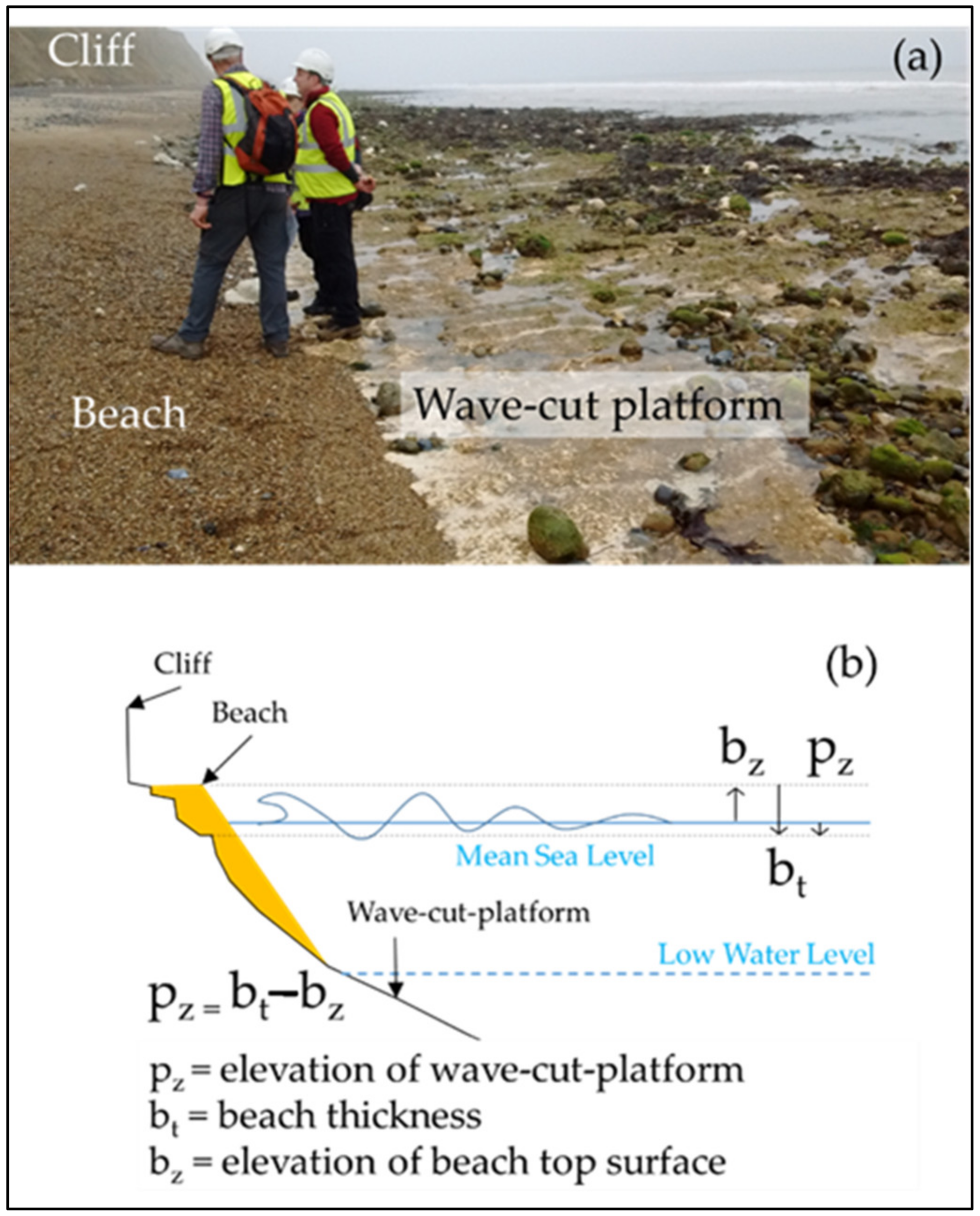
2. Survey Methods and Influence of Beach Environment

2.1. Passive Seismic Survey

Passive seismic surveys measure background seismic noise (both natural <1 Hz and man-made >1 Hz) to estimate the thickness of the different layers through different time domains and spectral techniques. Seismic tremor, commonly called seismic ‘noise’, exists everywhere on the Earth’s surface. It mainly consists of surface waves, which are the elastic waves produced by the constructive interference of P and S waves in the layers near the Earth’s surface. Seismic noise is mostly produced by wind and sea waves. Industries and vehicle traffic also locally generate tremors, although essentially at high frequencies (>1 Hz), which are readily attenuated. Passive seismic surveys consist of a series of single-station point recordings, generally arranged into linear transects. These can be of any length and, when organised into an appropriate grid pattern, can be used to generate 3D surfaces of target horizons. The most reliable results are achieved where independent depth control—such as borehole information—is available to calibrate the results. We used the Tromino ENGY and 3G+ instruments (Tromino/MoHo s.r.l, Venice, Italy), which are small (10 × 14 × 8 cm), portable (~1 kg), broadband, three-component seismometers; and the proprietary software Grilla (v7.0) that implements the horizontal-to-vertical spectral ratio (H/V) method [17,18]. The reason behind using the spectral noise ratio is that seismic noise varies largely in amplitude as a function of the noise ‘strength’ but the spectral ratio remains essentially unaffected and its character is affected by local subsoil structure [19]. The Grilla software also provides routines for quality control of the H/V analyses following the European SESAME project directives [10].

Seismic ground noise acts as an excitation function for the specific resonances of the different layers in the subsoil [20]. For example, if the subsoil has resonant frequencies of 0.8 and 20 Hz, the background seismic noise will excite these frequencies making them visible when applying the H/V technique on the recordings (which are seen as peaks in the ratio of horizontal to vertical components in the seismic spectrum), and these frequencies can be used as a proxy for cover thickness. In a simple double layer stratigraphy comprising sedimentary cover + bedrock, there is a simple equation [21] relating the resonance fundamental frequency f₀ to the thickness h of the layer and Vs (the shear wave velocity in the same layer):

f₀ = Vs/(4h),

(1)

where the value of Vs varies for different materials with typical values of 100–180 m/s for clay, 180–250 m/s for sand, and 250–500 m/s for gravel [22]. In the case of several peaks on the H/V curve, the peak with the lowest frequency is the fundamental mode (f₀, generally the bedrock-cover limit), and other peaks, (i.e., f₁, f₂,…, f_n) correspond to other, shallower geological limits which also cause seismic motion amplification. Based on the expected H/V for all sites, the Tromino was set up to measure background noise for durations of 12 min at 128 Hz sampling frequency. According to the Nyquist frequency [23] the highest frequency that can be recovered from a digitised signal is always lower than half the sampling frequency. Hence, sampling at 128 Hz one can resolve signals at frequencies up to 64 Hz.

The field procedure involved a series of survey locations along two intersecting lines: shore-normal and shore-parallel with (typically) 2 m spacing between readings. At each sampling location, the Tromino instrument was placed directly on the beach surface. When appropriate, a small hole was dug so that it sat below the ground surface to shelter it from the wind. The technique is sensitive to vibration, so activity (movement of people, animals, and machinery) within the immediate vicinity (a radius of about 20 m, [10]) should be kept to a minimum. Processing of the field data involved the following broad steps:

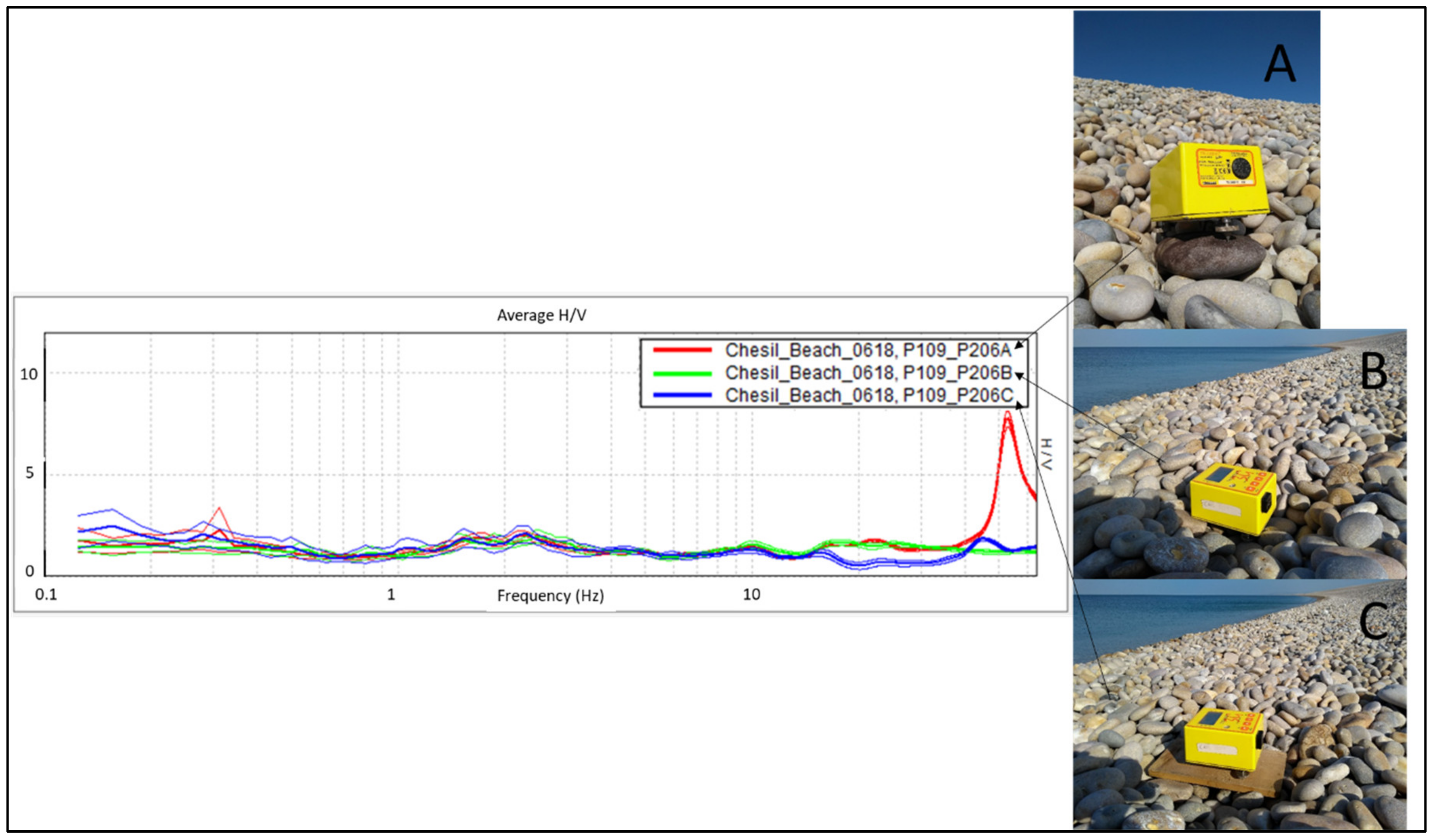
• The raw data gathered at each measurement location were examined, and cleaned by masking out anomalous signals, e.g., caused by activity within the immediate vicinity (~20 m) of the instrument.
• The H/V spectral ratio, as shown in Figure 2 was calculated using the GRILLA software [22]. The fundamental resonance frequencies were identified via interpretation of local maxima with peak values greater than unity on the H/V spectral ratio.
• A velocity function was used to transform the H/V spectral ratio values from the frequency domain into an equivalent spatial domain, i.e., depth. Depending on the information available, this function can range from a single estimate of average velocity to a depth-dependent velocity model. This step was undertaken to map the resonance peak at the frequency identified on the H/V spectrum to a depth equivalent to the base of the layer with the lower acoustic impedance. These H/V-depth files were exported outside of the GRILLA environment and saved in ASCII format.
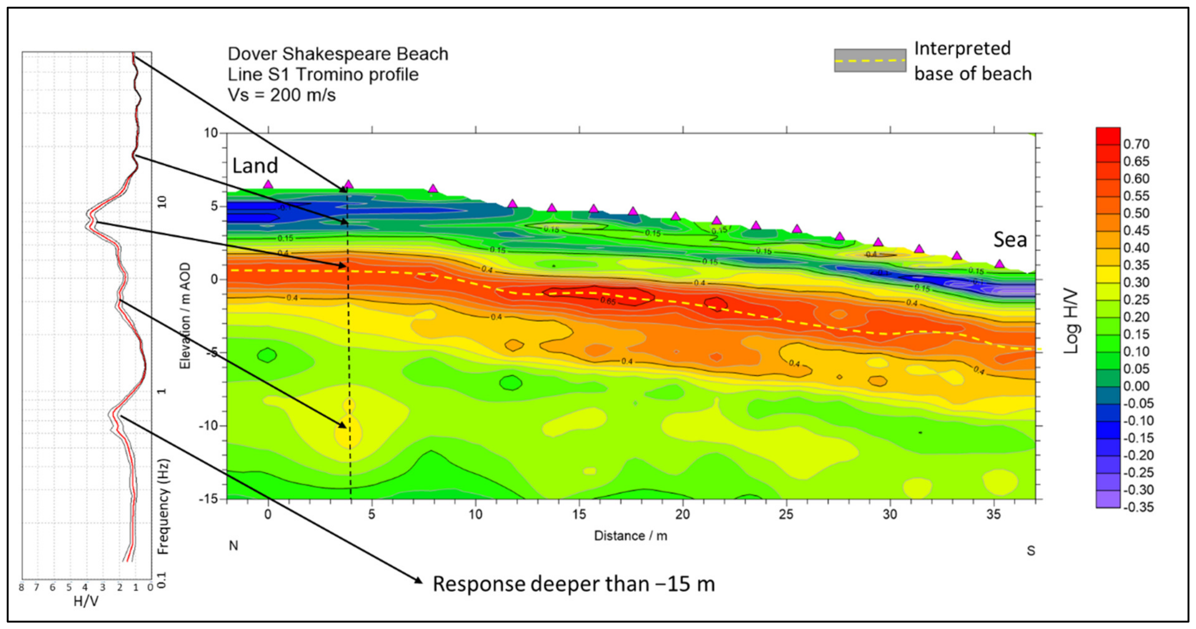
• A 2D section was then constructed via contouring, (using an inverse distance weighted kriging scheme), a series of H/V ratio-depth plots, which were gathered over a succession of survey locations, e.g., along the shore-normal and shore-parallel survey lines; an example of which is shown in Figure 2.

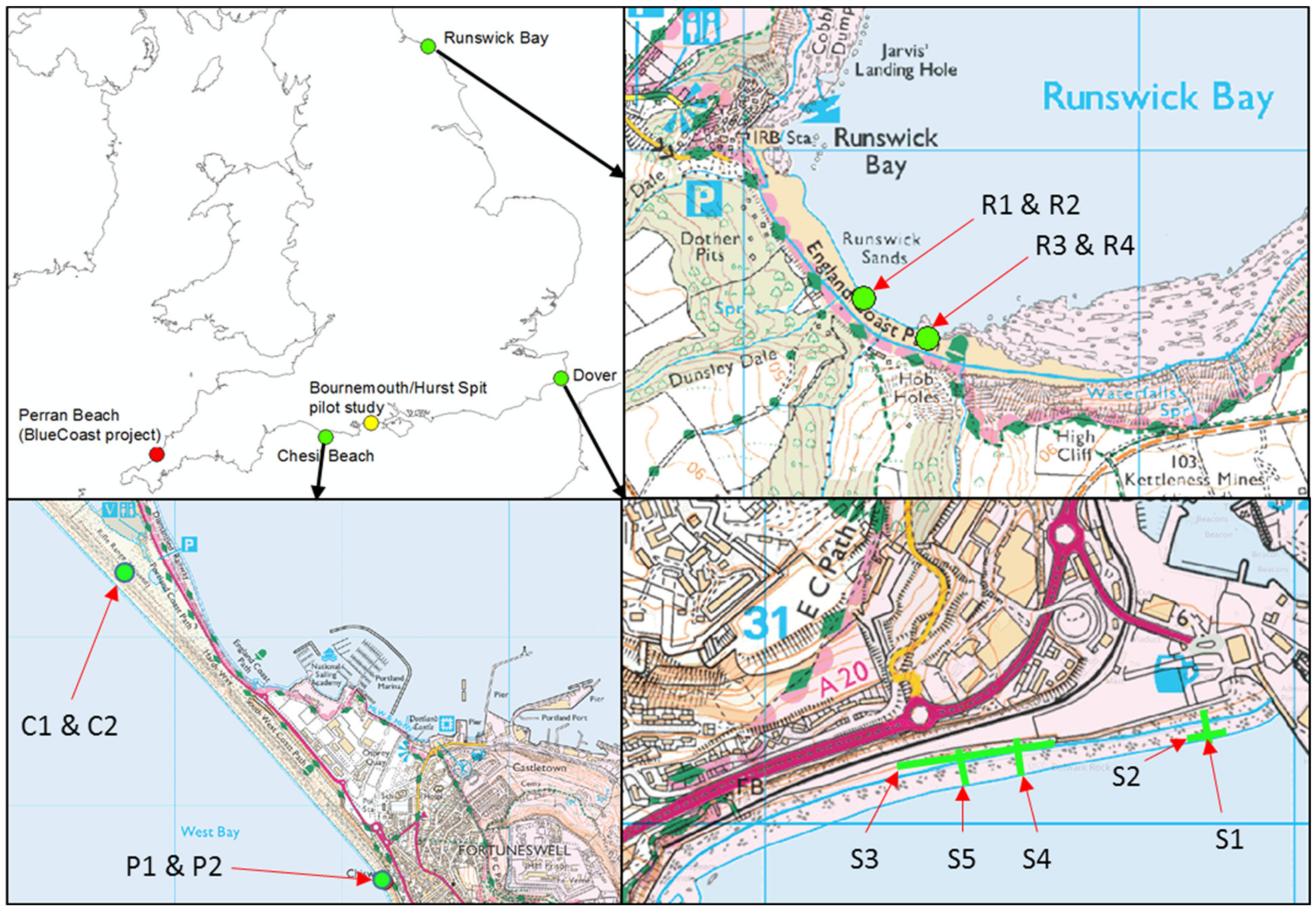
2.2. Study Sites Selection and Description

The methodological performance of the passive seismic technique, including field procedures, instrumental configurations, and settings, was tested at different coastal locations to evaluate its suitability in relation to the following beach characteristics: (1) beach sediment particle size, (2) beach slope angle, and (3) bedrock geology (litho-stratigraphy). Figure 3 shows the locations of the three case study beach sites; the classifications of the beaches are described in

Table 1. Survey itinerary.

	Site Name/Location Chesil	Dover	Runswick
Location	Portland to West Bay, Weymouth, Dorset	Dover Harbour Admiralty Pier to Shakespeare Cliff, Kent	Runswick village to Kettle Ness headland, North Yorkshire
Description	Steep, mostly coarse gravel beach underlain by tidal deposits and Kimmeridge Clay bedrock.	Intermediate to Steep, fine- to medium-gravel beach. Underlying platform: bedrock Chalk.	Low Angle medium to coarse sand with fine to coarse beach overlying glacial till; and Whitby Mudstone Formation bedrock
Phase 1 dates	June 2018	July 2018	August 2018
Phase 1 activity	HVSR; GPS; laser scan.	HVSR; GPS; laser scan; ground-penetrating radar.	HVSR; GPS; laser scan.
Phase 2 dates	February 2019	November 2018	November 2018
Phase 2 activity	HVSR; GPS; laser scan; MASW; seismic monitoring using 24 channels of 3-component geophones in L-array.

. Runswick Bay represented the lowest angle (gradient 0.03; α < 5°), finest grain size, being composed of medium to coarse sand with fine to coarse gravel, underlain by both superficial (glacial till) and weak bedrock comprising Jurassic shale, mudstone, and ironstone of the Whitby Mudstone Formation; Dover represented at an intermediate angle (gradient 0.11–0.17; 5° < α < 10°), fine to medium gravel beach underlain by Chalk bedrock; Chesil represented a high angle (gradient 0.19–0.23; angle α > 10°) coarse gravel to cobble beach underlain by superficial marine deposits and weak Jurassic Kimmeridge Clay bedrock.

Two phases of the survey were undertaken (Table 1). The first phase involved passive seismic surveys for the purpose of evaluating the thickness of beach sediments at each of the three case study sites. These surveys included measurement of beach height and morphology, using differential GPS and terrestrial laser scanning so that assessment and comparison with further surveys were able to account for movement of beach sediment. The second phase involved testing the repeatability of the initial passive seismic surveys, including the sensitivity to orientation of the instrument; recording beach morphology/height to account for changes due to storm activity or replenishment; at Runswick and Dover—an investigation of the modes of seismic propagation contributing to vertical and horizontal vibrations in a beach environment. From these data, a ground model was developed and used to aid the evaluation of the performance of the passive seismic surveys.

3. Results

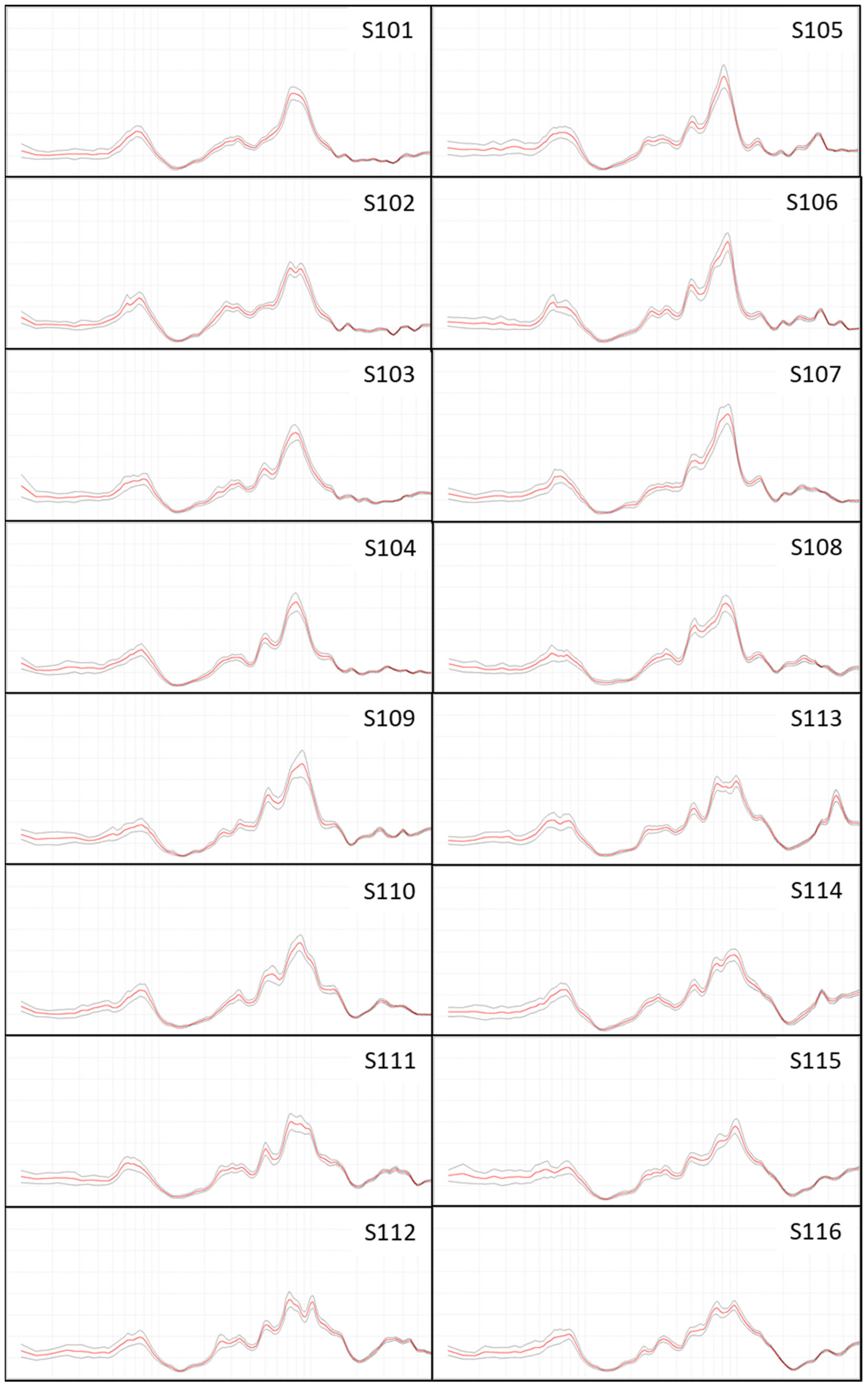
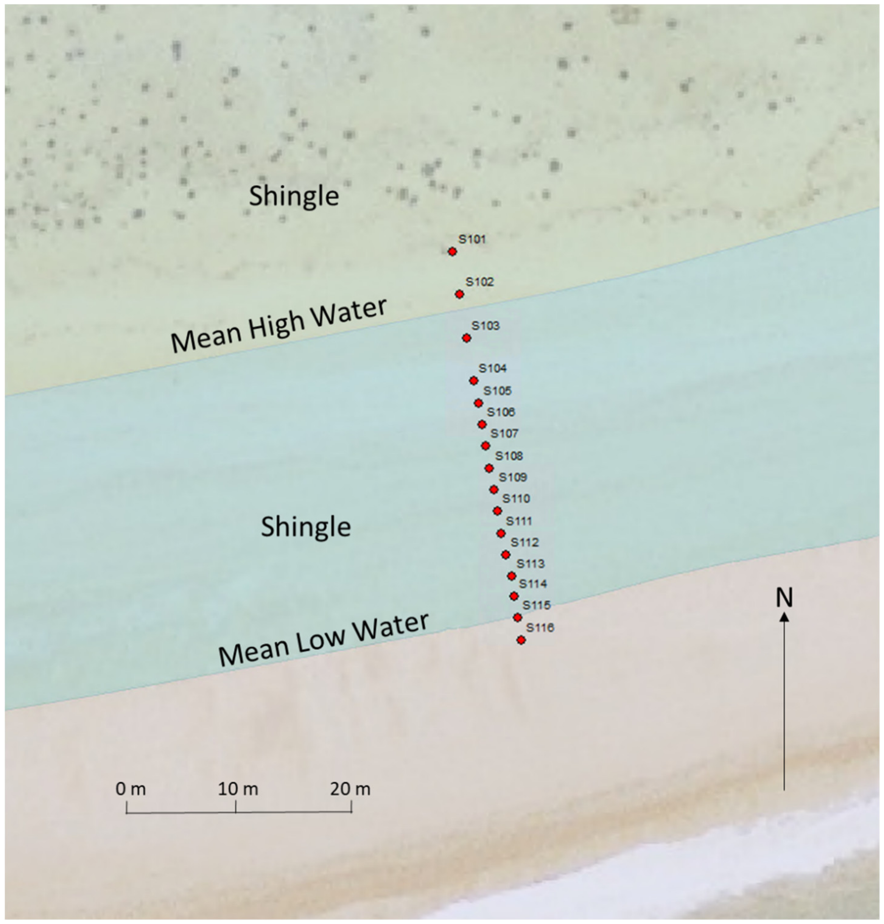
3.1. Field Measurement and Reliability

A series of measurements were undertaken, mounting the Tromino in different ways, as shown in Figure 4. The results show that there are differences in the higher-frequency end of the spectrum, above about 15 Hz, especially a peak at over 50 Hz in the case of mounting on a cobble (which presumably is due to vibration of the cobble). Below 15 Hz all three mounting methods show the same response. It appears that mounting on wood results in a lowering of the H/V ratio between 15 Hz and 40 Hz. While our overall recommendation is to mount the Tromino in the natural sediment, precautions should be undertaken to ensure efficient coupling of the instrument in order to optimise detection of the ground vibration across a broad frequency range. Use of wooden boards or balancing the instrument on large cobbles may involve losses in the coupling either at the base of the instrument or the base of the board or cobble. This in turn will lead to spurious features on the H/V spectra and adversely affect the resulting interpretation.

A sequence of readings was taken at the same locations during the Phase 2 surveys at Runswick Bay and Dover, rotating the instrument through increments of 45°, to see if there are any directional effects on the H/V spectrum. The resulting plots, as shown in Figure 5, show only minor differences across the spectra, indicating that the Tromino response remains consistent as the instrument orientation (azimuth) changes. Generally, the differences between successive spectra fall within the 95% confidence intervals derived from the coherence of the time-slice windows in time–frequency spectrogram.

Reference [10] indicated both low-pressure meteorological events and wind speeds above 5 m/s leading to extraneous perturbations at low frequencies (mainly below 1 Hz) that are not related to site effects. Given that the number of repeat measurements in this study was very small and given the difficulties in quantifying differences in wind and wave conditions between the surveys, it is not possible to separate out their effects on the data. Further research is required to understand the effects of tides, waves, and weather.

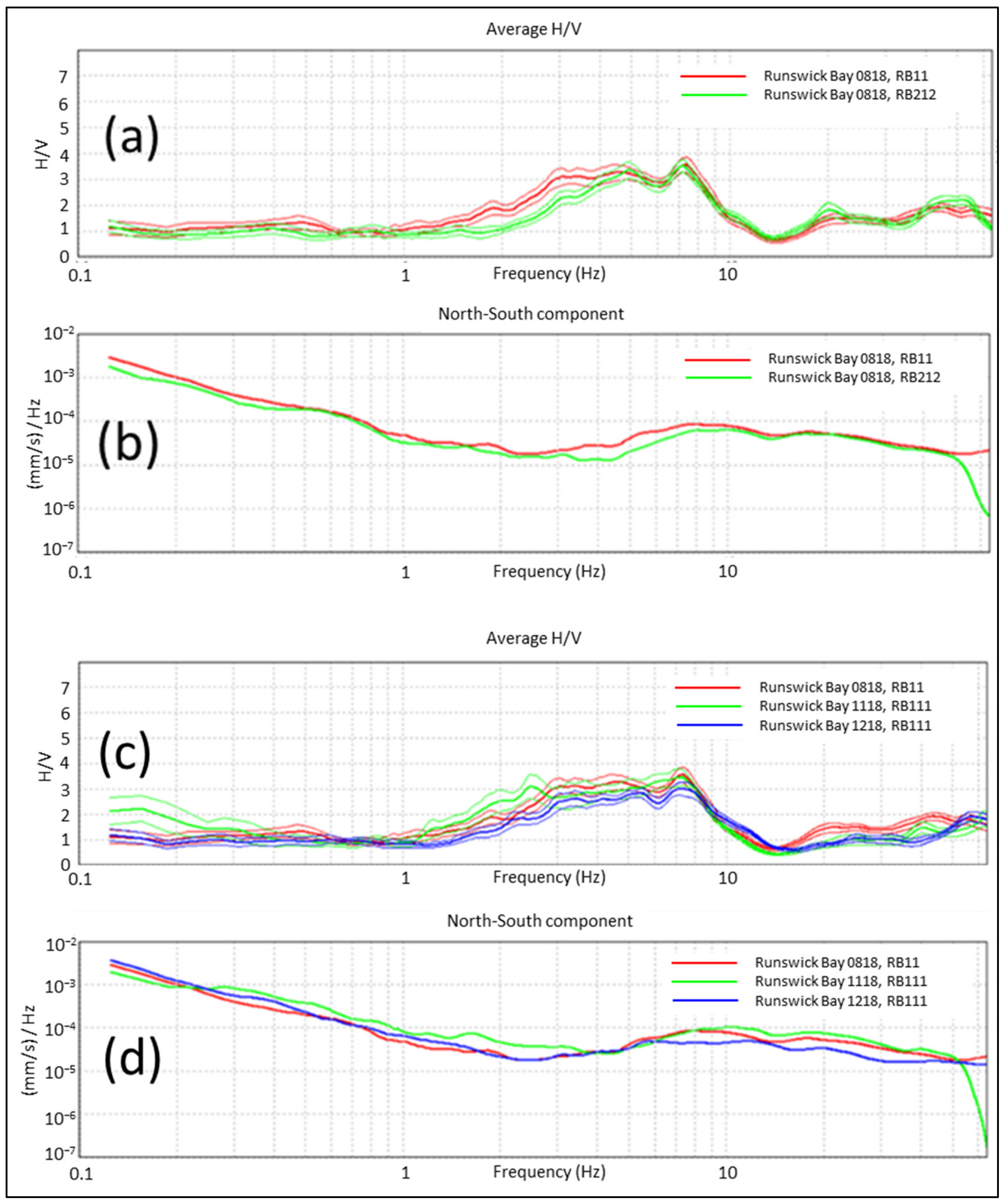
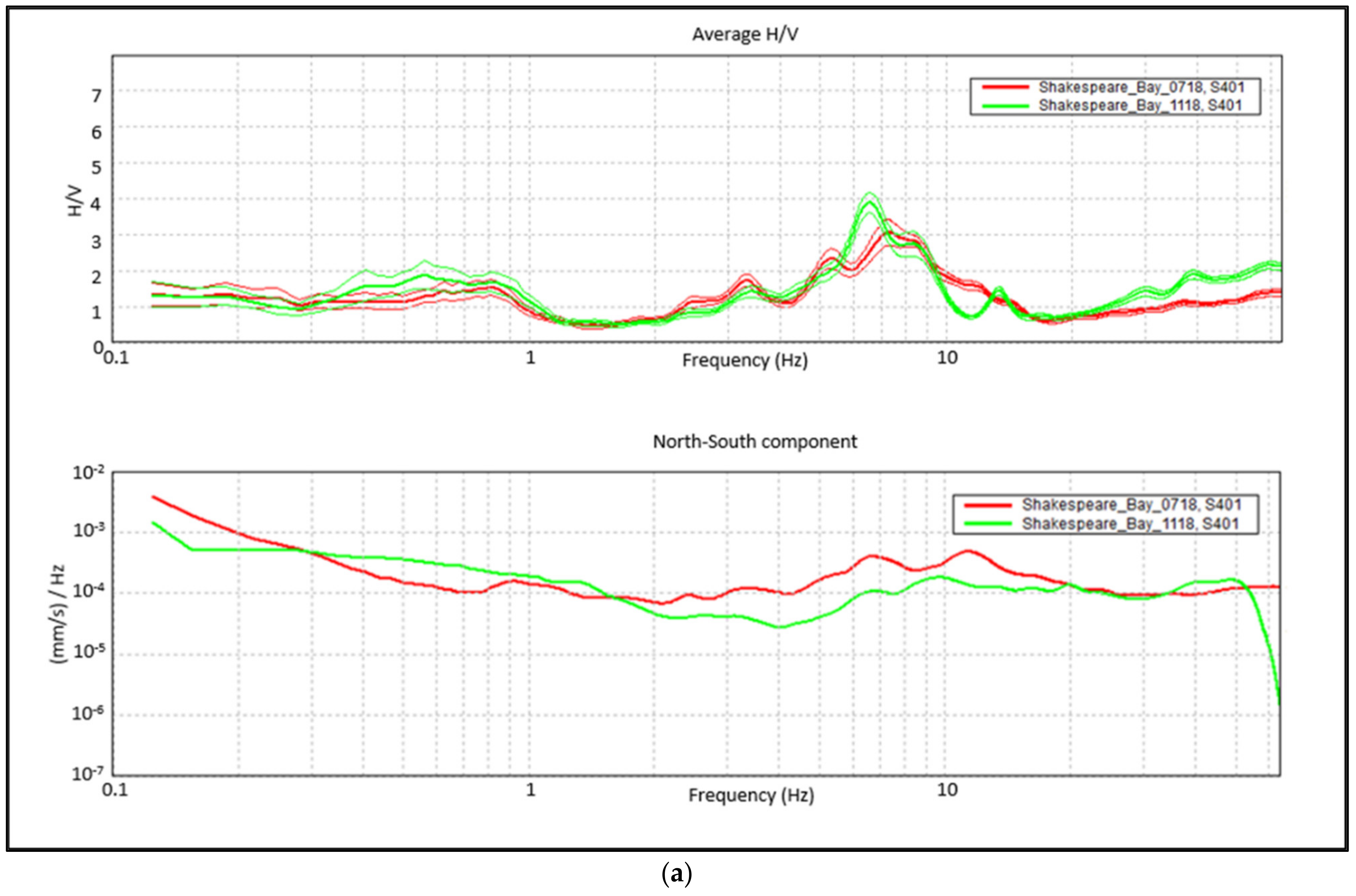
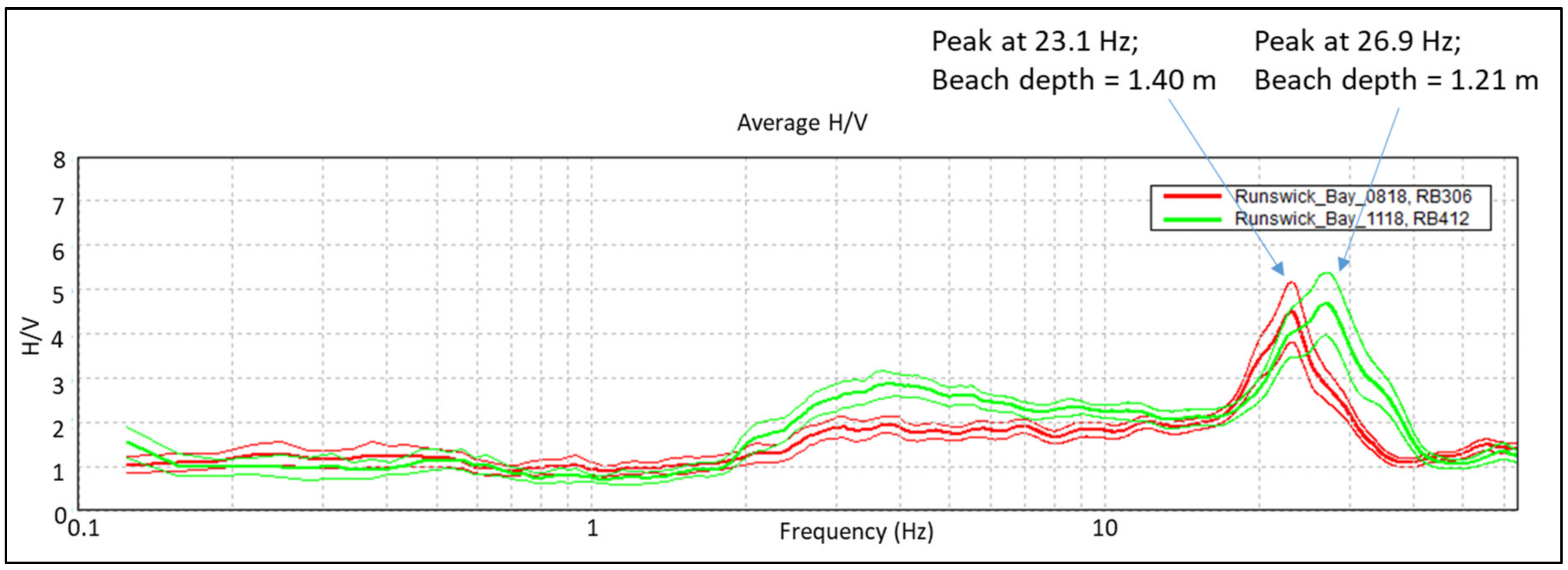
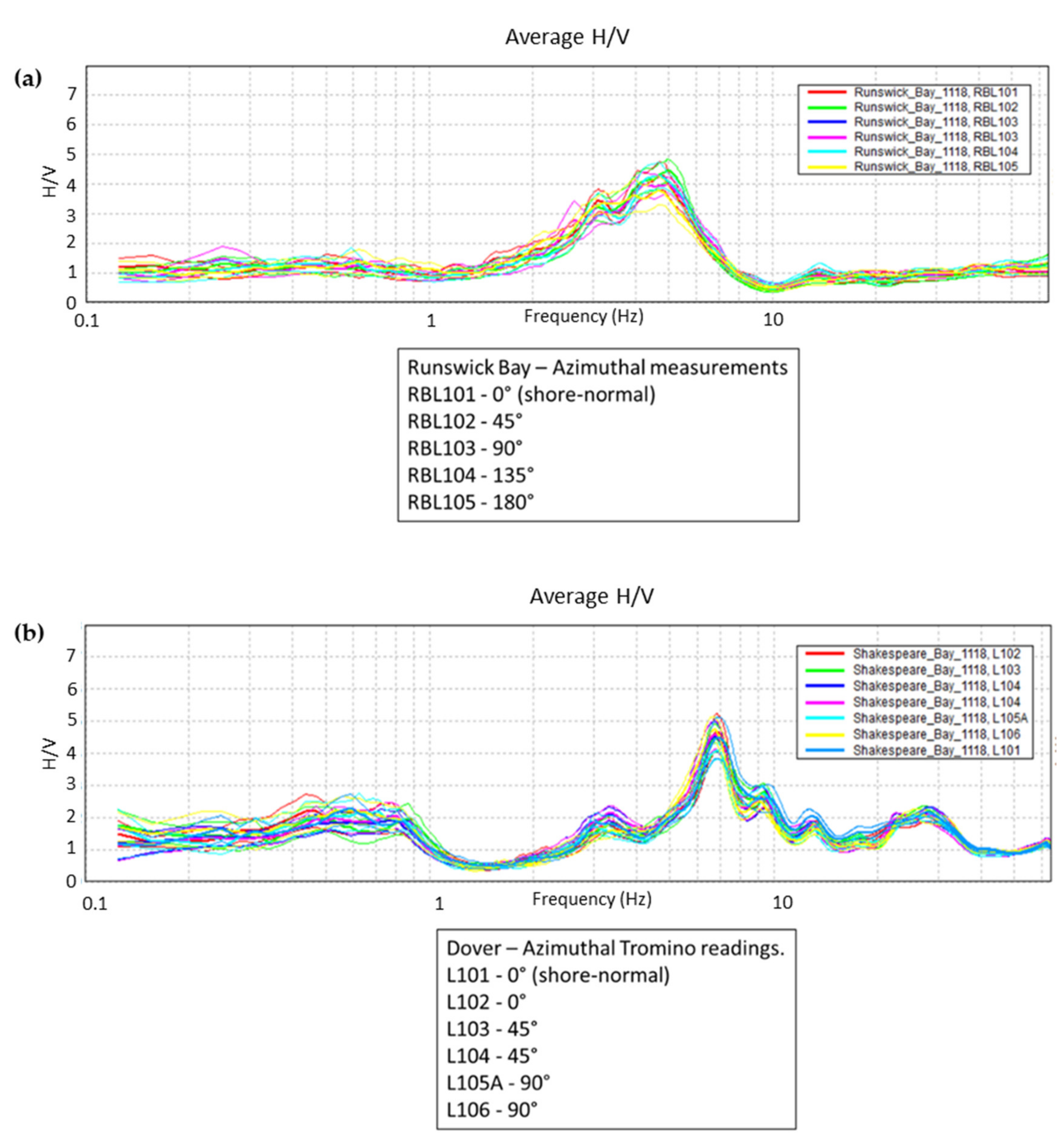
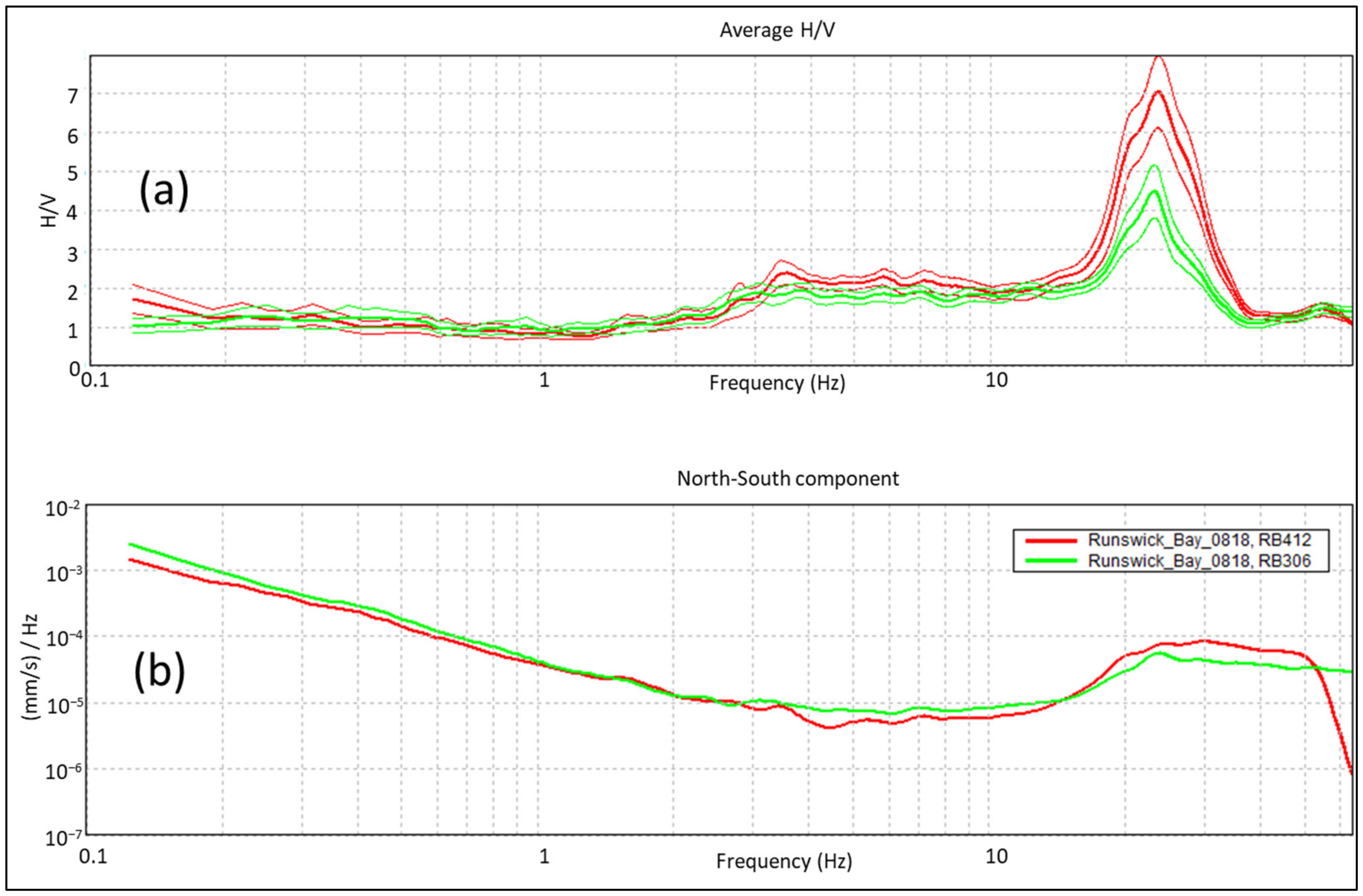
3.2. Variability in Vibrations (within and between Survey Sorties)

Given the dynamic nature of the beach environment, with constantly changing background seismic spectrum due to wind, wave, tidal conditions, and anthropogenic sources, a comparison was made between measurements taken at different intervals in order to see if these had a significant impact on the H/V spectra.

Repeat readings taken on the same day or consecutive days yielded very similar responses. For example, Figure 6a,b from Runswick exhibits small differences in the character of the H/V spectra from measurements taken within 45 min of one another during the August survey between 1 Hz and 4 Hz. In part, these may be related to differences in the horizontal vibration component, which extend from 2 Hz to 9 Hz, and could be due to the ambient wavefield departing from the idealised model that is assumed for HVSR, for instance by localised sources such as anthropogenic activity, or differences in wave action in the sea.

Repeatability between the summer and winter surveys is obviously challenging due to the potential for seasonal changes in the beach profile and composition between and during the successive sorties. Measurements at some locations at Runswick exhibit only minor differences below the peak at 7.5 Hz between the H/V spectra gathered in August, November, and December 2018, Figure 6c,d. (Note that there are also differences in the spectra below 0.4 Hz and above 15 Hz, but neither affect the beach thickness interpretation in this case). Such observations led to the conclusion that there was little change in beach thickness at this locality (calculated to be 1.6 m here), but this was not the case for all locations.

Other examples include differences in the strength of the local peak maxima on successive H/V spectra, as shown in a further example from Runswick in Figure 7. This is due to a stronger horizontal vibration component over a frequency range from 10 to 40 Hz which coincides with the resonance frequency within the beach. Significantly, this change in peak strength does not change the interpretation of the beach thickness (1.2 m at this location).

Significant differences between the summer and winter survey spectra were also observed, on occasion, especially at Dover. A comparison of the H/V spectra at location 1 about profile 4 at Shakespeare Bay reveals a prominent H/V peak at 6.7 Hz in the phase 2 (November) survey but a much more subdued peak of just over 7 Hz in the phase 1 (July) survey, Figure 8a. Similarly, measurements at location 4—profile 4 during the November survey yield H/V spectra with even stronger peaks at 6.7 Hz, Figure 8b. With its proximity to the pier, the road, and the railway, Dover was most affected by traffic and local construction activities, which generally generate frequencies above 1 Hz. The horizontal vibration component was stronger during the July survey than the November survey, which probably relates to differences in the prevailing anthropogenic noise. Pneumatic machinery from a distant source was almost constant during the November survey. The vertical vibration component on the November surveys exhibits fewer fluctuations and a local minimum of 6.7 Hz.

The main H/V peaks as seen in Figure 8 are usually associated with a genuine subsurface structure. By implication, the comparison of surveys indicates the greater presence of extraneous vibrations during the July surveys, which can be investigated by reducing the smoothing (or filtering) of the field data to reveal the raw vibration data. If the smoothing of the spectrum is reduced to 1% (from the default value of 10%), a series of peaks and troughs can be seen in the frequency range of 2 Hz to 50 Hz on the July vibration components, Figure 8b. These are characteristic of man-made activity and note how the noise obscures any dip in the July vertical vibration component leading to an absence of a ‘structural’ peak that is observed in the November survey spectrum.

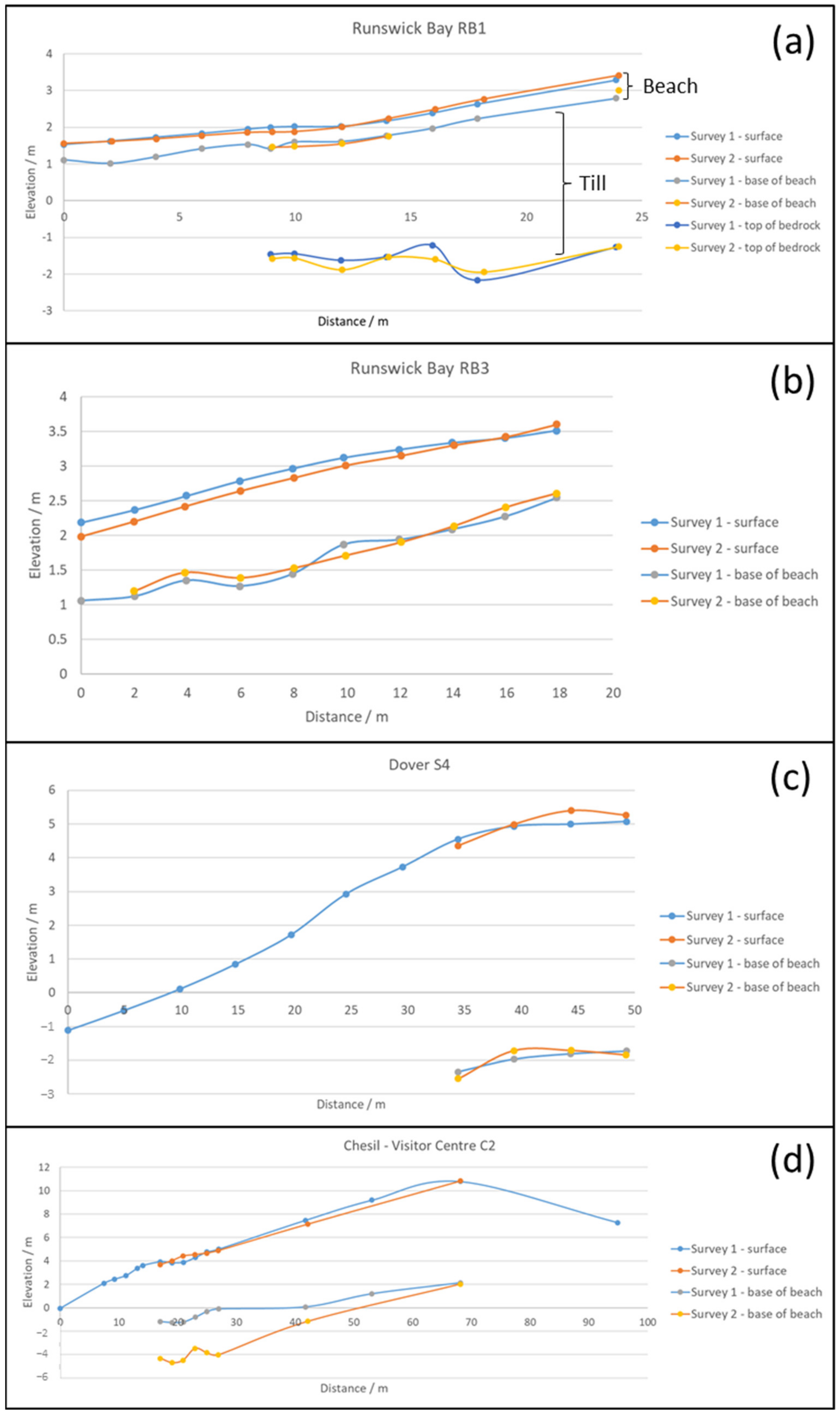
3.3. Effect of Changes in Beach Level (Thickness)

Whilst repeated readings at the same locations on subsequent surveys could potentially show differences due to changes in the beach levels caused by changes in beach sediment thickness, generally, there were only minor changes in beach levels for most of the surveys, which were within the levels of uncertainty of the Tromino data. However, a change in 0.14 m (point elevation measured at 2.97 m AOD in August, and 2.83 m AOD in November) on the thin beach at Runswick Bay provides an illustration of the threshold of detection, beyond which uncertainty falls away enabling us to consider this as a detectable change in beach thickness—see Figure 9.

Using a V_s value of 130 m/s (taken from multi-channel analysis of surface waves (MASW) survey data) and Equation (1) gives:

H = 130/(4f). Where H is the layer thickness.

For f = 23.1 Hz; thickness = 1.40 m

For f = 26.9 Hz; thickness = 1.21 m.

A difference in calculated beach thickness of 0.19 m seems to be an overestimate compared to the change in elevation of 0.14 m measured by the GPS survey, but this is based on shear wave velocities measured at the location of RB1, 200 m away. The discrepancy may reflect the heterogeneity of the beach sediment and/or changes in the sediment between August and November, which would affect the geophysical property profile. Consequently, it is important that passive seismic measurements be accompanied by measurements of shear wave velocity that are representative of the beach sediments and locations tested.

3.4. Repeat Readings: Beach Section Interpretations; Changes between Phases 1 and 2

The phase 2 surveys included revisiting the three study sites and re-siting the Tromino at several of the same locations used in phase 1. While these measurements were made for the purpose of undertaking repeat measurements, it should be noted that at some locations the overall morphology of the beach surface had changed in the time between the survey phases as can be seen in Figure 10. The field data gathered during both phase 1 and 2 were processed in the same manner (as described in this paper) and beach profile contour plots were generated along the same locations for each of the survey phases. This section briefly compares the overall changes between representative profile plots for each study site.

The plots below (Figure 10) show the beach surface for each survey (derived from the GPS data), and the base of the beach taken from an interpretation of the H/V curve for each Tromino measurement. In order to assess the repeatability of the Tromino data, the interpreted base of beach for each survey is shown. If there is no change to the base of the beach and the seismic properties of the beach material remain the same, it should plot in the same position on each survey.

In the case of line RB1, seven repeat readings were undertaken, at the locations along the profile shown in Figure 10a, which includes the points labelled from RB105-RB110, presented in

Table 2. Differences in interpreted beach thickness.

ID	Beach Thickness Survey 1 (m)	Survey1 Base Beach (m OD)	Survey2 Base Beach (m OD)	Base Beach Difference (m)	% Difference (Based on Average Thickness)
Runswick Bay RB1
RB111	0.58	1.419	1.467	−0.048	−10
RB110	0.42	1.597	1.479	0.118	25
RB109	0.42	1.607	1.552	0.055	12
RB108	0.4	1.772	1.758	0.014	3
RB105	0.5	2.785	2.996	−0.211	−45
Average thickness	0.464
Runswick Bay RB3
RB309	1.25	1.122	1.197	−0.075	−6
RB308	1.22	1.352	1.467	−0.115	-9
RB307	1.52	1.268	1.391	−0.123	−10
RB306	1.52	1.447	1.531	−0.084	−7
RB305	1.25	1.873	1.711	0.162	13
RB304	1.3	1.94	1.903	0.037	3
RB303	1.25	2.088	2.134	−0.046	−4
RB302	1.13	2.274	2.404	−0.13	−10
RB301	0.97	2.545	2.605	−0.06	−5
Average thickness	1.27
Dover S4
S404	6.9	−2.347	−2.544	0.197	2.9
S403	6.9	−1.969	−1.713	−0.256	−3.7
S402	6.8	−1.809	−1.708	−0.101	−1.5
S401	6.8	−1.729	−1.84	0.111	1.6
Average thickness	6.85
Chesil C1
C106	5.1	−1.179	−4.321	3.142	54
C107	5.1	−1.264	−4.693	3.429	59
C108	5.1	−1.217	−4.493	3.276	56
C109	5.1	−0.81	−3.468	2.658	46
C110	5.1	−0.338	−3.833	3.495	60
C111	5.1	−0.103	−4.023	3.92	67
C112	7.4	0.069	−1.166	1.235	21
C114	8.65	2.131	2.024	0.107	2
Average thickness	5.83

. The difference in the base of the beach elevation between the repeat measurements ranged between 0.01 m and 0.2 m, but because the beach was thin (on average about 0.5 m), the percentage difference was high (ranging from 3% to 45%). The thin beach also made interpretation of the H/V curve difficult because the peak appears at the highest frequencies. The interpreted depth of the interface between the till (underlying the beach) and the bedrock is also shown in Figure 10. The maximum difference here is 0.4 m over a depth of 4 m (10%); the remaining points all agree to within 0.25 m.

The profile for RB3 (Figure 10b and Table 2) shows a lowering of the beach surface between the two surveys, but the base of the beach is replicated to within 0.162 m (13%), with the majority of measurements showing differences of less than 10%. It is assumed that the beach material has the same acoustic impedance properties on both surveys. (N.B. this paper recommends that future passive seismic surveys include an additional MASW survey to assess the velocity profile through the beach).

The repeat readings for Dover S4 (Figure 10c and Table 2) show differences in the interpreted base of the beach of no more than 0.26 m, and all thicknesses are within 4% of the average. Note that there were issues with anthropogenic noise interfering with measurements at this site, so an extra degree of interpretation was required in identifying the main H/V peak for the base of the beach.

Repeat readings at Chesil Visitor Centre (Figure 10d and Table 2) show major differences in the interpreted beach thickness. The difference appears to increase in the direction towards the sea from the crest of the beach. Difficulties in the base of the beach interpretation related to the low contrast in acoustic impedance between the beach and the underlying geology; differences in the weather and wave conditions on the two surveys which may have led to seismic spectra that did not satisfy the assumptions of the HVSR method; difficulty in obtaining a good coupling of the instrument in the coarse gravel and cobbles of Chesil Beach. The lack of clear results on coarse sediment is discussed below.

4. Discussion of Performance

Anthropogenic sources, such as the movement of people and vehicles, and natural sources, such as sea waves, generate body and surface waves that propagate in the beach and underlying geology. All these modes contribute to horizontal and vertical vibration components that are monitored during passive seismic surveys and can potentially lead to an estimation of the thickness of the beach. The following observations concerning the overall beach model and underlying geology were made at each of the sites:

Runswick: A beach predominantly comprising gravelly sand overlying a very shallow sloping, foreshore platform of either glacial till or Whitby Mudstone. Certainty in this ground model interpretation is high due to the thin cover from the beach and the accessibility of the underlying geology via visual observation and invasive sampling, such as cone penetration resistance test (CPT). Weaker, lower amplitude resonance peaks were recorded from surveys over the glacial till compared to over the Whitby Mudstone. This has been attributed to a lower acoustic impedance contrast between the beach and the till relative to that between the beach and the mudstone. Consequently, while a continuous interface between the beach and the mudstone could be interpreted, the interface between the beach and the till was discontinuous. Hence, misinterpretation of the beach thickness is possible at locations where resonance peaks at the appropriate frequencies are absent from the passive surveys. Potentially, the Runswick site tested the limit of the Tromino capability in relation to: (i) very low contrast in the acoustic impedances of the beach and the underlying glacial till, i.e., the peak H/V spectral ratios measured over the till were less than 2; (ii) the low beach thickness resulted in resonance peaks at frequencies greater than 10 Hz, i.e., within frequency bands where much anthropogenic noise is generated.

Dover: A beach predominantly comprising coarse sand, and fine to medium gravel overlying a Chalk foreshore platform. Again, certainty in this ground model is high due to visual observations of the chalk platform after previous storm events that led to the replenishment of the beach sediments and rock armour to protect the railway. Large amplitude resonance peaks were recorded from the surveys at Dover, which have been attributed to a strong acoustic impedance contrast between the beach and the underlying chalk. Thus, a continuous interface between the beach and underlying chalk could be interpreted. Dover presented a case study site where the Tromino was very effective. Dover Shakespeare Beach comprised sediments with: (i) a strong acoustic impedance contrast with the underlying platform geology, resulting in H/V spectral ratios much greater than 2, and (ii) a sediment thickness of greater than 3 m resulting in resonance peaks at frequencies below 10 Hz.

Chesil: A barrier beach predominantly comprising medium to coarse gravel overlying mixed silt, sand, and gravel believed to have been deposited in a tidal lagoon or estuarine environment. Certainty in this ground model is highest around the back-shore zone by the Chesil Visitor Centre where the underlying geology was observed and sampled with invasive CPT. However, high sea levels prevented any visual inspection of the geology underlying the beach in the foreshore zone. The geology underlying the beach may include marine sediments of low density. Very low acoustic impedance contrasts between the beach and the underlying sediments led to H/V spectral ratios of less than 2, and subsequently, the base of the beach was difficult to interpret. Difficulties were encountered in seating the Tromino instrument on the beach at the Chesil Portland site. It is suspected that difficulties in obtaining satisfactory seating on beaches grading between very coarse gravels and cobbles lead to poor coupling between the instrument and the ground vibrations. Poor coupling resulted in a potential loss in vibrations, which we suspect were frequency-dependent, resulting in missing bands in the H/V spectrum. While particle size exerts primary control over the foreshore slope, where gravel (shingle) beaches are steeper than sand beaches [24,25,26], the degree of exposure, and erosional vs accretionary processes also influence beach slope angle. Hence, beach angles encountered at the study sites did not have a direct effect on the performance of the passive seismic instrument. However, it cannot be discounted that because of the association between particle size and beach angle, the reliability of the passive seismic technique decreases with increasing beach angles.

In addition to the comments made above about each of the beaches in this study, temporal changes in the underlying beach conditions will influence the determination of the depth to bedrock. The most significant of these include changes in the thickness of the beach sediments and how their geophysical property profile contrasts with the underlying strata. The beach thickness (and hence height) changes in response to phases of erosion or replenishment associated with natural or anthropogenic processes.

The geophysical property profiles—especially the shear wave velocity profile, are affected by beach sediment type, proportion, and distribution within the beach profile and effective stress conditions, which are themselves, affected by the beach packing density, tidal height, and the hydrostatic levels/pressures within the beach profile. Changes in the geophysical property profiles are difficult to quantify comprehensively using non-invasive methods. However, changes in the shear wave property profile can be monitored, which can be done by undertaking a multi-channel analysis of surface waves during site visits (see Appendix A for more details).

A change in beach height is detected by the passive seismic beach thickness determination, as illustrated in Part 3.3. This led to our recommendation that passive seismic surveys are accompanied by beach height surveys, as well as representative velocity surveys.

5. Conclusions

When a beach is present, there is always underneath a wave-cut platform or a layer of different mechanical properties than the beach loose deposits. If this layer of transportable sediment is relatively thin, it can accelerate the abrasion of the platform underneath and if it is thick enough will protect the shore from abrasion [7]. The presence of the wave-cut platform has a direct effect on shoreline evolution via the sediment budget contribution but also indirectly via affecting the alongshore sediment transport gradient. Passive seismic survey (PSS) based on the HVSR technique is a promising, portable non-intrusive technique that could be potentially used to measure beach thickness but the suitability of the technique from previous studies remains inconclusive [9,15] due to impedance contrast between the wave-cut platform and beach deposits not high enough to use this technique. The suitability of PSS to estimate beach thickness in other geological coastal environments was largely unexplored before this study where we have tested the methodological performance of the PSS technique, including field procedures, instrumental configurations, and settings, at different coastal locations to evaluate its suitability in relation to the following beach characteristics: (1) beach sediment particle size, (2) beach slope angle, and (3) bedrock geology (litho-stratigraphy). The performance of the technique is summarised in detail in the previous section and the main highlights are described here.

The results show that the HVSR technique is a suitable tool for assessing the thickness of beach sediments composed of sand to medium gravel. The Tromino instrument used in this study has the advantage over other geophysical techniques of being small, lightweight, and easy to deploy without causing disturbance to the beach environment or obstructing beach users. The instrument produced consistent, repeatable results under a range of conditions: weather; state of the tide; minor changes in beach geomorphology; azimuthal orientation of the instrument.

The instrumental performance is affected by the survey set-up and standard procedures are recommended below to ensure optimal and consistent field records. Certain conditions in some beach environments can compromise these set-up standards and lead to a deterioration in the survey performance. For example, these conditions include poor seating of the instrument on very coarse beach sediments or high winds generating a lot of noise. Hence, limitations on the environmental conditions in which the Tromino should be used are advised in Appendix A.

The instrument performs best where there is a large acoustic impedance contrast between the beach sediments and underlying geology. This is most likely to occur where the beach is underlain by competent bedrock. Performance deteriorates with decreasing acoustic impedance contrast between the beach and underlying geology. For example, poor survey performance is anticipated where the geology underlying the beach is of comparable acoustic impedance to that of the beach above. This is most likely to occur where the beach is underlain by weak superficial geology.

The method is able to detect changes in beach thickness of the order of 15 cm when compared with the change in elevation measured by a GPS survey. It is important that passive seismic measurements be accompanied by measurements of shear wave velocity that are representative of the beach sediments and locations tested. Alternatively, for places where there is a large number of independent beach thickness values, these could be combined with peak frequency measurements [27] to construct an empirical relationship between them avoiding the need to measure the shear velocity.

References

1. Bowen, A.J.; Inman, D.L. Budget of Littoral Sands in the Vicinity of Point Arguello, California; US Department of the Army, Corps of Engineers: Washington, DC, USA, 1966. [Google Scholar]
2. Rosati, J.D. Concepts in sediment budgets. J. Coast. Res. 2005, 21, 307–322. [Google Scholar] [CrossRef]
3. Cooper, N.; Pontee, N. Appraisal and evolution of the littoral ‘sediment cell’concept in applied coastal management: Experiences from England and Wales. Ocean Coast. Manag. 2006, 49, 498–510. [Google Scholar] [CrossRef]
4. Hinton, C.; Nicholls, R.J. Spatial and temportal behavior of depth of closure along the holland coast. Coast. Eng. Proc. 1998, 1999, 2913–2925. [Google Scholar]
5. Nicholls, R.J.; Birkemeier, W.A.; Lee, G.-H. Evaluation of depth of closure using data from Duck, NC, USA. Mar. Geol. 1998, 148, 179–201. [Google Scholar] [CrossRef]
6. López, P.M.; Payo, A.; Ellis, M.A.; Criado-Aldeanueva, F.; Jenkins, G.O. A Method to Extract Measurable Indicators of Coastal Cliff Erosion from Topographical Cliff and Beach Profiles: Application to North Norfolk and Suffolk, East England, UK. J. Mar. Sci. Eng. 2020, 8, 20. [Google Scholar] [CrossRef] [Green Version]
7. Payo, A.; Hall, J.W.; Dickson, M.E.; Walkden, M. Feedback structure of cliff and shore platform morphodynamics. J. Coast. Conserv. 2014, 18, 847–859. [Google Scholar] [CrossRef] [Green Version]
8. Kobayashi, N.; Zhu, T. Erosion by wave action of consolidated cohesive bottom containing cohesionless sediment. J. Waterw. Port Coast. Ocean Eng. 2020, 146, 04019041. [Google Scholar] [CrossRef]
9. Payo, A.; Walkden, M.; Ellis, M.; Barkwith, A.; Favis-Mortlock, D.; Kessler, H.; Wood, B.; Burke, H.; Lee, J. A quantitative assessment of the annual contribution of platform downwearing to beach sediment budget: Happisburgh, England, UK. J. Mar. Sci. Eng. 2018, 6, 113. [Google Scholar] [CrossRef] [Green Version]
10. Sesame, W. Guidelines for the Implementation of the H/V Spectral Ratio Technique on Ambient Vibrations-Measurements, Processing and Interpretation; SESAME European Research Project, Deliverable D23.12, Project No. EVG1-CT-2000-00026 SESAME; European Commission: Brussels, Belgium, 2004; 62p. [Google Scholar]
11. Nogoshi, M. On the amplitude characteristics of microtremor, Part II. J. Seismol. Soc. Jpn. 1971, 24, 26–40. [Google Scholar]
12. Nakamura, Y.; Saito, A. Estimations of amplification characteristics of surface ground and PGA using strong motion records. Proc. 17th JSCE Earthq. Eng. Symp. 1983, 17, 25–28. [Google Scholar]
13. Nakamura, Y. A method for dynamic characteristics estimation of subsurface using microtremor on the ground surface. Railw. Tech. Res. Inst. Q. Rep. 1989, 30, 25–33. [Google Scholar]
14. Raines, M.G.; Gunn, D.A.; Morgan, D.J.R.; Williams, G.A.; Caunt, S. Refraction microtremor (ReMi) to determine the shear-wave velocity structure of the near surface and its application to aid detection of a backfilled mineshaft. Q. J. Eng. Geol. Hydrogeol. 2011, 44, 211–220. [Google Scholar] [CrossRef]
15. Gunn, D.; Pearson, S.; Chambers, J.; Nelder, L.; Lee, J.; Beamish, D.; Busby, J.; Tinsley, R.; Tinsley, W. An evaluation of combined geophysical and geotechnical methods to characterize beach thickness. Q. J. Eng. Geol. Hydrogeol. 2006, 39, 339–355. [Google Scholar] [CrossRef] [Green Version]
16. Payo, A.; Jenkins, G.O.; Morgan, D.; Valiente, N.G.; Scott, T. Evidence of Former Sea Levels from a Passive Seismic Survey at a Sandy Beach; Perranporth, SW England, UK. J. Mar. Sci. Eng. 2022, 10, 569. [Google Scholar] [CrossRef]
17. Aki, K.; Richards, P.G. Quantitative Seismology; University Science Books: Sausalito, CA, USA, 2002. [Google Scholar]
18. Ari, B.-M.; Singh, S.J. Seismic Waves and Sources; Springer Science & Business Media: New York, NY, USA, 1981. [Google Scholar]
19. Guillier, B.; Chatelain, J.-L.; Bonnefoy-Claudet, S.; Haghshenas, E. Use of Ambient Noise: From Spectral Amplitude Variability to H/V Stability. J. Earthq. Eng. 2007, 11, 925–942. [Google Scholar] [CrossRef]
20. Moho. Tromino User’s Manual; Moho Science and Technology: Venice, Italy, 2017. [Google Scholar]
21. Bonnefoy-Claudet, S.; Köhler, A.; Cornou, C.; Wathelet, M.; Bard, P.-Y. Effects of Love waves on microtremor H/V ratio. Bull. Seismol. Soc. Am. 2008, 98, 288–300. [Google Scholar] [CrossRef]
22. Micromed. Introduction to the H/V Modelling Routine for Stratigraphic Purposes in Grilla; Micromed s.p.a.: Treviso, Italy, 2012. [Google Scholar]
23. Shannon, C.E. Communication in the presence of noise. Proc. IRE 1949, 37, 10–21. [Google Scholar] [CrossRef]
24. Wiegel, R. Oceanographical Engineering; 95–127, Tsunamis, Storm Surges, and Harbor Oscillations; Dover Publications: Mineola, NY, USA, 1964. [Google Scholar]
25. Komar, P.D. Beach processes and sedimentation. Eos 1998, 79, 231. [Google Scholar]
26. Leadon, M. Beach slope and sediment-grain-size trends as a basis for input parameters for the SBEACH erosion model. J. Coast. Res. 2015, 31, 1375–1388. [Google Scholar] [CrossRef]
27. Guo, Z.; Aydin, A.; Huang, Y.; Xue, M. Polarization characteristics of Rayleigh waves to improve seismic site effects analysis by HVSR method. Eng. Geol. 2021, 292, 106274. [Google Scholar] [CrossRef]
Figure 1. Wave-cut platforms are often covered by beach deposits and their position can be obtained from beach thickness and beach elevation: (a) photo taken near Trimingham, East England showing a cliff, beach, and wave-cut platform (source BGS); (b) schematic showing how wave-cut platform can be obtained from beach thickness and elevation observation.
Jmse 10 00667 g001
Figure 2. Colour contour 2D profile (right) derived from the results of a number of H/V measurements and an individual H/V spectrum from a single measurement (left), showing how the H/V peaks and troughs relate to the colour contour plot. Magenta triangles show the location of Tromino measurements along the profile. The profile location is shown in Figure 3 and Figure A2.
Jmse 10 00667 g002
Figure 3. Overview map of the sites surveyed as part of the project (in green), and other related studies in yellow and red. Contains Ordnance Survey data © Crown copyright and database rights 2022 Ordnance Survey Licence No. 100021290 EUL.
Jmse 10 00667 g003
Figure 4. Three readings taken at Chiswell, showing the effect of different mounting. (A)—on a single flat cobble; (B)—directly on beach sediment; (C)—on a piece of wood.
Jmse 10 00667 g004
Figure 5. Plot of azimuthal readings at (a) Runswick Bay and (b) Dover, showing the results of readings taken at 45° intervals. The similarity of the traces shows the lack of directional influence of the ambient wavefield. All measurements taken within a period of 30 min and at an intermediate state of tide.
Jmse 10 00667 g005
Figure 6. (a,b): Repeat readings, Runswick Bay Phase 1; showing some differences in the H/V ratio between 1.5 Hz and 4 Hz, which may be related to differences in the horizontal vibration component. (a) Shows the average H/V and (b) the North–South component. (c,d): Repeat readings, Runswick Bay: August, November, and December, showing similar responses between 1 Hz and 10 Hz, and differences above 15 Hz—perhaps a result of changes in the beach sediment.
Jmse 10 00667 g006
Figure 7. Repeat readings, Runswick Bay Phase 1; a good example of the amplitude of the H/V peak changing, whilst the frequency remains the same. (a) Shows the average H/V and (b) the North–South component. Measurements were taken approximately 90 min apart, using different instruments.
Jmse 10 00667 g007
Figure 8. Contrasting readings taken at the same location at Dover, showing differences in the spectrum, attributed to anthropogenic sources of seismic energy. (a) Profile 4, location 1. (b) Profile 4, location 4.
Jmse 10 00667 g008aJmse 10 00667 g008b
Figure 9. Measurements taken at the same location in August 2018 and November 2018, illustrating the effect of a change in beach thickness.
Jmse 10 00667 g009
Figure 10. Plot of beach surfaces (from GPS) and interpreted base of beach for (a) line RB1, Runswick Bay; (b) line RB3, Runswick Bay; (c) line S4, Dover; (d) line C2, Chesil Visitor Centre.
Jmse 10 00667 g010