Abstract
As international regulations on greenhouse gas emissions are becoming stricter, the development of eco-friendly main engines is required for ocean-going ships. To use cryogenic LNG as a fuel for marine engines, it has to be converted to gas. This processing device is called an LNG regasification system. This paper presents a DS-based PID controller for glycol temperature control of a regasification system for LNG-fueled marine engines. In controller design, linear PID controllers have something of a catch-22 relationship: Fast response requires a large gain, which results in a large overshoot. To solve this problem, a DS-based 2-DOF PID controller is considered, which consists of a PID controller to reject disturbances in regulatory response and a set-point filter to reduce overshoot in servo response. The controller design focuses on improving disturbance rejection performance. The DS method is based on comparing the desired closed-loop characteristic equation with the closed-loop characteristic equation consisting of a control object and PID controller. The proposed controller is applied to the glycol temperature control of the regasification system for LNG-fuel marine engines, and its performance is compared with existing methods to show its effectiveness and applicability.
1. Introduction
In accordance with Appendix VI of 1997 MARPOL Protocol [1], the International Maritime Organization (IMO) has issued regulations for reducing emissions of air pollutants such as sulfur oxides (SOx), nitrogen oxides (NOx), carbon dioxide (CO2), and from marine vessels.
As the IMO enforces significantly tightened emission limits, one of the solutions for reducing emissions is the use of an eco-friendly fuel, liquefied natural gas (LNG). Compared to heavy oil, LNG generates only 75% of CO2, 10% of NOx, and 5% of SOx. Meanwhile, some engine manufacturers have developed LNG-fueled marine engines [2,3]. Using LNG as a fuel for engines requires special equipment that can handle cryogenic temperatures (−163 °C). In order to use LNG as a fuel, it must be changed to a gaseous state at about 30–45 °C. This processing device is called an LNG regasification system, which consists of a heat exchanger, a regulating valve, and a controller. To control glycol temperatures in a heat exchanger system, it is necessary to model the equipment such as the heat exchanger and regulating valve, etc. However, since heat exchangers have nonlinearity, there are limitations in obtaining an accurate model. Moreover, since its parameters may change during operation, some fixed-gain controllers are effective in limited operating ranges, but deviations from them can degrade performance and lead to them becoming unstable [4]. Moreover, since large heat exchangers take a lot of time to transfer heat, it is difficult to control the temperature to ensure stable performance, so many studies have been conducted to improve this problem. Choi [5] added a feedforward controller to the existing PID (proportional–integral–derivative) controller to reduce the change in coolant temperature due to load variation in the main engine. Ahn et al. [6] proposed a double-loop cascade control system for controlling the temperature of the main engine jacket coolant to alleviate the sudden temperature changes caused by disturbances. Vasičkaninová et al. [7], and Oravec et al. [8] proposed a discrete model predictive control algorithm. Duka et al. [9], Beirami et al. [10], Kumar et al. [11], and Emhemed et al. [12] suggested a method for combining PID controllers using fuzzy control. Padhee et al. [13,14,15], Khanvilkar et al. [16], and Sarabeevi et al. [17] addressed issues related to PID controllers based on internal model methods. Manikandan et al. [18], Skorospeshkin et al. [19], and Xiao et al. [20] proposed a controller based on adaptive control.
In model-based controller design, it is very important to select the appropriate mathematical model for the plant. If the correct model for the plant to be controlled is not selected, satisfactory control performance cannot be expected, no matter how well the parameters of the controller are tuned. First order plus time delay (FOPTD) models have been widely used in controller design because most of the industrial processes are over-damped stable systems with time delay. Industrial heat exchanger systems can be approximated to some extent by FOPTD models. In particular, FOPTD models make it difficult to design controllers with satisfactory control performance due to time delay, which is a nonlinear factor. Many methods for designing and tuning PID controllers have been reported for FOPTD models. These are the optimization method [21,22], internal model control method [23,24,25], direct synthesis method [26,27,28] and nonlinear control method [29,30], etc. Tavakoli [21] reported a method for tuning the PID controller for FOPTD models using optimization techniques and used integrals related to errors as evaluation indices. Jin et al. [22] proposed three tuning rules for a simple nonlinear PID controller for an FOPTD model. The proposed controller is based on the structure of an ideal parallel type PID controller. The optimal parameters of the proposed PID controller for the set-point input are tuned with a genetic algorithm (GA) after performing dimensional analysis. Simulations performed on higher-order processes provided better performance than the linear PID controller of Tavakoli. Lee et al. [24] revisited the SIMC (Skogestad’s internal model control) method of Skogestad [23] and proposed a new method (K-SIMC) for tuning the PID controller. In this method, Skogestad’s approximation method has been slightly modified, and new tuning rules have been proposed that limit the integral time much more than Skogestad’s method, and a set-point filter added that was not used in Skogestad’s method.
Anil et al. [27] proposed a PID controller design technique for controlling various types of models with time delays using a direct synthesis method, but FOPTD models were not included. Thus, [31] proposed a modified 2-DOF (two degree of freedom) control, and covered how to optimally tune the parameters of a PID controller. The set-point weighted PID controller was implemented by combining a feedforward controller and a PID controller within a framework, and the parameters of the proposed controller were optimally tuned using a GA in view of minimizing the integral of absolute error.
In this paper, a 2-DOF PID controller based on a direct synthesis is proposed to simultaneously improve the set-point tracking and disturbance rejection response on glycol temperature control of a regasification system for LNG-fueled marine engines, and the PID parameter tuning method is discussed. The 2-DOF PID controller consists of a PID controller for rejecting the disturbance in regulatory response and a set-point filter for reducing the overshoot in servo response, and the controller design focuses on improving input disturbance rejection performance. The proposed controller is compared with existing methods to show its effectiveness and applicability.
The composition of this paper is as follows: Section 2 explains the structure of the regasification system and the modeling of each element. Section 3 deals with the design method of the proposed 2-DOF PID controller consisting of a PID controller for disturbance rejection based on the DS technique and a set-point filter for set-point tracking. Section 4 describes the PID parameter tuning method. Section 5 applies the proposed method to temperature control of the regasification system of an LNG-fueled marine engine, and its performance is compared with the conventional PID controllers. Conclusions are drawn at the end.
2. Structure of Regasification System and Modelling
In order to supply LNG as a fuel to marine engines, a regasification system is needed to raise it to the appropriate temperature and convert it into gas. Figure 1 shows an example of a regasification system for an LNG-fueled marine engine.
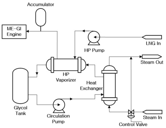
Figure 1.
A regasification system for LNG-fueled marine engine.
The regasification system consists of the primary and secondary loops. The cryogenic LNG in the primary loop is boosted by the HP pump to approximately 250 to 300 (bar) converted into a gaseous state of about 35 to 45 °C while passing through an HP vaporizer, and fed into the marine engine cylinder via an injector. At this time, heat is supplied to the LNG from the glycol. On the other hand, the glycol cooled in the HP vaporizer in the secondary loop needs to be reheated by the hot steam supplied to the heat exchanger. The heat exchanger used in the regasification system is a shell and tube type, and the flow type is counter flow with several passes. In summary, heat exchange occurs between LNG and glycol in the primary loop, and between glycol and steam in the secondary loop. The core equipment of the regasification system is a shell and tube type heat exchanger. To maintain the outlet temperature of the glycol at the desired value (for example, about 50 °C), it is necessary to properly control the steam flow rate supplied to the heat exchanger in the secondary loop. To design a controller for this purpose, the mathematical model of each subsystem can be represented by the following transfer functions [17,18,30]. To simplify the expression in the paper, all signals are expressed in lowercase letters.
Model of I/P converter: The I/P (current/pressure) converters are elements that convert electrical signal into a pneumatic. They are used to control the valve opening and ultimately convert the electrical signal from the controller output into a pneumatic signal and feed it to the pneumatic valve to control the steam flow rate.
where GIP(s) and KIP(s) are the transfer function and gain of the I/P converter, respectively, and u(s) and pr(s) are the control input and pneumatic output, respectively. An industrial I/P converter converts an electrical signal from 4 to 20 (mA) into an air pressure of 0.2 to 1 (bar).
Model of pneumatic control diaphragm valve: The pneumatic control valve receives the pneumatic signal from the I/P converter and adjusts the steam flow rate, which ultimately controls the amount of thermal energy supplied to the heat exchanger. The transfer function Gv(s) of the pneumatic control valve is as follows
where w(s) is the steam flow rate. Kv and Tv are the gain and time constant of pneumatic control valve, respectively. As an example, if the pressure acting on the pneumatic control diaphragm valve ranges from 0.2 to 1 (bar) and the steam flow rate at the maximum displacement of the valve stem is 1.6 (kg/s), the gain of the valve is equal to 2 (kg/(s·bar)).
Model of heat exchanger: Glycol flows toward the shell on the outer side of the tube, and steam flows into the tube. Heat exchangers are generally nonlinear and are distributed parameter systems that are described by complex partial differential equations. In general, when obtaining a model of a heat exchanger, it is regarded as a linear, lumped parameter system to simplify the problem. It is also assumed that the supplied steam temperature is constant and that the heat exchanger and pipes are sufficiently insulated so that there is no heat loss from the outside [17,18,30].
where Gh(s) is the transfer function of the heat exchanger, and y(s) is the glycol temperature. Kh, Lh, and Th are the gain, time delay, and time constant of the heat exchanger, respectively. Figure 2 shows an open-loop block diagram of the regasification system consisting of an I/P converter, pneumatic control valve, and heat exchanger. The open-loop transfer function M(s) is equal to Equation (4).
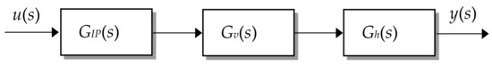
Figure 2.
An open-loop block diagram for regasification system.
3. The Proposed 2-DOF PID Controller
This section explains how to design a 2-DOF PID controller consisting of a set-point filter for reducing the overshoot in set-point tracking and a PID controller for eliminating the disturbance.
3.1. Structure of Control System
A closed-loop control system consisting of a set-point filter, a PID controller, and a regasification system model for an LNG-fueled marine engine is presented in Figure 3.
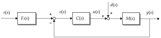
Figure 3.
The structure of control system with set-point filter.
Where , C(s), and M(s) are transfer functions of a set-point filter, a PID controller, and a regasification system, respectively. denotes the set-point input, the output temperature, and the disturbance. is the error between the set-point input and the measurement output, and is the control input.
3.2. Set-Point Filter
Since the proposed method focuses on eliminating disturbances, large overshoots may occur for changes in set-point inputs, and such large overshoots can be reduced using set-point filters. The output of a PID controller with a set-point filter is the same as the Equation (5).
where Kp, Ti, and Td represent the proportional gain, integral time, and derivative time of the PID controller, respectively. b has a value between 0 and 1 as a set-point weight factor. By transforming the Equation (5) into Laplace, the transfer function of the set-point filter as follows can be obtained.
3.3. Direct Synthesis Method
Direct synthesis (DS) is a method for designing a PID controller so that the closed-loop response of the control system matches the desired closed-loop response. Each parameter of the PID controller can be designed by matching the order and coefficients of the desired characteristic equation with those of the closed-loop characteristic equation of a control system consisting of a PID controller and a plant, etc.
Consider a first-order plus time delay model as shown in Equation (8).
where K, L, and T denote the gain, time delay, and time constant of the regasification system model, respectively.
The transfer function of the parallel PID controller to be designed is as follows.
The following characteristic equation is obtained from a closed-loop transfer function consisting of a model and a controller.
Using Pade’s first-order approximation , the above equation is written as follows
On simplifying and rearranging Equation (11), the following equation is obtained.
The desired closed-loop characteristic equation is given by
The above desired characteristic equation consists of three poles, which are located at . is a tuning parameter that is a time constant of the desired closed-loop transfer function, and on expanding Equation (13)
The following three equations are obtained by matching the coefficients of , , and in Equations (12) and (14).
By solving the Equations (15)–(17), the PID controller parameters are given as follows.
4. Parameter Tuning
To tune the PID controller parameters, the regasification system consisting of an I/P converter, diaphragm valve, and heat exchanger is first approximated to the FOPTD model. The parameter values for each element of the regasification system used in this paper are listed in Table 1.

Table 1.
Parameters of each element in the regasification system.
Figure 4 shows the screen of the system identification toolbox [32,33] for approximating the regasification system to an FOPTD model.
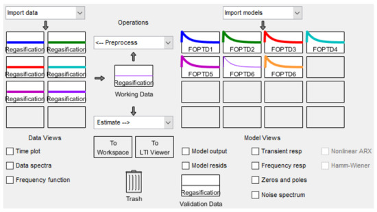
Figure 4.
Screen of the system identification toolbox for approximation with an FOPTD model.
The FOPTD model of the regasification system is obtained as K = 1.2508, L = 4.1, and T = 30.578 through several iterations in the identification toolbox of MATLAB using unit steps as input and glycol temperature as output. At this time, the sampling time is 0.01 s. The outputs and error when the unit step input is introduced to the original regasification open-loop system and the approximated FOPTD model are shown in Figure 5. The approximated model closely matches the original system.
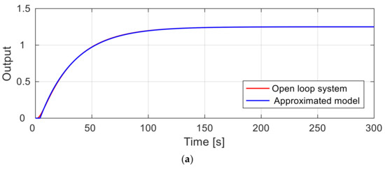
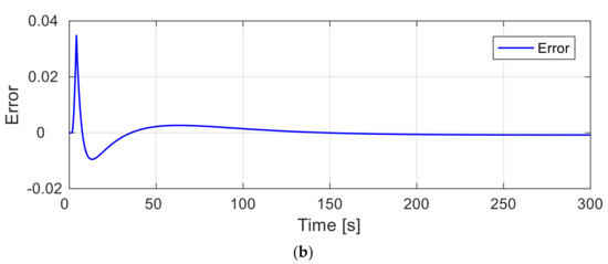
Figure 5.
Validation of the approximated FOPTD model. (a) Outputs; (b) Error.
The parameter values of the PID controller are obtained by substituting K, L, and T of the FOPTD model for the regasification system into Equations (18)–(20), which were derived in the previous Section. Table 2 summarizes the parameter values for PID controllers and weighting factor b for set-point filter. In addition, the controller parameters by the IMC method (hereafter, referred to as IMC) and by Skogestad’s method (hereafter, referred to as Skogestad) are listed together.
Table 2.
Parameter tuning for PID controllers.
5. Simulation
To show the effectiveness of the proposed controller, a series of simulations of glycol temperature control of LNG-fueled marine engines are performed.
The regasification system was approximated to an FOPTD model to design the PID controller, but the simulation is performed on the original regasification system. The response performance of the proposed method is compared with that of the IMC-based PID controller and PI controller by Skogestad [23]. For quantitative comparison in each simulation work, the performance measures such as rise time tr, 2% settling time ts, percentage overshoot (OS (%)), maximum peak error (Mpeak), 2% recovery time (trcy), and integral of absolute error (IAE) are calculated. Mpeak indicates |r − ymin| in disturbance response. The overall performance assessment is based on IAE, taking into account tr, ts, OS (%), trcy, and Mpeak. The smaller the IAE value, the better the overall performance. The simulation is performed in two cases. One is for a nominal heat exchanger where the parameter values of the heat exchanger have not changed, and the other is when the parameters of the heat exchanger are changed by 20% during operation to verify the robustness of the control system. It is assumed that the parameters changed by 20% due to uncertainty, but consider the worst case. Generally, in FOPTD models, it becomes difficult to control if the gain changes to the larger side and the time constant changes to the smaller side. Therefore, the gain of the heat exchanger is increased by 20% and the time constant is reduced by 20%.
5.1. Nominal Heat Exchanger
First, consider the nominal heat exchanger of the regasification system for LNG-fueled marine engines. A change in flow rate can be considered a disturbance because a change in the pressure of the steam can cause a change in the flow rate of steam through the valve, even if the opening of the valve is the same. The simulation results are shown in Figure 6 when step change from set-point 45 °C to 50 °C at t = 0 s and steam flow rate change of −0.5 kg/s at t = 100 s are applied as a disturbance in the nominal process. Performance measurements for quantitative comparison are tabulated in Table 3. As shown in Table 3 and Figure 6, all three methods in the set-point tracking response exhibit similar responses that converge to the desired value without steady-state error. On the other hand, the IMC method and the Skogestad’s method show a very long recovery time and a very large IAE in the disturbance rejection response. In particular, Skogestad’s method has a very large maximum peak error. However, the proposed method has a very short recovery time and a very small IAE compared to the other two methods. The proposed method reduced IAE by about 61–71% compared to the other two methods in the disturbance rejection response. The IAE value in the disturbance rejection response is smaller in the order of the proposed method, IMC method, and Skogestad’s method. Therefore, the proposed method performs best and Skogestad’s method is the worst.
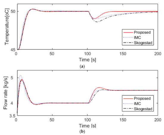
Figure 6.
Step responses and steam flow rate for nominal heat exchanger. (a) Step responses; (b) steam flow rate.
Table 3.
Comparison of performances for nominal heat exchanger.
5.2. Uncertain Heat Exchanger
The simulation process is subject to the same conditions as the nominal heat exchanger, except for changes in the parameters of the heat exchanger. The robustness is evaluated by simultaneously inserting 20% perturbations into each of the nominal parameters of heat exchanger towards the worst case parameter mismatch and assuming the actual process to be . Performance measurements for quantitative comparison are tabulated in Table 4. As shown in Figure 7 and Table 4, all three methods in the set-point tracking responses show similar responses that converge to the desired value without steady-state errors, but Skogestad’s method has a slightly longer settling time and larger percentage overshoot compared to the other two methods. On the other hand, the IMC method and the Skogestad’s method show a very long recovery time and a very large IAE in the disturbance rejection response. In particular, Skogestad’s method has a very large maximum peak error. However, the proposed method has a very short recovery time and a very small IAE compared to the other two methods. The proposed method reduced IAE by about 42–57% compared to the other two methods in the disturbance rejection response. The IAE value in the disturbance rejection response is smaller in the order of the proposed method, IMC method, and Skogestad’s method. Therefore, even if there is parameter uncertainty, the suggested method in the disturbance rejection response is the best and Skogestad’s method is the worst.
Table 4.
Comparison of performances for uncertain heat exchanger.
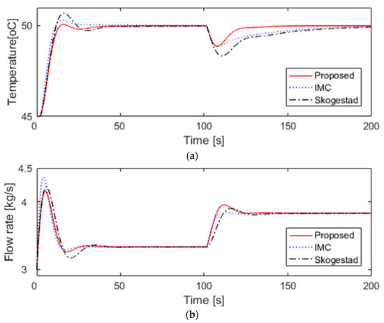
Figure 7.
Step responses and steam flow rate for uncertain heat exchanger. (a) Step responses; (b) steam flow rate.
5.3. Effect of Set-Point Filter
A set-point filter is used to reduce the overshoot in the set-point tracking response. The same controller that was previously designed is still used for the simulation. If a filter weighting value of b = 0.96 is used, the set-point filter, and if b = 1.0, the gain of the set-point filter will be 1, so the filter is not used. Figure 8 shows the closed-loop response by the proposed method for both with and without the set-point filter, and the performance indices such as tr, ts, OS(%), Mpeak, trcy, and IAE are listed in Table 5. When a set-point filter is used, the IAE value is reduced from 53.364 to 46.682, OS (%) from 2.926 to 0.602, and settling time from 35.475 to 30.694. As expected, using the set-point filter can improve the performance of the set-point tracking response, and Table 5 confirms that the set-point filter does not affect disturbance rejection performance at all.
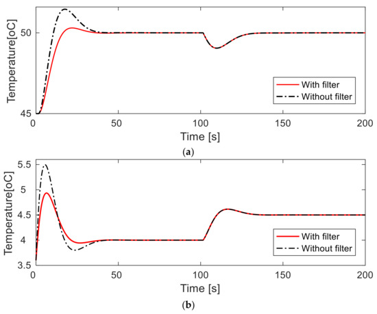
Figure 8.
Step responses and steam flow rate for nominal heat exchanger. (a) Step responses; (b) steam flow rate.
Table 5.
Effect of set-point filter for nominal heat exchanger.
6. Conclusions
In this paper, a DS-based 2-DOF PID controller was suggested to simultaneously improve the set-point tracking and input disturbance rejection performance for glycol temperature control of LNG-fueled marine engine, and how to tune the parameters of the PID controller was discussed. The 2-DOF PID controller comprises of a PID controller for rejecting an input disturbance in the regulatory response and a set-point filter for reducing the overshoot in the servo response.
The core contribution of this paper is that it is very easy to tune because there is only one adjustment variable for tuning the PID parameters, and the overshoot can be reduced by using a set-point filter. To show the effectiveness of the proposed method, a simulation of the glycol temperature control of the regasification system for LNG-fueled marine engines was performed and compared with the results of the two existing methods. In the case of nominal process, the proposed method reduced IAE by about 61–71% compared to the other methods, especially in the disturbance rejection response. In the case of parameter uncertainty, the proposed method decreased IAE by about 42–57% reduction in the disturbance rejection response. Using set-point filters reduces the IAE value from about 53 to 46, OS (%) from about 2.9 to 0.6, and settling time from about 35 to 30. The proposed controller was robust against uncertainty in heat exchanger parameters and was effective in both set-point tracking performance and disturbance rejection performance.
Funding
This research received no external funding.
Institutional Review Board Statement
Not applicable.
Informed Consent Statement
Not applicable.
Data Availability Statement
Not applicable.
Conflicts of Interest
The authors declare no conflict of interest.
References
- IMO Homepage. Available online: http://www.imo.org/en/OurWork/Environment/PollutionPrevention/Airpollution/Pages/Default.aspx (accessed on 22 March 2022).
- MAN Diesel & Turbo. ME-GI Duel Fuel MAN B&W Engines: A Technical, Operational and Cost-effective Solution for Ships Fuelled by Gas, MAN Diesel & Turbo 2012. Available online: https://www.man-es.com/?utm_medium=sea&utm_source=google&utm_campaign=always_sea_2022_man_brand_energy_solutions_bmm_all&utm_term=crossbrand&gclid=EAIaIQobChMI-P3bu6q29wIVYphmAh0kVwK7EAAYAiAAEgLbMfD_BwE&gclsrc=aw.ds (accessed on 22 March 2022).
- Jafarzadeh, S.; Paltrinieri, N.; Utne, I.B.; Ellingsen, H. LNG-fuelled fishing vessels: A systems engineering approach. Transp. Res. Part D Transp. Environ. 2017, 50, 202–222. [Google Scholar] [CrossRef]
- Åström, K.J.; Hägglund, T. Advanced PID Control; ISA: Pittsburgh, PA, USA, 2006. [Google Scholar]
- Choi, S. Configuration and analysis of a feed-forward control system for jacket cooling water temperature of marine prime diesel engine. J. Korean Soc. Mar. Eng. 2008, 32, 1303–1308. [Google Scholar]
- Ahn, J.K.; So, M.O. Cascade temperature control for jacket cooling water system of two-stroke low speed marine main diesel engine. J. Korean Soc. Mar. Eng. 2018, 42, 457–462. [Google Scholar]
- Vasičkaninová, A.; Bakošová, M. Control of heat exchanger using neural network predictive controller combined with auxiliary fuzzy controller. Appl. Therm. Eng. 2015, 89, 1046–1053. [Google Scholar] [CrossRef]
- Oravec, J.; Bakošová, M.; Mészáros, A.; Míková, N. Experimental investigation of alternative robust model predictive control of a heat exchanger. Appl. Therm. Eng. 2016, 105, 774–782. [Google Scholar] [CrossRef]
- Duka, A.V.; Oltean, S.E. Fuzzy control of a heat exchanger. In Proceedings of the 2012 IEEE International Conference on Automation Quality and Testing Robotics 2012, Cluj-Napoca, Romania, 24–27 May 2012; pp. 135–139. [Google Scholar]
- Beirami, H.; Zerafat, M.M. Self-tuning of an interval type-2 fuzzy PID controller for a heat exchanger system. Iran. J. Sci. Technol. Trans. Mech. Eng. 2015, 39, 113–129. [Google Scholar]
- Kumar, A.; Garg, K.K. Comparison of Ziegler-Nichols, Cohen-Coon and fuzzy logic controllers for heat exchanger model. Int. J. Sci. Eng. Technol. Res. 2015, 4, 1917–1920. [Google Scholar]
- Emhemed, A.A.A.; Alsseid, A.; Hanafi, D. Modelling and controller design for temperature control of power plant heat exchanger. Univers. J. Control Autom. 2017, 5, 49–53. [Google Scholar] [CrossRef]
- Padhee, S.; Khare, Y.B.; Singh, Y. Internal model based PID control of shell and tube heat exchanger system. In Proceedings of the IEEE Technology Students’ Symposium, Kharagpur, India, 14–16 January 2011; pp. 297–302. [Google Scholar]
- Padhee, S. Performance Evaluation of Different Conventional and Intelligent Controllers for Temperature Control of Shell and Tube Heat Exchanger System. Master’s Dissertation, Thapar University, Patiala Punjab, India, 2011. [Google Scholar]
- Padhee, S. Controller design for temperature control of heat exchanger system: Simulation studies. World Sci. Eng. Acad. Soc. (WSEAS) Trans. Syst. Control 2014, 9, 485–491. [Google Scholar]
- Khanvilkar, S.; Jadhav, S.P.; Vyawahare, V.; Kadam, V. Comparative study of fuzzy and IMC based controllers for heat exchanger system. In Proceedings of the 2016 International Conference on Automatic Control and Dynamic Optimization Techniques, Pune, India, 9–10 September 2016; pp. 344–348. [Google Scholar]
- Sarabeevi, G.M.; Beebi, M.L. Temperature control of shell and tube heat exchanger system using internal model controllers. In Proceedings of the 2016 International Conference on Next Generation Intelligent Systems, Kottayam, India, 1–3 September 2016. [Google Scholar]
- Manikandan, R.; Vinodha, R. Multiple model based adaptive control for shell and tube heat exchanger process. Int. J. Appl. Eng. 2016, 11, 3175–3180. [Google Scholar]
- Skorospeshkin, M.V.; Sukhodov, M.S.; Skorospeshkin, V.N.; Rymashevskiy, P.O. An adaptive control system for a shell-and-tube heat exchanger. In Proceedings of the International Conference on Information Technologies in Business and Industry, Journal of Physics: Conference Series, Tomsk, Russia, 21–26 September 2016. [Google Scholar]
- Xiao, Y.; Cui, G.; Chen, J.; Zhao, B. Improved model control strategy with dynamic adaption for heat exchangers in energy system. Int. J. Comput. Methodol. Numer. Heat Transf. Part A Appl. 2017, 72, 458–478. [Google Scholar] [CrossRef]
- Tavakoli, S.; Tavakoli, M. Optimal tuning of PID controller for first order plus time delay models using dimensional analysis. In Proceedings of the 4th International Conference on Control and Automation, Montreal, QC, Canada, 12 June 2003; pp. 942–946. [Google Scholar]
- Jin, G.G.; Son, Y.D. Design of a nonlinear controller and tuning rules for first-order plus time delay models. Stud. Inform. Control 2019, 28, 157–166. [Google Scholar] [CrossRef] [Green Version]
- Skogestad, S. Simple analytic rules for model reduction and PID controller tuning. J. Process Control 2003, 13, 291–309. [Google Scholar] [CrossRef] [Green Version]
- Lee, J.T.; Cho, W.H.; Edgar, T.F. Simple analytic PID controller tuning rules revisited. Ind. Eng. Chem. Res. 2014, 53, 5038–5047. [Google Scholar] [CrossRef]
- Shamsuzzoha, M. A unified approach for proportional-integral-derivative controller design for time delay processes. Korean J. Chem. Eng. 2015, 32, 583–596. [Google Scholar] [CrossRef]
- Chen, D.; Seborg, D.E. PI/PID controller design based on direct synthesis and disturbance rejection. Ind. Eng. Chem. Res. 2002, 41, 4807–4822. [Google Scholar] [CrossRef]
- Anil, C.; Sree, R.P. Tuning of PID controllers for integrating systems using direct synthesis method. ISA Trans. 2015, 57, 211–219. [Google Scholar] [CrossRef] [PubMed]
- So, H.R. Design of 2-DOF PID Controllers for First Order Plus Time Delay Systems Using Direct Synthesis Method. Ph.D. Thesis, Korea Maritime and Ocean University, Busan, Korea, 2022. [Google Scholar]
- Korkmaz, M.; Aydogdu, O.; Dogan, H. Design and performance comparison of variable parameter nonlinear PID controller and genetic algorithm based PID controller. In Proceedings of the 2012 Int. Symp. on Innovation in Intelligent Systems and Applications(INISTA), Trabzon, Turkey, 2–4 July 2012; pp. 1–5. [Google Scholar]
- So, G.B. Design of Nonlinear PID Controllers and Their Application to A Heat Exchanger System for LNG-Fuelled Marine Engines. Ph.D. Thesis, Korea Maritime and Ocean University, Busan, Korea, 2018. [Google Scholar]
- So, G.B. A modified 2-DOF control framework and GA based intelligent tuning of PID controllers. Processes 2021, 9, 1–19. [Google Scholar] [CrossRef]
- System Identification Toolbox, Getting Started Guide; Mathworks: Natick, MA, USA, 2020.
- System Identification Toolbox, User’s Guide; Mathworks: Natick, MA, USA, 2020.
Publisher’s Note: MDPI stays neutral with regard to jurisdictional claims in published maps and institutional affiliations. |
© 2022 by the author. Licensee MDPI, Basel, Switzerland. This article is an open access article distributed under the terms and conditions of the Creative Commons Attribution (CC BY) license (https://creativecommons.org/licenses/by/4.0/).