
Capabilities of an Acoustic Camera to Inform Fish Collision Risk with Current Energy Converter Turbines

 , and
, and
Abstract
:1. Introduction
2. Materials and Methods
2.1. Test Site 1
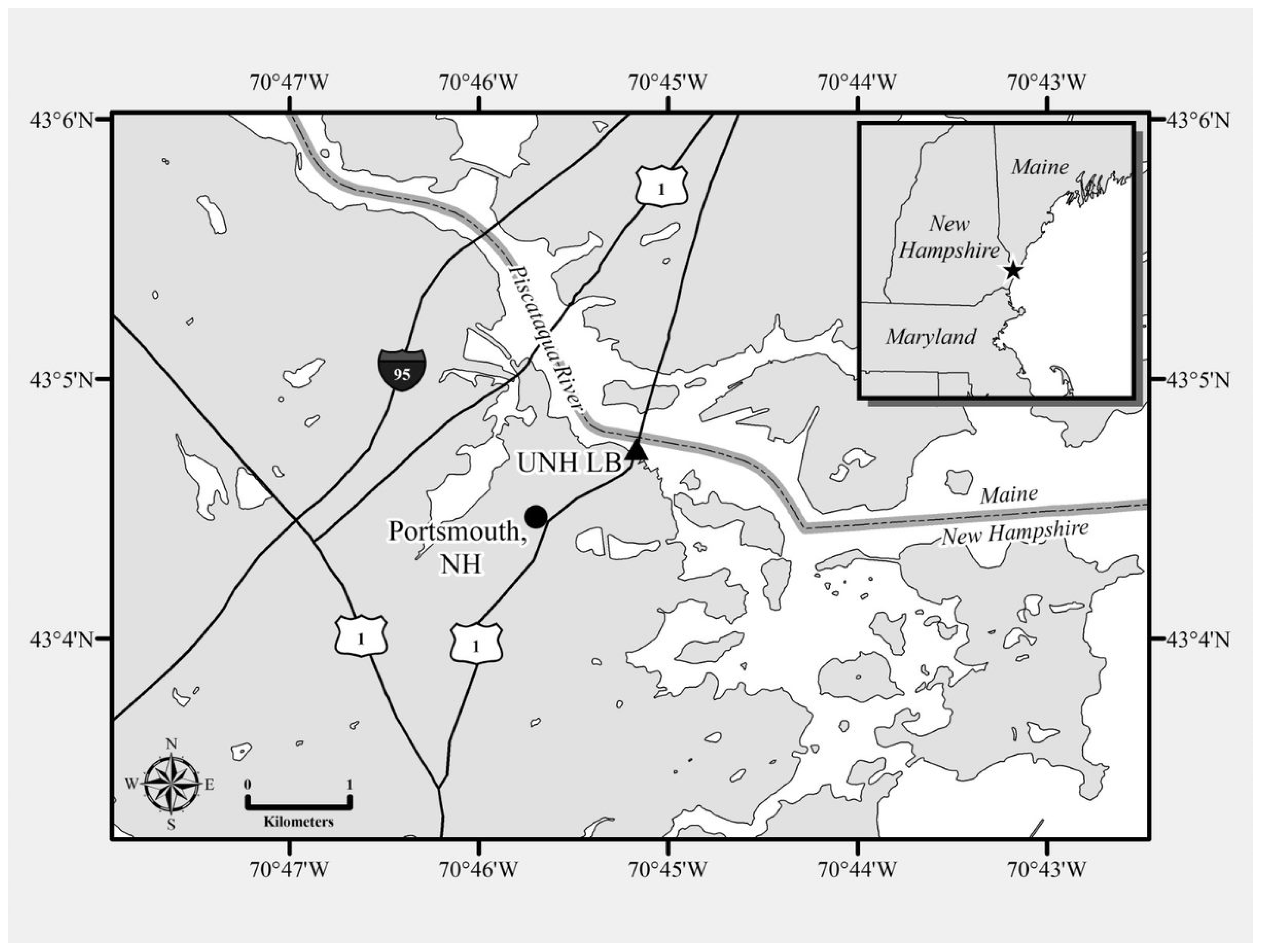
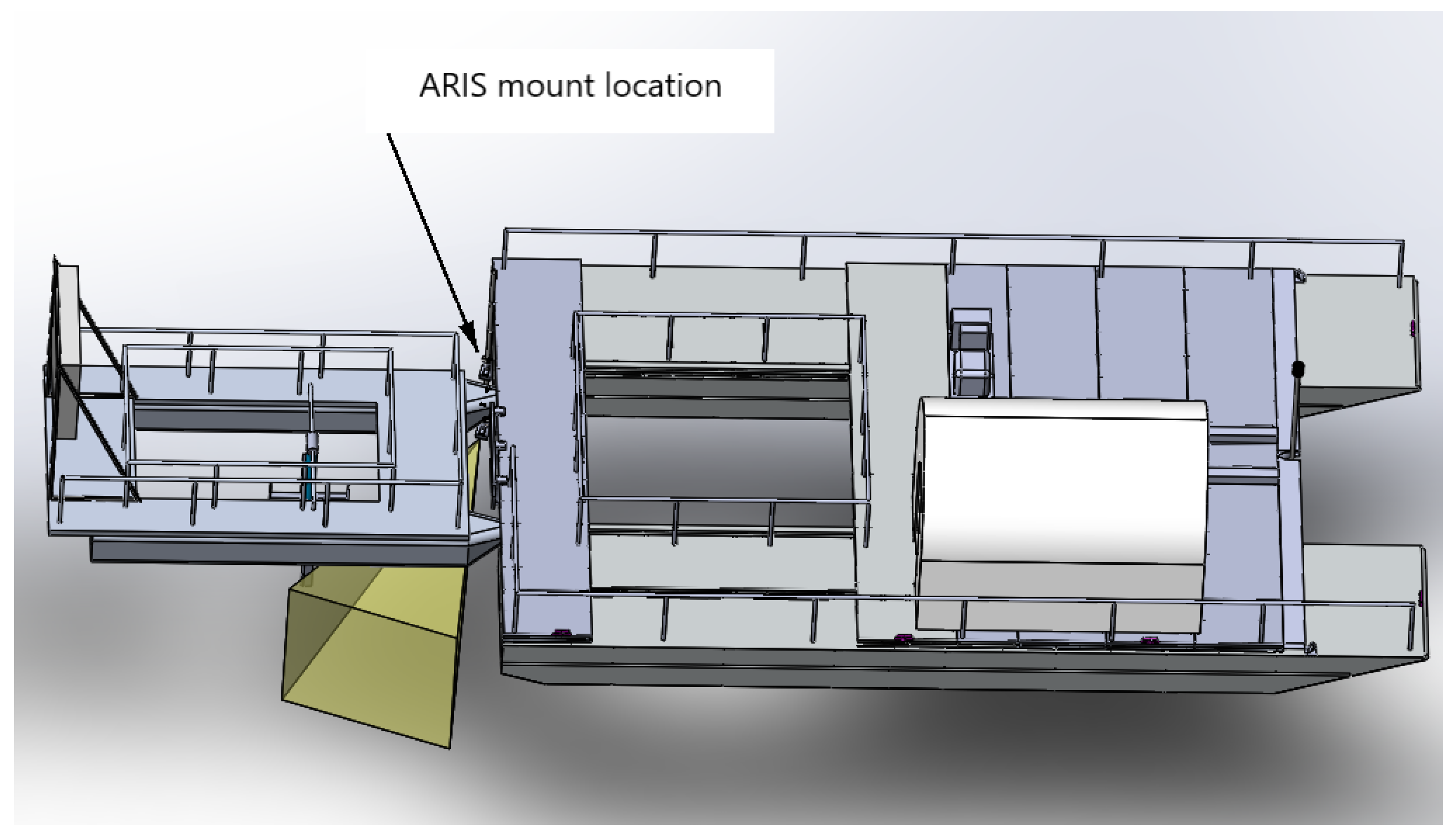
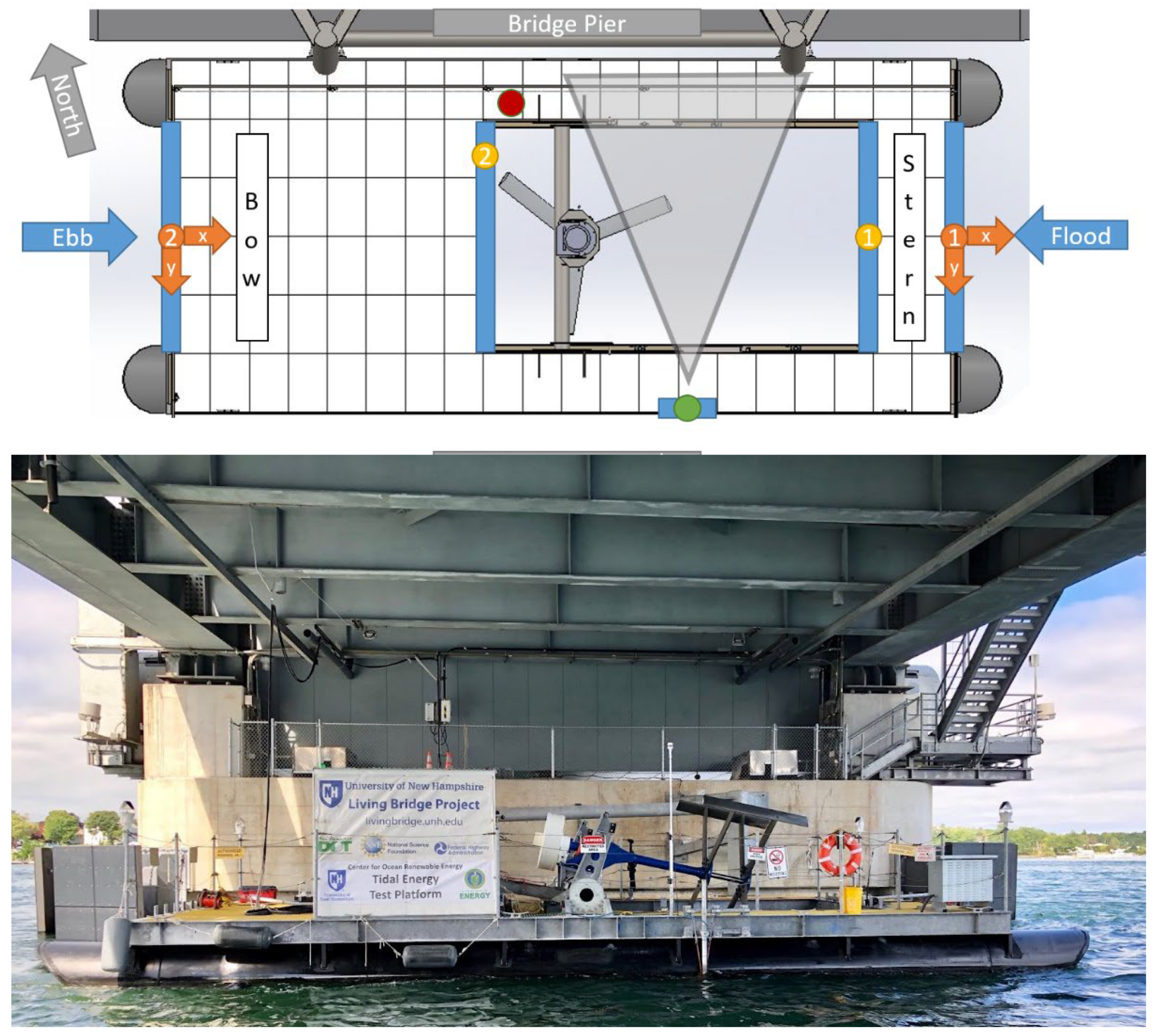
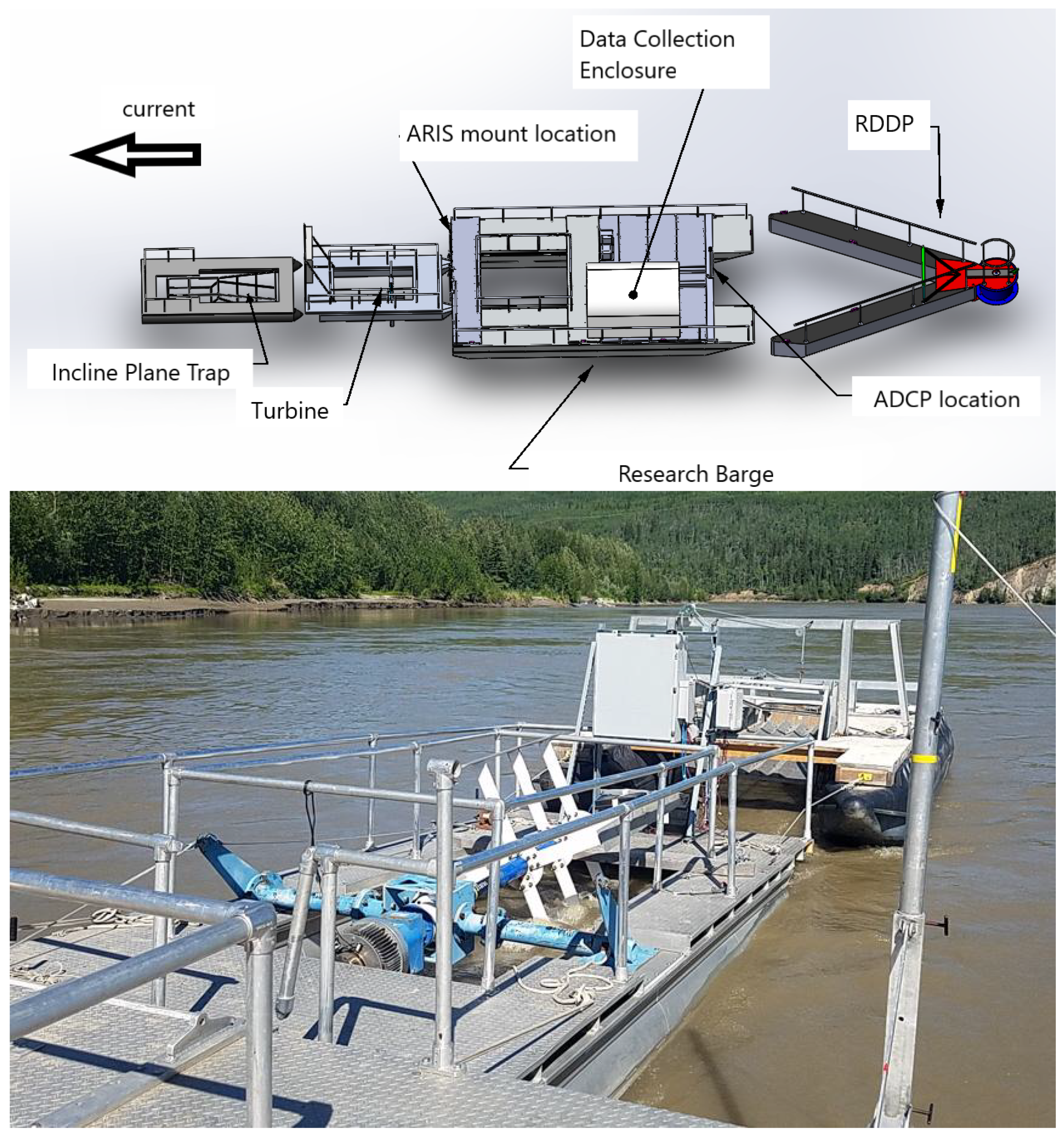
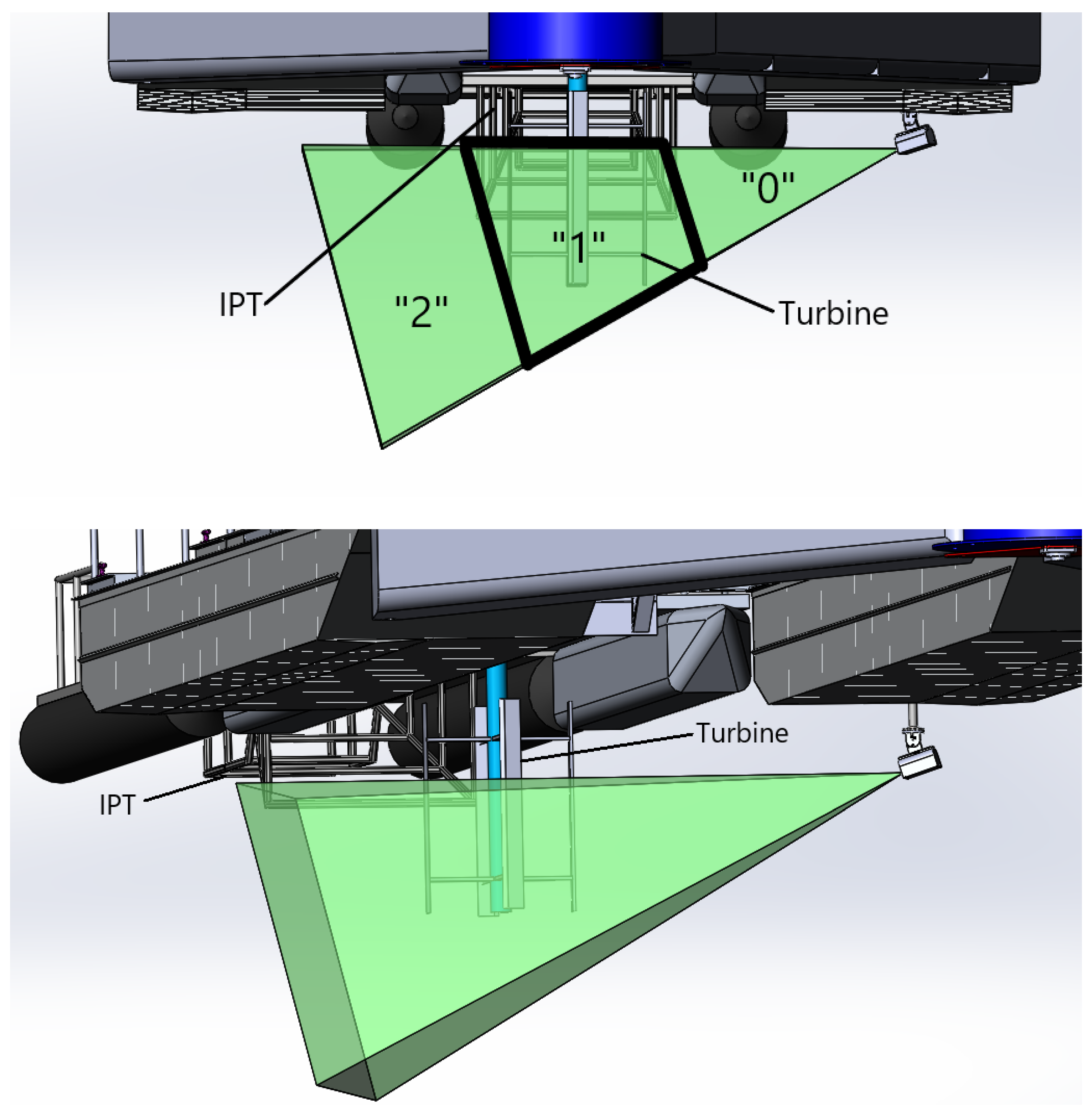
2.2. Test Site 2
2.2.1. Data Processing
2.2.2. Physical Fish Capture
3. Results
3.1. Test Site 1
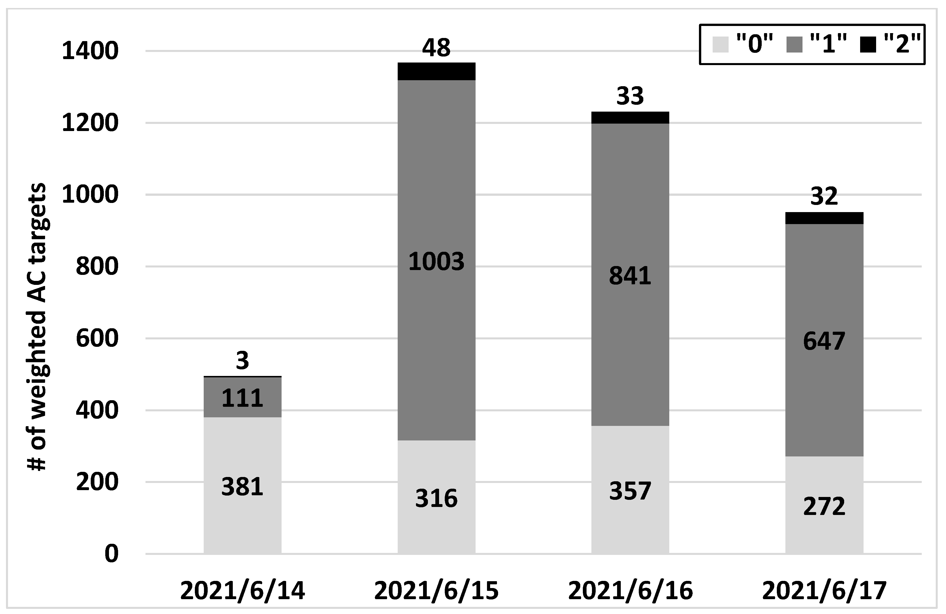
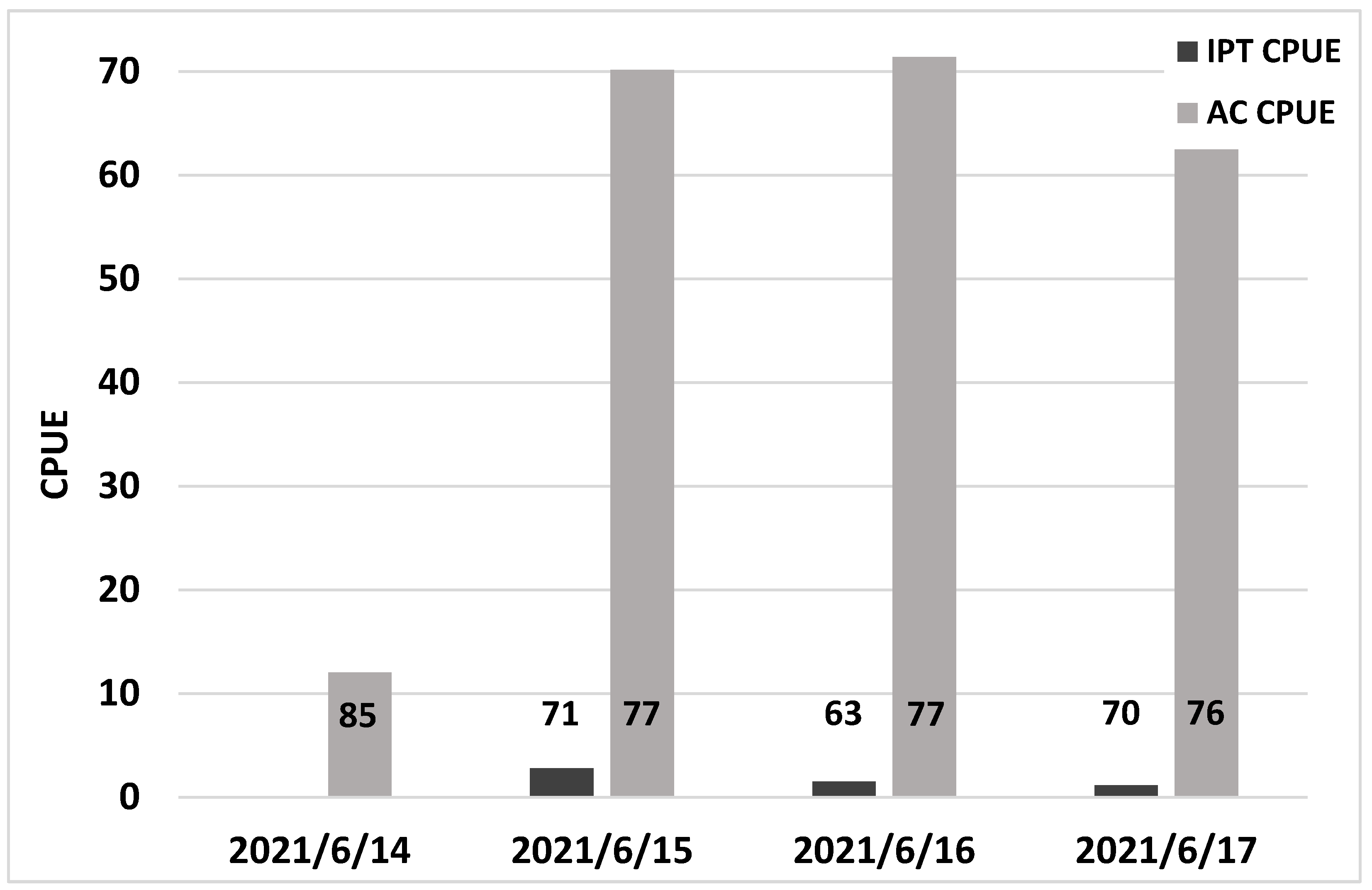
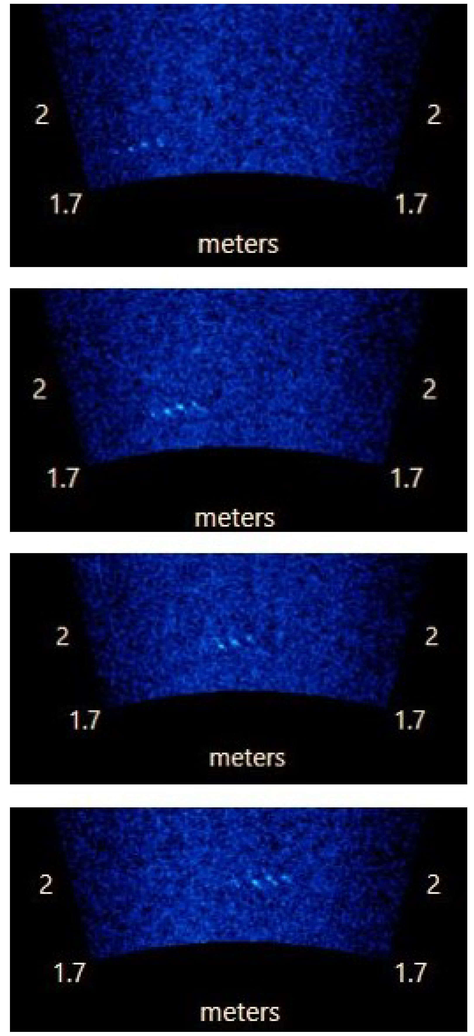
3.2. Test Site 2
4. Discussion
4.1. Test Site 1
4.2. Test Site 2
4.3. Recommendations and Future Research
4.3.1. Fish Strike Observation
4.3.2. Acoustic Camera Selection
4.3.3. Informing AC Targets with Catch Data
4.3.4. Modeling
5. Conclusions
Supplementary Materials
Author Contributions
Funding
Institutional Review Board Statement
Informed Consent Statement
Data Availability Statement
Acknowledgments
Conflicts of Interest
References
- Kilcher, L.; Fogarty, M.; Lawson, M. Marine Energy in the United States: An Overview of Opportunities; NREL/TP-5700-78773; National Renewable Energy Laboratory (NREL): Golden, CO, USA, 2021.
- Geerlofs, S. Marine energy and the new blue economy. In Preparing a Workforce for the New Blue Economy; Hotaling, L., Spinrad, R.W., Eds.; Elsevier: Cambridge, UK, 2021; pp. 171–178. [Google Scholar] [CrossRef]
- Kirke, B. Hydrokinetic turbines for moderate sized rivers. Energy Sustain. Dev. 2020, 58, 182–195. [Google Scholar] [CrossRef] [PubMed]
- Sparling, C.E.; Seitz, A.C.; Masden, E.; Smith, K. 2020 State of the Science Report, Chapter 3: Collision Risk for Animals around Turbines; Pacific Northwest National Laboratory: Richland, WA, USA, 2020; pp. 29–65.
- Hasselman, D.J.; Barclay, D.R.; Cavagnaro, R.; Chandler, C.; Cotter, E.; Gillespie, D.M.; Hastie, G.D.; Horne, J.K.; Joslin, J.; Long, C. 2020 State of the Science Report, Chapter 10: Environmental Monitoring Technologies and Techniques for Detecting Interactions of Marine Animals with Turbines; Pacific Northwest National Laboratory: Richland, WA, USA, 2020; pp. 176–213.
- Barr, Z.; Roberts, J.; Peplinski, W.; West, A.; Kramer, S.; Jones, C. The Permitting, Licensing and Environmental Compliance Process: Lessons and Experiences within US Marine Renewable Energy. Energies 2021, 14, 5048. [Google Scholar] [CrossRef]
- Peplinski, W.J.; Roberts, J.; Klise, G.; Kramer, S.; Barr, Z.; West, A.; Jones, C. Marine energy environmental permitting and compliance costs. Energies 2021, 14, 4719. [Google Scholar] [CrossRef]
- Hammar, L.; Andersson, S.; Eggertsen, L.; Haglund, J.; Gullström, M.; Ehnberg, J.; Molander, S. Hydrokinetic turbine effects on fish swimming behaviour. PLoS ONE 2013, 8, e84141. [Google Scholar] [CrossRef]
- Broadhurst, M.; Barr, S.; Orme, C.D.L. In-situ ecological interactions with a deployed tidal energy device; an observational pilot study. Ocean Coastal Man. 2014, 99, 31–38. [Google Scholar] [CrossRef]
- Matzner, S.; Trostle, C.K.; Staines, G.J.; Hull, R.E.; Avila, A.; Harker-Klimes, G.E. Triton: Igiugig Video Analysis-Project Report; PNNL-26576; Pacific Northwest National Laboratory: Richland, WA, USA, 2017.
- Nemeth, M.; Priest, J.; Patterson, H. Assessment of Fish and Wildlife Presence Near Two River Instream Energy Conversion Devices in The Kvichak River, Alaska in 2014; LGL Inc.: Sidney, BC, Canada, 2014. [Google Scholar]
- Viehman, H.A.; Zydlewski, G.B. Fish interactions with a commercial-scale tidal energy device in the natural environment. Estuaries Coasts 2015, 38, 241–252. [Google Scholar] [CrossRef]
- Bevelhimer, M.; Scherelis, C.; Colby, J.; Adonizio, M.A. Hydroacoustic assessment of behavioral responses by fish passing near an operating tidal turbine in the east river, New York. Trans. Am. Fish. Soc. 2017, 146, 1028–1042. [Google Scholar] [CrossRef]
- Williamson, B.J.; Blondel, P.; Williamson, L.D.; Scott, B.E. Application of a multibeam echosounder to document changes in animal movement and behaviour around a tidal turbine structure. ICES J. Mar. Sci. 2021, 78, 1253–1266. [Google Scholar] [CrossRef]
- Belcher, E.; Hanot, W.; Burch, J. Dual-frequency identification sonar (DIDSON). In Proceedings of the 2002 Interntional Symposium on Underwater Technology (Cat. No. 02EX556), Tokyo, Japan, 16–19 April 2002; pp. 187–192. [Google Scholar]
- Bilgili, A.; Proehl, J.A.; Lynch, D.R.; Smith, K.W.; Swift, M.R. Estuary/ocean exchange and tidal mixing in a Gulf of Maine Estuary: A Lagrangian modeling study. Estuar. Coast. Shelf Sci. 2005, 65, 607–624. [Google Scholar] [CrossRef]
- Kammerer, C. Tidal Currents in the Piscataqua River, NH: 2007 National Current Observation Program Survey; New Hampshire DES: Durham, NH, USA, 2007.
- Wosnik, M.; Chancey, K.; Gagnon, I.; Baldwin, K.; Bell, E. The ‘living bridge’ project: Tidal energy conversion at an estuarine bridge-Deployment and First Data. In Proceedings of the 6th Marine Energy Technology Symposium (METS), Washington, DC, USA, 30 April–2 May 2018. [Google Scholar]
- Chancey, K. Assessment of the Localized Flow and Tidal Energy Conversion System at an Estuarine Bridge; University of New Hampshire: Durham, NH, USA, 2019. [Google Scholar]
- Wosnik, M.; O’Byrne, P.; Chancey, K.; Gagnon, I.; Bell, E. A cost-effective grid-connected scaled tidal energy test site at Memorial Bridge in Portsmouth, New Hampshire, USA. In Proceedings of the International Conference on Ocean Energy, Virtual, 28–30 April 2021. [Google Scholar]
- Jump, S.; Courtney, M.B.; Seitz, A.C. Vertical distribution of juvenile salmon in a large turbid river. J. Fish. Wildl. Manag. 2019, 10, 575–581. [Google Scholar] [CrossRef] [Green Version]
- Johnson, J.; Toniolo, H.; Seitz, A.; Schmid, J.; Duvoy, P. Characterization of the Tanana River at Nenana, Alaska, to Determine the Important Factors Affecting Site Selection, Deployment, and Operation of Hydrokinetic Devices to Generate Power; Alaska Center for Energy and Power, Alaska Hydrokinetic Energy Research Center: Fairbanks, AK, USA, 2013; p. 130. [Google Scholar]
- Brabets, T.P.; Wang, B.; Meade, R.H. Environmental and Hydrologic Overview of the Yukon River Basin, Alaska and Canada; 99-4204; United States Geological Survey: Anchorage, AK, USA, 2000.
- Johnson, J.; Kasper, J.; Schmid, J.; Duvoy, P.; Kulchitsky, A.; Mueller-Stoffels, M.; Konefal, N.; Seitz, A. Surface Debris Characterization and Mitigation Strategies and Their Impact on the Operation of River Energy Conversion Devices on the Tanana River at Nenana, Alaska; Alaska Center for Energy and Power, Alaska Hydrokinetic Energy Research Center: Fairbanks, AK, USA, 2015. [Google Scholar]
- Seitz, A.C.; Moerlein, K.; Evans, M.D.; Rosenberger, A.E. Ecology of fishes in a high-latitude, turbid river with implications for the impacts of hydrokinetic devices. Rev. Fish Biol. Fish. 2011, 21, 481–496. [Google Scholar] [CrossRef]
- Bradley, P.T.; Evans, M.D.; Seitz, A.C. Characterizing the juvenile fish community in turbid Alaskan rivers to assess potential interactions with hydrokinetic devices. Trans. Am. Fish. Soc. 2015, 144, 1058–1069. [Google Scholar] [CrossRef]
- Todd, G.L. A lightweight, inclined-plane trap for sampling salmon smolts in rivers. Alaska Fish. Res. Bull. 1994, 1, 168–175. [Google Scholar]
- EPRI. Assessment of Technologies to Study Downstream Migrating American Eel Approach and Behavior at Iroquois Dam and Beauharnois Power Canal; 3002009406; Electric Power Research Institute: Palo Alto, CA, USA, 2017; p. 156. [Google Scholar]
- Viehman, H.A.; Zydlewski, G.B.; McCleave, J.D.; Staines, G.J. Using hydroacoustics to understand fish presence and vertical distribution in a tidally dynamic region targeted for energy extraction. Estuaries Coasts 2015, 38, 215–226. [Google Scholar] [CrossRef]
- Amaral, S.V.; Bevelhimer, M.S.; Čada, G.F.; Giza, D.J.; Jacobson, P.T.; McMahon, B.J.; Pracheil, B.M. Evaluation of behavior and survival of fish exposed to an axial-flow hydrokinetic turbine. N. Am. J. Fish. Manag. 2015, 35, 97–113. [Google Scholar] [CrossRef]
- Castro-Santos, T.; Haro, A. Survival and behavioral effects of exposure to a hydrokinetic turbine on juvenile Atlantic salmon and adult American shad. Estuaries Coasts 2015, 38, 203–214. [Google Scholar] [CrossRef]
- Cook, D.; Middlemiss, K.; Jaksons, P.; Davison, W.; Jerrett, A. Validation of fish length estimations from a high frequency multi-beam sonar (ARIS) and its utilisation as a field-based measurement technique. Fish. Res. 2019, 218, 59–68. [Google Scholar] [CrossRef]
- Kimball, M.E.; Rozas, L.P.; Boswell, K.M.; Cowan, J.H., Jr. Evaluating the effect of slot size and environmental variables on the passage of estuarine nekton through a water control structure. J. Exp. Mar. Biol. Ecol. 2010, 395, 181–190. [Google Scholar] [CrossRef]
- Able, K.W.; Grothues, T.M.; Rackovan, J.L.; Buderman, F.E. Application of Mobile Dual-frequency Identification Sonar (DIDSON) to Fish in Estuarine Habitats. Northeast. Nat. 2014, 21, 192–209. [Google Scholar] [CrossRef]
- Burwen, D.L.; Fleischman, S.J.; Miller, J.D. Accuracy and precision of salmon length estimates taken from DIDSON sonar images. Trans. Am. Fish. Soc. 2010, 139, 1306–1314. [Google Scholar] [CrossRef]
- Mueller, A.-M.; Burwen, D.L.; Boswell, K.M.; Mulligan, T. Tail-beat patterns in dual-frequency identification sonar echograms and their potential use for species identification and bioenergetics studies. Trans. Am. Fish. Soc. 2010, 139, 900–910. [Google Scholar] [CrossRef]
- Helminen, J.; O’Sullivan, A.M.; Linnansaari, T. Measuring Tailbeat Frequencies of Three Fish Species from Adaptive Resolution Imaging Sonar Data. Trans. Am. Fish. Soc. 2021, 150, 627–636. [Google Scholar] [CrossRef]
- Martignac, F.; Daroux, A.; Bagliniere, J.L.; Ombredane, D.; Guillard, J. The use of acoustic cameras in shallow waters: New hydroacoustic tools for monitoring migratory fish population. A review of DIDSON technology. Fish Fish. 2015, 16, 486–510. [Google Scholar] [CrossRef]
- Arnold, G. Movements of fish in relation to water. In Animal Migration; Aidley, D.J., Ed.; Cambridge University Press: New York, NY, USA, 1981; Volume 13, p. 55. [Google Scholar]
- Simmonds, E.J. Fisheries Acoustics: Theory and Practice; John Wiley & Sons: Hoboken, NJ, USA, 2008. [Google Scholar]
- Holmes, J.A.; Cronkite, G.M.; Enzenhofer, H.J.; Mulligan, T.J. Accuracy and precision of fish-count data from a “dual-frequency identification sonar” (DIDSON) imaging system. ICES J. Mar. Sci. 2006, 63, 543–555. [Google Scholar] [CrossRef] [Green Version]
- Mueller, A.-M.; Mulligan, T.; Withler, P.K. Classifying sonar images: Can a computer-driven process identify eels? N. Am. J. Fish. Manag. 2008, 28, 1876–1886. [Google Scholar] [CrossRef] [Green Version]
- Balk, H.; Lindem, T.; Kubecka, J. New Cubic Cross filter detector for multi beam data recorded with DIDSON acoustic camera. In Proceedings of the 3rd International Conference & Exhibition Underwater Acoustic Measurements: Technologies & Results, Peloponnese, Greece, 21–26 June 2009. [Google Scholar]
- Petreman, I.C.; Jones, N.E.; Milne, S.W. Observer bias and subsampling efficiencies for estimating the number of migrating fish in rivers using Dual-frequency IDentification SONar (DIDSON). Fish. Res. 2014, 155, 160–167. [Google Scholar] [CrossRef]
- Pham, A.H.; Lundgren, B.; Stage, B.; Jensen, J.A. Ultrasound backscatter from free-swimming fish at 1 MHz for fish identification. In Proceedings of the 2012 IEEE International Ultrasonics Symposium, Dresden, Germany, 7–10 October 2012; pp. 1477–1480. [Google Scholar]
- Staines, G.; Zydlewski, G.B.; Viehman, H.A.; Kocik, R. Applying Two Active Acoustic Technologies to Document Presence of Large Marine Animal Targets at a Marine Renewable Energy Site. J. Mar. Sci. Eng. 2020, 8, 704. [Google Scholar] [CrossRef]
- Medwin, H.; Clay, C.S. Fundamentals of Acoustical Oceanography; Academic Press: Cambridge, MA, USA, 1998. [Google Scholar] [CrossRef]
- Maxwell, S.L.; Gove, N.E. Assessing a dual-frequency identification sonars’ fish-counting accuracy, precision, and turbid river range capability. J. Acoust. Soc. Am. 2007, 122, 3364–3377. [Google Scholar] [CrossRef]
- Richards, S.; Leighton, T. High frequency sonar performance predictions for littoral operations—the effects of suspended sediments and microbubbles. J. Def. Sci. 2003, 8, 1–7. [Google Scholar]
- Richards, S.; White, P.; Leighton, T. Volume absorption and volume reverberation due to microbubbles and suspended particles in a ray-based sonar performance model. In Proceedings of the Seventh European Conference on Underwater Acoustics, Delft, The Netherlands, 5–8 July 2004; pp. 173–178. [Google Scholar]
- Dahl, P.H.; Geiger, H.J.; Hart, D.A.; Dawson, J.J.; Johnston, S.V. The Environmental Acoustics of Two Alaskan Rivers and Its Relation to Salmon Counting Sonars; University of Washington: Seattle, WA, USA, 2001; p. 40. [Google Scholar]
- Young, D.L.; McFall, B.C.; Bryant, D.B. Bubble image velocimetry with a field-deployable acoustic camera. Meas. Sci. Technol. 2018, 29, 125302. [Google Scholar] [CrossRef]
- Martinez, J.J.; Deng, Z.; Titzler, P.S.; Duncan, J.P.; Lu, J.; Mueller, R.P.; Tian, C.; Trumbo, B.A.; Ahmann, M.L.; Renholds, J.F. Hydraulic and biological characterization of a large Kaplan turbine. Renew. Energy 2019, 131, 240–249. [Google Scholar] [CrossRef]
- Deng, Z.; Duncan, J.; Arnold, J.; Fu, T.; Martinez, J.; Lu, J.; Titzler, P.; Zhou, D.; Mueller, R. Evaluation of boundary dam spillway using an autonomous sensor fish device. J. Hydro-Environ. Res. 2017, 14, 85–92. [Google Scholar] [CrossRef] [Green Version]
- Zang, X.; Yin, T.; Hou, Z.; Mueller, R.P.; Deng, Z.D.; Jacobson, P.T. Deep learning for automated detection and identification of migrating American eel Anguilla rostrata from imaging sonar data. Remote Sens. 2021, 13, 2671. [Google Scholar] [CrossRef]
- Cotter, E.; Polagye, B. Detection and classification capabilities of two multibeam sonars. Limnol. Oceanogr. Methods 2020, 18, 673–680. [Google Scholar] [CrossRef]
- Francisco, F.; Sundberg, J. Detection of visual signatures of marine mammals and fish within marine renewable energy farms using multibeam imaging sonar. J. Mar. Sci. Eng. 2019, 7, 22. [Google Scholar] [CrossRef] [Green Version]
- Buenau, K.E.; Garavelli, L.; Hemery, L.G.; García Medina, G. A Review of Modeling Approaches for Understanding and Monitoring the Environmental Effects of Marine Renewable Energy. J. Mar. Sci. Eng. 2022, 10, 94. [Google Scholar] [CrossRef]


| Target | Length (cm) | Material | Current Velocity (m·s−1) | Turbine 1 RPMs | Supplementary Video |
|---|---|---|---|---|---|
| 1 | 8.0 | Hard plastic | 0.85 | 13.4 | Video S1 |
| 2 | 10.0 | Hard plastic | 0.90 | 11.9 | Video S2 |
| 3 | 10.0 | Hard plastic | 0.71 | 14.0 | Video S3 |
| 4 | 10.5 | Soft rubber | 0.80 | 11.8 | Video S4 |
| Day | Tilt (deg) | Depth (m) | Turbidity NTUs 1 | Mean Current Velocity (m·s−1) | Average Discharge (m3·s−1) | Data Volume (h, GB) |
|---|---|---|---|---|---|---|
| 14 June | 0.0 | 0.75 | 211 | n/d | 1113 | 3.1, 22 |
| 15 June | −0.4 | 2.4 | 209 | 1.67 | 1138 | 4.8, 34 |
| 16 June | −9.7 | 1.0 | 227 | 1.64 | 1175 | 3.9, 28 |
| 17 June | −9.4 | 1.0 | 263 | 1.71 | 1223 | 3.5, 25 |
| Event | Date | Time | Species | Fork Length (mm) | IPT Recapture (Y/N) | Re-Release After Recapture? (Y/N) | Visually Detected (Y/N/M) 1 |
|---|---|---|---|---|---|---|---|
| 1 | 14 June 2021 | 15:51:00 | LNS | 70 | N | NA | N |
| CHB | 120 | N | NA | ||||
| LNS | 60 | N | NA | ||||
| 2 | 15 June 2021 | 13:48:27 | LNS | 48 | N | NA | Y |
| 3 | 16 June 2021 | 12:27:18 | LNS | 40 | N | NA | Y; M |
| LNS | 45 | Y | NA | ||||
| LNS | 45 | Y | NA | ||||
| LNS | 45 | N | NA | ||||
| CHB | 65 | N | NA | ||||
| CHB | 50 | N | NA | ||||
| 4 | 16 June 2021 | 12:40:19 | LNS | 45 | N | Y | N |
| LNS | 45 | N | Y | ||||
| 5 | 17 June 2021 | 11:26:28 | LNS | 65 | Y | NA | N |
| LNS | 80 | N | NA | ||||
| LNS | 55 | N | NA | ||||
| CHB | 100 | N | NA | ||||
| 6 | 17 June 2021 | 11:30:22 | LNS | 65 | N | Y | N |
| 7 | 17 June 2021 | 16:35:20 | CHB | 70 | N | NA | M |
| CHB | 70 | N | NA |
Publisher’s Note: MDPI stays neutral with regard to jurisdictional claims in published maps and institutional affiliations. |
© 2022 by the authors. Licensee MDPI, Basel, Switzerland. This article is an open access article distributed under the terms and conditions of the Creative Commons Attribution (CC BY) license (https://creativecommons.org/licenses/by/4.0/).
Share and Cite
Staines, G.J.; Mueller, R.P.; Seitz, A.C.; Evans, M.D.; O’Byrne, P.W.; Wosnik, M. Capabilities of an Acoustic Camera to Inform Fish Collision Risk with Current Energy Converter Turbines. J. Mar. Sci. Eng. 2022, 10, 483. https://doi.org/10.3390/jmse10040483
Staines GJ, Mueller RP, Seitz AC, Evans MD, O’Byrne PW, Wosnik M. Capabilities of an Acoustic Camera to Inform Fish Collision Risk with Current Energy Converter Turbines. Journal of Marine Science and Engineering. 2022; 10(4):483. https://doi.org/10.3390/jmse10040483
Chicago/Turabian StyleStaines, Garrett J., Robert P. Mueller, Andrew C. Seitz, Mark D. Evans, Patrick W. O’Byrne, and Martin Wosnik. 2022. "Capabilities of an Acoustic Camera to Inform Fish Collision Risk with Current Energy Converter Turbines" Journal of Marine Science and Engineering 10, no. 4: 483. https://doi.org/10.3390/jmse10040483