
Emphasis on Occupancy Rates in Carbon Emission Comparison for Maritime and Road Passenger Transportation Modes


Abstract
:1. Introduction
- The 2011 White Paper from the European Commission, “Roadmap to a Single European Transport Area” [16], where the general premises are set. Among these are mentioned: the reduction of 40% of maritime transport emissions by 2050 compared to 2005, the simplification of procedures for travelers within the “European Blue Belt”, and the enhancement of safety, security, and environmental protection through the SafeSeaNet of the EMSA (European Maritime Safety Agency).
- Communication 2009-8 of the EC [17], which highlights, among the rest: the need to improve environmental performance through incentives and taxation measures, to support actions specifically aimed at greener shipping, technological innovation, the enhancement of short-sea transport services, and the promotion of a European Environmental Management System for Maritime Transport (EMS-MT).
- The “European Green Deal” and its annex [18], which defines the agenda and the roadmap for a set of “deeply transformative policies”, specifying a long list of prerequisites and targets that development must abide by in order to be effectively “sustainable”, in the sense of increasing the social, environmental, and economic capital of the EU member states. Particularly, the EC strategy for the improvement of the environmental performance of maritime transport (COM2009-8 final) specifically mentions a comprehensive approach to reducing greenhouse gas emissions from international shipping, combining technical, operational, and market-based measures.
2. Materials and Methods
2.1. Framework for Calculating Carbon Emissions
- If the passenger line is operated by the HSC, “Cold ironing” means that all technical systems on board are turned off.
- If the passenger line is operated by the RO-PAX ferry vessel, “Cold ironing” means that the all engines are turned off, and electrical power must be supplied from shore to vessel with a zero-emission source.
- Auxiliary engine power for RO-PAX ferry vessels—10% of main propulsion engine(s) power.
- Auxiliary engine power for HSC—5% of main propulsion engine(s) power.
- During navigation (), auxiliary engines are considered to be in operation, and carbon emission is calculated according to (3).
- Port stay ship operation () consists of the hoteling phase, where auxiliary engines are operated, and carbon emission is calculated according to (4).
- During the maneuvering phase, the propulsion engine load is estimated as during navigation, and the auxiliary engine load is estimated based on the earlier-mentioned methodology.
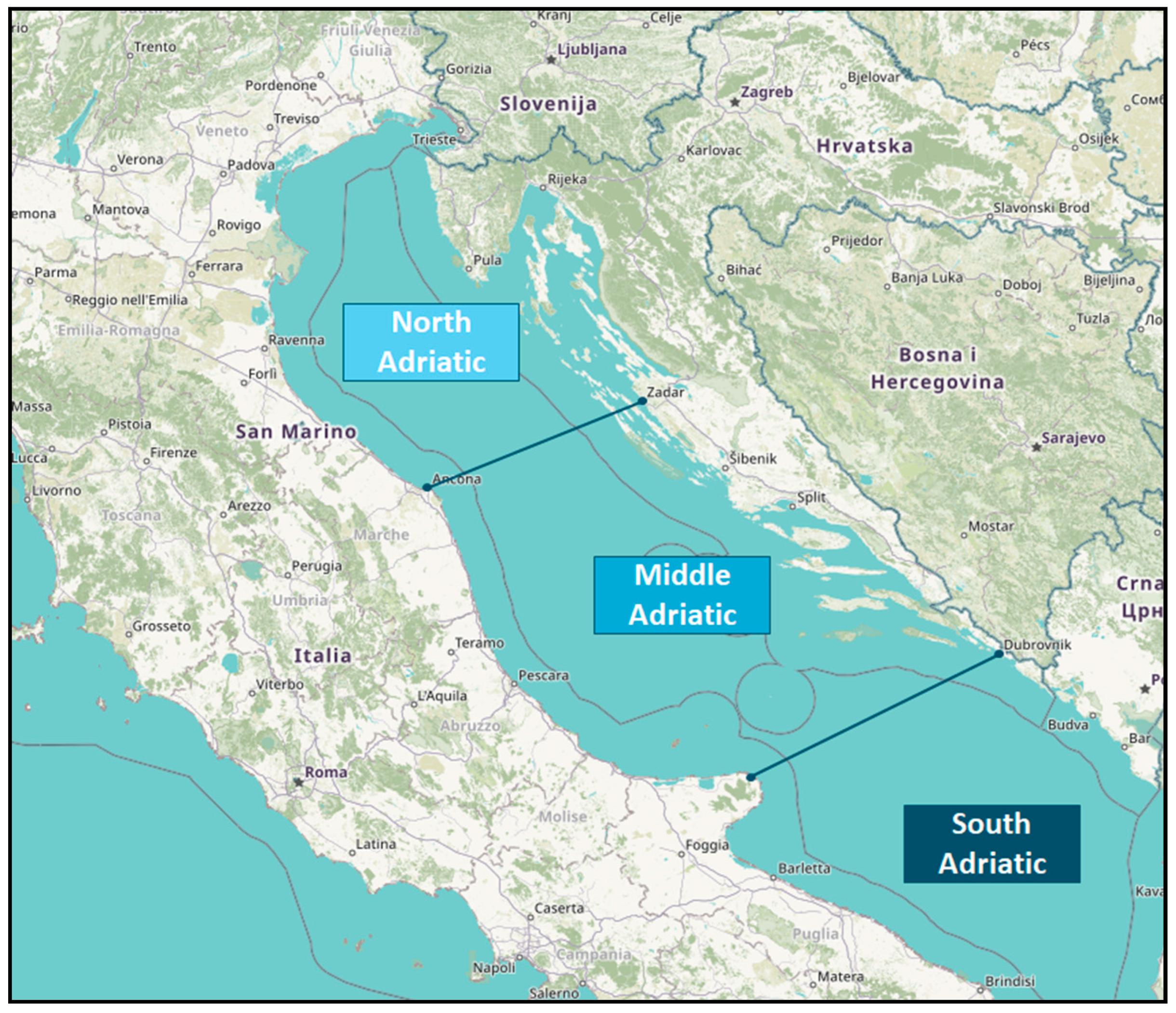
2.2. Italy–Croatia Interconnection Network and Chosen Routes
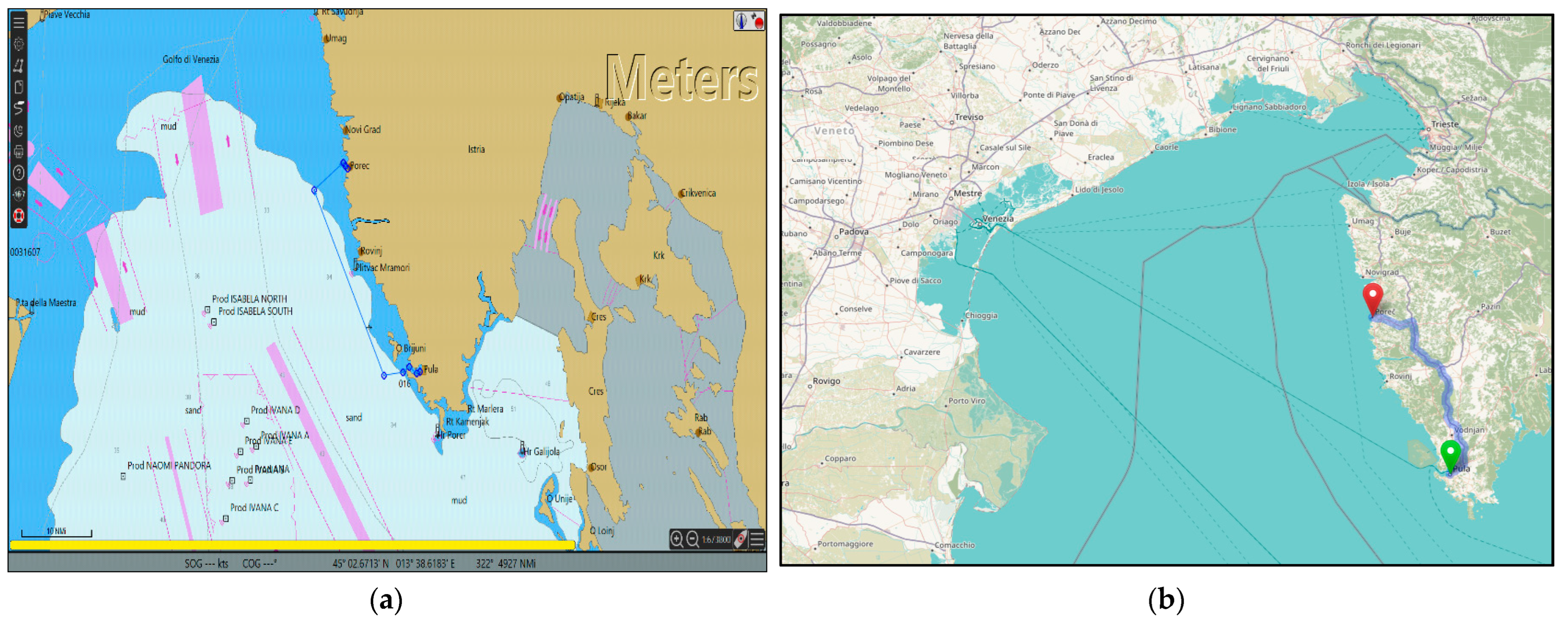
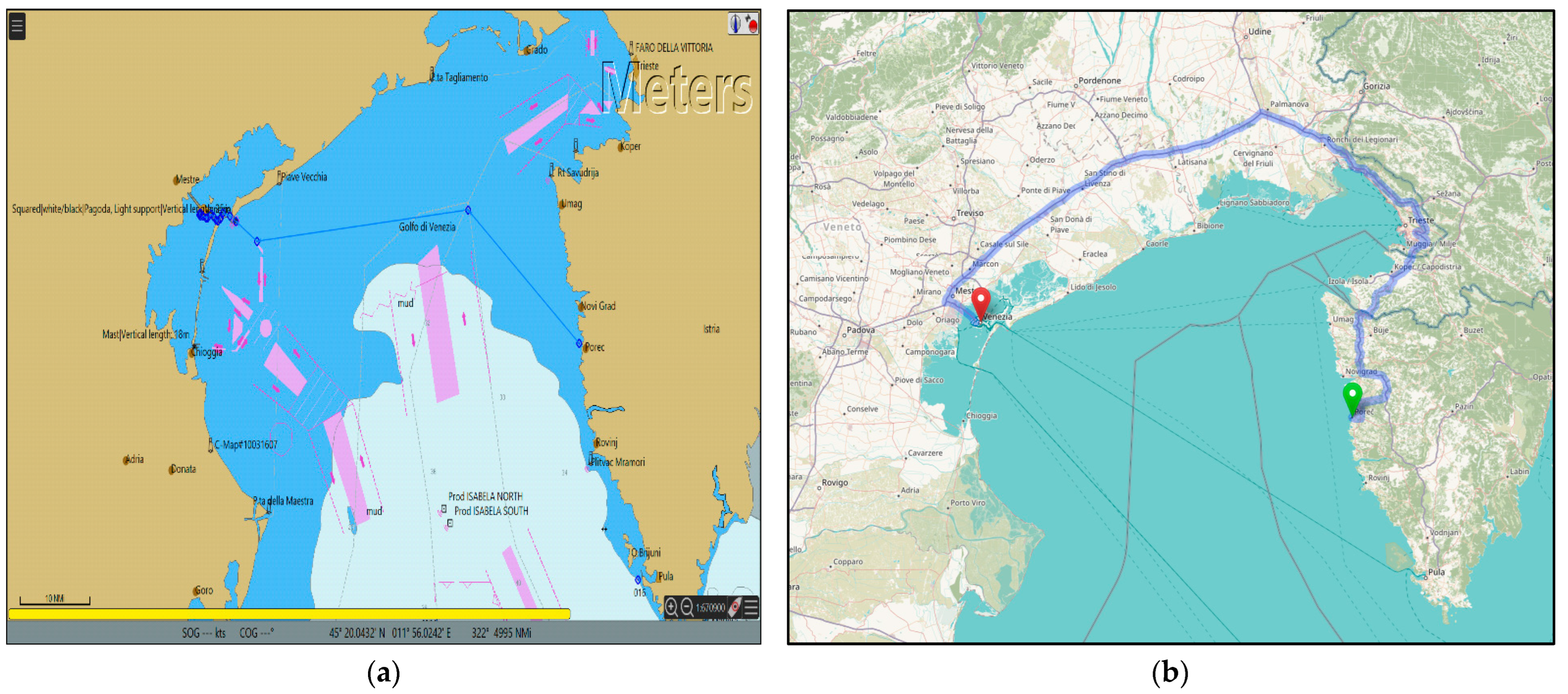
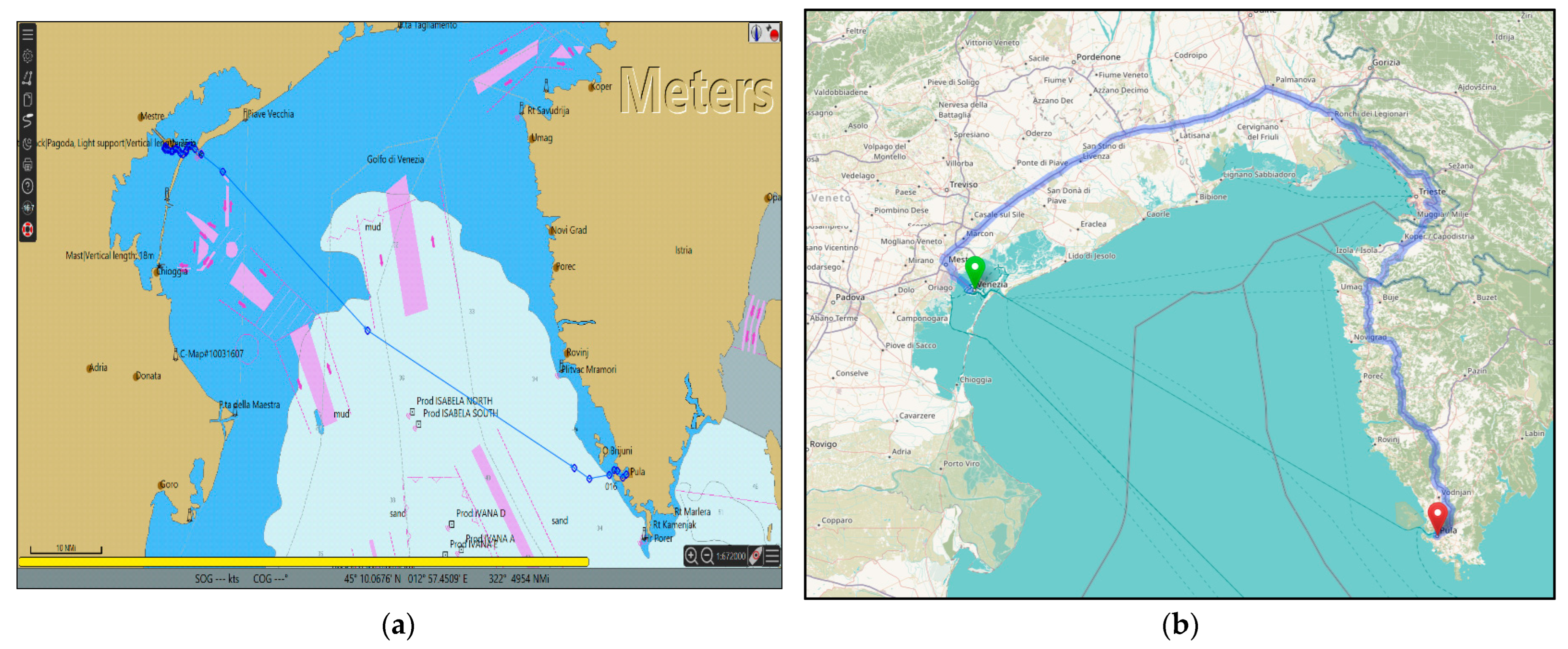
- Case study 1: Venice–Pula–Poreč–Venice ().
- Case study 2: Zadar–Ancona ().
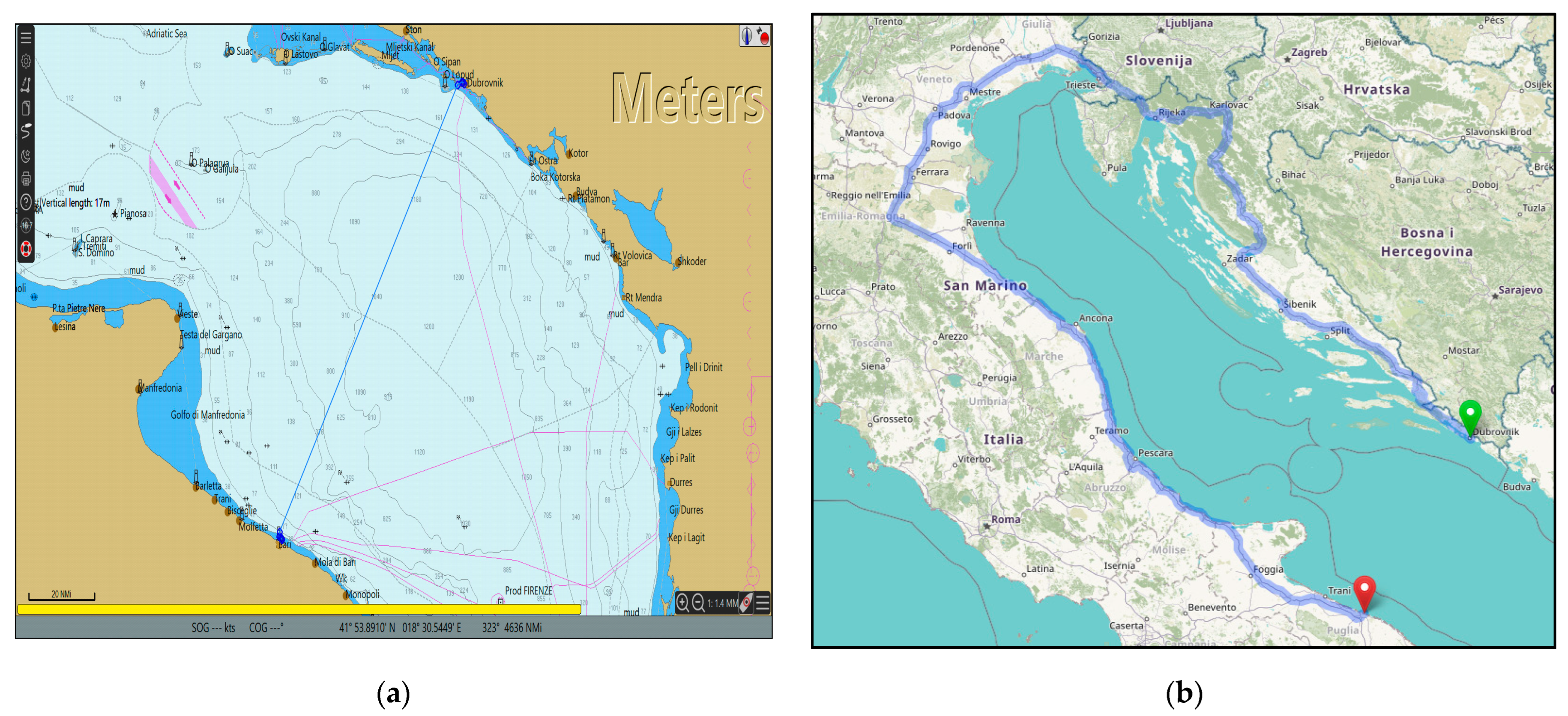
- Case study 3: Bari–Dubrovnik ().
3. Routes Analysis and Calculation Results
3.1. Venice–Pula–Poreč (R1)
- 3.31 passenger/car for route segment.
- 3.26 passenger/car for route segment.

- Italy: highway SR11 and motorway A4 (part of European route E70) from Venice to Trieste.
- Slovenia: highways H5 and H6 (part of European route E751) from border crossing Škofija to border crossing Dragonja.
- Croatia: motorway A9 (part of European route E751) from Dragonja to Pula.
- Croatia: motorway A9 (part of European route E751) and
- State road D302 from Pula to Baderna and from Baderna to Poreč, respectively.
- Croatia: state road D302 and motorway A9 (part of European route E751) from Poreč to Baderna and from Baderna to Dragonja, respectively.
- Slovenia: highway H5 and H6 (part of European route E751) from border crossing Dragonja to border crossing Škofija.
- Italy: motorway A4 and highway SR11 (part of European route E70) from Trieste to Venice.
3.2. Zadar–Ancona ()
- 3.25 passenger/car for entry into Croatia—route Ancona–Zadar,
- 3.28 passenger/car for exiting from Croatia—route Zadar–Ancona.
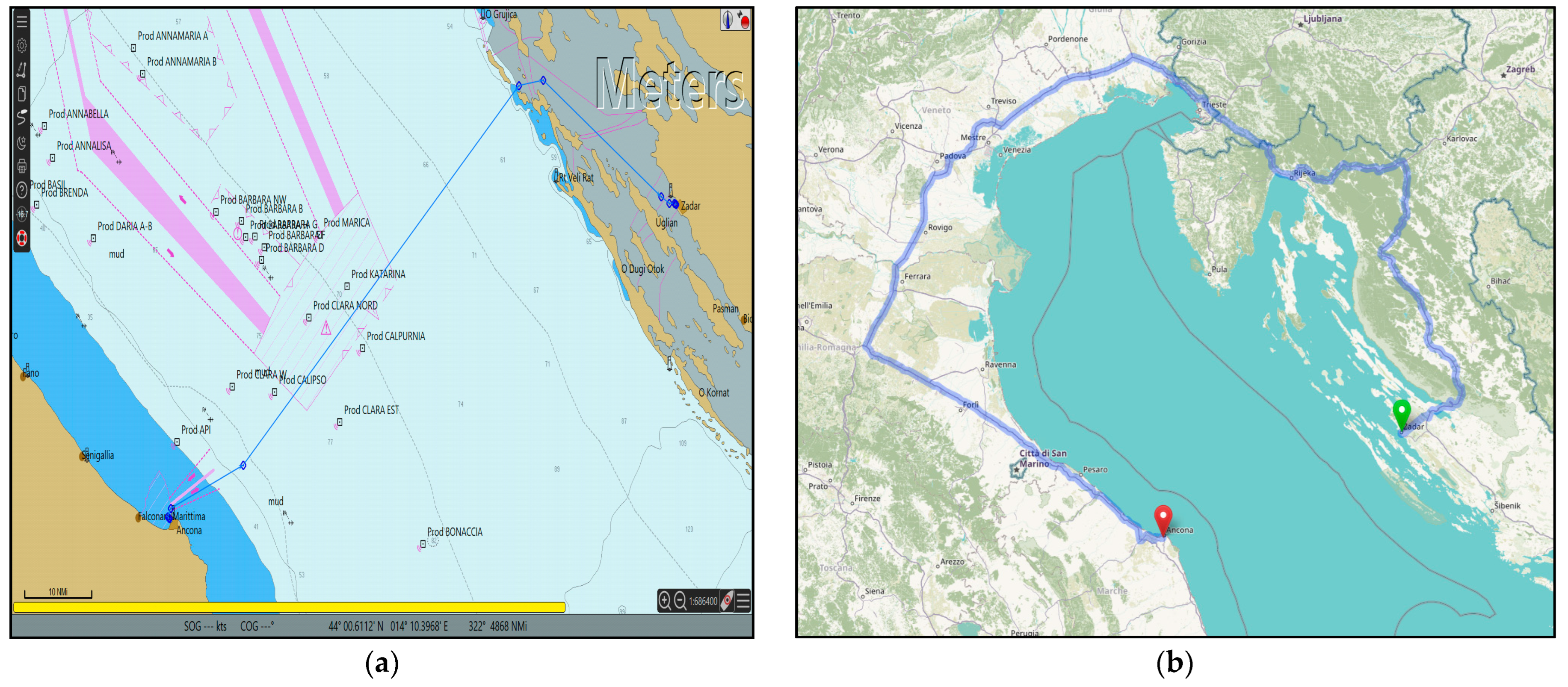
- Italy: motorway A14 (part of European route E55), A13, A4, and highway SS14 from Ancona to Bologna, from Bologna to Padua, from Padua to Trieste, and from Trieste to border crossing Krvavi Potok, respectively.
- Slovenia: state road G7 from border crossing Krvavi Potok to Starod.
- Croatia: highway D8, motorways A7, A6, A1, and state road D424 from Pasjak to Rupa, from Rupa to Orehovica, from Orehovica to junction Bosiljevo, from junction Bosiljevo to Zadar I, and from Zadar I to port of Zadar (Gaženica), respectively.
- The total calculated road distance for the mentioned route is 864 km.
3.3. Dubrovnik–Bari ()
- Italy: motorways A14 (part of European route E55), A13, A4, and highway SS14 from Bari to Bologna, from Bologna to Padua, from Padua to Trieste, and from Trieste to border crossing Krvavi Potok, respectively.
- Slovenia: state road G7 from border crossing Krvavi Potok to Starod.
- Croatia: highway D8, motorways A7, A6, A1, highways D425, and D8 from the border crossing Pasjak to the border crossing Rupa, from the border crossing Rupa to Orehovica, from Orehovica to junction Bosiljevo, from junction Bosiljevo to junction Karamatići, from junction Karamatići to Ploče, and from Ploče to the border crossing Klek-Neum I, respectively.
- Bosnia and Herzegovina: highway M2 from the border crossing Klek-Neum I to Neum II.
- Croatia: highway D8 from the border crossing Neum II to the port of Dubrovnik.
- The total calculated road distance for the mentioned route is 1633 km.
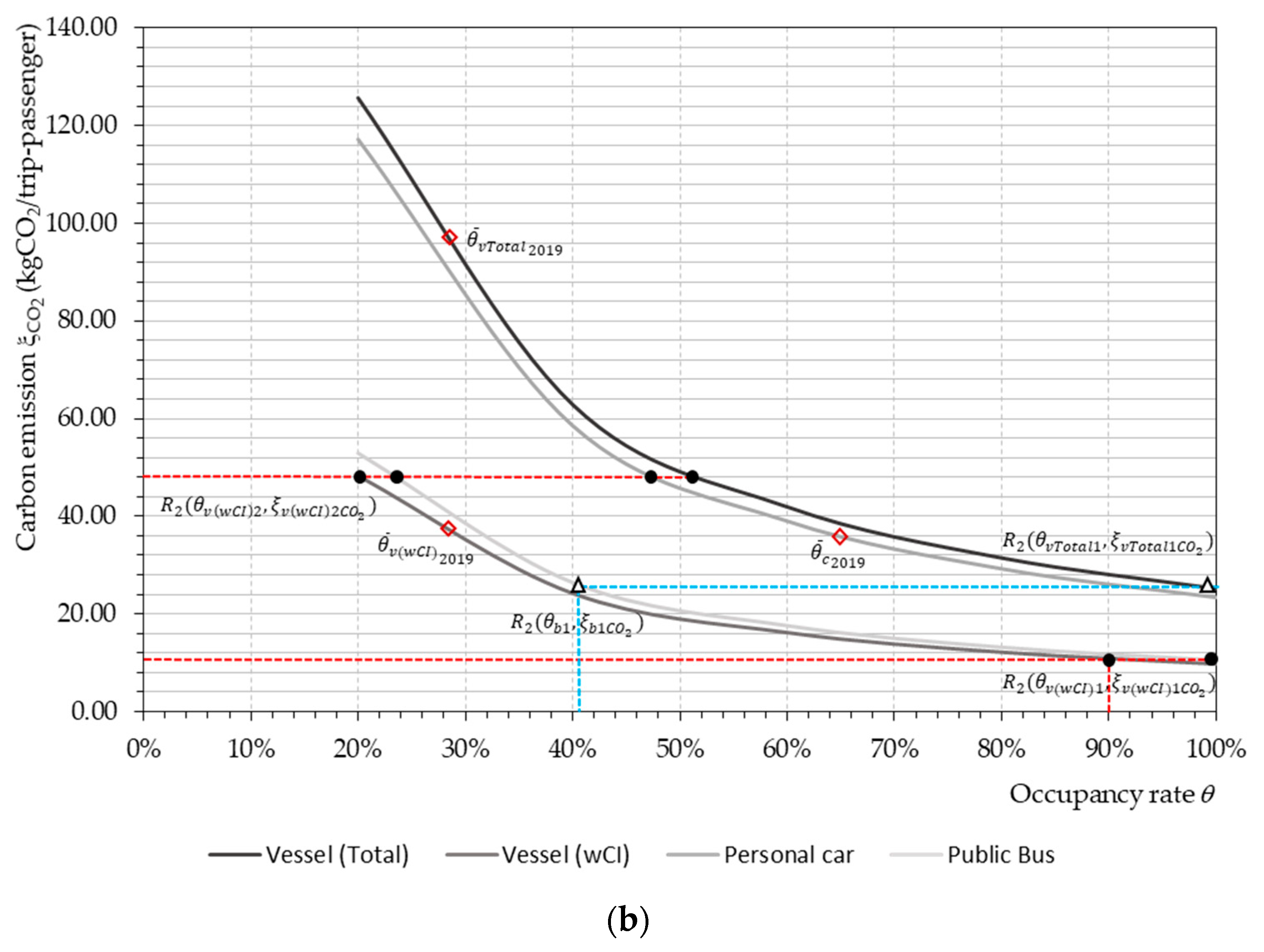
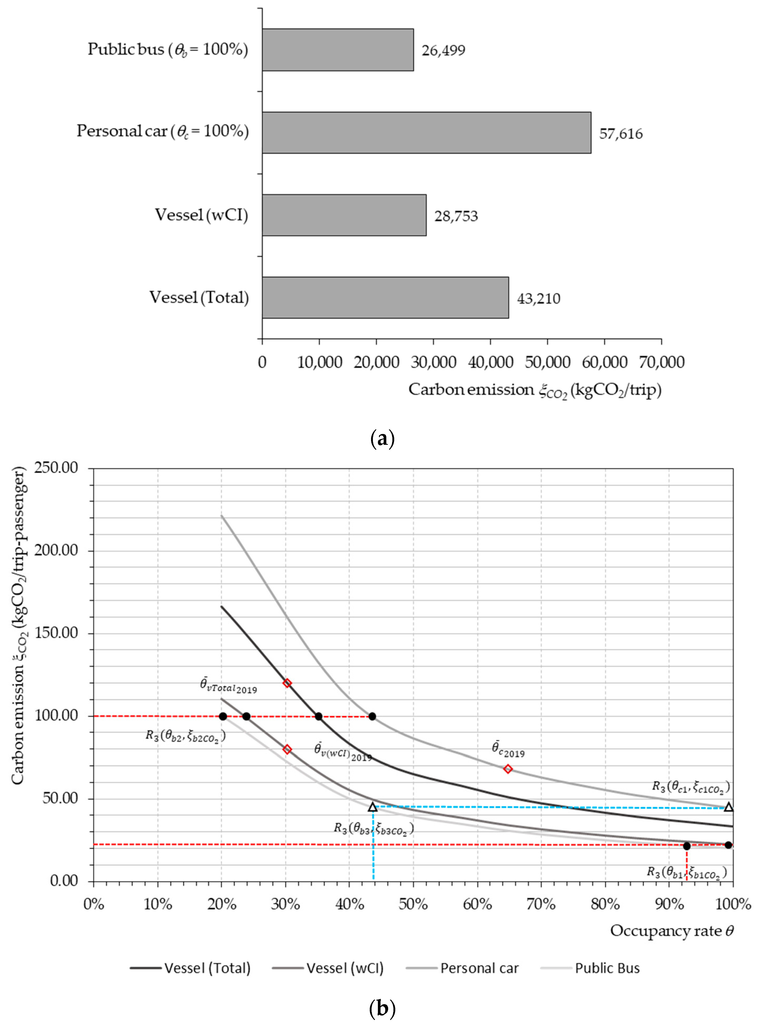
4. Results and Discussion
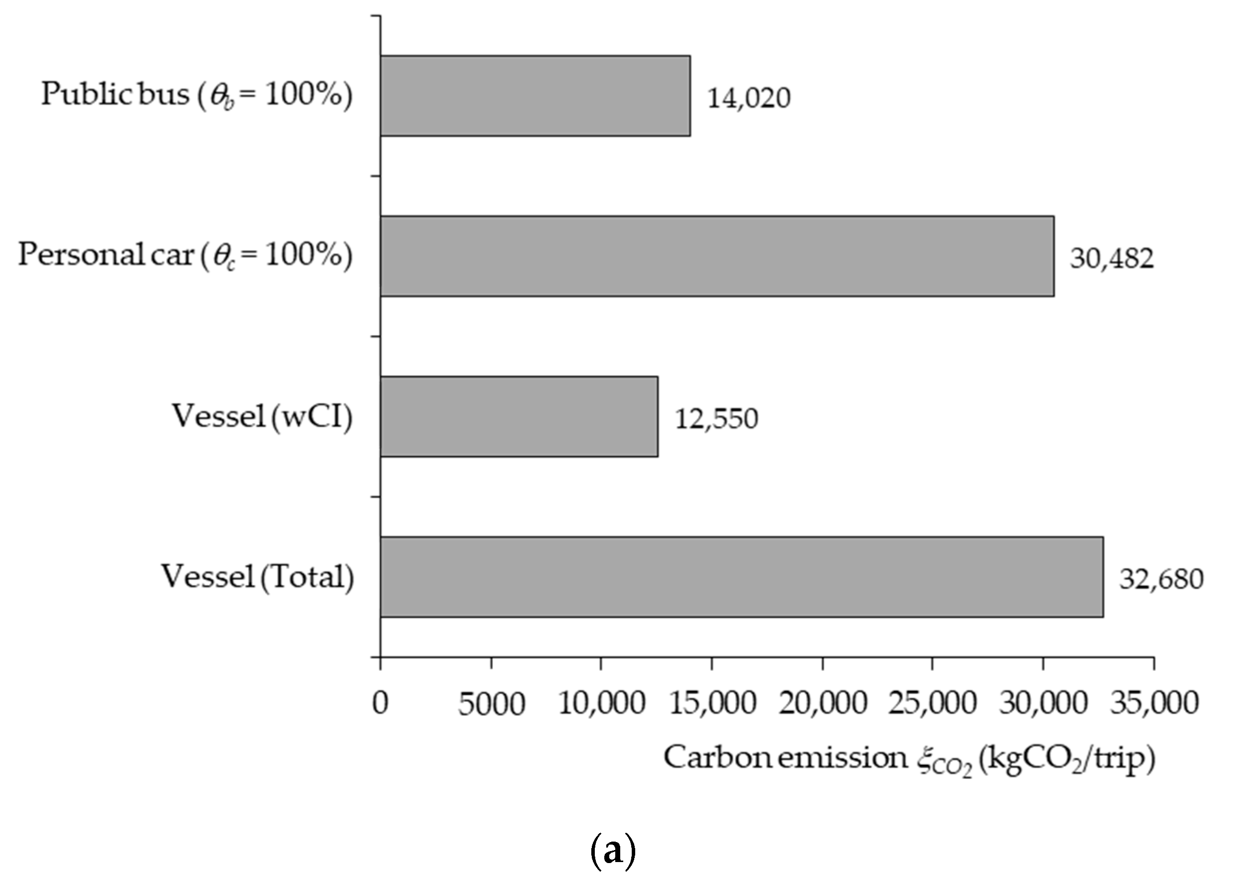
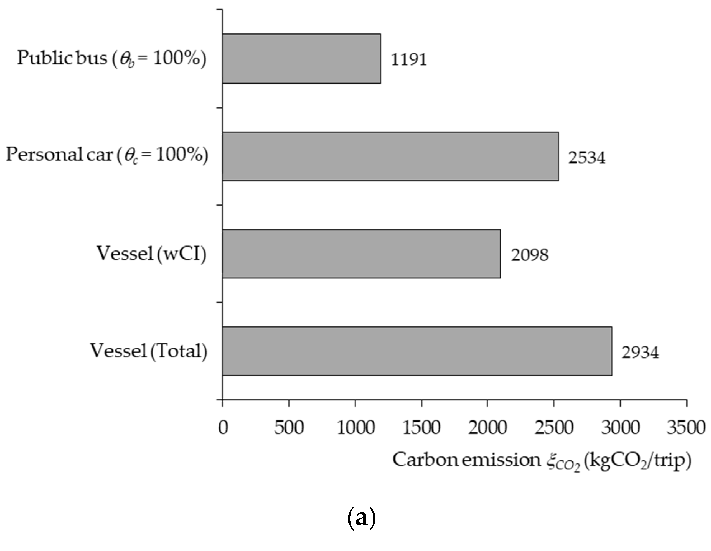
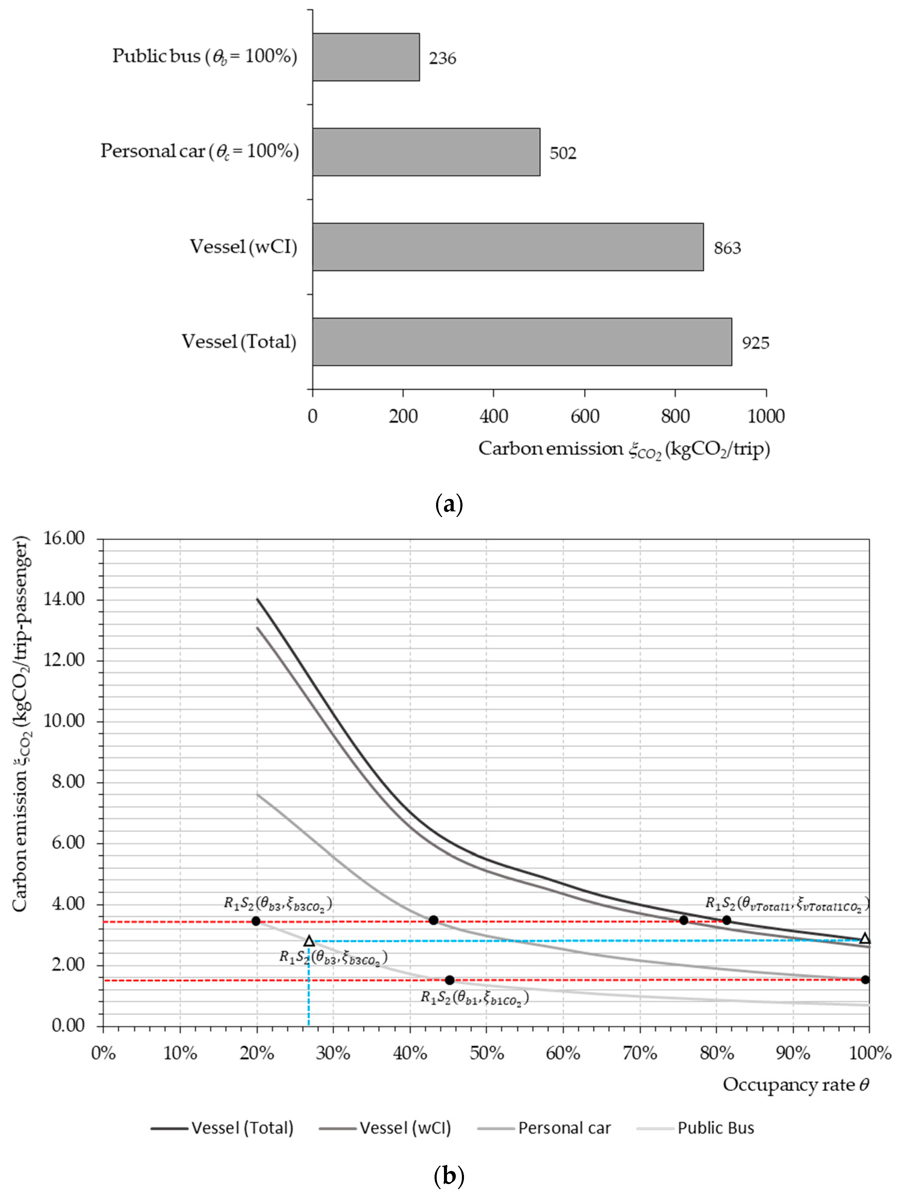
- The total carbon emission for each transportation mode based on the reference capacity;
- The calculated carbon emission values per passenger considering different transportation modes;
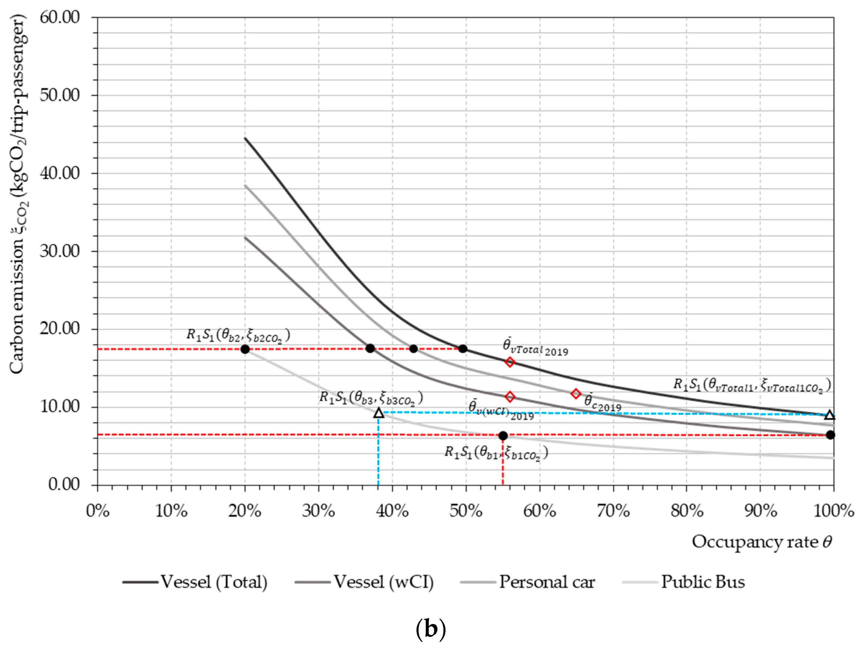
- The optimal transportation mode choice with respect to the different relative occupancy rates;
- The calculated carbon emission relationship for available actual observed occupancy rates.
4.1. Case Study 1—Venice–Pula–Poreč–Venice ()
4.1.1. Route Segment Venice–Pula ()
4.1.2. Route Segment Pula–Poreč ()
4.1.3. Route Segment Poreč–Venice ()
4.2. Case Study 2—Ancona–Zadar ()
4.3. Case Study 3—Dubrovnik–Bari ()
4.4. Discussion
5. Conclusions
Author Contributions
Funding
Institutional Review Board Statement
Informed Consent Statement
Data Availability Statement
Acknowledgments
Conflicts of Interest
References
- European Environment Agency (EEA). Greenhouse Gas Emissions from Transport in Europe. Available online: https://www.eea.europa.eu/ims/greenhouse-gas-emissions-from-transport (accessed on 6 February 2022).
- European Environment Agency (EEA). Share of Transport Greenhouse Gas Emissions. Available online: https://www.eea.europa.eu/data-and-maps/daviz/share-of-transport-ghg-emissions-2/#tab-googlechartid_chart_13 (accessed on 6 February 2022).
- European Environment Agency (EEA). Passenger and Freight Transport Demand in Europe. Available online: https://www.eea.europa.eu/data-and-maps/indicators/passenger-and-freight-transport-demand/assessment-1 (accessed on 6 February 2022).
- Croatian Bureau of Statistics. Available online: https://www.dzs.hr/default_e.htm (accessed on 15 November 2021).
- European Environment Agency (EEA). Rail and Waterborne—Best for Low-Carbon Motorised Transport. Available online: https://www.eea.europa.eu/publications/rail-and-waterborne-transport (accessed on 2 December 2021).
- International Maritime Organization (IMO). Guidelines for Voluntary Use of the Ship Energy Efficiency Operational Indicator (EEOI). MPEC.1/Circ.684. Available online: https://wwwcdn.imo.org/localresources/en/OurWork/Environment/Documents/Circ-684.pdf (accessed on 2 December 2021).
- International Maritime Organization (IMO). Guidelines on Survey and Certification of the Energy Efficiency Design Index (EEDI), as Amended (Resolution MEPC.254(67), as Amended by Resolution MEPC.261(68) and Resolution MEPC.309(73)). MPEC.1/Circ.855/Rev.2. Available online: https://wwwcdn.imo.org/localresources/en/OurWork/Environment/Documents/MEPC.1-Circ.855-Rev.2.pdf (accessed on 2 December 2021).
- Mannarini, G.; Carelli, L.; Orović, J.; Martinkus, C.P.; Coppini, G. Towards Least-CO2 Ferry Routes in the Adriatic Sea. J. Mar. Sci. Eng. 2021, 9, 115. [Google Scholar] [CrossRef]
- Dagkinis, I.; Nikitakos, N. Slow Steaming Options Investigation Using Multi Criteria Decision Analysis Method. In Proceedings of the Conference ECONSHIP2015, Chios, Greece, 24–27 June 2015. [Google Scholar]
- Department for Environment, Food and Rural Affairs (DEFRA). Passenger Transport Emission Factors—Methodology Factor. Available online: https://www.carbonindependent.org/files/passenger-transport.pdf (accessed on 17 November 2021).
- Ančić, I.; Perčić, M.; Vladimir, N. Alternative Power Options to Reduce Carbon Footprint of Ro-Ro Passenger Fleet: A Case Study of Croatia. J. Clean. Prod. 2020, 271, 122638. [Google Scholar] [CrossRef]
- Rešetar, M.; Pejić, G.; Lulic, Z. Road Transport Emissions of Passenger Cars in the Republic of Croatia. In Proceedings of the 8th European Combustion Meeting, Dubrovnik, Croatia, 18–21 April 2017. [Google Scholar]
- European Commission (EC). A Clean Planet for All—A European Strategic Long-Term Vision for a Prosperous, Modern, Competitive and Climate Neutral Economy. COM(2018) 773 Final. Available online: https://eur-lex.europa.eu/legal-content/EN/TXT/PDF/?uri=CELEX:52018DC0773 (accessed on 21 November 2021).
- European Parliament. Maritime Transport: Strategic Approach. Available online: https://www.europarl.europa.eu/factsheets/en/sheet/124/maritime-transport-strategic-approach (accessed on 21 November 2021).
- European Parliament. Integrated Maritime Policy of the European Union. Available online: https://www.europarl.europa.eu/factsheets/en/sheet/121/integrated-maritime-policy-of-the-european-union (accessed on 21 November 2021).
- European Commission (EC). Roadmap to a Single European Transport Area—Towards a Competitive and Resource Efficient Transport System. White Paper. COM(2011—144 Final). Available online: https://eur-lex.europa.eu/LexUriServ/LexUriServ.do?uri=COM:2011:0144:FIN:EN:PDF (accessed on 21 November 2021).
- European Commission (EC). Strategic Goals and Recommendations for the EU’s Maritime Transport Policy until 2018. COM (2009-8 Final). Available online: https://eur-lex.europa.eu/LexUriServ/LexUriServ.do?uri=COM%3A2009%3A0008%3AFIN%3AEN%3APDF (accessed on 21 November 2021).
- European Commission (EC). The European Green Deal. COM (2019—640 Final). Available online: https://eur-lex.europa.eu/legal-content/EN/TXT/?uri=COM%3A2019%3A640%3AFIN (accessed on 21 November 2021).
- European Commission (EC). Sustainable and Smart Mobility Strategy. (COM/2020/789 Final). Available online: https://eur-lex.europa.eu/legal-content/EN/TXT/?uri=CELEX%3A52020DC0789 (accessed on 21 November 2021).
- Kane, L.; Del Mistro, R. Changes in Transport Planning Policy: Changes in Transport Planning Methodology? Transportation 2003, 30, 113–131. [Google Scholar] [CrossRef]
- Zuidgeest, M.; Maarseveen, M.F.A.M. Transportation Planning for Sustainable Development. In Proceedings of the 19th South African Transport Conference (SATC 2000), Pretoria, South Africa, 17–20 July 2000. [Google Scholar]
- Litman, T. Introduction to Multi-Modal Transportation Planning; Victoria Transport Policy Institute: Victoria, BC, Canada, 2017. [Google Scholar]
- Sirotić, M.; Žuškin, S.; Rudan, I.; Stocchetti, A. Methodology for the Sustainable Development of the Italy-Croatia Cross-Border Area: Sustainable and Multimodal/Cross-Border Passenger Services. Sustainability 2021, 13, 11895. [Google Scholar] [CrossRef]
- Wiedmann, T.; Minx, J. A Definition of ‘Carbon Footprint’. In Ecological Economics Research Trends; Nova Science Publishers: Hauppauge, NY, USA, 2008; pp. 1–11. [Google Scholar]
- Pandey, D.; Agrawal, M.; Pandey, J.S. Carbon Footprint: Current Methods of Estimation. Environ. Monit. Assess. 2011, 178, 135–160. [Google Scholar] [CrossRef]
- Sarkodie, S.A. Environmental Performance, Biocapacity, Carbon & Ecological Footprint of Nations: Drivers, Trends and Mitigation Options. Sci. Total Environ. 2021, 751, 141912. [Google Scholar] [CrossRef]
- Lenzen, M.; Sun, Y.-Y.; Faturay, F.; Ting, Y.-P.; Geschke, A.; Malik, A. The Carbon Footprint of Global Tourism. Nat. Clim. Change 2018, 8, 522–528. [Google Scholar] [CrossRef]
- Osorio-Tejada, J.L.; Llera-Sastresa, E.; Hariza Hashim, A. Well-to-Wheels Approach for the Environmental Impact Assessment of Road Freight Services. Sustainability 2018, 10, 4487. [Google Scholar] [CrossRef] [Green Version]
- Ma, F.; Wang, W.; Sun, Q.; Liu, F.; Li, X. Ecological Pressure of Carbon Footprint in Passenger Transport: Spatio-Temporal Changes and Regional Disparities. Sustainability 2018, 10, 317. [Google Scholar] [CrossRef] [Green Version]
- Kitamura, Y.; Ichisugi, Y.; Karkour, S.; Itsubo, N. Carbon Footprint Evaluation Based on Tourist Consumption toward Sustainable Tourism in Japan. Sustainability 2020, 12, 2219. [Google Scholar] [CrossRef] [Green Version]
- Wang, S.; Ge, M. Everything You Need to Know About the Fastest-Growing Source of Global Emissions: Transport; World Resources Institute: Washington, DC, USA, 2019. [Google Scholar]
- Ülker, D.; Bayırhan, İ.; Mersin, K.; Gazioğlu, C. A Comparative CO2 Emissions Analysis and Mitigation Strategies of Short-Sea Shipping and Road Transport in the Marmara Region. Carbon Manag. 2021, 12, 1–12. [Google Scholar] [CrossRef]
- Yang, L.; Zhang, Q.; Zhang, Y.; Lv, Z.; Wang, Y.; Wu, L.; Feng, X.; Mao, H. An AIS-Based Emission Inventory and the Impact on Air Quality in Tianjin Port Based on Localized Emission Factors. Sci. Total Environ. 2021, 783, 146869. [Google Scholar] [CrossRef] [PubMed]
- Zhang, S.; Peng, D.; Li, Y.; Zu, L.; Fu, M.; Yin, H.; Ding, Y. Study on the Real-World Emissions of Rural Vehicles on Different Road Types. Environ. Pollut. 2021, 273, 116453. [Google Scholar] [CrossRef] [PubMed]
- Sun, Z.; Wang, C.; Ye, Z.; Bi, H. Long Short-Term Memory Network-Based Emission Models for Conventional and New Energy Buses. Int. J. Sustain. Transp. 2021, 15, 229–238. [Google Scholar] [CrossRef]
- Angelevska, B.; Atanasova, V.; Andreevski, I. Urban Air Quality Guidance Based on Measures Categorization in Road Transport. Civ. Eng. J. 2021, 7, 253–267. [Google Scholar] [CrossRef]
- Obaid, M.; Torok, A.; Ortega, J. A Comprehensive Emissions Model Combining Autonomous Vehicles with Park and Ride and Electric Vehicle Transportation Policies. Sustainability 2021, 13, 4653. [Google Scholar] [CrossRef]
- Batur, İ.; Bayram, I.S.; Koc, M. Impact Assessment of Supply-Side and Demand-Side Policies on Energy Consumption and CO2 Emissions from Urban Passenger Transportation: The Case of Istanbul. J. Clean. Prod. 2019, 219, 391–410. [Google Scholar] [CrossRef] [Green Version]
- Zhang, H.; Razzaq, A.; Pelit, I.; Irmak, E. Does Freight and Passenger Transportation Industries Are Sustainable in BRICS Countries? Evidence from Advance Panel Estimations. Econ. Res.—Ekonomska Istraživanja 2021, 0:0, 1–21. [Google Scholar] [CrossRef]
- Brewer, T.L. Black Carbon Emissions and Regulatory Policies in Transportation. Energy Policy 2019, 129, 1047–1055. [Google Scholar] [CrossRef]
- Fridell, E.; Bäckström, S.; Stripple, H. Considering Infrastructure When Calculating Emissions for Freight Transportation. Transp. Res. Part D Transp. Environ. 2019, 69, 346–363. [Google Scholar] [CrossRef]
- Anenberg, S.; Miller, J.; Henze, D.; Minjares, R. A Global Snapshot of the Air Pollution-Related Health Impacts of Transportation Sector Emissions in 2010 and 2015; International Council on Clean Transportation: Washington, DC, USA, 2019. [Google Scholar]
- Russo, M.A.; Relvas, H.; Gama, C.; Lopes, M.; Borrego, C.; Rodrigues, V.; Robaina, M.; Madaleno, M.; Carneiro, M.J.; Eusébio, C.; et al. Estimating Emissions from Tourism Activities. Atmos. Environ. 2020, 220, 117048. [Google Scholar] [CrossRef]
- Wang, S.; Psaraftis, H.N.; Qi, J. Paradox of International Maritime Organization’s Carbon Intensity Indicator. Commun. Transp. Res. 2021, 1, 100005. [Google Scholar] [CrossRef]
- Skrúcaný, T.; Kendra, M.; Kalina, T.; Jurkovič, M.; Vojtek, M.; Synák, F. Environmental Comparison of Different Transport Modes. NAŠE MORE 2018, 65, 192–196. [Google Scholar] [CrossRef]
- Rivarolo, M.; Iester, F.; Massardo, A.F. An Algorithm for Comparative Analysis of Power and Storage Systems for Maritime Applications. E3S Web Conf. 2022, 334, 06001. [Google Scholar] [CrossRef]
- Wanke, P.; Chen, Z.; Zheng, X.; Antunes, J. Sustainability Efficiency and Carbon Inequality of the Chinese Transportation System: A Robust Bayesian Stochastic Frontier Analysis. J. Environ. Manag. 2020, 260, 110163. [Google Scholar] [CrossRef]
- Fridell, E. Emissions and Fuel Use in the Shipping Sector. In Green Ports: Inland and Seaside Sustainable Transportation Strategies; Bergqvist, R., Monios, J., Eds.; Elsevier: Amsterdam, The Netherlands, 2019; pp. 19–33. ISBN 978-0-12-814054-3. [Google Scholar]
- Zis, T.P.V.; Psaraftis, H.N.; Tillig, F.; Ringsberg, J.W. Decarbonizing Maritime Transport: A Ro-Pax Case Study. Res. Transp. Bus. Manag. 2020, 37, 100565. [Google Scholar] [CrossRef]
- Kang, A.S.; Jayaraman, K.; Soh, K.-L.; Wong, W.-P. Tackling Single-Occupancy Vehicles to Reduce Carbon Emissions: Actionable Model of Drivers’ Implementation Intention to Try Public Buses. J. Clean. Prod. 2020, 260, 121111. [Google Scholar] [CrossRef]
- Shiraki, H.; Matsumoto, K.; Shigetomi, Y.; Ehara, T.; Ochi, Y.; Ogawa, Y. Factors Affecting CO2 Emissions from Private Automobiles in Japan: The Impact of Vehicle Occupancy. Appl. Energy 2020, 259, 114196. [Google Scholar] [CrossRef]
- Soukhov, A.; Mohamed, M. Occupancy and GHG Emissions: Thresholds for Disruptive Transportation Modes and Emerging Technologies. Transp. Res. Part D Transp. Environ. 2022, 102, 103127. [Google Scholar] [CrossRef]
- Amatuni, L.; Ottelin, J.; Steubing, B.; Mogollón, J.M. Does Car Sharing Reduce Greenhouse Gas Emissions? Assessing the Modal Shift and Lifetime Shift Rebound Effects from a Life Cycle Perspective. J. Clean. Prod. 2020, 266, 121869. [Google Scholar] [CrossRef]
- Fernando, C.; Soo, V.K.; Compston, P.; Doolan, M. The Impact of Car-Based Shared Mobility on Greenhouse Gas Emissions: A Review; Social Science Research Network: Rochester, NY, USA, 2022. [Google Scholar]
- Chergui, S.; Agoujil, S. Implementation of Vehicle Occupancy and Aggregate Emission Rate. In Proceedings of the 3rd International Conference on Smart City Applications, Tetouan, Morocco, 10–11 October 2018; Association for Computing Machinery: New York, NY, USA, 2018; pp. 1–5. [Google Scholar]
- Schembari, C.; Cavalli, F.; Cuccia, E.; Hjorth, J.; Calzolai, G.; Pérez, N.; Pey, J.; Prati, P.; Raes, F. Impact of a European Directive on Ship Emissions on Air Quality in Mediterranean Harbours. Atmos. Environ. 2012, 61, 661–669. [Google Scholar] [CrossRef]
- Pseftogkas, A.; Koukouli, M.-E.; Skoulidou, I.; Balis, D.; Meleti, C.; Stavrakou, T.; Falco, L.; van Geffen, J.; Eskes, H.; Segers, A.; et al. A New Separation Methodology for the Maritime Sector Emissions over the Mediterranean and Black Sea Regions. Atmosphere 2021, 12, 1478. [Google Scholar] [CrossRef]
- Stazić, L.; Radonja, R.; Pelić, V.; Lalić, B. The Port of Split International Marine Traffic Emissions Inventory. Pomorstvo 2020, 34, 32–39. [Google Scholar] [CrossRef]
- Škurić, M.; Maraš, V.; Radonjic, A.; Gagić, R.; Nikolić, D. Some Results of Air Pollution from Passenger Ferries in the Boka Kotorska Bay. In The Montenegrin Adriatic Coast; The Handbook of Environmental Chemistry; Springer International Publishing: Cham, Switzerland, 2021; ISBN 978-3-030-77628-2. [Google Scholar]
- Vidas, S.; Cukrov, M.; Šutalo, V.; Rudan, S. CO2 Emissions Reduction Measures for RO-RO Vessels on Non-Profitable Coastal Liner Passenger Transport. Sustainability 2021, 13, 6909. [Google Scholar] [CrossRef]
- Degiuli, N.; Martić, I.; Farkas, A.; Gospić, I. The Impact of Slow Steaming on Reducing CO2 Emissions in the Mediterranean Sea. Energy Rep. 2021, 7, 8131–8141. [Google Scholar] [CrossRef]
- Merico, E.; Gambaro, A.; Argiriou, A.; Alebic-Juretic, A.; Barbaro, E.; Cesari, D.; Chasapidis, L.; Dimopoulos, S.; Dinoi, A.; Donateo, A.; et al. Atmospheric Impact of Ship Traffic in Four Adriatic-Ionian Port-Cities: Comparison and Harmonization of Different Approaches. Transp. Res. Part D Transp. Environ. 2017, 50, 431–445. [Google Scholar] [CrossRef]
- ISO 8217 2017; Fuel Standard for Marine Distillate Fuel. World Fuel Services Corporation: Miami, FL, USA, 2017. Available online: https://www.wfscorp.com/sites/default/files/ISO-8217-2017-Tables-1-and-2-1-1.pdf (accessed on 5 November 2021).
- Trivyza, N.L.; Rentizelas, A.; Theotokatos, G. A Comparative Analysis of EEDI Versus Lifetime CO2 Emissions. J. Mar. Sci. Eng. 2020, 8, 61. [Google Scholar] [CrossRef] [Green Version]
- Tran, T.A. Calculation and Assessing the EEDI Index in the Field of Ship Energy Efficiency for M/V Jules Garnier. J Mar. Sci Res Dev 2016, 6, 212. [Google Scholar] [CrossRef] [Green Version]
- Babicz, J. Wartsila Encyclopedia of Ship Technology, 2nd ed.; WÄRTSILÄ Corporation: Helsinki, Finland, 2015. [Google Scholar]
- Waters, J. Atlantic Center for the Innovative Design and Control of Small Ships: Surface Effect Ship (Ses) Test Program. In Proceedings of the 2004 American Society for Engineering Education Annual Conference & Exposition, Salt Lake City, UT, USA, 20–23 June 2004; pp. 9.242.1–9.242.10. [Google Scholar]
- Ančić, I.; Vladimir, N.; Cho, D.-S. Determining Environmental Pollution from Ships Using Index of Energy Efficiency and Environmental Eligibility (I4E). Mar. Policy 2018, 95, 1–7. [Google Scholar] [CrossRef]
- Finnish Information Centre of Automobile Sector (Autoalan Tiedotuskeskus). ACEA Statistics. Average Age of Passenger Cars in European Countries. Available online: https://www.aut.fi/en/statistics/international_statistics/average_age_of_passenger_cars_in_european_countries (accessed on 15 November 2021).
- European Environment Agency (EEA). Average CO2 Emissions from Newly Registered Motor Vehicles in Europe. Available online: https://www.eea.europa.eu/data-and-maps/indicators/average-co2-emissions-from-motor-vehicles/assessment-1 (accessed on 2 December 2021).
- Interreg Italy-Croatia Maritime and Multimodal Sustainable Passenger Transport and Services (MIMOSA). O.3.5. Cross-Border Transport Sustainability Action Plan. Available online: https://edu.pfri.hr/mimosa/ (accessed on 5 January 2022).
- MarineTraffic: Global Ship Tracking Intelligence. Available online: https://www.marinetraffic.com/en/ais/home/centerx:-12.0/centery:25.0/zoom:4 (accessed on 23 December 2021).
- EMSA\THETIS-MRV. Available online: https://mrv.emsa.europa.eu/#public/eumrv (accessed on 17 January 2022).


| Vessel Operation | Time Period | Relative Period |
|---|---|---|
| ) | ||
| ) | ||
| ) | ||
| Northern Adriatic Region | Middle Adriatic Region | Southern Adriatic Region |
|---|---|---|
| Pesaro–Mali Lošinj | Split–Ancona | Dubrovnik–Bari |
| Rab–Cesenatico | Ancona–Zadar | |
| Pesaro–Zadar | Civitanova–Hvar | |
| Poreč–Venice | Civitanova–Split | |
| Venice–Pula | ||
| Pula–Trieste | ||
| Rovinj–Venice | ||
| Rovinj–Cesenatico | ||
| Trieste–Piran–Rovinj | ||
| Pula–Venice |
| Passenger Lines (Line Operator) | Vessel Name | Average Passenger Occupancy per Trip in 2019 | Number of Vessel Voyages in 2019 |
|---|---|---|---|
| Pula–Venice (Venezia Lines LTD) | San Pawl | 56% | 44 |
| Poreč–Venice (Venezia Lines LTD) | San Pawl | 30.6% | 88 |
| Technical Characteristics: Vessel “San Pawl” | |
|---|---|
| Vessel type | HSC air cushion |
| Summer DWT | 50 t |
| Length overall (LOA) | 35.3 m |
| Breadth | 11.5 m |
| Draught | 2.05 m |
| Propulsion type | 2× fixed pitch propellers |
| Propulsion power | 3358 kW |
| Maritime Transportation Mode Distances (Nm) | Road Transportation Mode Distances (km) | ||||
|---|---|---|---|---|---|
| Route Segment | Maneuvering | Sea Passage | Total | Road | Total |
| 12.7 | 63.5 | 76.2 | 283 | 283 | |
| 3.8 | 26.6 | 30.4 | 56 | 56 | |
| 10.7 | 50 | 60.7 | 250 | 250 | |
| Maneuvering on departure | 9.8 Nm |
| Sea passage | 63.5 Nm |
| Maneuvering on arrival | 2.9 Nm |
| Maneuvering on departure | 2.9 Nm |
| Sea passage | 26.6 Nm |
| Maneuvering on arrival | 0.9 Nm |
| Maneuvering on departure | 0.9 Nm |
| Sea passage | 50 Nm |
| Maneuvering on arrival | 9.8 Nm |
| Passenger Line (Line Operator) | Vessel Name | Average Passenger Occupancy per Trip in 2019 | Number of Vessel Voyages in 2019 |
|---|---|---|---|
| Ancona–Zadar (Jadrolinija) | Zadar | 28.5% | 49 |
| Technical Characteristics: Vessel “Zadar” | |
|---|---|
| Vessel type | RO-PAX ferry |
| Summer DWT | 2152 t |
| Length over all (LOA) | 116 m |
| Breadth | 18.9 m |
| Draught | 5.15 m |
| Propulsion type | 2× controllable pitch propellers |
| Propulsion power | 7.000 kW |
| Maritime Transportation Mode Distances (Nm) | Road Transportation Mode Distances (km) | ||||
|---|---|---|---|---|---|
| Route | Maneuvering | Sea Passage | Total | Road | Total |
| R2 | 6.7 | 84.7 | 91.4 | 864 | 864 |
| Maneuvering on departure | 4.2 Nm |
| Sea passage | 84.7 Nm |
| Maneuvering on arrival | 2.5 Nm |
| Passenger Line (Line Operator) | Vessel Name | Average Passenger Occupancy per Trip in 2019 | Number of Vessel Voyages in 2019 |
|---|---|---|---|
| Dubrovnik–Bari (Jadrolinija) | Dubrovnik | 30.5% | 87 voyages |
| Technical Characteristics: Vessel “Dubrovnik” | |
|---|---|
| Vessel type | RO-PAX Ferry |
| Summer DWT | 1310 t |
| Length over all (LOA) | 113.01 m |
| Breadth | 18.5 m |
| Draught | 4.83 m |
| Propulsion type | 2× controllable pitch propellers |
| Propulsion power | 13,248 kW |
| Maritime Transportation Mode Distances (Nm) | Road Transportation Mode Distances (km) | ||||
|---|---|---|---|---|---|
| Route | Maneuvering | Sea Passage | Total | Road | Total |
| 4.5 | 104.4 | 108.9 | 1633 | 1633 | |
| Maneuvering on departure | 2.1 Nm |
| Sea passage | 104.4 Nm |
| Maneuvering on arrival | 2.4 Nm |
| 2933.7 | 924.5 | 2346.5 | 32,680.2 | 43,210.4 | |
| 2098.1 | 862.7 | 1281.1 | 12,549.8 | 28,752.5 | |
| 38.4 | 7.6 | 33.93 | 117.24 | 221.6 | |
| 170.08 | 33.66 | 150.25 | 519.26 | 981.43 |
| 1714.3 | 712.9 | 965.9 | 7801.1 | 19,765.2 | |
| 383.8 | 149.8 | 315.2 | 4748.7 | 8987.3 | |
| 2098.1 | 862.7 | 1281.1 | 12,549.8 | 28,752.5 |
Publisher’s Note: MDPI stays neutral with regard to jurisdictional claims in published maps and institutional affiliations. |
© 2022 by the authors. Licensee MDPI, Basel, Switzerland. This article is an open access article distributed under the terms and conditions of the Creative Commons Attribution (CC BY) license (https://creativecommons.org/licenses/by/4.0/).
Share and Cite
Dujmović, J.; Krljan, T.; Lopac, N.; Žuškin, S. Emphasis on Occupancy Rates in Carbon Emission Comparison for Maritime and Road Passenger Transportation Modes. J. Mar. Sci. Eng. 2022, 10, 459. https://doi.org/10.3390/jmse10040459
Dujmović J, Krljan T, Lopac N, Žuškin S. Emphasis on Occupancy Rates in Carbon Emission Comparison for Maritime and Road Passenger Transportation Modes. Journal of Marine Science and Engineering. 2022; 10(4):459. https://doi.org/10.3390/jmse10040459
Chicago/Turabian StyleDujmović, Josip, Tomislav Krljan, Nikola Lopac, and Srđan Žuškin. 2022. "Emphasis on Occupancy Rates in Carbon Emission Comparison for Maritime and Road Passenger Transportation Modes" Journal of Marine Science and Engineering 10, no. 4: 459. https://doi.org/10.3390/jmse10040459
APA StyleDujmović, J., Krljan, T., Lopac, N., & Žuškin, S. (2022). Emphasis on Occupancy Rates in Carbon Emission Comparison for Maritime and Road Passenger Transportation Modes. Journal of Marine Science and Engineering, 10(4), 459. https://doi.org/10.3390/jmse10040459