An Original Vibrodiagnostic Device to Control Linear Rolling Conveyor Reliability

Abstract

On the basis of an analysis of the number of goods that are transported and handled in maritime transport, the ports for cargo ships may be considered as places with concentrated emissions. Reducing the emissions in ports can be achieved by shortening the stay times of cargo ships. The time that ships spend in ports may be reduced to the time that is required for the effective handling of the goods. One of the solutions for effective handling is using equipment with linear rolling systems. To prevent the idle time of cargo ships and the unnecessary increment of emissions in ports because of the possible failure of the linear rolling systems, their reliability and failure prediction are greatly required. Unfortunately, the common diagnostic systems of linear rolling systems in transportation practice still fail in particular cases of great external loads. Therefore, an original solution of the diagnostic system was designed on the basis of a load-free diagnostic part with a vibration sensor that is integrated into a carriage of the linear rolling system. A functional sample of the diagnostics was produced, and the vibrations that were measured on a loaded carriage and on the diagnostic part were compared in laboratory conditions under significant external loads. Encouraging results were reached by a time-domain analysis of the measured data. On the diagnostic part, the damage appeared clearly, while, on the loaded carriage, there were no observable signs of damage.

1. Introduction

Because of significant climate change, which is increasing GHG (greenhouse gas) emissions and global warming, the sustainability of maritime transport is currently in demand. As maritime transport creates 80% of the global transportation of goods, the necessity of decreasing the emissions that are related to container and other cargo ships is obvious. The United Nations [1,2] mentions that, for the effective reduction in the GHG emissions in maritime transport, improvements in the port logistics should be included.

Ports can optimise and ensure the availability of the berth at the moment when ships arrive in order to avoid idle time that leads to an unnecessary increment of the emissions in ports [3,4,5,6]. Logistics problems by berthing containers and cargo ships may be caused by insufficient communication between the ports and the ships, as well as by internal logistics challenges that are connected with the unloading/loading of goods, or with the transportation of goods within the port [7,8,9,10].

Especially in the case of internal transportation, the manipulation and positioning of containers and goods, which are requirements in logistics operations, are increasing so that the processes will be fast, effective, and reliable. To secure this assumption, increased attention must be paid to the reliability and failure prediction of the crane subcomponents and their positioning, and of the clamping systems and handling machines. In transportation practice, linear rolling systems that realise the linear motion of these machines and that are the basis of their design, are said to be critical [11,12,13,14,15]. Their failure may lead to the breakdown of the machine, the collapse of the logistic chain, and, thus, to an increase in the emissions that are produced by the ships that are waiting for the berth. Therefore, special emphasis is given to the diagnostics and failure prediction of the linear rolling systems that are used in port logistics.

The diagnostics of linear rolling systems is based on the knowledge of rolling bearing diagnostics. In the diagnostics of rolling bearings, the methods usually aim to measure the vibrations or the acoustic emissions. However, the transition from bearing diagnostics to the diagnostics of linear rolling systems is not so simple. Japanese producer, THK (THK Co., Ltd., Tokyo, Japan), in the patent [16], mention that the design of linear systems might negatively influence the diagnostics on the basis of the measurement of the vibrations or the noise intensity. The transition of the rolling elements from a nonloaded state to a loaded one excites vibrations that are similar to those created by the damage of the guiding profile in the time domain. In the frequency domain, the signal that belongs to the changed status shows a frequency that is identical to the guiding profile damage.

Therefore, researchers and the producers of linear rolling systems developed diagnostic systems that are based on measuring the acceleration of the vibrations, and on interpreting the measured vibrations through the RMS (root mean square) values, a spectral analysis, and the crest factor [17], or a spectrogram [18,19], in the context of the lubrication level, which provides the reference value of the RMS. Feng [20] explains the influence of lubrication on the RMS and its distribution in the frequency domain. He detected an increased RMS in a high-frequency band by progressing damage.

The producer of THK, in its patent [21], argues for the use of an acceleration sensor for measuring the vibrations, and for the use of a presence sensor of the rolling elements to determine the actual velocity of the linear system. The vibrations are evaluated through the RMS values in the high-frequency band, which reflect the lubrication level and the linear system velocity. When the experimentally determined limit value is exceeded, the linear system is relubricated, and the level of the vibrations is measured again.

The producer, Schaeffler (Schaeffler Technologies AG & Co. KG, Herzogenaurach, Germany), brought in a similar method of diagnostics [22] that uses the acceleration sensor for measuring vibrations. The measured vibrations are evaluated through the RMS values in the high-frequency band from 14 kHz to 25 kHz. When the limit value is exceeded, the linear system is relubricated. A decisive quantity is the time of a relubricating process compared to the experimentally given distribution function of the linear system life. The analysing procedure is processed through neural networks.

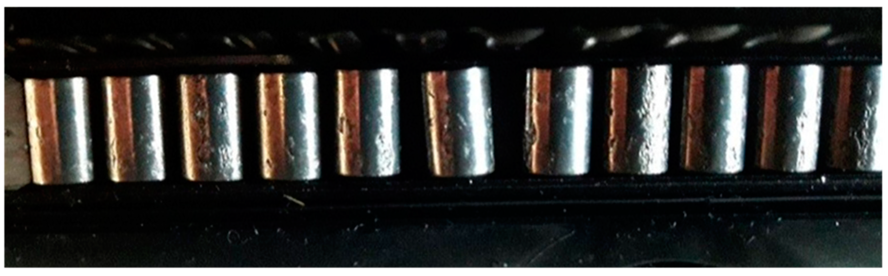
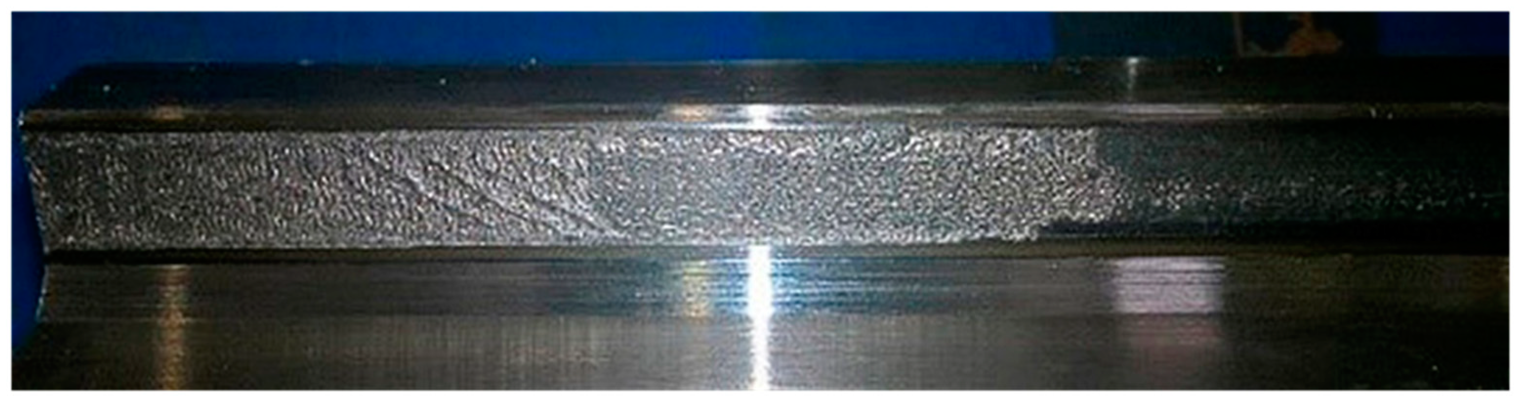
Unfortunately, the diagnostics of linear rolling systems that are currently provided by producers still do not appear reliable enough in transportation practice. In practice, several cases of significant damage to the guiding profiles (Figure 1) and the rolling elements (Figure 2) may be noticed. In these cases, the linear rolling systems were operated under significant external loads by the weight of the transported goods. The measured vibrations did not exceed the threshold value, and the linear systems were considered serviceable according to the vibrodiagnostics that was used. Thus, the paper aims to describe the development of an original principle for linear rolling system diagnostics.

2. Materials and Methods

In the specific case of handling machines, linear rolling systems are frequently operated under enormous loads. These loads are related to the mass inertia of the connected mechanical assemblies and of the transported goods. The mass inertia causes a dynamical load that is composed of static and dynamical forces. In this context, it may be noticed that the dynamical character of the load negatively affects the life of the linear system [23]. Knowledge of the actual load is also beneficial for the diagnostic function. It might be recognised that the external dynamical load influences the measured vibrations by way of damping them rapidly, or exceeding them in orders, by the dynamical behaviour of the machine.

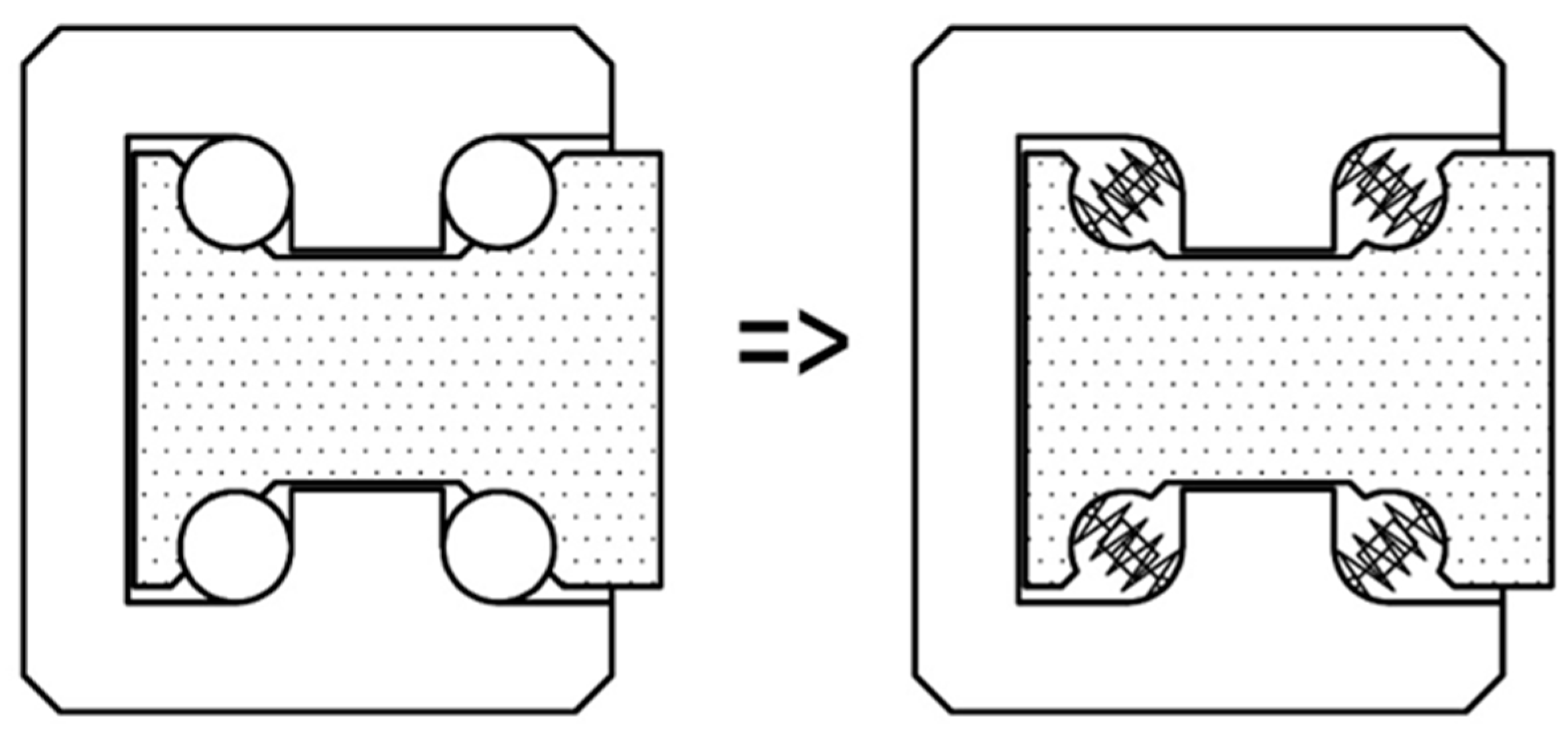
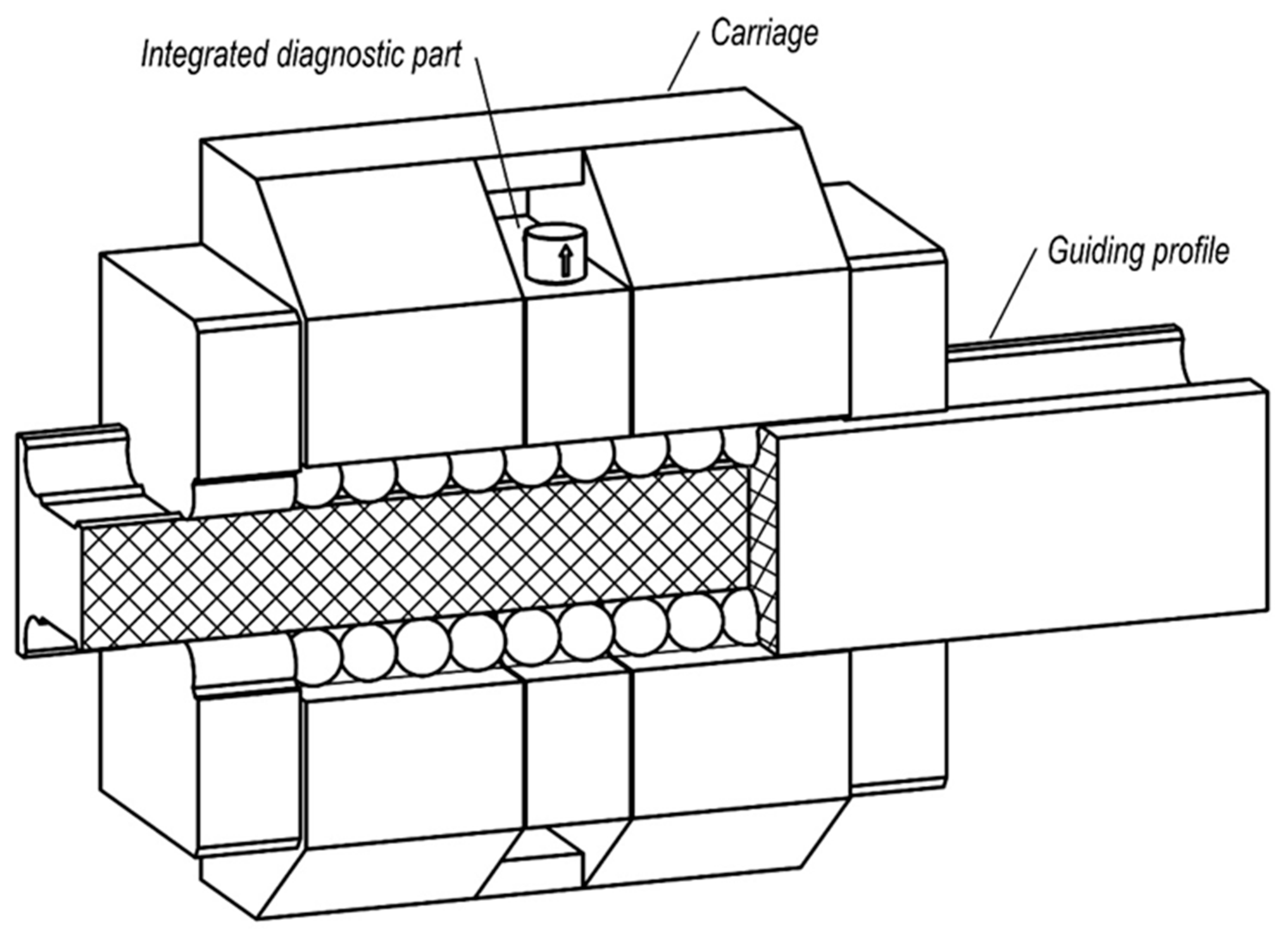
Thus, an original principle of the linear rolling system with an integrated diagnostic system was proposed [24]. A load-free part was designed in the linear system carriage, with shared rolling elements. Through the load-free part, the external dynamical load is eliminated, and the vibrations that are measured on the diagnostic (load-free) part more easily enable the recognition of the damage (Figure 3).

For the verification of the proposed principle, a functional sample was prepared and tested. The testing process, which was divided into two stages, was based on a simulation of the operating conditions and the guiding profile damage. The first stage compared the vibrations that were measured on a loaded and a load-free carriage in three directions. The second stage focused on evaluating the vibrations that were measured on the diagnostic part of the functional sample. Both measurements were processed in the time domain.

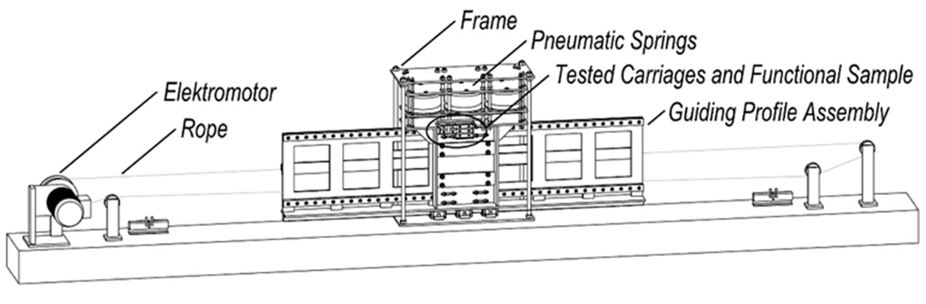
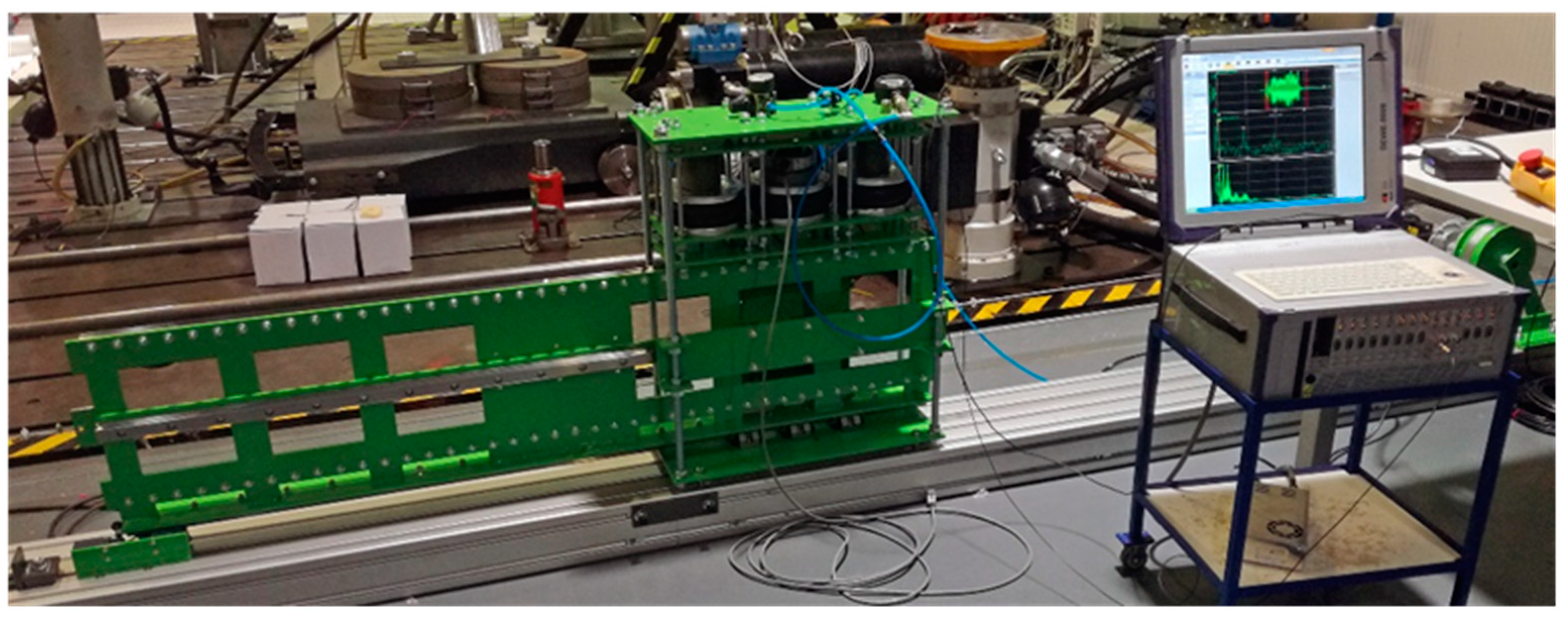
The constructed testing facility enabled the pressure loading of the linear rolling systems by pneumatic springs. A linear motion was ensured by an electromotor through a rope drive (Figure 4 and Figure 5). When testing, the guiding profile assembly moved by velocity (v = 0.42 ms⁻¹), while the tested carriages and the functional sample stood still and were connected by pneumatic springs to the frame. The pressure load that was used for the testing was F = 18.5 kN.

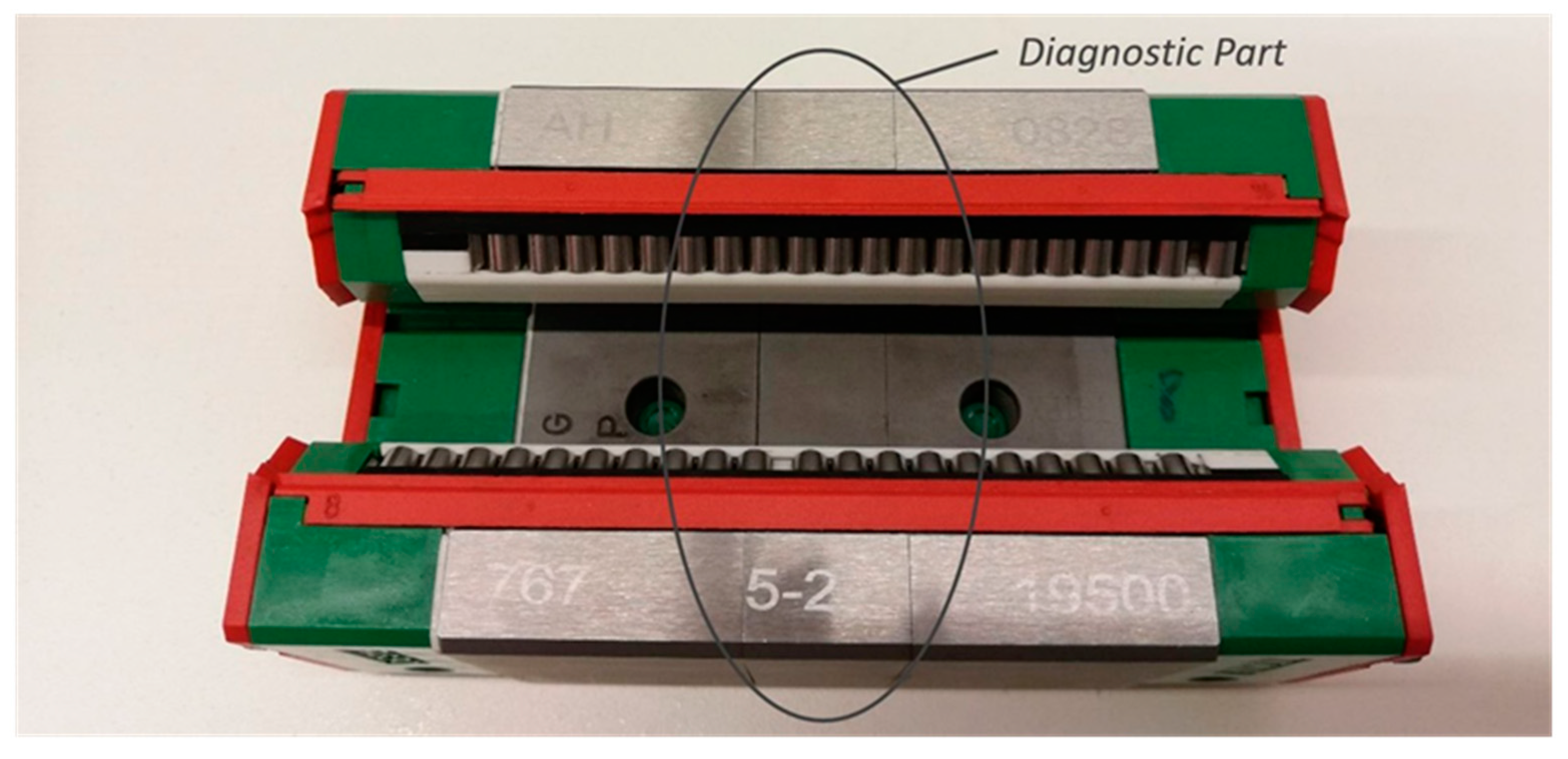
For the functional sample, which was based on the diagnostic part (Figure 6), the Hiwin (Hiwin Technologies Corp., Taichung, Taiwan) linear rolling system was redesigned. Its basic parameters are summarised in

Table 1. Parameters of Hiwin linear rolling system.

Type	Basic Dynamic Capacity	Rolling Elements	Diameter of Rolling Element
Hiwin RGH30CA ZAH	39.1 kN	Rollers	dv = 4 mm

. An iron unit of the carriage was divided into three pieces, with an appropriate clearance fit between them, by combining tinny spacers. The final clearance fit was in the order of hundredths.

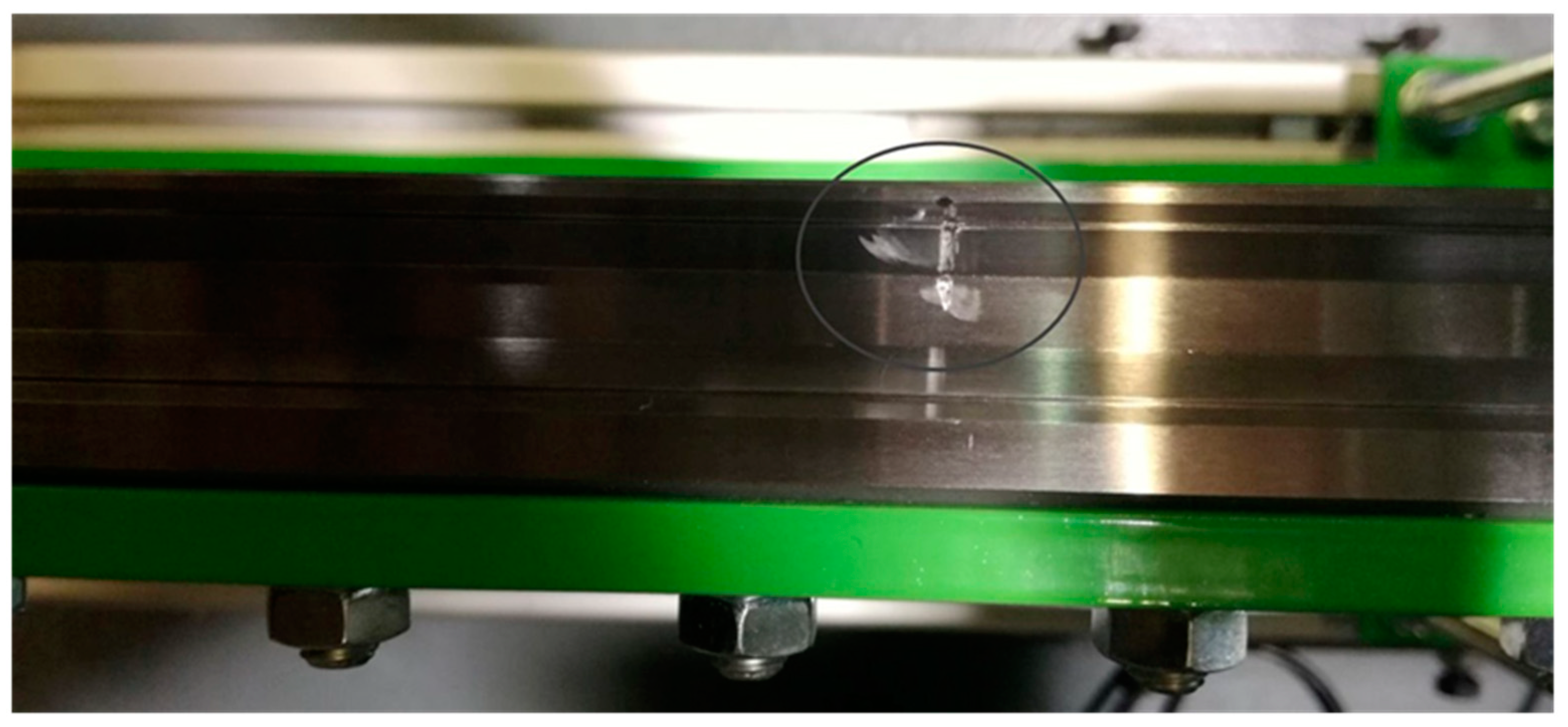
Figure 7 shows the guiding profile damage as a ground groove, with a thickness of 1 mm on the contact surface. The damage represented a fatigue failure that was caused by contact pressure, which occurs by the rolling motion.

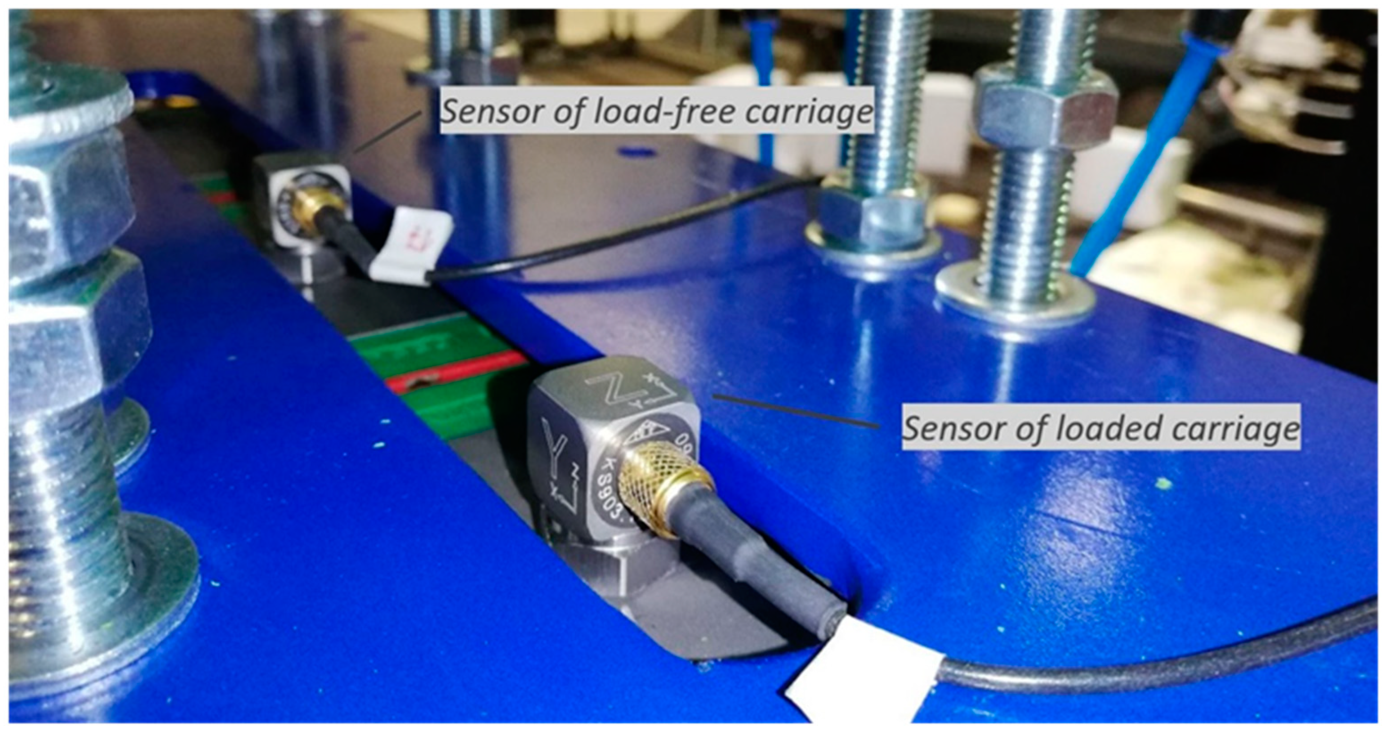
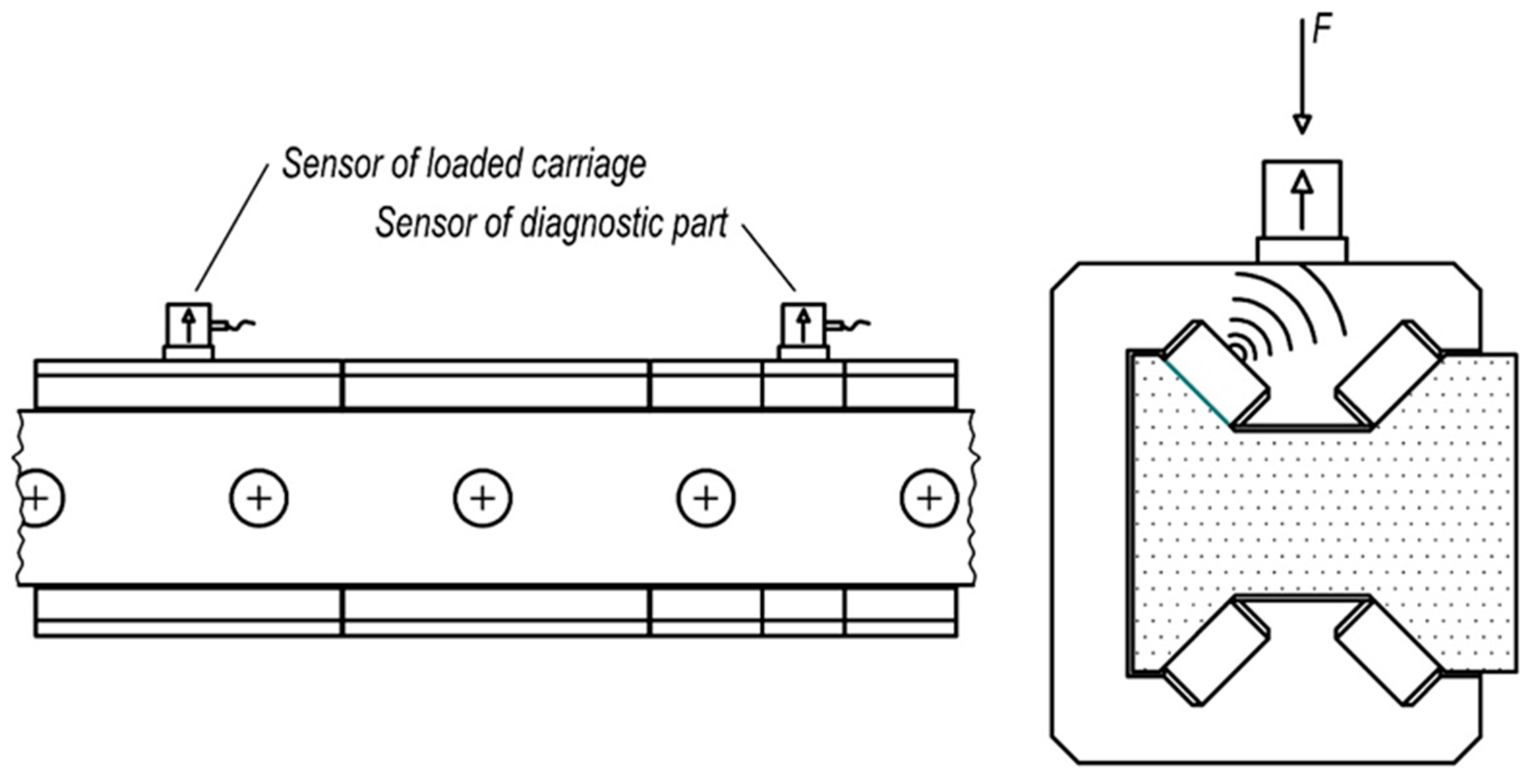
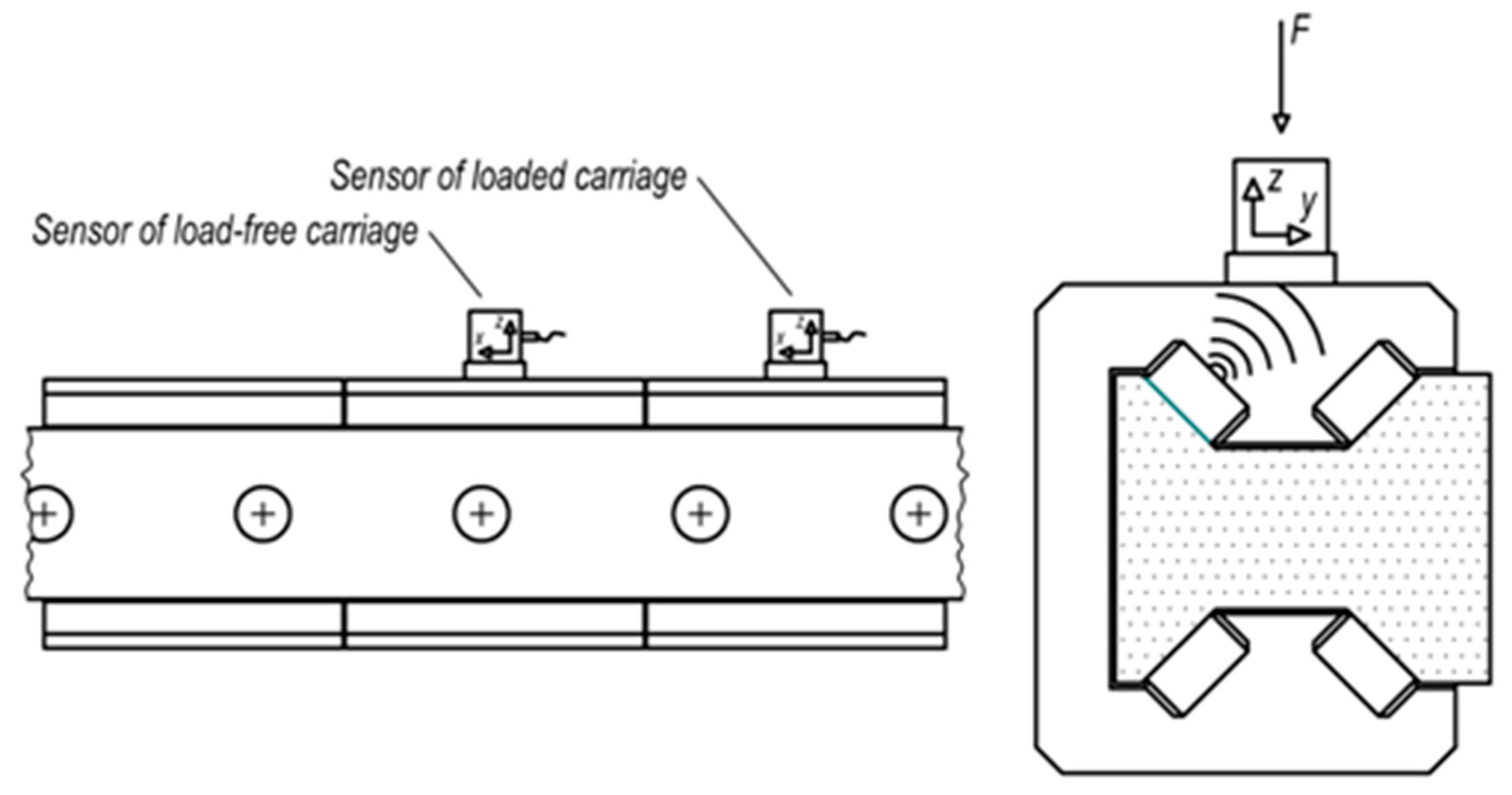
In the first stage of testing, the acceleration sensors were placed according to the scheme in Figure 8. Three-axis sensors were applied for evaluating the vibrations in all three axes. The three-axis sensor of MMF (type: KS903.100) (Manfred Weber Metra Meß- und Frequenztechnik in Radebeul e.K., Radebeul, Germany) featured a range of ±60 G, and a linear frequency range up to 10 kHz. With respect to the linear frequency range of the sensors, a sampling frequency of the measurement was set to 20 kHz. Figure 9 shows the actual sensor positions on the loaded and the load-free carriage.

A similar method to the first stage was employed for testing the functional sample with the integrated diagnostic part. The one-axis acceleration sensors were placed according to the scheme in Figure 10. The one-axis sensor of the MMF producer (type: KS97.100) featured the range of ±60 G and a linear frequency range up to 13 kHz. With consideration to the linear frequency range of the sensors, the sampling frequency was set to 25 kHz. Figure 11 shows the actual sensor positions on the loaded carriage and the diagnostic part of the functional sample.

3. Theory

In the service of linear rolling systems, the contact pressure between the guiding profile and the rolling elements appears because of the external dynamical loads. The cyclic loading and unloading of linear systems causes a relative shift in the contact surfaces that is related to the different radii of their curvatures. Furthermore, the linear motion is characterised by the rolling process of the rolling elements against the guiding profile. The rolling motion leads to the asymmetric deformation of the contact surfaces and to the asymmetric distribution of the contact pressure. This behaviour belongs to the hysteresis of the used material [25,26].

Dynamical changes in the contact pressure as a result of the external load and the rolling motion may generate a fatigue failure, which is called “pitting” or “spalling”. The fatigue failure is represented by a breakout of the contact surface particles, which leaves pits at sufficient lubrication, or spalling at the surface layer at insufficient lubrication [27,28].

The fatigue failure of the rolling elements and the guiding profiles produces a rolling friction increment that decreases the linear system efficiency [29,30,31,32]. The result of the fatigue failure is increases in the temperature, the noise, and the vibrations of linear systems. Vibrations may negatively affect related bodies and even the linear system itself, which contributes to their development.

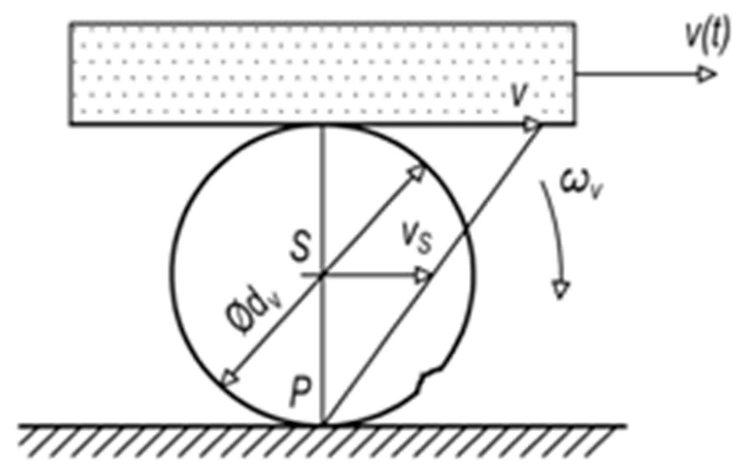
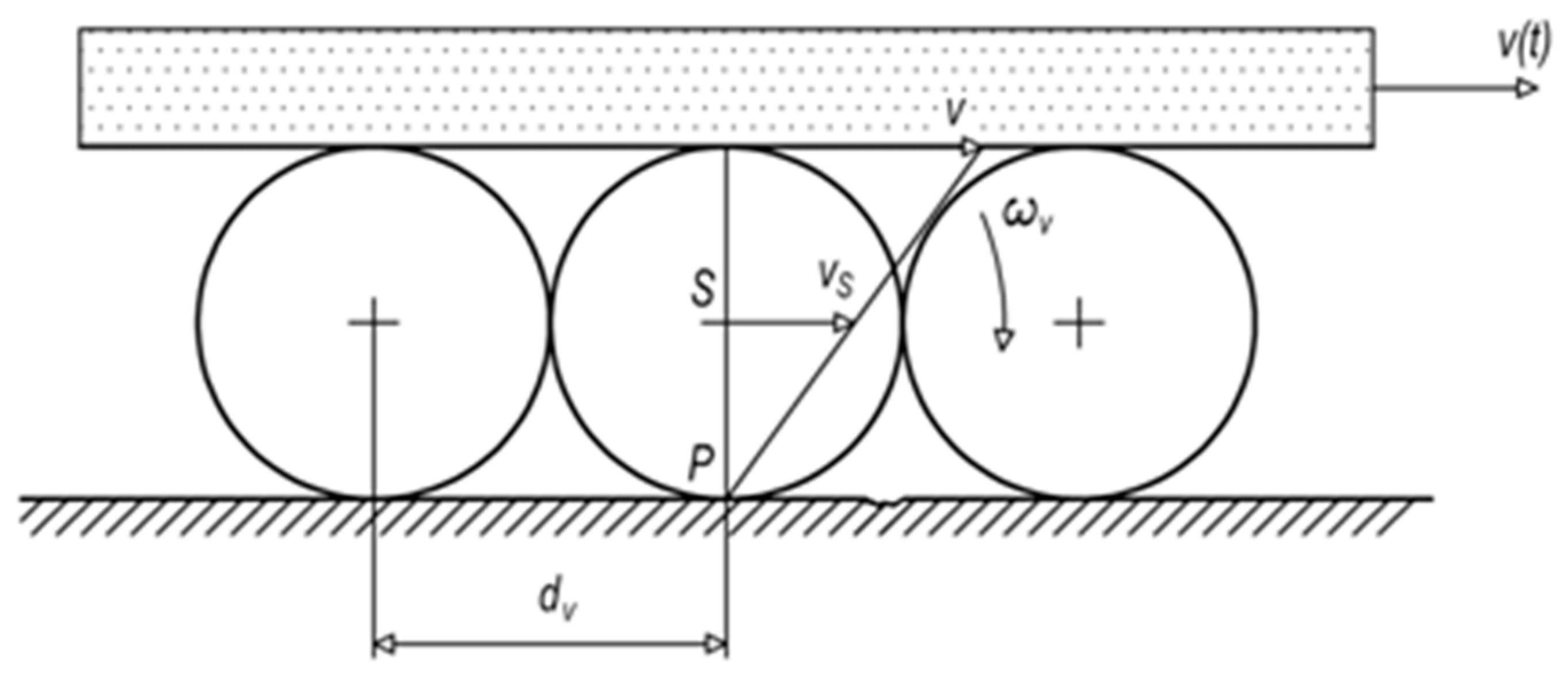
Vibrations present increased amplitudes with regard to the frequency or the time period of the damage. Frequencies may be computed through kinetic analysis for two general cases: for the damage of the rolling element (Figure 12), or for the damage of the guiding profile (Figure 13). According to kinematic schemes, the damage frequencies and time periods depend on the linear motion velocity.

In order to derive the damage frequency of the rolling element, it may be stated that its velocity at the point (P) equals zero, so that:

$$v_P\left(t\right)=v_S\left(t\right)-{\omega }_v\left(t\right)\frac{d_v}{2}=0$$

(1)

where the velocity of the rolling element at the rotation centre (v_s(t)) is related to the velocity of the linear motion (v(t)), by the equation:

$$v\left(t\right)=v_S\left(t\right)+{\omega }_v\left(t\right)\frac{d_v}{2}$$

(2)

Then, the velocity (v_s(t)) may be computed as:

$$v_S\left(t\right)=\frac{v\left(t\right)}{2}$$

(3)

Through the diameter of the rolling element (d_v), the equation for the angular velocity of the rolling element is:

$${\omega }_v\left(t\right)=\frac{2v_S\left(t\right)}{d_v}$$

(4)

The damage time period of the rolling element reflects the vibration excitation by the damage twice in one rotation of the rolling element, at the upper and lower contact surfaces:

$$T_{Dv}\left(t\right)=\frac{2\pi }{2{\omega }_v\left(t\right)}=\frac{\pi d_v}{v\left(t\right)}$$

(5)

Then, the damage frequency is:

$$f_{Dv}\left(t\right)=\frac{1}{T_{Dv}\left(t\right)}=\frac{v\left(t\right)}{\pi d_v}$$

(6)

The damage time period of the guiding profile refers to the time when the rolling element performs a distance of d_v by the velocity (v_S(t)) of the rotation centre:

$$T_{Dp}=\frac{d_v}{v_S\left(t\right)}=\frac{2d_v}{v\left(t\right)}$$

(7)

The damage frequency equals:

$$f_{Dp}\left(t\right)=\frac{1}{T_{Dp}\left(t\right)}=\frac{v\left(t\right)}{2d_v}$$

(8)

For the case of the functional sample, the time periods and the frequencies of damage are summarised in

Table 2. Damage time periods and frequencies of Hiwin linear rolling system.

Rolling Element		Guiding Profile
TDv = 0.03 s	fDv = 33.4 Hz	TDp = 0.019 s	fDp = 0.019 Hz

.

With reference to the proposed principle of the linear system diagnostics on the basis of the integrated diagnostic part, the negative influence of the external loads was observed on the linear system through a simplified mechanical model. In the mechanical model, elastic and damping connections may substitute for the rolling elements [32,33,34,35], and the damage may be represented by kinematical excitation (Figure 14).

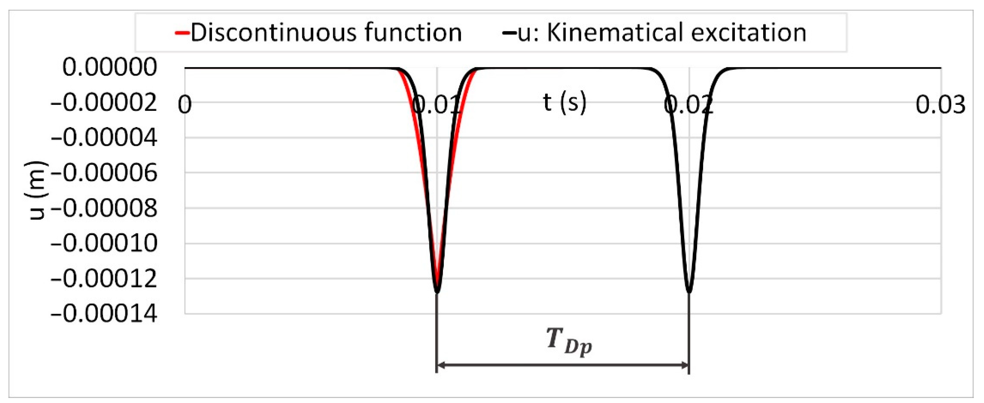
For the kinematical excitation, a hyperbolic tangent function was applied to supplant a discontinuous function that was shaped similar to a rolling element crossing over the damage with a thickness of 1 mm. Figure 15 presents the kinematical excitation with the time period of the guiding profile damage.

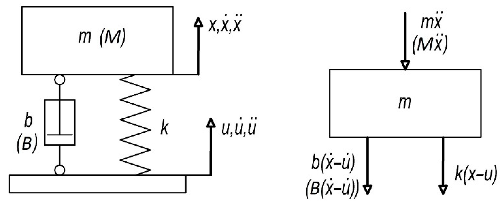
The simplified mechanical model (Figure 16) substitutes elastic connections through reduced stiffness in a radial direction that was provided by the producer’s data. For the damping connections, we used a damping ratio with a value of b_rel = 0.5 [36]. A mass of m represents the mass of the carriage unit, and, in the loaded case, M signifies the mass of the carriage unit and the inertia mass of the hanged bodies.

Table 3. Dynamical parameters of the simplified mechanical model in Figure 16.

Mass of The Carriage Unit	Mass of The Carriage Unit and Hanged Bodies	Stiffness of Rolling Elements	Damping Coefficient of The System without Hanged Bodies (including Sealing Parts and Lubrication)	Damping Coefficient of The System with Hanged Bodies (including Sealing Parts and Lubrication)
m = 0.82 kg	M = 100 kg	k = 1.2 × 106 N·m−1	b$\cong$ 1 × 103 Ns·m−1	B$\cong$ 1 × 104 Ns·m−1

summarises the dynamical parameters of the simplified mechanical model.

The result of the motion differential in Equation (9) is the time relation of the mass acceleration as a system response to the excitation function. For the case without hanged bodies to the carriage, the motion differential equation equals:

$$m\ddot{x}+b\left(\dot{x}-\dot{u}\right)+k\left(x-u\right)=0$$

(9)

With hanged bodies, the motion differential equation equals:

$$M\ddot{x}+B\left(\dot{x}-\dot{u}\right)+k\left(x-u\right)=0$$

(10)

where a damping coefficient (b) equals:

$$b=2b_{rel}\sqrt{mk}$$

(11)

$$B=2b_{rel}\sqrt{Mk}$$

(12)

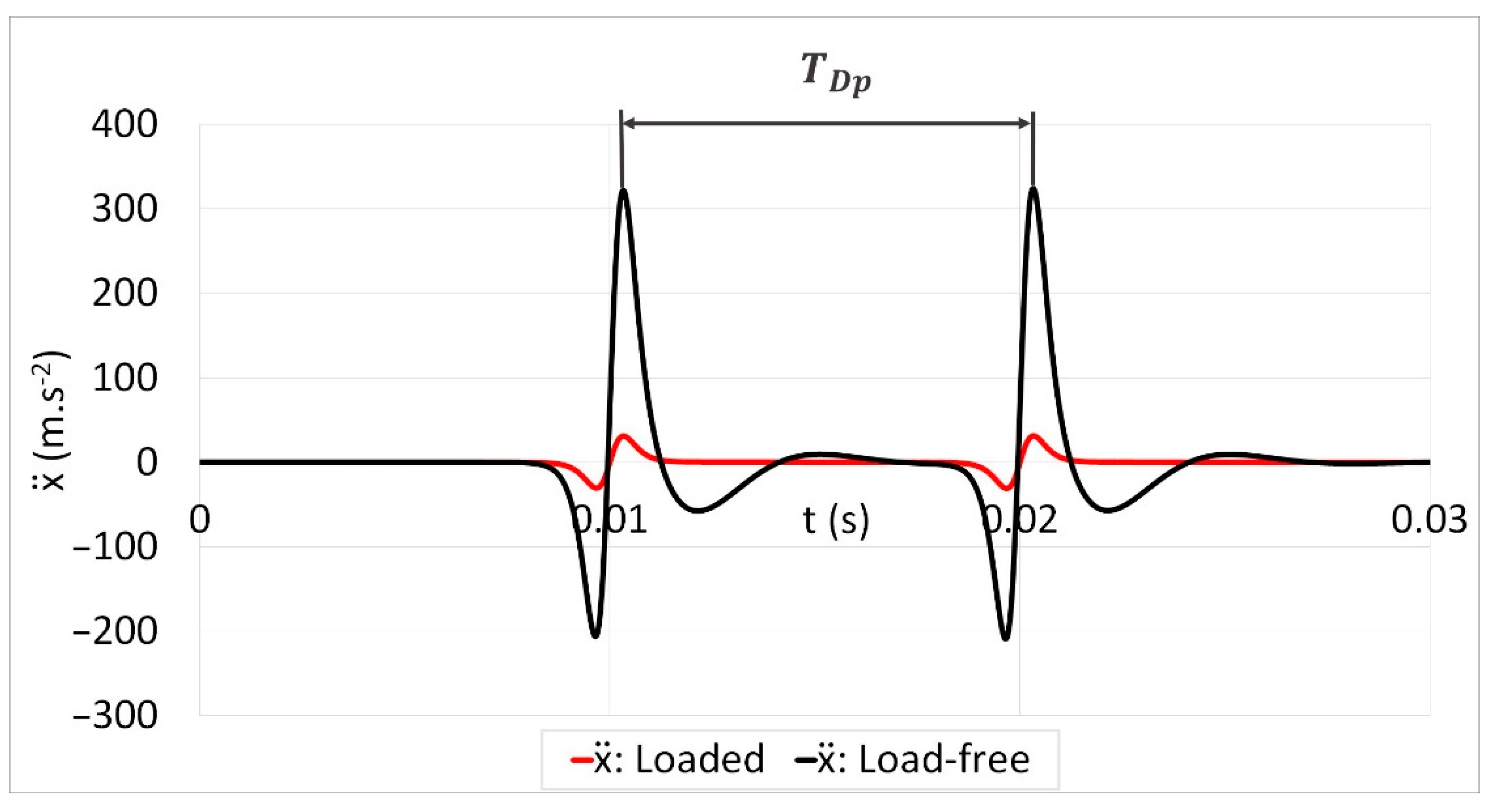
The motion differential in Equations (9) and (10) were processed in MATLAB software, and the results are shown in Figure 17.

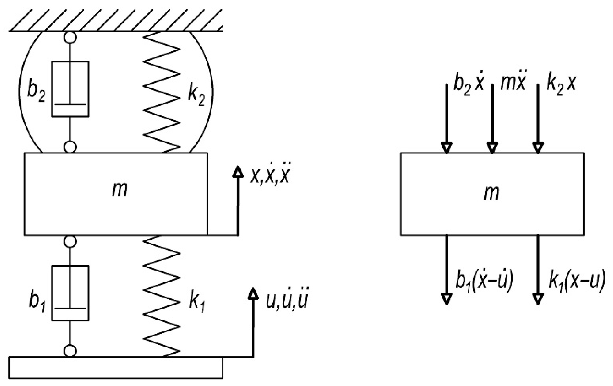
For testing the diagnostic function, the linear rolling system loaded by an external force may be represented through the simplified mechanical model in Figure 18. The external force as the load from the pneumatic springs acts similarly to the mass inertia. By the elastic deformation of the rolling elements, a preload of the linear rolling systems is reached. The preload leads to the system stiffness increase.

In the mechanical model, the stiffness (k₁) and the damping coefficient (b₁) are related to the rolling elements, while k₂ and b₂ belong to the pneumatic springs. The result of the motion differential in Equation (13) is the time relation of the mass acceleration as a system response to the excitation function:

$$m\ddot{x}+b_1\left(\dot{x}-\dot{u}\right)+b_2\dot{x}+k_1\left(x-u\right)+k_{2}x=0$$

(13)

Table 4. Dynamical parameters of the simplified mechanical model in Figure 18.

Mass of The Carriage Unit	Stiffness of Preloaded Rolling Elements	Stiffness of Pneumatic Spring	Damping Coefficient of The System (including Sealing Parts and Lubrication)	Damping Coefficient of Pneumatic Springs
m = 0.82 kg	k1 = 3.6 × 107 N·m−1	k2 = 8 × 103 N·m−1	b1$\cong$ 5 × 103 Ns·m−1	b2$\cong$ 80 Ns·m−1

summarises the dynamical parameters of the simplified mechanical model loaded by the external force.

The motion differential in Equation (13) was processed in MATLAB software, and the results are shown in Figure 19.

In both cases, loading the linear rolling system by the external load in the form of mass inertia or external force showed a significant reduction in the acceleration ($\ddot{x}$), which was excited by the damage.

4. Results and Discussion

The diagnostic function of the proposed diagnostic principle was verified via the testing facility under the abovementioned conditions. On the contact surface of the guiding profile, the groove was ground for the damage simulation. Then, the vibrations of the loaded and the load-free carriage, and the diagnostic part of the functional sample, were measured and analysed in the time domain.

In the first stage of testing, the influence of the external load and the measurement direction was decided for vibrations that were excited by the simulated damage. The load-free carriage was placed between two that were tightly connected to the testing facility, and, finally, the mentioned effects were evaluated.

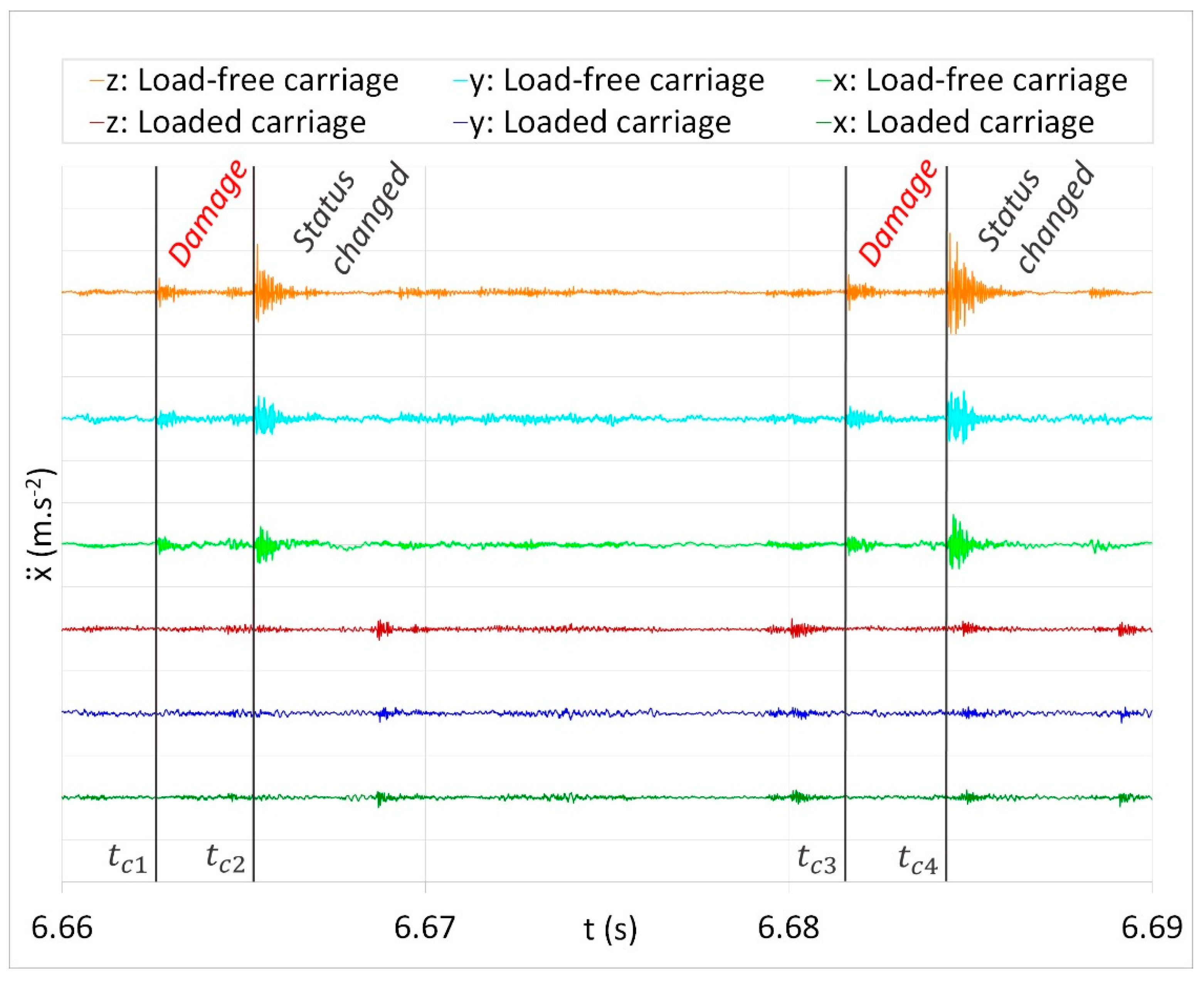
The time graph in Figure 20 shows the measured acceleration of the vibrations in the time domain at the loaded carriage crossing over the simulated damage. Major amplitudes of the measured acceleration may be recognised at a time period of T_cBA with the parameters summarised in

Table 5. Time period and its parameters according to Figure 20.

Parameters		Time Period
tcA = 7.24420 s	tcB = 7.26425 s	TcBA = 0.02 s

.

The time period (T_cBA) equals:

$$T_{cBA}=t_{cB}-t_{cA}$$

(14)

These amplitudes might be observed through the entire time of the carriage motion. Thus, it may be noted that the major amplitudes belong to the changed status of the rolling element from nonloaded to loaded. The amplitudes of acceleration that could be related to the simulated damage are hidden in the vibration noise.

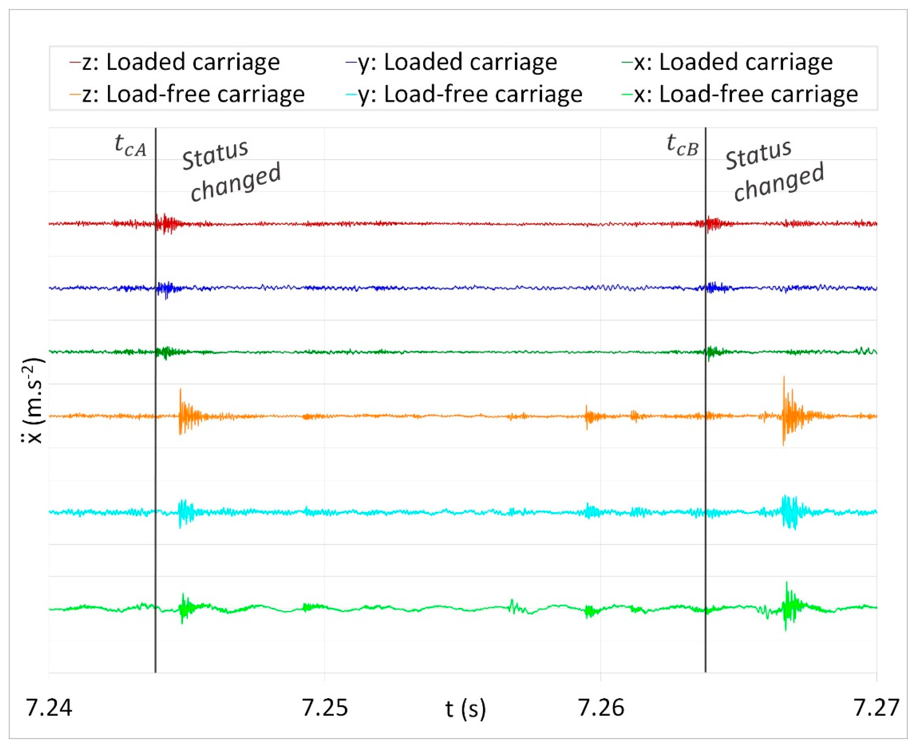
The time graph in Figure 21 illustrates the measured acceleration of the vibrations in the time domain at the load-free carriage crossing over the simulated damage. The time parameters of the major (T_c42) and minor (T_c31) acceleration amplitudes may be detected with the parameters that are specified in

Table 6. Time periods and their parameters according to Figure 21.

Time Parameters				Time Periods
tc1 = 6.66275 s	tc2 = 6.66555 s	tc3 = 6.68135 s	tc4 = 6.68455 s	Tc21 = 0.0023 s	Tc43 = 0.0027 s

.

As can be seen in the time graph, the major amplitudes of the acceleration with the time period of T_c42 belong to the changed status of the rolling element from nonloaded to loaded. In the measured vibrations, minor amplitudes of acceleration (T_c31) may be observed. These amplitudes are related to the vibrations that were excited by the simulated damage:

$$T_{c42}=t_{c4}-t_{c2}$$

(15)

$$T_{c31}=t_{c3}-t_{c1}$$

(16)

The time period of the major and minor amplitudes is approximately equal to the damage time period of the guiding profile: T_c42 ≅ T_c31 ≅ T_Dp. Through the time phases, ΔT_c21 and ΔT_c43, between the major and minor amplitudes, the damage position against the current position of the rolling elements can be determined:

$$\Delta T_{c21}=t_{c2}-t_{c1}$$

(17)

$$\Delta T_{c43}=t_{c4}-t_{c3}$$

(18)

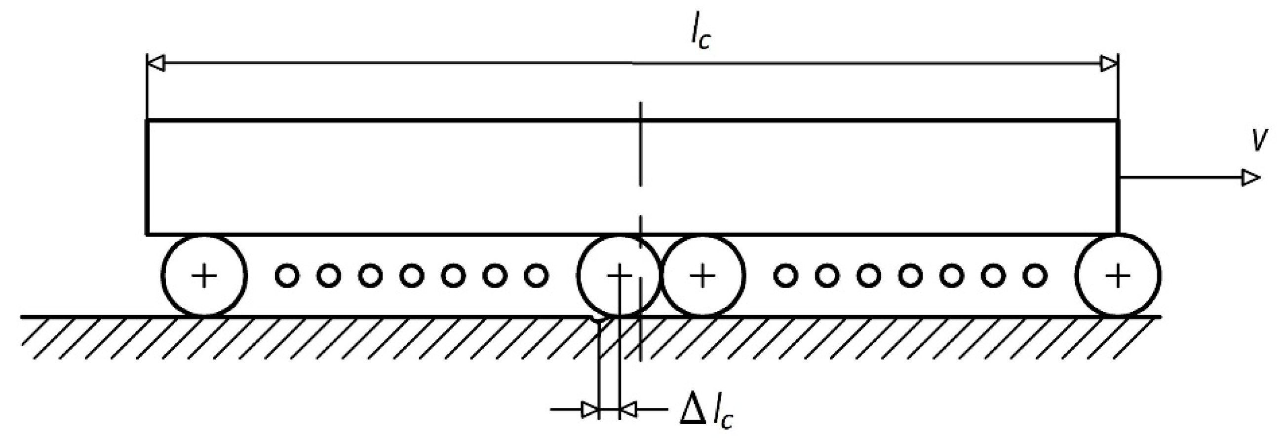
The distance (Δl_c) of the simulated damage against the rolling elements is roughly equal to:

$$\Delta l_c\cong \frac{1}{2}\Delta T_{c21}v\cong \frac{1}{2}\Delta T_{c43}v$$

(19)

Through the length of the iron unit (l_c), a number of rolling elements (n_c) in contact with one raceway of the guiding profile may be calculated:

$$n_c=\frac{l_c}{d_v}$$

(20)

The results of Equations (17)–(20), which are summarised in

Table 7. Results of Equations (17)–(20).

Time Phases		Distance of Simulated Damage against Rolling Elements	Length of The Iron Unit	Number of Rolling Elements in Contact with One Raceway of Guiding Profile
ΔTc21 = 0.0023 s	ΔTc43 = 0.0027 s	Δlc $\cong$ 0.5 mm	lc = 71 mm	nc = 17.75

, indicate 17 or 18 rolling elements in contact with the raceway at each time (Figure 22).

According to the analysis of the measured acceleration, it may be stated that the external load of linear systems is directly related to the early detection of possible failure. In the loaded carriage, the measured amplitudes of acceleration are significantly lower than in the load-free carriage; and the amplitudes related to the vibrations that were excited by the simulated damage are hidden in the vibration noise.

The acceleration of vibrations was measured and evaluated in three coordinate axes: x, y, and z. In the case of the loaded carriage, the amplitudes of acceleration in all the axes reached similar values. Therefore, vibrations can be measured in any direction, and their amplitudes are independent of the loading force direction. In the load-free carriage, a difference may be observed between the amplitudes measured in the z-axis (radial) direction and the amplitudes measured in the other two axes directions. This attribute might be related to the gravitational acceleration that acts in the same direction. Thus, the one-axis sensor was placed in the appropriate direction for the subsequent testing.

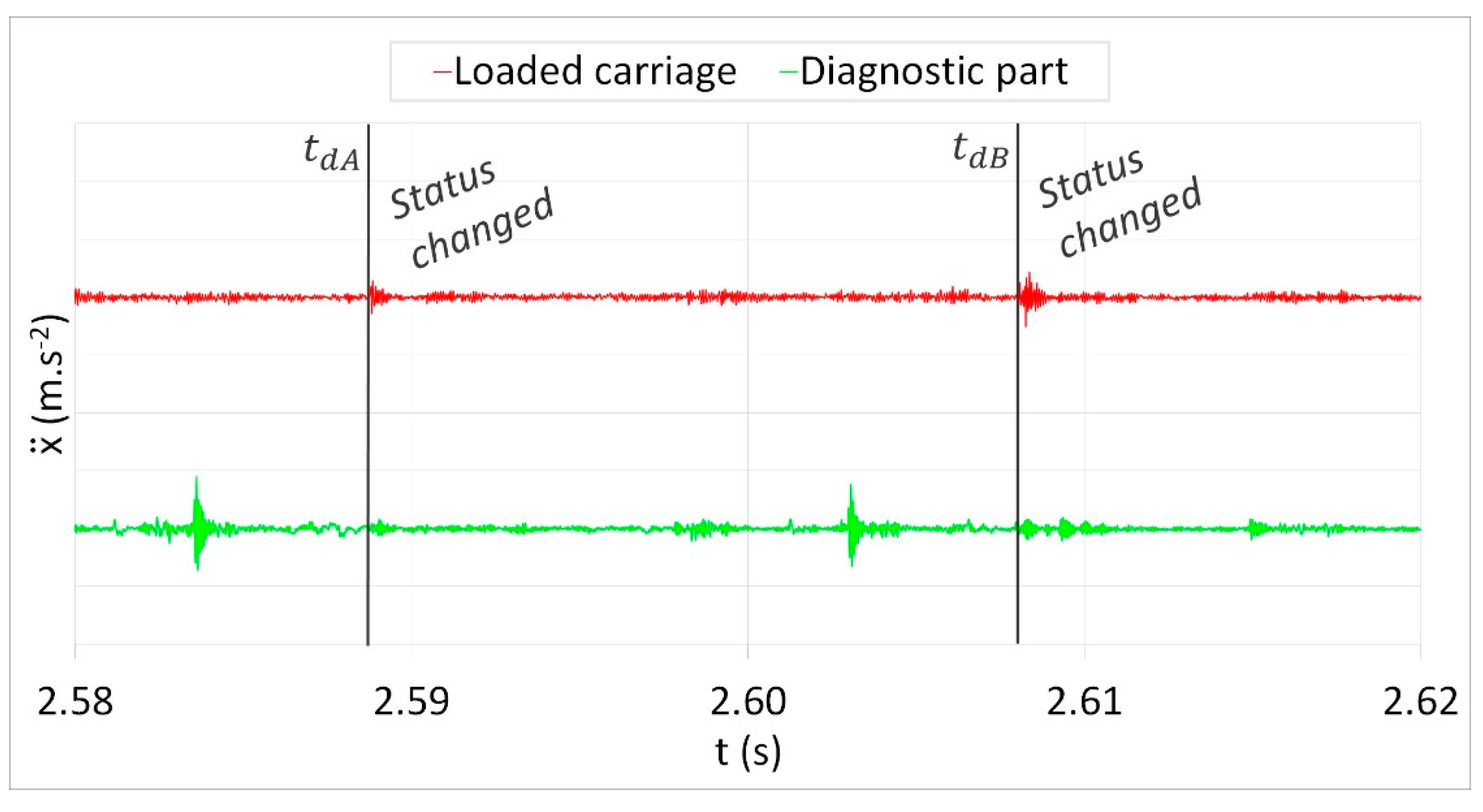
In the second stage, the functional sample with the integrated diagnostic part was analysed. The time graph in Figure 23 shows the measured acceleration of the vibrations in the time domain at the loaded carriage crossing over the simulated damage. Major amplitudes of measured acceleration may be recognised at a time period of T_dBA with the parameters that are summarised in

Table 8. Time period and its parameters according to Figure 23.

Time Parameters		Time Period
tdA = 2.58904 s	tdB = 2.60804 s	TdBA = 0.019 s

:

$$T_{dBA}=t_{dB}-t_{dA}$$

(21)

It might be noted that these amplitudes belong to the changed status of the rolling element from nonloaded to loaded. In contrast, the amplitudes of acceleration related to the simulated damage are hidden in the vibration noise.

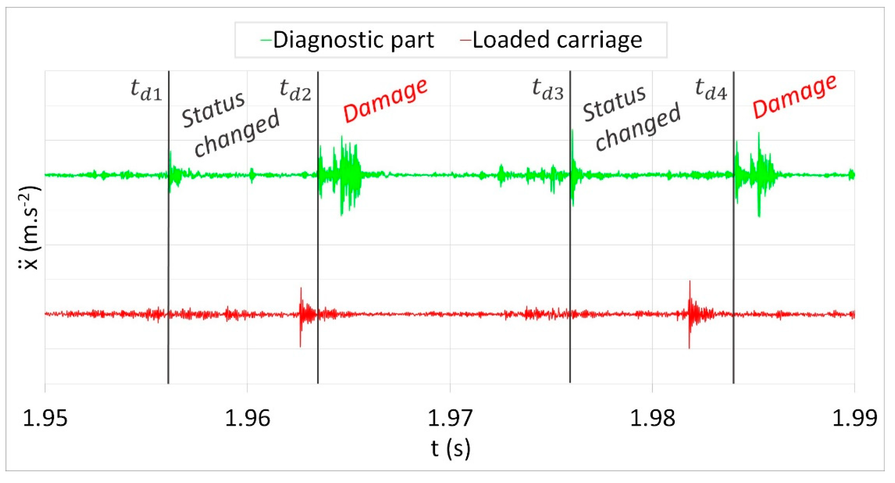
The time graph in Figure 24 illustrates the measured acceleration of the vibrations in the time domain at the diagnostic part crossing over the simulated damage. The time parameters of the major (T_d42) and minor (T_d31) acceleration amplitudes may be detected with the parameters that are specified in

Table 9. Time periods and their parameters according to Figure 24.

Parameters				Time Periods
td1 = 1.95636 s	td2 = 1.96376 s	td3 = 1.97620 s	td4 = 1.98432 s	Td21 = 0.0206 s	Td43 = 0.0198 s

.

The time periods, T_d42 and T_d31, are equal to:

$$T_{d42}=t_{d4}-t_{d2}$$

(22)

$$T_{d31}=t_{d3}-t_{d1}$$

(23)

As can be seen in the time graph, the major amplitudes of acceleration with the time period of T_d42 belong to the vibrations that were excited by the simulated damage. In the measured vibrations, minor amplitudes of acceleration (T_d31) may be observed. These amplitudes are related to the changed status of the rolling element by crossing over from the diagnostic (load-free) to the loaded part of the functional sample.

The time period of the major and minor amplitudes are approximately equal to the damage time period of the guiding profile: T_d42 ≅ T_d31 ≅ T_Dp. Through the time phases, ΔT_d21 and ΔT_d43, between the major and minor amplitudes, the damage position against the current position of the rolling elements can be determined:

$$\Delta T_{d21}=t_{d2}-t_{d1}$$

(24)

$$\Delta T_{d43}=t_{d4}-t_{d3}$$

(25)

The distance (Δl_d) of the simulated damage against the rolling elements is roughly equal to:

$$\Delta l_d\cong \frac{1}{2}\Delta T_{d21}v\cong \frac{1}{2}\Delta T_{d43}v$$

(26)

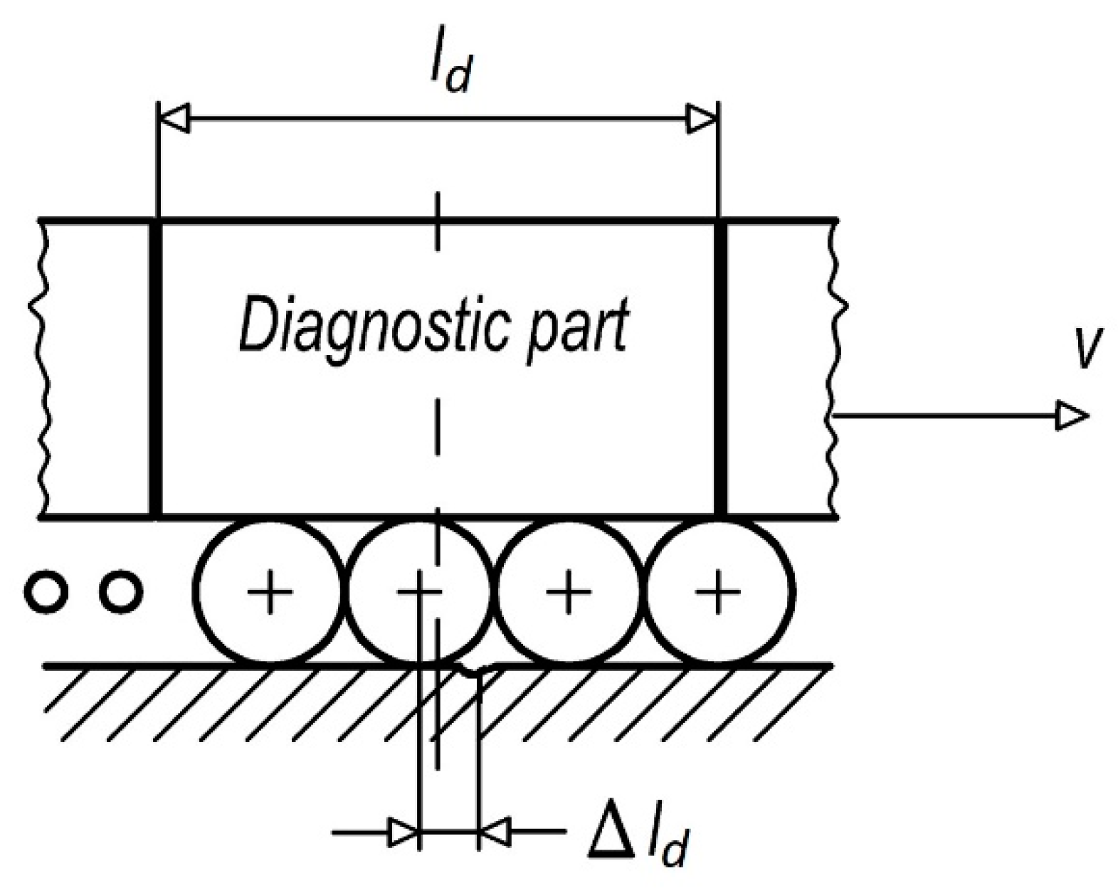
Through the length of the diagnostic part (l_d), a number of rolling elements (n_d) in contact with one raceway of the guiding profile may be calculated:

$$n_d=\frac{l_d}{d_v}$$

(27)

The results of Equations (24)–(27), which are summarised in

Table 10. Results of Equations (24)–(27).

Time Phases		Distance of Simulated Damage against Rolling Elements	Length of The Iron Unit	Number of Rolling Elements in Contact with One Raceway of Guiding Profile
ΔTd21 = 0.0074 s	ΔTd43 = 0.0081 s	Δld ≅ 1.6 mm	ld = 15 mm	nd = 3.75

, indicate 3 or 4 rolling elements in contact with the raceway at each time (Figure 25).

Compared with the load-free carriage, the number of rolling elements in contact with the guiding profile is reduced. With consideration to the preload of the linear systems, by crossing one specific rolling element over the damage, the remaining rolling elements might absorb the excited vibrations. Significant changes may be noticed in the time character of the measured accelerations. By reducing the number of the rolling elements in contact with the guiding profile, significant acceleration amplitudes belonging to the vibrations that were excited by the simulated damage were reached.

5. Conclusions

The diagnostics of linear rolling systems is currently based on measuring vibrations and evaluating the RMS value in the context of the threshold value. In transportation practice, we registered several cases of failure without exceeding the threshold value of the vibrations. Therefore, the original principle of diagnostics was proposed on the basis of minimising the external load through the load-free (diagnostic) part that is integrated into the linear system carriage. Through testing, it was proven that the innovative diagnostic principle enables the early detection of failures, even if the linear rolling system is operated under great external loads.

In the first stage, the vibrations that were measured on the loaded and load-free carriage were compared in the time domain. The main conclusions of the first-stage testing are:

• The external load of linear systems negatively affects the early detection of possible failure;
• In the loaded carriage, the vibrations that were excited by the simulated damage were hidden in the measured vibrations;
• In the load-free carriage, minor amplitudes of vibrations were observed in the measured vibrations.

In the second stage, the functional sample with the integrated diagnostic part was designed and tested. The vibrations that were measured on the loaded carriage and the load-free diagnostic part were compared in the time domain. The main conclusions of the second-stage testing are:

• In the loaded carriage, the vibrations that were excited by the simulated damage were hidden in the measured vibrations;
• In the diagnostic part, the major amplitudes related to the simulated damage were registered;
• The major amplitudes at the diagnostic part were reached by reducing the number of rolling elements in contact with the raceway, and by further reducing the external load as the mass inertia of the diagnostic part.

It should also be noted that the vibrations that were excited by the simulated damage appeared once, at a particular time. In the load-free carriage, theoretically, eighteen acceleration amplitudes related to the damage might be noticed in the measured data, and in the diagnostic part, only four. In general, the vibrations that are associated with possible failure dispose of their nonperiodical character and cannot be easily processed in the frequency domain.

The initial results of the original diagnostic principle of linear rolling systems are introduced in the paper. Further research is needed in order to reach sufficient reliability of the diagnostic function and to obtain an adequate life of the redesigned carriage. The research should be focused on a methodology of early failure identification, with respect to the wear progression, the level of lubrication, and the variable operating conditions, both kinematic and dynamical. An optimised design of the functional sample should be tested for its life and load capacity. Further research should also deal with the automatic processing of the measured vibrations, which should aim at the implementation of innovative diagnostics into transportation practice.