Abstract
We investigated liquid freshwater content (FWC) in the upper 100 m layer of the Arctic Ocean using oceanographic observations covering the period from 1990 through 2018. Our analysis revealed two opposite tendencies in freshwater balance—the freshening in the Canada Basin at the mean rate of 2.04 ± 0.64 m/decade and the salinization of the eastern Eurasian Basin (EB) at the rate of 0.96 ± 0.86 m/decade. In line with this, we found that the Arctic Ocean gained an additional 19,000 ± 1000 km3 of freshwater over the 1990–2018 period. FWC changes in the EB since 1990 demonstrate an intermittent pattern with the most rapid decrease (from ~5.5 to 3.8 m) having occurred between 2000 and 2005. The 1990–2018 FWC changes in the upper ocean were concurrent with prominent changes of the thermohaline properties of the intermediate Atlantic Water (AW)—the main source of salt and heat for the Arctic Basin. In the eastern EB, we found a 50 m rise of the upper AW boundary accompanied by a ~0.5 °C increase in the AW core temperature. The close relationship (R > 0.7 ± 0.2) between available potential energy in the layer above the AW and FWC in the eastern EB suggests a positive feedback mechanism that links the amount of freshwater with the intensity of vertical heat and salt exchange in the halocline and upper AW layers. Together with other mechanisms of Atlantification, this feedback creates a complex picture of interactions behind the observed changes in the hydrological and ice regimes of the Eurasian sector of the Arctic Ocean.
1. Introduction
The Arctic Ocean is one of the most significant freshwater reservoirs accumulating about 11% of the global continental runoff [1,2,3]. Along with the continental runoff, the Arctic Ocean’s freshwater/salt balance is strongly influenced by inflows from the adjacent sectors of the Pacific and Atlantic Oceans [4,5,6,7,8]. Other contributing factors are the influence of atmospheric circulation, moisture transport from the mid-latitudes, sea ice state, and upper ocean currents [6,9,10,11,12,13]. In the Arctic Ocean, the redistribution of freshwater affects ocean stratification, producing numerous feedback mechanisms (positive and negative) among physical and biological components in the climate system [6,14,15]. One example illustrating the impact of freshwater on ocean stratification involves the increase in the melting of sea ice at the ocean surface that results in the suppressed mixing and reducing of ocean heat fluxes from the intermediate ocean layers to the upper ocean and the bottom of sea ice [16,17]. In contrast, the loss of surface fresh layer provides favorable conditions for deeper winter ventilation and is associated with larger vertical heat fluxes (the “halocline catastrophe”), which may have irreversible consequences for the hydrological regime of some regions of the Arctic Ocean [15,17,18].
In conditions of changing arctic climate, the relations between primary freshwater sources and processes underlying the dynamics of freshwater variability in the Arctic Ocean are not fully understood yet (see [6] for discussion). For instance, following the estimates by Serreze et al. [19], the annual inflow of freshwater into the Arctic Ocean is dominated by river runoff (42%), with the second and third contributors being the inflow from the Pacific Ocean through Bering Strait (32%) and atmospheric precipitations (26%). However, earlier estimates (e.g., [17]) suggested different contributions of 56% for the river runoff, and 28 and 15% contributions associated with the inflow through Bering Strait and precipitation, respectively. A discrepancy between published estimates of freshwater balance in the Arctic Ocean (e.g., [10,12,20,21] and others) as well as uncertainty of the mechanisms and regional consequences of its change make studies of freshwater changes based on the analysis of in situ data essential to understanding the trajectories of polar climate change.
Here, we present reconstructions of liquid freshwater content in the upper ocean layer of the Arctic Ocean in the 1990s, 2000s, and 2010s. A particular focus of this study was on the Eurasian sector of the Arctic Ocean (Figure 1), where we found direct impact of freshwater changes on density stratification. This article is organized as follows. After the introduction, we provide an overview of observational data utilized in our study alongside a detailed description of the methods implemented (Section 2). In Section 3, we describe large-scale patterns of freshwater content (FWC) and examine their changes over the last three decades. Section 4 includes a discussion of long-term freshwater changes in the context of Atlantic Water (AW) and stratification changes in different parts of the Arctic Ocean. The paper concludes with the final section in which we summarize the most significant findings.
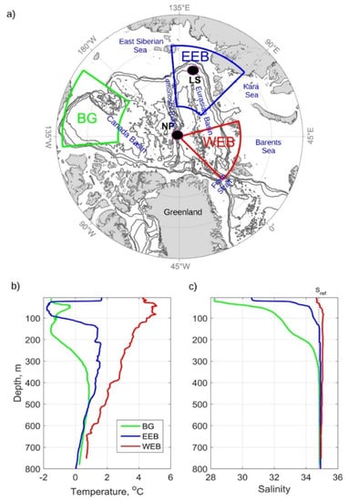
Figure 1.
(a) Map of the Arctic Ocean showing geographic locations of major basins used in our study. WEB, EEB, and BG indicate the western Eurasian Basin, the eastern Eurasian Basin, and the Beaufort Gyre, respectively. Black circles show the positions of the Laptev Sea and North Pole regions. Grey contours show bottom depth isobaths. (b,c) Typical summer (September) temperature and salinity profiles collected in the BG (80° N, 146° W), EEB (78.5° N, 126° E), and WEB (81.5° N, 26° E) in the 2010s. Dashed line in (c) indicates the reference salinity (Sref) of 34.8 used in our calculations.
2. Data and Methods
2.1. Oceanographic Data
In the present study, we used temperature (T) and salinity (S) observations collected in the Arctic Ocean starting from the 1990s until recent oceanographic surveys in 2018. Most CTD (conductivity-temperature-depth) profiles included in the dataset were acquired with modern CTD instruments with a high (~1 m) vertical resolution. The sources of these data include the world’s largest centers for polar oceanographic data such as the National Centers for Environmental Information (NCEI) and the International Council for the Exploration of the Sea (ICES). We also included data from numerous data portals developed by observational programs carried out in the last two decades (e.g., the Distributed Biological Observatory, Beaufort Gyre Observational System, Nansen and Amundsen Basins Observational System, and others). Before use, the data were screened for duplicates to avoid possible biases in the calculated statistics.
The ship-based observations were complemented by temperature and salinity profiles from autonomous Ice-Tethered Profilers (ITPs; https://www.whoi.edu/page.do?pid=20756, (accessed on 16 April 2020)). Their inclusion enables an assessment of the winter hydrography in the central Arctic Ocean, which is poorly covered with in situ observations due to severe ice conditions. All temperature and salinity profiles in the final dataset were additionally re-evaluated for the reliable ranges of variability (0 < S < 36; −2 < T < 20 °C) and presence of unphysical outliers. The previous version of this dataset was used to analyze regional climatic changes in the Arctic Ocean and dynamics of the circumpolar boundary current and mesoscale eddies (e.g., [22,23,24,25,26]). For this study, the dataset was significantly updated with newly available observations so that the final CTD array contained more than 110 thousand oceanographic profiles for the 1990–2018 period (see Figure 2 for decadal maps with data coverage). We limited our analysis to the last three decades due to sparse data coverage in the central and eastern Arctic Basins in previous decades; an insufficient amount of data prevents compiling reliable FWC time series without significant gaps.
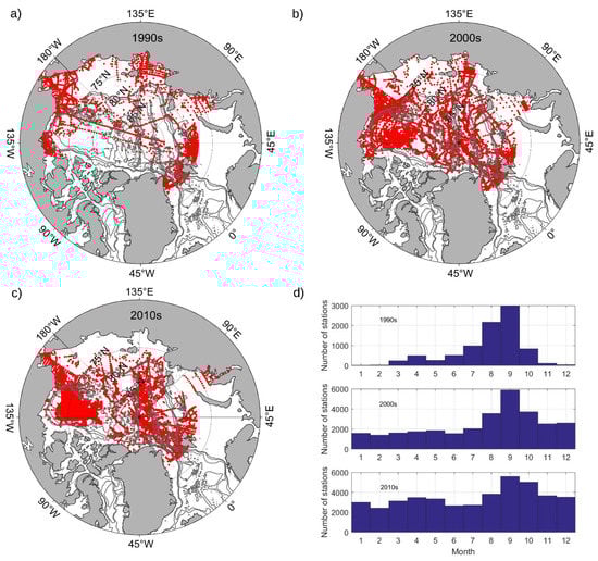
Figure 2.
(a–c) Maps showing decadal distributions of oceanographic stations in the Arctic Ocean in the 1990s–2010s. (d) Monthly distributions of the number of stations in the utilized dataset.
Since the 1990s, most oceanographic observations have been made using precise CTD instruments that measure temperature and salinity with accuracies of about 0.001 °C and 0.003, respectively. However, a significant portion (~13 %) of observations in our dataset were obtained using Nansen bottles and conducted with mercury thermometers with higher measurement errors. Their accuracies are estimated as 0.01 °C for temperature and 0.02 for titrated salinity.
2.2. Freshwater Content
Following Aagaard & Carmack [17], liquid freshwater content was calculated by integrating the departure of measured salinity S(z) from the reference salinity Sref; the latter in our study was chosen as Sref = 34.8:
where zup and zdown are the depths of upper and lower boundaries of the layer and z is the downward vertical coordinate.
Almost all oceanographic profiles included in the final dataset had the shallowest measurements well below the ocean surface (on average, at ~13 m depth), affecting estimates of freshwater content in the upper layer. We approached this problem by extrapolating salinity measurements from the uppermost observational level to the ocean surface so that the salinity distribution in that layer becomes vertically uniform [8,27]. However, if there were no salinity observations made within the upper 15 m, those profiles were eliminated from FWC calculations for the upper layer.
2.3. Density Stratification and Available Potential Energy
Density stratification in the Arctic Ocean plays a crucial role in regulating the vertical exchange of salt and heat between the upper and intermediate layers (e.g., [28,29,30]). In our study, ocean stratification was quantified in two ways. A continuous stratification was evaluated using Brunt–Väisälä buoyancy frequency (N),
where g is the acceleration due to gravity, ρ is the potential density of sea water, and ρ0 is the mean water density of 1027 kg m−3.
In addition to the Brunt–Väisälä frequency, we estimated available potential energy (APE) as an informative integral indicator of stratification in the Arctic Ocean (e.g., [31,32,33]). APE is based on vertical distribution of the potential density within the specified ocean layer and was calculated for each CTD profile as:
where ρref is the potential density at zdown depth.
2.4. Reconstruction of Temporal Changes
The sufficient amount of hydrographic data included in the final dataset enabled us to reconstruct T, S, FWC, N2, and APE in the upper ocean (0–50 m), halocline (50–150 m), and intermediate (150–1000 m) layers in several regions of the Arctic Ocean: the North Pole area—89.5–90° N; Laptev Sea slope—77–79° N, 125–127° E; etc. (Figure 1a) from 1990 through 2018. To illustrate temporal variability of these parameters, we produced time–depth diagrams and regional time series. Time vs. depth diagrams were constructed by implementing a vertical linear interpolation for all CTD profiles in a specific region (within the range of geographical coordinates) to obtain a uniform 1 m vertical resolution. Then, the uniform T, S profiles were interpolated linearly in time, combining into a 2D matrix with a daily temporal resolution. Since our study focused on annual to decadal temporal scales, we additionally performed low-pass filtering of these data using a 6 month running average to reduce the influence of synoptic and monthly variability. This approach was implemented to reconstruct temperature and salinity distributions that were used further to calculate other parameters. For instance, the reconstructed salinity matrix was used to generate FWC time series in a way described in Section 2.2.
Basin-wide regional time series in the Arctic Ocean, i.e., in the eastern Eurasian Basin—EEB (75–85° N; 90–140° E), western Eurasian Basin—WEB (80–89.5° N; 0–60° E), and Beaufort Gyre—BG (71–80° N; 70–160° W) (Figure 1a) were constructed differently. Monthly mean FWC between 1990 and 2018 were calculated on a set of cells covering the Arctic Ocean domain with sizes of 2 and 5 degrees by latitude and longitude, respectively. In each cell, we averaged individual FWC estimates for the specific month and year. Annual values were constructed from monthly FWC estimates. The uneven distribution of oceanographic observations inside the EEB, WEB, and BG was taken into account by splitting an averaging area into four sectors by latitudes and longitudes. Within each sector, the averaging was carried out independently. After that, the averaged sectoral values were averaged again, taking into account their weights proportional to the area of each sub-sector. For the last two decades (the 2000s and 2010s), such an approach allowed us to add more weight to ship-based observations by comparison to densely-sampled ITP observations; otherwise, the latter would dominate.
2.5. Spatial Interpolation
We calculated decadal distributions of FWC to assess regional variations in freshwater balance in the Arctic Ocean during the last three decades (i.e., in the 1990s, 2000s, and 2010s) and to quantify their possible connections with thermohaline properties of the AW inflows. In our study, spatial reconstruction was carried out based on monthly values averaged with equal weights to obtain annual distributions (see Figures S1–S6). Further, those annual values were averaged again to calculate decadal distributions. For the spatial interpolation of monthly values, we implemented an internal algorithm of linear 2D interpolation included in the MATLAB R2015b software package [34]. The interpolation with this method was performed on a regular stereographic grid with a 50 km resolution covering the entire Arctic Ocean excluding the Norwegian, Greenland, Barents and Kara seas, and Canadian Archipelago. A preliminary analysis of the correlation radii in the Canada Basin, where we had limited data coverage in the 1990s, showed that those radii vary in the range from 280 to 550 km. These radii suggest that interpolation is possible in the Canada Basin even with relatively sparse oceanographic data. Since the Siberian shelf areas in the Arctic Ocean are poorly covered by CTD observations (see Figure 2), we limited the area for decadal fields by a 100 m isobath.
3. Results
3.1. Layer Contributions to the FWC
We started our analysis estimating the contribution of natural layers to the FWC in the Arctic Ocean. Essential freshwater sources such as sea ice melting, atmospheric precipitation, and river runoff are concentrated at the ocean surface, making the upper ocean more susceptible to FWC variations than the intermediate or deep layers. Uneven distribution of freshwater sources produces an unequal contribution of layers to the depth-averaged freshwater content and its variability. Using the reconstructed 1990–2018 time series of water salinity in several key regions (e.g., in the North Pole (NP) and Laptev Sea (LS) areas) and the decadal FWC distributions, we quantitatively attested that contribution. For that, we split the 100 m layer into several sub-layers (specifically for the 0–25 m, 0–50 m, and 50–100 m layers) and estimated FWC for each of those layers separately, utilizing the method described in Section 2.2 (Figure 3, Figure 4 and Figure 5a,b). We chose these sub-layers because their boundaries coincide with standard oceanographic levels that were frequently used for salinity sampling in the 1990s. Further, those FWC are indicated as FWC25, FWC50, and FWC50–100, respectively.
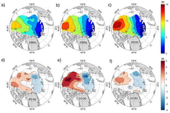
Figure 3.
(a–c) Distributions of liquid freshwater content and their differences (d–f) in the upper 100 m layer in the Arctic Ocean for the 1990s, 2000s, and 2010s.
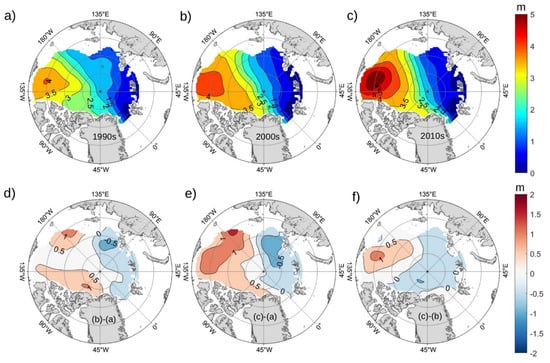
Figure 4.
(a–c) Distributions of liquid freshwater content and their differences (d–f) in the upper halocline layer (50–100 m) in the Arctic Ocean for the 1990s, 2000s, and 2010s.
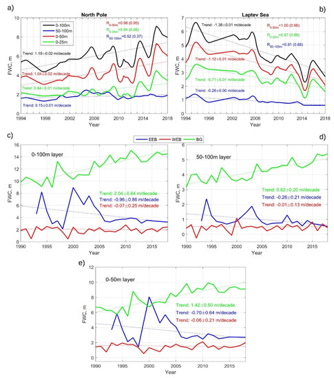
Figure 5.
Time series of freshwater content (FWC) for different ocean layers estimated in the North Pole and Laptev Sea slope regions (a,b), in the western and eastern Eurasian Basins, and in the Beaufort Gyre (c–e). Linear trends are shown by dashed color lines. In (a,b), correlation coefficients (R) between FWC in the upper 100 m layer and FWC for other layers are shown by color numbers. Numbers in brackets in (a,b) show correlations calculated using detrended series. Linear trends in all series are shown by dashed lines.
The comparison revealed that FWC in the upper halocline layer (FWC50–100) comprises ~20% of that in the 100 m layer, as evidenced by the ratio of the record mean FWC in the central Arctic and in the EEB. A slightly higher contribution (up to 30%) for the 50–100 m layer was estimated in the Canada Basin due to deeper penetration of surface freshening into the water column (Figure 5). This 20–30% contribution is smaller than we can expect taking into account a two-fold difference in the vertical extensions of these layers. The smaller contribution of the 50–100 m layer to the net FWC balance confirms that the essential processes for regulating freshwater balance are concentrated in the upper 50 m ocean layer. Approximately the same contribution of 20% for the 50–100 m layer was found in comparing FWC variance; thus, the contribution of this layer to the variability of freshwater content is approximately the same as the contribution to the average value of freshwater content.
3.2. A Pan-Arctic FWC Pattern
Further, we calculated mean FWC in the deep (>100 m) Arctic Ocean interior for the 1990s, 2000s and 2010s. Since the 1990s, the total volume of freshwater in the 0–100 m layer has varied in a wide range from 46,000 to 74,000 km3, which is equivalent to the 5.2–6.4 m range in terms of freshwater content (here and afterward, we will use FWC100 to indicate freshwater content in the 100 m layer; Table 1). Calculated variations in the volume of freshwater were in response to natural variability in the Arctic climate system, but some changes are due to the spatial extension in the area covered by hydrographic observations in the last two decades. The latter is sufficiently important since the area of the Arctic Ocean for which the FWC interpolation was possible in the 2000s and the 2010s differ from that in the 1990s by >30%. To address uncertainties due to different data coverage, we also calculated FWC for the coinciding part of the Arctic Ocean where spatial interpolation was possible for all three decades. Those statistics are provided in Table 1 in brackets.

Table 1.
Decadal freshwater content (FWC) in the Arctic Ocean stored in the upper 100 m layer in the 1990s–2010s. Numbers in brackets represent FWC calculated for the limited area with the restored FWC values for all three decades. The values after plus-minus sign indicate the standard error (SE) of the mean (SE = SD/
, where N is the number of observations used for averaging). SD stands for the standard deviation.
A pan-arctic FWC100 pattern in all decades reflects the influence of two primary sources of inflow of salty or fresh waters into the Arctic basin—the Atlantic and Pacific inflows ([17,35]; Figure 3). Specifically, the influence of the AW inflow is confirmed by high pattern correlations (R > 0.9) calculated for the decadal distributions of FWC100 and the positions of the upper boundary of the AW layer determined using a zero-degree isotherm, similar to that reported by Alekseev et al. [7]. According to this global pattern, FWC gradually increases from Fram Strait—the main gateway for the salty (S > 34.9; [36]) AW to penetrate the Arctic—toward the Canada basin. Further redistribution of the high-salinity water from the Atlantic predominantly in the EB interior produces lower FWC100 in the eastern sector (longitude < 180° E) of the Arctic Ocean compared to that typical for the Canada Basin (see for example, typical salinity profiles for the major Arctic Basins shown in Figure 1c). The lowest FWC100 (<1 m) was found in the western part of the EB in the sector adjacent to the Greenland Sea and western Fram Strait (see Figure 1 for geographical locations) indicating that the average salinity in the upper 100 m layer was close to Sref.
The most significant accumulation of freshwater in the Arctic Ocean was registered in the Canada Basin in response to advection of the relatively fresh (31.0 < S < 34.0; [5]) water from the Pacific Ocean through Bering Strait and redistribution of the Siberian and Canadian river runoff. An additional mechanism favorable for freshwater accumulation in the Canada Basin is the anticyclonic circulation and associated Ekman convergence of surface currents, which makes the Beaufort Gyre the largest freshwater reservoir in the Arctic Ocean [8,9,37,38]. As a result, the storage of freshwater in the upper 100 m layer there was as large as ~15 m (Figure 3). The area located along the trajectory of transpolar drift from the east Siberian coast toward Fram Strait serves as a transit zone separating the Arctic Ocean interior for two basins with very different trends in FWC changes (see Section 3.3 for details).
3.3. FWC Variability in the 1990s–2010s
3.3.1. FWC Differences between Decades
At time scales comparable to the length of our records (29 years), FWC variability in the upper 100 m layer showed two opposite tendencies in the Eurasian and Canada basins of the Arctic Ocean. To attest them, we looked firstly at decadal distributions of FWC differences (Figure 3 and Figure 4). Those differences were calculated by subtracting the decadal FWC fields for each pair of the decades (i.e., the 2000s–1990s, 2010s–1990s, and 2010s–2000s) shown in Figure 3a–c and Figure 4a–c. The calculated FWC differences suggest an increased freshwater storage in the Canada Basin alongside freshwater reduction in the upper and halocline layers in the EB. These two tendencies are seen in the differences of the FWC100 in the 2000s relative to the 1990s and most pronounced when compared the 1990s and 2010s (Figure 3e). For the upper 100 m layer, the largest difference in the decadal mean FWC100 (>4 m) was concentrated around the center of the anticyclonic gyre in the Beaufort Sea, gradually decreasing toward the gyre’s periphery. Traces of positive FWC anomalies were also found along the Canadian continental slope toward Fram Strait, indicating a possible trajectory for freshwater release from the Beaufort Gyre into the Nordic Seas. Most likely, the strong anticyclonic atmospheric circulation over the BG in the 2010s, which is favorable for the storage of freshwater in the Canada Basin, may mediate freshwater release along the Canadian continental slope (e.g., [39]).
In the EB, the tendency observed was opposite and the FWC100 demonstrated negative differences if calculated relative to the 1990s (the earliest decade used in our analysis). The strongest negative differences (>2 m) were found in the eastern part of the EB between 110° E and 130° E meridians in the 2010s (Figure 3e). The increase in the content of freshwater in the 0–100 layer in the Canadian sector of the Arctic Ocean and the decrease in the EB remained unchanged when analyzing decadal changes in the upper halocline layer (50–100 m; Figure 4), suggesting that the mechanisms responsible for the basin-wide FWC changes in both layers are similar in nature.
3.3.2. Linear Trends
In line with decadal distributions of FWC anomalies, FWC in the Beaufort Sea showed a positive trend of 2.04 ± 0.64 m per decade, suggesting increased accumulation of freshwater over the last three decades (Figure 5; here and throughout the text, the numbers after the plus or minus sign indicate the 95% confidence intervals evaluated using Student’s t-test). This tendency results in a cumulative increase in freshwater storage of ~5 m since 1990, which is equivalent to ~12,500 km3 for the entire BG region. The linear trend in the BG FWC dominates over the interannual and year-to-year changes so that its contribution describes ~60% of the total FWC variability in the region. The freshening of the upper layer in the Canada Basin spreads through the extensive area, and the positive FWC trends were also found in the Makarov and the central Arctic basins (e.g., Figure 5a). For example, in the central Arctic Basin (the North Pole area), FWC gradually increased from the beginning of the 1990s with an average rate of ~1.2 m/decade. This increase results in the rise of the liquid freshwater content from 4.5 to 7.9 m.
In contrast to the increased freshwater accumulation in the Canada Basin, the amount of freshwater in the EB and particularly in its eastern sector demonstrated negative trends of ~1 m/decade (Figure 5c). The FWC100 decrease in the EEB since 1990 was as large as 2.5 m (from 6 to 3.5 m) or ~2700 km3; however, the rates of FWC changes were not persistent and the most drastic changes in the freshwater balance occurred between 2000 and 2005. Most likely, these changes were manifestations of the continuing salinization of the upper layer in the Atlantic sector of the Arctic Ocean, reported for the EB by Polyakov et al. [18,23]. After 2005, the absolute rate of FWC100 changes substantially reduced (Figure 5c). The contribution of linear trends in the EEB to the total FWC variability was less significant compared to the BG and did not exceed 20%. This suggests a stronger role for variability at shorter (annual and interannual) time scales.
In the WEB, FWC trends are relatively small (−0.1 m/decade) and statistically not distinguished from zero for all layers (i.e., 0–50 m, 0–100 m, and 50–100 m; Figure 5c–e). The lack of significant trends in that sector of the Arctic Ocean indicates that the reasons behind the net FWC decrease in the entire EB are not directly connected to the inflows of the AW and should be found in the Arctic Ocean interior. Otherwise, we would expect the rise of salinity in the upper 100 m layer in the WEB and along the AW pathway through the EB.
For the regions with significant trends, their signs for the FWC in the 50–100 m layer agreed with those made for the 0–100 m layer, although the absolute values of FWC50–100 were smaller (Figure 5d). Specifically, in the EEB, the FWC50–100 negative trend was ~3.6 times smaller compared to that in the upper 100 m layer (−0.26 and −0.96 m/decade, respectively). The agreement of trend signs and the weakening of their amplitudes with depth suggest the downward propagation of the surface salinity signal that causes large-scale FWC changes whose traces can be found at deeper levels (>100 m) in the lower halocline and even in the upper Atlantic layer (not shown).
3.4. Properties of the Atlantic Water Layer
The intensity of the AW inflow and its thermohaline properties determine advective heat and salt transports. Those transports are two significant factors at play to establish the salt and heat content of the intermediate layer in the Arctic Basin (e.g., [28,40,41,42]). We evaluated changes in the thermohaline properties of the intermediate AW to attest their possible link with processes of freshwater changes in the upper ocean. In that evaluation, we utilized reconstructed time vs. depth diagrams of T and S for the same key regions in the EB that were used in Section 3.2 to estimate FWC100 (Figure 6). Specifically, the calculated T and S arrays were utilized to identify positions of the AW boundaries and to look at variations of water temperature and salinity inside the AW layer (Figure 7). In our study, the upper and lower AW boundaries were determined by the position of a zero-degree isotherm, and the AW core temperature (AWCT) was derived as the maximal temperature in the layer limited by those boundaries.
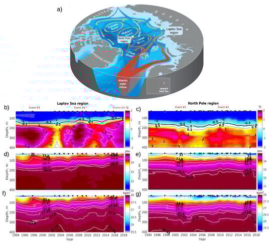
Figure 6.
(a) Circulation of surface water (blue arrows) and intermediate Atlantic Water (AW, red arrows) in the main basins of the Arctic Ocean (adopted from Polyakov et al. 2011). Depth vs. time plot of temperature (b,c), salinity (d,e), and potential density (f,g) in the upper 400 m layer in the Laptev Sea and North Pole regions in 1994–2018. The black line in (b,c) shows the position of AW upper boundary identified using a zero-degree isotherm. Black triangles on the top of each panel indicate the time of CTD profiling.
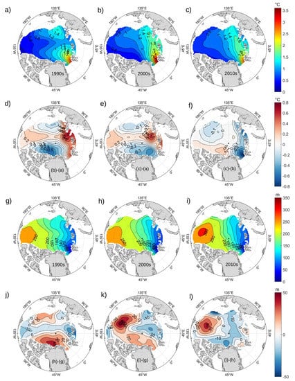
Figure 7.
Decadal distributions of AW core temperatures (a–c, °C) and depths of the upper AW boundary (g–i) in the 1990s, 2000s, and 2010s, and their differences (d–f,j–l)).
3.4.1. AW Core Temperatures
The reconstructed temperature diagrams at the LS slope and the NP regions show coordinated changes in the AW layer in both regions with a time lag of about 2 years (the LS region leads; Figure 6a). Those changes are clearly seen in the form of warm and salt pulses propagating at the intermediate depths below 150 m. The time lag in 2 years corresponds to the time required for the AW to travel with the pan-Arctic boundary current along the Eurasian continental slope and the Lomonosov Ridge from the LS slope to the central Arctic Basin with a mean speed of 2–3 cm/s [24,43]. Over the Laptev Sea slope, warm pulses were observed in 1998, 2008, and 2018 (Figure 6 and Figure 8). The earliest two were registered near the North Pole ~2 years later in 2000 and 2010. The 2018 pulse was not captured near the North Pole by the CTD observations included in our dataset due to its timing; however, we expect to see its evidence at the North Pole in 2020.
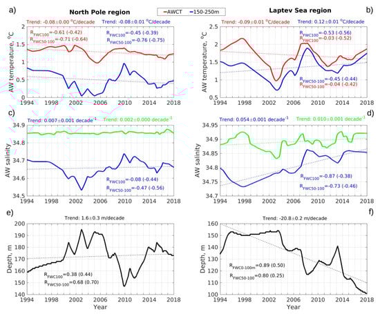
Figure 8.
Time series of Atlantic Water core temperature (AWCT), mean temperature in the 150–250 m layer (a,b), (c,d), respectively; and salinity in the 150–250 m layer (blue line) and in the AW core (green line), and the positions of AW upper boundary (e,f), estimated in the North Pole and Laptev Sea regions. Correlation coefficients (R) between the FWC in the upper 100 m and 50–100 m layers and properties of the Atlantic inflow are shown by color numbers. Numbers in brackets show correlations calculated using the detrended series. Linear trends in all series are shown by dashed lines.
The warm pulses were accompanied by increased AW layer salinity (Figure 6). These linked changes of T an S suggest quite a strong relationship between temperature and salinity anomalies for waters associated with the Atlantic inflows with a high correlation of R > 0.8. Vertical diffusion of heat and salt favors further propagation of T and S anomalies from the AW layer upward to the halocline as evidenced from the coherent temperature changes in the AW core (250–300 m depth), the upper part of the AW layer (150–250m depth), and the lower halocline (70–150m depth; Figure 6 and Figure 8a,b). The warm pulses found in our records manifest the strong influence of advective mechanisms associated with the AW inflows in the formation of warm and salt anomalies and the thermal and salt balance in the EB reported earlier in several studies (e.g., [18,22,44,45,46,47]).
3.4.2. AW Upper Boundary
Alongside the prominent changes in AW temperatures, the position of the upper AW boundary in the Arctic Ocean has undergone significant changes since the 1990s. In the EB, the most substantial rise (~50 m) was revealed over the LS slope (from 150 m in 1995 to 100 m in 2018; Figure 8f). This rise was accompanied by increased average temperature in the upper part of the AW layer (i.e., in the 150–250 m depth range) from ~1.5 °C to 1.8 °C. We speculate that the in-phase changes in the position of the upper AW boundary and AW temperatures in the EB is caused by the vertical redistribution of heat advected with the core of AW and is not due to changes in the volume of the AW inflow.
The rise of the upper AW boundary in the EEB was less evident in the decadal distributions (Figure 7j–l) compared to that estimated from the reconstructed series at the Laptev Sea slope (Figure 8f). The most extensive changes (~20 m) were found over the central Laptev Sea slope in the proximity to the location of our LS region and in the deep Nansen Basin at 85° N latitude (dark blue spots in Figure 7j–l). The reduced decadal differences assume that the most significant changes of AW layer depth have occurred in recent years and were not entirely represented in the decadal distributions. This is confirmed, for example, by more rapid shallowing of the AW boundary from ~140 to ~100 m after 2013 compared to the rise of this boundary observed earlier (Figure 6d).
In opposition to the EEB, the upper AW boundary in the Canada Basin became substantially deeper over the period covered by our dataset (Figure 7g–i). That deepening resulted in more than 50 m increase in the depth for the upper AW boundary (from 250 to 300 m) between the 1990s and the 2010s. This sustained AW deepening in the Canada Basin particularly reflects the response of the intermediate layer of the ocean to the enhanced Ekman convergence due to the anticyclonic atmospheric circulation over the Beaufort Gyre [8,9,38]. The North Pole area is located in a buffer zone between the Canada Basin and the EB. It demonstrates an insignificant change of the AW upper boundary position and less substantial changes in temperatures of the AW core and upper AW layer (Figure 8).
To summarize, our analysis of the thermohaline properties of AW revealed the shift of the upper AW boundary in two opposite directions in the Canada and Eurasian basins. Specifically, we found a rise of the upper AW boundary accompanied by the increase in the core temperature in the eastern EB and deepening of the AW layer in the Canada Basin. At the same time, the areas along the transpolar drift trajectory in the central Arctic and Makarov basin create a transition zone in which changes in thermohaline properties of the Atlantic inflow are much weaker than in the western and eastern Arctic.
3.5. Changes of Density Stratification
Remarkable changes in the thermohaline properties of the upper ocean layer, halocline, and AW layer in the EB and Canada basin altered density stratification over the extensive part of the Arctic Ocean. Following Polyakov et al. [32], to trace changes in stratification, we calculated two parameters (N2 and APE) for the 0–150 m layer (for the layer from the ocean surface to the lower halocline depth) that serve as a climatic proxy for density changes (Figure 9 and Figure 10). Decadal APE differences among decades demonstrate contrasting changes in two major Arctic Ocean basins associated with the strengthening of stratification in the Canada basin (positive APE differences) and general weakening in the EB (negative APE differences). Decadal distributions of APE for the 1990s, 2000s, and 2010s demonstrate similarity in spatial APE and FWC patterns for the corresponding decades. This visible similarity reflects the unique role of salinity in density stratification changes typical for the beta-ocean conditions [48]. The resemblance is also observed for spatial distributions of the decadal APE and FWC anomalies whose pattern correlations varied between decades in the range of 0.6–0.7.
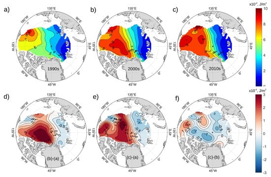
Figure 9.
(a–c) Distributions of the available potential energy (APE × 10−4, J/m2) in the 0–150 m layer in the 1990s, 2000s, and 2010s, and their differences (d–f).
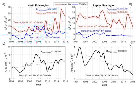
Figure 10.
(a,b) Time series of the mean buoyancy frequency (N2) and (c,d) available potential energy (APE) in the layer between the Atlantic Water and the upper mixed layer estimated in the North Pole and Laptev Sea regions. Correlation coefficients (R) between FWC in the upper 100 m layer and N2 and APE series are shown by color numbers. Numbers in brackets show correlations calculated using the detrended series. Linear trends in all series are shown by dashed lines.
The trend towards stronger stratification of the 0–150m layer in the Canada Basin is consistent with the continued freshening in this region (e.g., [8,12,13,32,49]). Contrasting changes in the upper EB are also consistent with the recent findings of Atlantification in the eastern EB [18]. In our study, we used the term “Atlantification” to attest the shift in the hydrographic conditions (primarily in stratification) and sea ice state to those previously unique to the western Nansen Basin under the influence of inflows from the Atlantic Ocean. The link between density stratification (both N2 and APE) and FWC in the 0–100 m layer was supported by high correlations of time series of these parameters calculated for the two key areas of the Arctic Ocean (Figure 10). For example, for the LS region, this correlation reached 0.92 for the raw APE time series and 0.76 for the series with the removed linear trends. Moreover, the calculated trends in APE and FWC100 also agreed and the decreased freshwater storage in the LS region was concurrent with the decrease in vertical stability of the upper layer. The manifested relationship between the APE and FWC100 was persistent and was also observed in the NP region. Despite the opposite APE and FWC100 trends compared to those found in the EB, the APE and FWC100 correlations between the raw and detrended series were strong (0.74 and 0.64, respectively), suggesting the robustness of the link between FWC and APE.
4. Discussion
4.1. Long-Term FWC Changes
Our analysis revealed two opposite tendencies of FWC changes in the two major basins of the Arctic Ocean—the freshening of the Canada Basin and salinization of the EB and specifically its eastern part (see Section 3). We note that the freshening of the Canada Basin over the last two decades is well documented and captured by the in situ and remote-sensing observations (see, for example, [8] for the detailed discussion). However, crucial differences in the methods used for FWC calculations (e.g., using different Sref, layer thickness, etc.) along with the different geographical regions used make the comparison of our regional FWC estimates with those published in literature a non-trivial task.
Despite the complexity of such a comparison, we claim that the trends estimated in our study for the BG reasonably agree with the estimates made in one of the recent study of FWC using ITP-based observations [8]. For example, based on the annual hydrographic surveys, the authors found that the BG accumulated approximately 6400 km3 of freshwater during 16 years between 2003 and 2018, which is equivalent to the decadal rate of ~4200 km3/decade. Our estimates made with the dataset extended in time suggest a smaller rate of ~2200 km3/decade for the upper 100 m layer evaluated based on the trends from the 1990s. The difference in the FWC trends might be explained by deeper layer used in Proshutinsky et al. [8] for their estimates; the FWC given were made for the layer limited from below by the 34.8 isohaline, i.e., more than 150 m deeper than the lower layer boundary in our calculations (Figure 1c).
The FWC changes observed in the Canada Basin are consistent with the general trend toward freshening evident for the entire Arctic Ocean over the past three decades in which the FWC in the upper 100 m layer has changed by more than 19,000 ± 1000 km3, as evidenced from the comparison of the decadal means (Table 1). However, considering the limited area of the Arctic Ocean, where we have observations in all three decades, those changes were not significant and consisted of ~82,000 ± 12,000 km3. Our estimates agree (within the range on uncertainty) with freshwater changes in the upper ocean layer in the Arctic Basin reported, for example, in [13]. According to the authors, the mean FWC trend calculated using Sref = 35.0 based on monthly gridded fields between 1992 and 2012 was about 600 ± 300 km3 yr−1, which is equivalent to the 16,800 ± 8400 km3 increase in FWC estimated for the period covered by our observations. We speculate that the freshening in the Arctic Ocean will continue since several observation- and model-based studies have suggested an increasing trend in the freshwater supply to the Arctic under warming climate due to increasing atmospheric moisture transport from lower latitudes and increased river runoff [50,51,52,53,54].
The rate of FWC100 changes in the eastern EB (−0.96 m/decade) is approximately two times smaller compared to that found in the BG (Figure 5). Despite the slower rate, the climatic consequences of the observed changes in the FWC seem to be significant because of their interference with the ongoing Atlantification of the eastern Arctic [23]. The FWC in the EB, and especially in its eastern part, is subject to a great influence of atmospheric processes (e.g., [11]). That influence causes a redistribution of river runoff between large-scale basins and regulates the exchange of freshened waters between the shelf regions and the deep ocean [13,55,56]. We speculate that the main reason for the FWC100 decrease in the EEB is a combination of redistribution of low salinity water coming to the basin with river runoff (from Ob’, Enisey, and Lena rivers) and the increased salinity in the halocline layer due to enhanced vertical exchange with the underlying AW layer.
The conclusions about salinization of the upper layer in the EEB and freshening in the Canada Basin in the 2000s–2010s are insensitive to the choice of the lower boundary of the layer used in the FWC calculations. For example, we repeated FWC calculations for the layers limited from below by the depth of mixed layer (FWCMLD) and by the depth of 34.8 psu isohaline (FWC34.8)—an alternative approach used for the FWC calculations (e.g., [8,9,13]). Following Monterey and Levitus [57], the mixed layer depth (MLD) was determined as a depth where potential density differs from the surface density by 0.125 kg/m3.
The calculated FWCMLD and FWC34.8 trends in the EEB and the BG agree with those calculated for the upper 100 m layer (Figure 11; see Figures S8 and S9 in Supplementary Materials for the decadal FWC distributions in these layers). The only difference we found is the positive FWCMLD trend (0.22 ± 0.16 m/decade) in the western sector of the EB compared to the insignificant FWC trend of −0.07 ± 0.25 m/decade within the upper 100 m layer. The consistency of the general trends for the EEB and BG regions estimated for layers with the fixed (FWCMLD and FWC34.8) and variable (FWC50 and FWC100) boundaries suggests that the observed FWC changes are associated with advective and diffusion redistributions of freshwater, whereas the factors affecting the dynamics of the boundaries of these layers (for example, the Ekman pumping associated with long-term changes in atmospheric circulation) likely have a smaller effect.
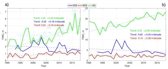
Figure 11.
Time series of freshwater content (FWC; m) in the ocean layers limited by the depth of the mixed layer (a) and the isohaline of 34.8 psu (b) estimated in the western and eastern Eurasian Basins, and in the Beaufort Gyre. Linear trends are shown by dashed color lines.
4.2. Potential FWC Feedback
4.2.1. FWC-Mixing Feedback
Following Polyakov et al. [32], the APE serves as an informative climatic indicator attesting the influence of ocean stratification on diapycnal mixing and concurrent winter ventilation in the lower halocline in the Arctic Ocean. We found that the FWC100 was well correlated with APE estimated in the layer above a zero-degree isotherm. As we mentioned, that isotherm is associated with the position of the upper boundary of the AW layer. The correlation coefficients between FWC100 and APE for the NP area and the LS slope were 0.74 ± 0.18 and 0.92 ± 0.22, respectively, suggesting a strong link between these two parameters. In line with the high correlation, linear FWC trends estimated for the NP and LS areas agreed with those found in APE (Figure 10).
Following the conclusions by Morrison et al. [11] who utilized satellite altimetry from the Gravity Recovery and Climate Experiment (GRACE) and found that the Eurasian river runoff diverted toward the Canada Basin by cyclonic winds over the Eurasian Basin associated with a low Arctic Oscillation index [58], we speculate that recent FWC changes in the EB initiated by the large-scale reconstruction of atmospheric circulation modify the upper ocean stratification in a way that prominently decreases density contrast between the intermediate AW and the upper layer. For instance, such a pattern was observed in the EEB in the 2010s (Figure 6). The weakening density stratification makes plausible further ventilation of the halocline layer and the upper AW during periods of strong winter convection as reported for the western Nansen and eastern Eurasian Basins (e.g., [18,59]). Moreover, the weakening of the insulating effect of the halocline creates favorable conditions for enhanced salt and heat transports from the AW core due to double diffusion [60,61], that results in further salinization of the halocline and shallowing AW boundary. However, the observed increase in the amount of freshwater coming to the eastern Arctic Ocean with river runoff, sea ice melting, and precipitations over the last decades (see [6,50] for estimates) partially masks the upper ocean salinization due to freshwater redistribution between the EB and Canada basin.
The close relationship between density stratification and FWC100 in the EEB (see Section 3 for details) allows us to hypothesize that we found observational evidence for an additional positive feedback. This feedback links changes in the amount of freshwater stored in the upper ocean layer with the intensity of vertical heat and salt exchange in the halocline and upper AW layers. In this feedback, FWC changes arising in response to lateral redistribution of low-salinity melt and riverine waters modify vertical stratification and consequently affect the intensity of vertical heat and salt transports from the underlying ocean layers. Entrainment of saltier waters due to enhanced vertical mixing continues further salinization of the upper ocean layer, closing a positive feedback loop between the FWC and vertical mixing. We should emphasize here that in this feedback, surface salinization and freshening have apparently the leading or even triggering role that is confirmed, for example, by more significant salinity (freshwater) changes observed in the upper 25 m layer compared to the halocline (Figure 5).
In the EEB where the freshwater storage has decreased over the past three decades (Table 1) from 5.2 to 3.6 m (or from 5.1 to 3.6 m for the coinciding area), this mechanism led to a substantial weakening of vertical stratification as seen from distributions of the APE differences in the 0–150 m layer between the 2010s and 1990s (Figure 9e and Figure 10b,d). This decrease in stratification favored stronger vertical exchange with the underlying AW which led to the salinity rise (FWC reducing) in the halocline layer (Figure 5 and Figure 8). It is important that the FWC reduction in the EEB halocline was accompanied by a temperature increase in the upper AW layer, suggesting that the FWC-mixing feedback plays a role not only in the basin-wide salinity changes but also in the establishment of the thermal balance of the halocline. Supporting this, we note that the increased level of vertical mixing and associated increased oceanic heat fluxes in the EEB was documented in recent decades, particularly in [33,62]. Specifically, based on multi-year observations on moorings in the EEB, the authors found a substantial increase in upward oceanic heat flux during the winter season from an average of 3–4 W m−2 in 2007–08 to >10 W m−2 in 2016–18. Taking into account the significant correlation between T and S in the upper AW layer (see Section 3.4.1), this increase should be accompanied by the increased salt fluxes through the halocline.
It is also likely that in the EB, the FWC-vertical mixing feedback works jointly with the ice–ocean heat mechanisms proposed in [18,33] that are driving ongoing Atlantification in the eastern Arctic Ocean. Moreover, stratification changes due to freshwater content decrease may not be the only reason for increased vertical mixing. For example, Polyakov et al. [62], using instrumental records from a set of moorings deployed in the eastern EB in 2004–2018, found that changes in ocean dynamics associated with the two-fold enhancement of semidiurnal tidal and near-inertial currents played a significant role in this process, making a general picture of climatic changes in the EB even more complex.
4.2.2. Variability of the Mixed Layer Depth in the EEB
Direct instrumental observations of mixing in the Arctic Ocean are rare. Instead, to highlight the suggested link between the FWC and mixing intensity, we assessed the strength of winter ventilation—the essential mechanism favorable for vertical mixing in the upper ocean. For that, we calculated the depths of the winter (February–April) mixed layer using available CTD profiles in the eastern EB. The winter oceanographic data were rare in the 1990s; thus, for comparison, we used the 1970s during which the data coverage in the EEB was good to provide reliable MLD statistics.
Our CTD observations captured an increase in the winter MLD in the EEB over the last two decades. Specifically, the decadal mean MLD increased from 24.5 m in the 1970s to 40.5 m in the 2000s and to 44 m in the 2010s, suggesting a near doubling of the winter convection depths and associated mixing increase in these decades (Figure 12). The enhanced penetration of winter mixing in the 2000s and 2010s agrees with the reduced FWC and vertical stratification in the halocline layer in the EB. These changes suggest that under conditions of the “new” Arctic Ocean, the shallow winter convection regime with MLD < 30 m becomes less probable.
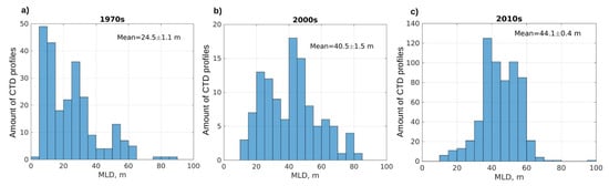
Figure 12.
Probability distribution functions (PDFs) of the winter (February–April) surface mixed layer depth (MLD) for the 1970s (a), 2000s (b), and 2010s (c).
4.3. The Link between the FWC and AW Properties
The potential FWC–vertical exchange feedback partially explains the ongoing changes in the upper AW layers and the lower halocline. For instance, the opposite trends in the FWC100 and the upper boundary of the AW in the Eurasian and Canada basins, along with the visible similarity in spatial patterns of their decadal anomalies, allow us to speculate about their possible connection driven by this feedback. It is evident that the upper part of the AW layer (from the core to the upper AW boundary) and the lower halocline (~70–150 m) in the eastern EB and the central Arctic Ocean became saltier, as evidenced by rising isohalines in the salinity range from 34.5 to 34.85 (Figure 5 and Figure 6) and positive trends in the mean salinity of the upper AW layer in the North Pole and Laptev Sea regions (0.007 ± 0.001 and 0.054 ± 0.001 decade−1, respectively; Figure 8). On average, the isohaline rise at the Laptev Sea slope was about 50 m over the 1994–2018 period that matches the shallowing of AW upper boundary (~50 m). The salinization of the lower halocline in the EB agrees with the decadal FWC anomalies for the 50–100 m layer in the 2000s and 2010s showing a gradual reduction of freshwater content (increased layer-mean salinity) in these decades. Supporting the hypothesis about the influence of AW salinity changes on FWC in the halocline layer, we found moderate negative correlations (R~−0.4; both are significant at the 95% confidence level) between the detrended FWC50–100 series and the average salinity in the upper AW layer (150–250 m layer) in the Laptev Sea and North Pole regions (Figure 8c,d).
In contrast to FWC and the upper AW boundary, the correlations between FWC100 and AW temperatures and salinities in the eastern and the central Arctic Ocean revealed a somewhat inconsistent relationship. For example, the correlation coefficients between the FWC100 with AWCT varied in the range from −0.61 ± 0.25 in the central Arctic Basin to the statistically insignificant value of 0.02 ± 0.25 at the Laptev Sea slopes (Figure 8). However, for the time series with the excluded linear trends, those correlations became close to each other, changing to −0.4 (in all figures, the correlations in brackets indicate the correlations calculated for series after removing linear trends). The link between the detrended AW temperatures and the FWC in the upper halocline layer (FWC50–100) was also high, reaching −0.75 ± 0.05 in the North Pole region. Given the relatively high correlations for the advected temperature and salinity anomalies in the AW layer (Section 3.4), that link suggests the entrainment of warm and saltier AW to the upper halocline in the eastern EB and central Arctic Ocean.
4.4. Limitations of the Analysis
Despite the statistical robustness of our estimates regarding recent FWC changes and trends in the Arctic, our results and calculations are influenced by several limitations. Most of these limitations arise from the limitations of the oceanographic data used in our study and the methods implemented. For the in-depth discussion of the limitations, see Supplementary Materials to this paper.
5. Conclusions
The analysis performed allows us to summarize several conclusions:
Our analysis revealed two opposite tendencies–the freshening in the Canada Basin with the mean rate of 2.0 m/decade and the salinization of the eastern EB at the rate of 0.96 m/decade (Figure 5). The trend estimated for the Canada Basin is persistent and reflects a general tendency towards freshening that has been typical for the Arctic Ocean over the last three decades. In contrast, the FWC100 decrease in the EB since 1990 was less significant by amplitude, and the rates of FWC changes were not persistent so that the most drastic changes in the freshwater balance there occurred between 2000 and 2005.
The most significant FWC changes were captured in the upper 50 m layer (Figure 5e and Figure S7)—within the layer that is critically important to quantify mechanisms of freshwater redistribution in the Arctic Ocean. However, even though that the layer below 50 m contributes only 20% to the net FWC in the 100 m layer, FWC variations in the halocline and the intermediate layers may also be important for reflecting global oceanic processes linked to the advection of waters from polar sectors of the Atlantic and Pacific Oceans (see [23] for details).
Our analysis of the thermohaline properties of AW—the major source of salt and heat for the Polar Regions—revealed the shift of the upper AW boundary in two opposite directions in the Canada and Eurasian basins (Figure 7). Specifically, we documented a 50 m rise of the upper AW boundary accompanied by a 0.5 °C increase in the AW core temperature in the eastern EB and approximately the same strong deepening of the AW layer in the Canada Basin.
The close relationship between APE in the layer above the AW and FWC100 in the eastern EB (Section 3) provides us with evidence of the positive feedback that links the amount of freshwater stored in the upper ocean layer with the intensity of vertical heat and salt exchange in the halocline and upper AW layers. Entrainment of saltier waters from the AW layer due to the enhanced vertical mixing continues further salinization of the upper ocean layer, which was evident in the EB over the last decade. Together with other mechanisms of Atlantification, this feedback creates a complex picture of interactions behind the observed changes in the hydrological and ice regimes of the Eurasian sector of the Arctic.
Supplementary Materials
The following supporting information can be downloaded at: https://www.mdpi.com/article/10.3390/jmse10030401/s1, Section S1: Limitations of the analysis; Figures S1–S6: Yearly distributions of liquid freshwater content in the Arctic Ocean in the 1990s–2010s; Figures S7–S9: Distributions of liquid freshwater content and their differences in the 0–50-m layer, in the mixed layer, and in the layer limited by the depth of 34.8 isohaline in the Arctic Ocean for the decades of the 1990s, 2000s, and 2010s.
Author Contributions
A.V.P. conceived the study and carried out the calculations. A.V.P., G.V.A. and A.V.S. contributed to the analysis of the results and wrote the manuscript. All authors have read and agreed to the published version of the manuscript.
Funding
Analysis presented in this paper was carried out within the framework of the Nansen and Amundsen Basins Observational Program (NABOS) project, with support from the NSF (grants AON-1203473, AON-1338948, and AON-1724523). G.A., A.S. were supported by RFBR grant 18-05-60107 ‘Changes in the freshwater balance of the Arctic Ocean during global warming, their impact on sea ice and amplification of the warming in the Arctic’.
Institutional Review Board Statement
Not applicable.
Informed Consent Statement
Not applicable.
Data Availability Statement
The results of FWC calculations used in this study are available upon request to the authors.
Acknowledgments
We thank the Academic Editor, Lars Chresten Lund-Hansen, and three anonymous reviewers for their valuable comments and help with the manuscript.
Conflicts of Interest
The authors declare no conflict of interest.
References
- Shiklomanov, I.; Shiklomanov, A.; Lammers, R. The Dynamics of River Water Inflow to the Arctic Ocean. In The Freshwater Budget of the Arctic Ocean; Lewis, E.L., Ed.; Kluwer Academic Publishers: Dordrecht, The Netherlands, 2000. [Google Scholar]
- Rachold, V.; Eicken, H.; Gordeev, V.V.; Grigoriev, M.N.; Hubberten, H.-W.; Lisitzin, A.P.; Shevchenko, V.P.; Schirrmeister, L. Modern Terrigenous Organic Carbon Input to the Arctic Ocean. In The Organic Carbon Cycle in the Arctic Ocean; Springer: Berlin/Heidelberg, Germany, 2004; pp. 33–55. [Google Scholar]
- Fichot, C.; Kaiser, K.; Hooker, S.; Amon, R.M.V.; Babin, M.; Bélanger, S.; Walker, S.A.; Benner, R. Pan-Arctic distributions of continental runoff in the Arctic Ocean. Sci. Rep. 2013, 3, 1053. [Google Scholar] [CrossRef] [PubMed]
- Woodgate, R.A.; Aagaard, K.; Weingartner, T.J. Interannual changes in the Bering Strait fluxes of volume, heat and freshwater between 1991 and 2004. Geophys. Res. Lett. 2006, 33, L15609. [Google Scholar] [CrossRef]
- Woodgate, R.A.; Weingartner, T.J.; Lindsay, R. Observed increases in Bering Strait oceanic fluxes from the Pacific to the Arctic from 2001 to 2011 and their impacts on the Arctic Ocean water column. Geophys. Res. Lett. 2012, 39, L24603. [Google Scholar] [CrossRef]
- Carmack, E.C.; Yamamoto-Kawai, M.; Haine, T.W.N.; Bacon, S.; Bluhm, B.A.; Lique, C.; Melling, H.; Polyakov, I.V.; Straneo, F.; Timmermans, M.-L.; et al. Freshwater and its role in the Arctic Marine System: Sources, disposition, storage, export, and physical and biogeochemical consequences in the Arctic and global oceans. J. Geophys. Res. Biogeosci. 2016, 121, 675–717. [Google Scholar] [CrossRef]
- Alekseev, G.V.; Pnyushkov, A.V.; Smirnov, A.V.; Vyazilova, A.E.; Glok, N.I. Influence of Atlantic inflow on the freshwater content in the upper layer of the Arctic basin. Arct. Antarct. Res. 2019, 65, 363–388. [Google Scholar] [CrossRef][Green Version]
- Proshutinsky, A.; Krishfield, R.; Toole, J.M.; Timmermans, M.-L.; Williams, W.; Zimmermann, S.; Yamamoto-Kawai, M.; Armitage, T.W.K.; Dukhovskoy, D.; Golubeva, E.; et al. Analysis of the Beaufort Gyre freshwater content in 2003–2018. J. Geophys. Res. Ocean. 2019, 124, 9658–9689. [Google Scholar] [CrossRef] [PubMed]
- Proshutinsky, A.; Krishfield, R.; Barber, D. Preface to Special Section on Beaufort Gyre Climate System Exploration Studies: Documenting Key Parameters to Understand Environmental Variability. J. Geophys. Res. 2009, 114, C00A08. [Google Scholar] [CrossRef]
- Rawlins, M.A.; Steele, M.; Holland, M.L.; Adam, J.C.; Cherry, J.E.; Francis, J.A.; Groisman, P.Y.; Hinzman, L.D.; Huntington, T.G.; Kane, D.L.; et al. Analysis of the Arctic System for Freshwater Cycle Intensification: Observations and Expectations. J. Clim. 2010, 23, 5715–5737. [Google Scholar] [CrossRef]
- Morison, J.; Kwok, R.; Peralta-Ferriz, C.; Alkire, M.; Rigor, I.; Andersen, R.; Steele, M. Changing Arctic Ocean Freshwater Pathways. Nature 2012, 481, 66–70. [Google Scholar] [CrossRef] [PubMed]
- Rabe, B.; Karcher, M.; Schauer, U.; Toole, J.; Krishfield, R.; Pisarev, S.; Kauker, F.; Gerdes, R.; Kikuchi, T. An assessment of Arctic Ocean freshwater content changes from the 1990s to 2006–2008. Deep-Sea Res. Part I Oceanogr. Res. Pap. 2011, 58, 173–185. [Google Scholar] [CrossRef]
- Rabe, B.; Karcher, M.; Kauker, F.; Schauer, U.; Toole, J.M.; Krishfield, R.A.; Pisarev, S.; Kikuchi, T.; Su, J. Arctic Ocean liquid freshwater storage trend 1992–2012. Geophys. Res. Lett. 2014, 41, 961–968. [Google Scholar] [CrossRef]
- Rudels, R.; Jones, E.P.; Schauer, U.; Ericksson, P. Atlantic sources of the Arctic Ocean surface and halocline waters. Polar Res. 2004, 23, 181–208. [Google Scholar] [CrossRef]
- Korhonen, M.; Rudels, B.; Marnela, M.; Wisotzki, A.; Zhao, J.P. Time and space variability of freshwater content, heat content and seasonal ice melt in the Arctic Ocean from 1991 to 2011. Ocean Sci. 2012, 9, 2621–2677. [Google Scholar] [CrossRef]
- Zakharov, V.F. Ice of the Arctic and Current Natural Processes; Gidrometeoizdat: Leningrad, Russia, 1981; p. 136. (In Russian) [Google Scholar]
- Aagaard, K.; Carmack, E.C. The role of sea ice and fresh water in the Arctic circulation. J. Geophys. Res. Ocean. 1989, 94, 14485–14498. [Google Scholar] [CrossRef]
- Polyakov, I.V.; Pnyushkov, A.; Alkire, M.; Ashik, I.; Baumann, T.; Carmack, E.; Goszczko, I.; Guthrie, J.; Ivanov, V.; Kanzow, T.; et al. Greater role for Atlantic inflows on sea-ice loss in the Eurasian Basin of the Arctic Ocean. Science 2017, 356, 285–291. [Google Scholar] [CrossRef] [PubMed]
- Serreze, M.C.; Stroeve, J. Arctic sea ice trends, variability and implications for seasonal ice forecasting. Philos. Trans. Math. Phys. Eng. Sci. 2015, 373, 20140159. [Google Scholar] [CrossRef] [PubMed]
- Polyakov, I.V.; Alexeev, V.; Belchansky, F.I.; Dmitrenko, I.A.; Ivanov, V.; Kirillov, S.; Korablev, A.; Steele, M.; Timokhov, L.A.; Yashayaev, I. Arctic Ocean freshwater changes over the past 100 year and their causes. J. Clim. 2008, 21, 364–384. [Google Scholar] [CrossRef]
- Yamamoto-Kawai, M.; McLaughlin, F.A.; Carmack, E.C.; Nishino, S.; Shimada, K.; Kurita, N. Surface freshening of the Canada Basin, 2003–2007: River runoff versus sea ice meltwater. J. Geophys. Res. 2009, 114, C00A05. [Google Scholar] [CrossRef]
- Polyakov, I.V.; Bhatt, U.S.; Walsh, J.E.; Abrahamsen, E.P.; Pnyushkov, A.V. Recent oceanic changes in the Arctic in the context of longer term observations. Ecol. Appl. 2013, 23, 1745–1764. [Google Scholar] [CrossRef] [PubMed]
- Polyakov, I.V.; Alkire, M.B.; Bluhm, B.A.; Brown, K.A.; Carmack, E.C.; Chierici, M.; Pnyushkov, A.V.; Ingvaldsen, R.B.; Pnyushkov, A.V.; Slagstad, D.; et al. Borealization of the Arctic Ocean in response to anomalous advection from sub-Arctic seas. Front. Mar. Sci. 2020, 7, 491. [Google Scholar] [CrossRef]
- Pnyushkov, A.; Polyakov, I.; Ivanov, V.; Aksenov, Y.; Coward, A.; Janout, M.; Rabe, B. Structure and variability of the boundary current in the Eurasian Basin of the Arctic Ocean. Deep-Sea Res. Part I Oceanogr. Res. Pap. 2015, 101, 80–97. [Google Scholar] [CrossRef]
- Pnyushkov, A.; Polyakov, I.V.; Padman, L.; Nguyen, A.T. Structure and dynamics of mesoscale eddies over the Laptev Sea continental slope in the Arctic Ocean. Ocean Sci. 2018, 14, 1329–1347. [Google Scholar] [CrossRef]
- Pnyushkov, A.; Polyakov, I.; Rember, R.; Ivanov, V.; Alkire, M.B.; Ashik, I.; Baumann, T.M.; Alekseev, G.; Sundfjord, A. Heat, salt, and volume transports in the eastern Eurasian Basin of the Arctic Ocean from 2 years of mooring observations. Ocean Sci. 2018, 14, 1349–1371. [Google Scholar] [CrossRef]
- Pickart, R.S. Shelfbreak circulation in the Alaskan Beaufort Sea: Mean structure and variability. J. Geophys. Res. 2004, 109, C04024. [Google Scholar] [CrossRef]
- Rudels, B.; Anderson, L.G.; Jones, E.P. Formation and evolution of the surface mixed layer and halocline of the Arctic Ocean. J. Geophys. Res. 1996, 101, 8807–8821. [Google Scholar] [CrossRef]
- Padman, L.; Dillon, T.M. Vertical heat fluxes through the Beaufort Sea thermohaline staircase. J. Geophys. Res. 1987, 92, 10799–10806. [Google Scholar] [CrossRef]
- D’Asaro, E.A.; Morison, J.H. Internal waves and mixing in the Arctic Ocean. Deep-Sea Res. Part A Oceanogr. Res. Pap. 1992, 39, S459–S484. [Google Scholar] [CrossRef]
- Lorenz, E.E. Available Potential Energy and the Maintenance of the General Circulation. Tellus 1955, 7, 157–167. [Google Scholar] [CrossRef]
- Polyakov, I.V.; Pnyushkov, A.; Carmack, E.C. Stability of the arctic halocline: A new indicator of arctic climate change. Environ. Res. Lett. 2018, 13, 125008. [Google Scholar] [CrossRef]
- Polyakov, I.V.; Rippeth, T.P.; Fer, I.; Alkire, M.B.; Baumann, T.M.; Carmack, E.C.; Ingvaldsen, R.; Ivanov, V.V.; Janout, M.; Lind, S.; et al. Weakening of Cold Halocline Layer Exposes Sea Ice to Oceanic Heat in the Eastern Arctic Ocean. J. Clim. 2020, 33, 8107–8123. [Google Scholar] [CrossRef]
- MATLAB; Version R2015b; The MathWorks Inc.: Natick, MA, USA, 2015.
- Jones, E.P.; Anderson, L.G.; Jutterström, S.; Mintrop, L.; Swift, J.H. Pacific freshwater, river water and sea ice meltwater across Arctic Ocean basins: Results from the 2005 Beringia Expedition. J. Geophys. Res. 2008, 113, C08012. [Google Scholar] [CrossRef]
- Schauer, U.; Fahrbach, E.; Osterhus, S.; Rohardt, G. Arctic warming through the Fram Strait: Oceanic heat transport from 3 years of measurements. J. Geophys. Res. 2004, 109, C06026. [Google Scholar] [CrossRef]
- Treshnikov, A.F.; Baranov, G.I. Water Circulation in the Arctic Basin; Israel Program for Scientific Translations: Jerusalem, Israel, 1973. [Google Scholar]
- Armitage, T.W.K.; Manucharyan, G.E.; Petty, A.A.; Kwok, R.; Thompson, A.F. Enhanced eddy activity in the Beaufort Gyre in response to sea ice loss. Nat. Commun. 2020, 11, 761. [Google Scholar] [CrossRef] [PubMed]
- Zhang, J.; Weijer, W.; Steele, M.; Cheng, W.; Verma, T.; Veneziani, M. Labrador Sea freshening linked to Beaufort Gyre freshwater release. Nat. Commun. 2021, 12, 1229. [Google Scholar] [CrossRef] [PubMed]
- Rudels, B. Arctic Ocean circulation and variability—Advection and external forcing encounter constraints and local processes. Ocean Sci. 2012, 8, 261–286. [Google Scholar] [CrossRef]
- Schauer, U.; Rudels, B.; Jones, E.P.; Anderson, L.G.; Muench, R.D.; Björk, G.; Swift, J.H.; Ivanov, V.; Larsson, A.-M. Confluence and redistribution of Atlantic water in the Nansen, Amundsen and Makarov basins. Ann. Geophys. 2002, 20, 257–273. [Google Scholar] [CrossRef]
- Häkkinen, S.; Proshutinsky, A. Freshwater content variability in the Arctic Ocean. J. Geophys. Res. 2004, 109, C03051. [Google Scholar] [CrossRef]
- Pnyushkov, A.; Polyakov, I.; Ivanov, V.; Kikuchi, T. Structure of the Fram Strait Branch of the Boundary Current in the Eurasian Basin of the Arctic Ocean. Polar Sci. 2013, 7, 53–71. [Google Scholar] [CrossRef][Green Version]
- Quadfasel, D.; Sy, A.; Wells, D.; Tunik, A. Warming in the Arctic. Nature 1991, 350–385. [Google Scholar] [CrossRef]
- Polyakov, I.V.; Beszczynska, A.; Carmack, E.C.; Dmitrenko, I.A.; Fahrbach, E.; Frolov, I.E.; Gerdes, R.; Hansen, E.; Holfrot, J.; Ivanov, V.V.; et al. One more step toward a warmer Arctic. Geophys. Res. Lett. 2005, 32, L17605. [Google Scholar] [CrossRef]
- Dmitrenko, I.A.; Polyakov, I.V.; Kirillov, S.A.; Timokhov, L.A.; Frolov, I.E.; Sokolov, V.T.; Simmons, H.L.; Ivanov, V.V.; Walsh, D. Toward a Warmer Arctic Ocean: Spreading of the Early 21st Century Atlantic Water Warm Anomaly along the Eurasian Basin Margins. J. Geophys. Res. 2008, 113, C05023. [Google Scholar] [CrossRef]
- Pnyushkov, A.V.; Polyakov, I.V.; Alekseev, G.V.; Ashik, I.M.; Baumann, T.M.; Carmack, E.C.; Ivanov, V.V.; Rember, R. A Steady Regime of Volume and Heat Transports in the Eastern Arctic Ocean in the Early 21st Century. Front. Mar. Sci. 2021, 8, 705608. [Google Scholar] [CrossRef]
- Carmack, E.C. The alpha/beta ocean distinction: A perspective on freshwater fluxes, convection, nutrients and productivity in high-latitude seas. Deep-Sea Res. Part II Top. Stud. Oceanogr. 2007, 54, 2578–2598. [Google Scholar] [CrossRef]
- McPhee, M.G.; Proshutinsky, A.; Morison, J.H.; Steele, M.; Alkire, M.B. Rapid change in freshwater content of the Arctic Ocean. Geophys. Res. Lett. 2009, 36, L10602. [Google Scholar] [CrossRef]
- Haine, T.W.N.; Curry, B.; Gerdes, R.; Hansen, E.; Karcher, M.; Lee, C.; Rudels, B.; Spreen, G.; de Steur, L.; Stewart, K.D.; et al. Arctic freshwater export: Status, mechanisms, and prospects. Glob. Planet. Change 2015, 125, 13–35. [Google Scholar] [CrossRef]
- Peralta-Ferriz, C.; Woodgate, R.A. Seasonal and interannual variability of pan-Arctic surface mixed layer properties from 1979 to 2012 from hydrographic data, and the dominance of stratification for multiyear mixed layer depth shoaling. Prog. Oceanogr. 2015, 134, 19–53. [Google Scholar] [CrossRef]
- Zhang, X.; Zhang, J.; He, J.; Polaykov, I.; Gerdes, R.; Inoue, J.; Wu, P. Enhanced poleward moisture transport and amplified northern high-latitude wetting trend. Nat. Clim. Change 2013, 3, 47–51. [Google Scholar] [CrossRef]
- Fu, W.W.; Moore, J.K.; Primeau, F.W.; Lindsay, K.; Randerson, J.T. A Growing Freshwater Lens in the Arctic Ocean with Sustained Climate Warming Disrupts Marine Ecosystem Function. J. Geophys. Res. Biogeosci. 2020, 125, e2020JG005693. [Google Scholar] [CrossRef]
- Wang, Q.; Danilov, S.; Sidorenko, D.; Wang, X. Circulation Pathways and Exports of Arctic River Runoff Influenced by Atmospheric Circulation Regimes. Front. Mar. Sci. 2021, 8, 707593. [Google Scholar] [CrossRef]
- Janout, M.A.; Aksenov, Y.; Hölemann, J.A.; Rabe, B.; Schauer, U.; Polyakov, I.V.; Bacon, S.; Coward, A.C.; Karcher, M.A.; Lenn, Y.-D.; et al. Kara Sea freshwater transport through Vilkitsky Strait: Variability, forcing, and further pathways toward the western Arctic Ocean from a model and observations. J. Geophys. Res. Ocean. 2015, 120, 4925–4944. [Google Scholar] [CrossRef]
- Janout, M.A.; Hölemann, J.; Laukert, G.; Smirnov, A.; Krumpen, T.; Bauch, D.; Timokhov, L. On the Variability of Stratification in the Freshwater-Influenced Laptev Sea Region. Front. Mar. Sci. 2020, 7, 622416. [Google Scholar] [CrossRef]
- Monterey, G.I.; Levitus, S. Seasonal Variability of Mixed Layer Depth for the World Ocean. In NOAA Atlas NESDIS 14; NOAA: Washington, DC, USA, 1997; p. 5. [Google Scholar]
- Thompson, D.W.J.; Wallace, J. The Arctic Oscillation signature in the wintertime geopotential height and temperature fields. Geophys. Res. Lett. 1998, 25, 1297–1300. [Google Scholar] [CrossRef]
- Ivanov, V.; Alexeev, V.; Koldunov, N.V.; Repina, I.; Sandø, A.B.; Smedsrud, L.H.; Smirnov, A. Arctic Ocean Heat Impact on Regional Ice Decay: A Suggested Positive Feedback. J. Phys. Oceanogr. 2016, 46, 1437–1456. [Google Scholar] [CrossRef]
- Shibley, N.C.; Timmermans, M.-L.; Carpenter, J.R.; Toole, J.M. Spatial variability of the Arctic Ocean’s double-diffusive staircase. J. Geophys. Res. Ocean. 2017, 122, 980–994. [Google Scholar] [CrossRef]
- Polyakov, I.; Padman, L.; Lenn, Y.; Pnyushkov, A.; Rember, R.; Ivanov, V. Eastern Arctic Ocean diapycnal heat fluxes through large double-diffusive steps. J. Phys. Oceanogr. 2019, 49, 227–246. [Google Scholar] [CrossRef]
- Polyakov, I.V.; Rippeth, T.P.; Fer, I.; Baumann, T.M.; Carmack, E.C.; Ivanov, V.V.; Pnyushkov, A.V.; Rember, R. Intensification of Near-Surface Currents and Shear in the Eastern Arctic Ocean. Geophys. Res. Let. 2020, 46, e2020GL089469. [Google Scholar] [CrossRef]
Publisher’s Note: MDPI stays neutral with regard to jurisdictional claims in published maps and institutional affiliations. |
© 2022 by the authors. Licensee MDPI, Basel, Switzerland. This article is an open access article distributed under the terms and conditions of the Creative Commons Attribution (CC BY) license (https://creativecommons.org/licenses/by/4.0/).