Experimental and Numerical Studies of Cloud Cavitation Behavior around a Reversible S-Shaped Hydrofoil

Abstract

The S-shaped hydrofoil is often used in the design of reversible machinery due to its centrally symmetrical camber line. The objective of this paper is to study the influence of cloud cavitation on the flow structure and the unsteady characteristics of lift and drag around an S-shaped hydrofoil via experimental tests and numerical simulations. In the experimental component, the tests were carried out in a cavitation tunnel and a high-speed camera was used to record the cavitation details around the S-shaped hydrofoil with different cavitation numbers. The experimental results show that sheet cavitation gradually transforms into cloud cavitation with a decrease in the inlet cavitation number, the maximum cavity length increases faster after the occurrence of cloud cavitation, and the shedding cycle time of cloud cavitation gradually increases with a decrease in the inlet cavitation number. In the numerical component, the numerical results are in good agreement with the experimental data. The numerical results show that the movement of the re-entrant jet is the main factor for the formation of the cloud cavitation around the S-shaped hydrofoil. The shedding cloud cavity induces the U-shaped vortex structure around the S-shaped hydrofoil, and it produces a higher vorticity distribution around the cavity. The periodic motion of cloud cavity causes the unsteady fluctuation of the lift–drag coefficient of the S-shaped hydrofoil, and because of the unique pressure distribution characteristics of the S-shaped hydrofoil, the lift and drag coefficient appeared as two peaks in one typical cycle of cloud cavitation.

1. Introduction

Cavitation is a phenomenon that occurs inside a liquid when the pressure is lower than the saturated vapor pressure [1]. The developmental stage of cavitation can be divided into four stages: cavitation inception, sheet cavitation, cloud cavitation, and super cavitation [2]. The cloud cavitation process is produced by the instability fracture of sheet cavitation has obvious periodicity, which is easy to induce vibration, noise, erosion and other problems in hydraulic machinery [3,4].

Cloud cavitation is a complex periodic flow that includes phase–change, vortex, and flow separation and it attracts many research studies that use experiments and numerical simulations. In experimental tests, Knapp et al. [5] discovered the existence of the re-entrant jet in the study of cloud cavitation around an axisymmetric body; Kubota et al. [6] selected laser Doppler anemometry (LDA) and a high-speed camera (HSC) to collect the unstable flow of cloud cavitation around a foil. The cloud cavitation structure has an obvious three-dimensional stretching effect, and there is an obvious vortex concentration center in its center. The re-entrant jets close to the hydrofoil are the main cause of the formation of cloud cavitation. By placing a lateral obstacle in the hydrofoil, Kawanami et al. [7] successfully prevented the re-entrant jets and controlled the shedding of the sheet cavitation. Wang et al. [8] studied four different cavitation developmental stages of 2-D Clark-Y hydrofoil through high-speed observation and Laser Doppler Velocimetry (LDV). During the cloud cavitation stage, the re-entrant jets and the large-scale cloud that leads the lift and drag coefficients reach minimum and maximum. In order to study the complex structure of cavitation flow, Foeth et al. [9,10] designed a twisted hydrofoil and found that rationale for the main shedding and the secondary shedding in the collapse of a cloud cavity. They identified the re-entrant jets as the main factor that caused the shedding of sheet cavitation; the side jet induced the secondary shedding of the cavitation tail. Seyki et al. [11] studied the behavior of the sheet cavity phenomenon around a NACA0015 hydrofoil by increasing or decreasing the angle of attack (AOA). By comparing the cavity lengths with angles of attack changing from zero to twenty and twenty to zero, they observed a different hysteresis effect on the cavity length.

In the past few decades, computational fluid dynamic methods have been applied to further study the evolution of the cavitating flow to solve the limitations of the flow field measurements in the experiment. Morgut et al. [12] compared different cavitation models [13,14,15] to verify the accuracy and the stability of the model of the mass transfer of a two-dimensional sheet cavitation around NACA66 (MOD) and NACA0009. Ji et al. [16] used PANS turbulence model and modified the ratio between liquid density and vapor density in the cavitation model to simulate the twice cavitating flow around a 3D twisted hydrofoil. They used the Q-criterion with the value of 200 to describe a horseshoe shaped vortex. Huang et al. [17] combined the characteristics of the filter-based model (FBM) and the density correction model (DCM), and they proposed the filter-based density correction model (FBDCM) to better predict the attached cavity length and the cavitation flow details. Wang et al. [18] adopted the adaptive mesh refinement (AMR) method to successfully improve the accuracy of the coarse mesh in numerical simulations and to successfully simulate the multi-scale cavity structures and the reverse flow. To study the vortex around the shedding cloud, Ji et al. [19] used the modified RNG turbulence model and they predicted cavity structures and the frequency of cloud shedding consistent with the results of the experiment. They used the vorticity transport equation to show how cavitation affects the vorticity distribution, and they analyzed the contribution of vorticity components to vorticity. By analyzing the vorticity transport equation, Huang et al. [20] concluded the vortex structure had a correlation with the shedding cloud. The process of cloud cavitation has changed the frequency of vortices around the Clark-Y and substantially increased the velocity fluctuation. Zhang et al. [21] used the LES model and Zwart cavitation model to study the different stages of cavitation flow patterns around the Tulin foil. The results of the numerical simulation compared well with the experimental observations, and the cavitating vortex at the trailing edge of the foil had a regular vortex shape and a clear boundary between the vortex structures. Yan et al. [22] designed two foils based on external streamline features. They compared the lift–drag characteristics of the two bionic hydrofoils in detail and analyzed the leading-edge vortices of the bionic hydrofoils using the vorticity transport equation. Pendar et al. [23] conducted numerical calculations on hydrofoil with different leading-edge sinusoidal wave lengths, which successfully prevented boundary layer deflow at the leading edge and reduced the unsteady fluctuation of hydrofoil performance. Movahedian et al. [24] calculated the cloud cavitation flow around the 3D-twisted NACA 16,012 hydrofoil. They analyzed the multiple shedding phenomenon and the pressure pulsation around the hydrofoil.

The S-shaped foils are always used in the design of various reversible fluid machines, such as reversible air fans, pump-turbines, and reversible axial-flow pumps [25,26,27]. Ramachandran et al. [28] studied the change of lift coefficient, the drag coefficient, and the pressure distribution of four fully reversible S-shaped foils with different maximum camber values in the cascade. Chacko et al. [29] discussed the lift–drag coefficients of the reversible hydrofoil with different cut-off trailing edges. They summarized the optimal shape and length of the trailing edge on the forward and the reverse flow conditions, which provided a basis for the asymmetric S-shaped hydrofoil design.

According to past works, the research on S-shaped hydrofoils mainly focuses on the steady lift–drag characteristics and the surface pressure distribution, but there is basically no research on cavitation characteristics or the characteristics of the unsteady flow around the S-shaped hydrofoil. In addition, the unique shape of the S-shaped hydrofoil leads to lower lift than conventional foils (NACA66 (Mod), Clark-Y) at the same angle of attack. In the design process of reversible hydro-machinery, it is necessary to increase the angle of attack of the S-shaped hydrofoil to increase lift, which easily induces cloud cavitation. In our research, we analyze the dynamic of cloud cavitation around S-shaped hydrofoils at the angle of attack α = 6° corresponding to the best lift, which are tested through high-speed visualization; the different cavitation stages; and the evolution of the cavity length of S-shaped hydrofoils under different cavitation numbers. Combined with the numerical simulation, the influence of periodic cloud cavity on the unstable characteristics of the flow and lift–drag of the S-shaped hydrofoil is discussed.

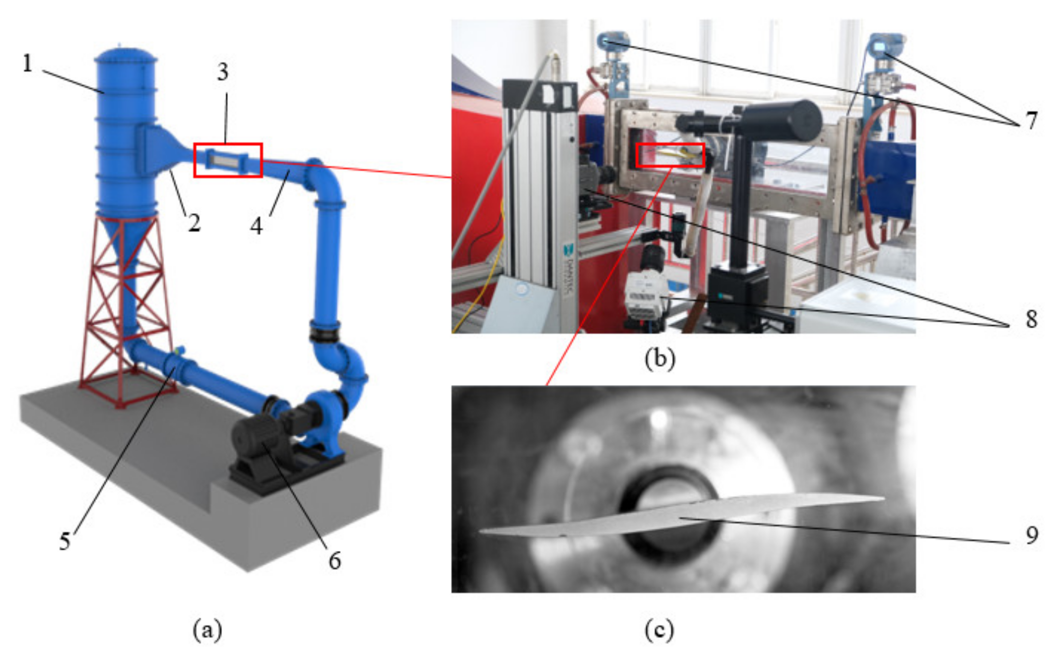
2. Experimental Equipment

The experimental conditions are provided by the cavitation tunnel stand of Yangzhou University. As shown in Figure 1a, the cyclic process of the cavitation tunnel is driven by a mixed-flow pump. First, the water flows out of the mixed-flow pump and enters the water tank through the pipe; then, the water flows through the guide vane in the water tank and sequentially passes through the shrink section, the test section, and the diffusion section; finally, it returns to the inlet of the mixed-flow pump. The water used in the experiment comes from city tap water. Before the experiment, the water was run at low pressure for one hour for degassing treatment. The size of the test section is 0.7 × 0.22 × 0.1 m³ (length × height × width), the stable flow velocity of the test section in the cavitation tunnel is 4–12 m/s, and the maximum inlet flow velocity can be up to 15 m/s. The inlet pressure is controlled by the water circulating vacuum pump connected to the inlet water tank, and the minimum inlet pressure can be reduced to 20 kPa. Figure 1b shows the cavitation around the hydrofoil captured by a high-speed camera with an acquisition frequency of 7500 f/s. The lift and drag data of the S-shaped hydrofoil are collected by six axis force and torque sensors. At the same time, the cavitation tunnel can also record the water temperature, inlet and outlet pressure, and flow. As shown in Figure 1c, the S-shaped hydrofoil with central of symmetry is used in this study. The chord length C and the span of the S-shaped hydrofoil are 150 mm and 100 mm. The maximum camber value of the S-shaped hydrofoil is 1.4% C, which is located at 23% C and 77% C. The angle of attack of the S-shaped hydrofoil is set to 6° in this study.

3. Numerical Setup and Validation

3.1. Governing Equation

As a multiphase flow problem, cavitation is usually simulated using the assumption of a homogeneous flow model. The basic equations for the homogeneous model are as follows:

Continuity and momentum equations:

$$\frac{\partial {\rho }_m}{\partial \mathrm{t}}+\frac{\partial \left({\rho }_m{u}_j\right)}{\partial x_j}=0$$

(1)

$$\frac{\partial \left({\rho }_m{u}_j\right)}{\partial \mathrm{t}}+\frac{\partial \left({\rho }_m{u}_i{u}_j\right)}{\partial x_j}=-\frac{\partial p}{\partial x_j}+\frac{\partial }{\partial x_j}\left[\left({\mu }_m+{\mu }_t\right)\left(\frac{\partial u_i}{\partial x_j}+\frac{\partial u_j}{\partial x_i}-\frac{2}{3}\frac{\partial u_k}{\partial x_k}{\delta }_{ij}\right)\right]$$

(2)

where $u_{i,j,k}$ are the velocity component and the subscripts i, j, k refer to the direction; ${\rho }_m$ and ${\mu }_m$ represent the mixture density and viscosity, and they are defined as follows:

$${\rho }_m={\rho }_v{\alpha }_v+{\rho }_l\left(1-{\alpha }_v\right)$$

(3)

$${\mu }_m={\mu }_v{\alpha }_v+{\mu }_l\left(1-{\alpha }_v\right)$$

(4)

where $\alpha$ represents the volume fraction, the subscripts l and v refer to the liquid and vapor phases.

3.2. Turbulence Model

The RNG k-ε model is used to close/solve the governing equation; ${\mu }_t$ is the turbulent viscosity of RNG k-ε turbulence model which is defined as:

$${\mu }_t=C_{\mu }\frac{k^2}{\epsilon }$$

(5)

where k and ε are the turbulence kinetic energy and the turbulence eddy dissipation are calculated by the transport equations of Equations (6) and (7).

$$\frac{\partial k}{\partial \mathrm{t}}+\frac{\partial u_{j}k}{\partial x_j}=P_t-\epsilon -\frac{\partial }{\partial x_j}\left[\left(v+\frac{v_t}{{\sigma }_k}\right)\frac{\partial k}{\partial x_j}\right]$$

(6)

$$\frac{\partial \epsilon }{\partial \mathrm{t}}+\frac{\partial u_j\epsilon }{\partial x_j}=C_{\epsilon 1}\frac{\epsilon }{k}{P}_t-C_{\epsilon 2}\frac{{\epsilon }^2}{k}+\frac{\partial }{\partial x_j}\left[\left(v+\frac{v_t}{{\sigma }_{\epsilon }}\right)\frac{\partial \epsilon }{\partial x_j}\right]$$

(7)

where P_t is the turbulent production term.

In order to simulate the unsteady cloud cavitation flow accurately, the FBM model proposed by Johansen [30] is used. The blending filter function f_FBM is used to modify the turbulent viscosity ${\mu }_t$ of RNG k-ε model. The eddy viscosity ${\mu }_t^{FBM}$ can be written as follows:

$${\mu }_t^{FBM}={\mu }_t{f}_{FBM}=C_{\mu }\frac{k^2}{\epsilon }\min \left(1,C_3\frac{\Delta \epsilon }{k^{\frac{3}{2}}}\right)$$

(8)

where C₃ = 1.0, $\Delta$ is the filter scale which is defined as: $\Delta ={\left(\Delta x·\Delta y·\Delta z\right)}^{1/3}$,$\Delta x$,$\Delta y$,$\Delta z$ are the grid length of three directions.

3.3. Cavitation Model

A cavitation model is used to describe the transformation between a liquid and its vapor, the Zwart–Gerber–Belamri (ZGB) has been chosen in our study. The ZGB cavitation model is based on the Rayleigh–Plesset equation, which is defined as:

$$\frac{\partial ({\rho }_v{\alpha }_v)}{\partial \mathrm{t}}+\frac{\partial ({\rho }_v{\alpha }_v{u}_j)}{\partial x_j}={\dot{m}}^{+}-{\dot{m}}^{-}$$

(9)

where ${\dot{m}}^{+}$ and ${\dot{m}}^{-}$ represent the evaporation and the condensation source terms, which are presented in Equation (10).

$$\left.\begin{array}{c}{\dot{m}}^{+}=F_{evap}\frac{3{\rho }_v{r}_{nuc}\left(1-{\alpha }_v\right)}{R_b}\sqrt{\frac{2}{3}\frac{\left(p_v-p\right)}{{\rho }_l}} if p<p_v\\ {\dot{m}}^{-}=F_{cond}\frac{3{\rho }_v{\alpha }_v}{R_b}\sqrt{\frac{2}{3}\frac{\left(p-p_v\right)}{{\rho }_l}} if p>p_v\end{array}\right\}$$

(10)

where $r_{nuc}$ represents the volume fraction of nucleation in water and with the value of 5 × 10⁻⁴, $R_b$ is the radius of the bubble size with the value of 10⁻⁶ m, $F_{evap},$ and $F_{cond}$ represent coefficients for the processes of evaporation and condensation with the recommended values of 50 and 0.01. $p_v$ is the saturated vapor pressure which is determined as 5033.5 Pa by the local temperature measured by the temperature sensor. Considering the influence of the turbulent during the numerical simulation of cavitation flow, the $p_{turb}$ is introduced to modify $p_v$, and the $p_v^{\prime }$ is defined as follows:

$$p_v^{\prime }=p_v+\frac{p_{turb}}{2}$$

(11)

$$p_{turb}=0.39{\rho }_{m}k$$

(12)

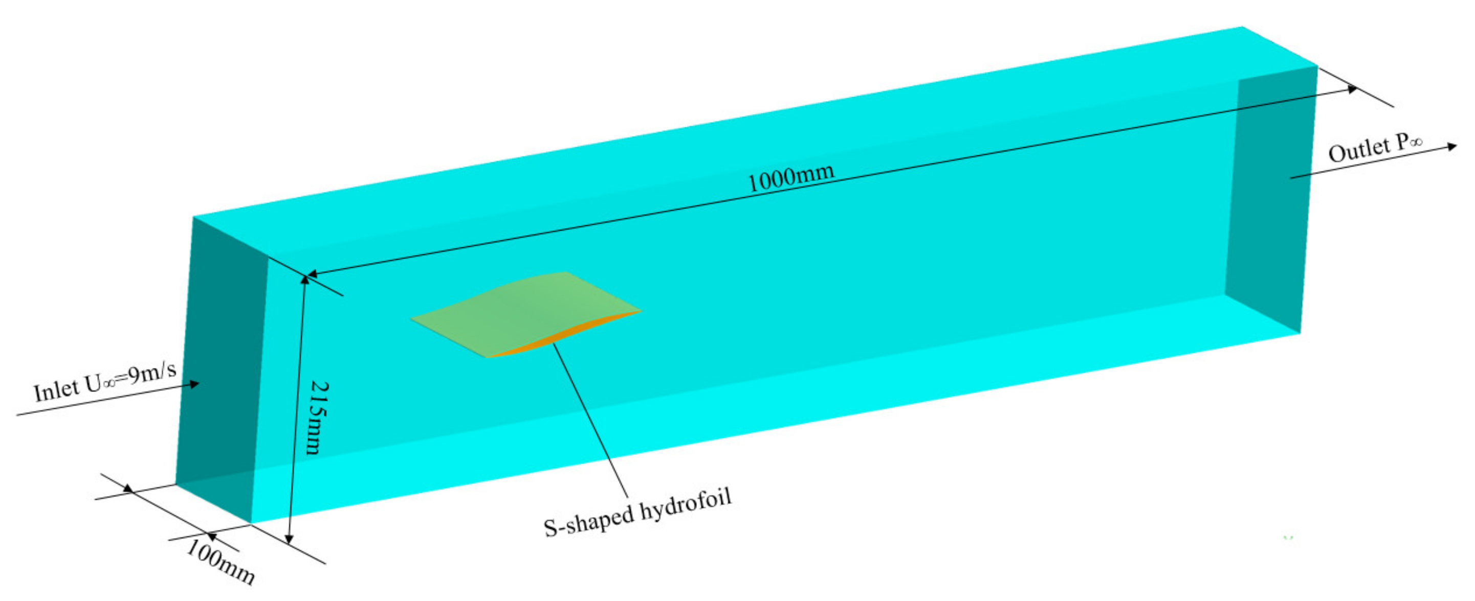
3.4. Numerical Setup and Mesh Validation

Figure 2 shows a computational domain consistent with the experimental test section. The velocity at the inlet is U_∞ = 9 m/s, and the static pressure at the outlet is used to adjust the cavitation number $\sigma =\left(P_{in}-P_V\right)/0.5\rho U_{\infty }^2$ to be consistent with the experiments. In order to ensure that the value of y+ on the hydrofoil surface is within 1, the height of the first layer near the wall of the mesh around the hydrofoil is calculated as $2.67\times {10}^{-6} \mathrm{m}$, according to the inlet Reynolds number $Re=\rho U_{\infty }l/\mu =1.35\times {10}^6$. In order to ensure that the unsteady numerical calculation can capture the details of cloud cavitation evolution, the time interval is 1/100 times of the time of cloud cavitation period collected from the experiment. As shown in

Table 1. Mesh verification for S-shaped hydrofoil ($\mathsf{\sigma }=0.98$, α = 6°).

	CL	CD	St	Nodes
Mesh1	0.665	0.073	0.56	5388416
Mesh2	0.670	0.077	0.60	6386688
Mesh3	0.673	0.078	0.61	7432148
Exp	0.691	0.083	0.64

, by arranging different numbers of nodes in the span of the S-shaped hydrofoil, three grid schemes are divided into numerical calculations and the lift coefficient C_L, drag coefficient C_D, and Strouhal number St (St = fl/U_∞) of the three grid schemes are compared with the data collected in the experiment. As shown in Figure 3a, the mesh was chosen as the final solution and Figure 3b is the y+ distribution on the surface of the hydrofoil.

4. Discussion

4.1. Different Cavitation Behaviors of S-Shaped Hydrofoil

The different cavitation behaviors at different cavitation numbers were recorded using HSC on the side of the test section. According to the HSVs (high speed videos), the maximum length of the cavity around the S-shaped hydrofoil increased with a decrease in the cavitation number, and the cavitation behaviors gradually changed from “stable” sheet cavity to periodic cloud cavity in Figure 4. When σ = 1.73, there was only a small amount of stable attached bubble at the leading edge of the S-shaped hydrofoil. When the cavitation number changed to 1.23, the maximum cavity length reached l/C = 0.25, and a small amount of periodic U-shaped shedding structure was observed at the tail of the attached cavity. When the inlet pressure decreased, the cavitation number changed from 1.23 to 0.98 and the maximum length of the cavity gradually increased to l/C = 0.50. The “stable” sheet cavitation transformed into an unstable periodic cloud cavitation and the cloud cavitation shedding cycle time was approximately T_cycle = 26 ms. As the cavitation number was reduced to 0.49, the maximum cavity length grew from l/C = 0.50 to l/C = 1. The shedding time of cloud cavitation gradually increased, and the cycle time T = 6 Tcycle was at σ = 0.49. In the process of decreasing the cavitation number, the maximum cavity length was linearly related to the cavitation number, and the slope was approximately −0.41. After cloud cavitation occurred, the maximum cavity length was still linearly related to the cavitation number, but the slope was approximately −1.01. It was observed that at the maximum cavity length of l/C > 0.25, the cavity evolved from a stable attachment to cloud shedding, and the growth rate of the maximum cavity length gradually became faster.

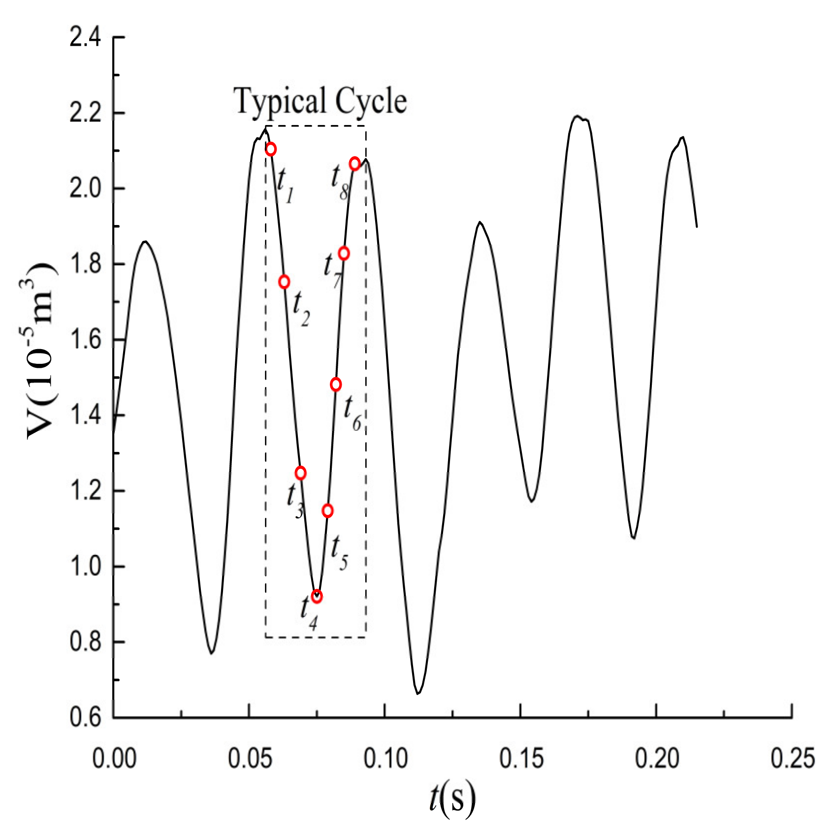
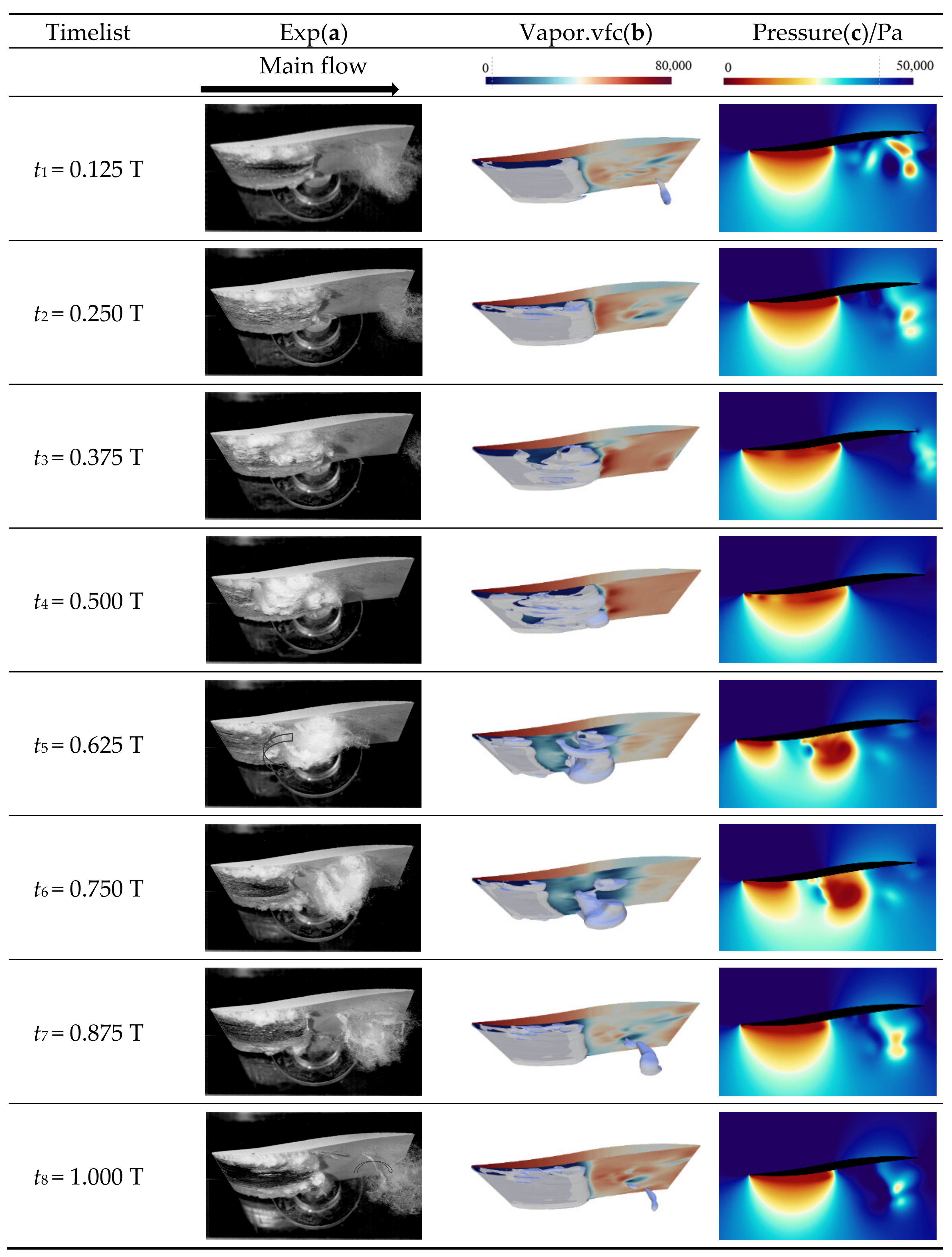
4.2. The Periodic Behavior of Cloud Cavitation

For the purpose of the dynamic characteristics of cloud cavity around the S-shaped hydrofoil when cloud cavitation occurs, an obviously periodic cloud cavitation condition σ = 0.98 was selected for analysis. Figure 5 shows the numerical results of the evolution of the cavity volume in this working condition. It can be clearly seen that the volume of cavitation changes constantly and it has obvious periodicity—the average frequency of shedding f = 1/T_cycle = 35.7 Hz—which agrees well with the test results (38.4 Hz). To study the unsteady flow during the periodic change of cloud cavitation, a typical cycle (from t₁ to t₈) was selected from Figure 5 for analysis. The cavity volume is defined as follows:

$$Vcav={\displaystyle \sum }_{i=1}^n{\alpha }_i{v}_i$$

(13)

Figure 6 shows the change of cloud cavitation from t₁ to t₈ (Figure 5) when the cavitation number is 0.98. Figure 6a shows the result of high-speed visualization in the experiment. In Figure 6a, the cavity experienced one typical periodic process of cloud cavitation: growth-shedding-collapse (re-growth) and the cycle time T_cycle = 26 ms. During t₁ to t₂, the cavity length is maintained at the maximum value of l/C = 0.5, but the interface between vapor and liquid has gradually become blurred due to the joint work of the re-entrant jets and the side-entrant jets near the hydrofoil surface, and the cavity immediately changes from “stable” sheet cavitation to shedding. From t₃ to t₆, the re-entrant jets cut off the sheet cavity, but the remaining sheet cavity continued to grow, while the shed cavity rapidly transformed into cloud cavitation. In the process of the cavity moving to the tail of the S-shaped hydrofoil, the cloud cavitation was rolled up irregularly by the combined action of the re-entrant jets and the side-entrant jets. The cloud cavity gradually collapsed, and the length of the sheet cavity reached its maximum again during the time from t₇ to t₈. The liquid–vapor interface of the re-grown sheet cavity reverts to smooth and stable, but the two sides of the sheet cavity are turbulent due to the influence of side walls.

The cavity in a numerical simulation, which is displayed by the iso-surfaces of the vapor volume fraction with α_v = 0.1, is shown in Figure 6b and the suction and pressure surface of the S-shaped hydrofoil is colored by the value of pressure. Figure 6c shows the pressure distribution in the mid-plane of the S-shaped hydrofoil. The numerical results of the sheet cavitation shedding process are basically consistent with the experiment as shown in Figure 6b. Before the shedding of the sheet cavitation, the low-pressure area on the hydrofoil surface is mainly distributed in the sheet cavity coverage area, and there is also the influence of cloud cavitation in the back half of the S-shaped hydrofoil in the last cycle. When the re-entrant jet moves to a position of approximately l/C = 0.2 to cut off the sheet cavity on the suction surface of the hydrofoil, the distribution of the low pressure on the hydrofoil suction surface first breaks and then moves towards the trailing edge of the hydrofoil with the large-scale cloud cavity. The results show that everything collapses when the position of the cloud cavitation moves to l/C = 0.75, which is close to the experimental observation. The suction surface pressure distribution of the hydrofoil at t = t₈ is basically the same as t = t₁. The front half of the hydrofoil is covered by sheet cavity, and the area of lower pressure is also distributed on the suction surface. With the disappearance of the cloud cavity, the effect of cavitation on the surface pressure of the back half of the hydrofoil gradually disappears. The shedding and regeneration process of the sheet cavity and the movement of the cloud cavity are the main factors that cause the pressure change at the mid-plane in Figure 6c, and the low-pressure area of the mid-plane is mainly concentrated in the area covered by the sheet cavity and around the cavitation of large-scale cloud cavity. Even if the cloud cavitation is completely dispersed (t = t₂), the influence of the flow field will still exist (t = t₃). The hydrofoil surface pressure between the sheet cavity and the large-scale cloud cavity is increased by the pressure of the water flow (t = t₅, t = t₆). With the re-growth of the sheet cavity and the dissipation of the large-scale cloud cavity, the low-pressure area in the middle section of the hydrofoil re-gathers into the sheet cavity coverage area (t = t₇, t = t₈).

As shown in Figure 7, t = t₃, t₅, t₈ are the moments before the shedding of the cloud cavity, the complete shedding and dissipation of the cloud cavity. Based on the observed results of HSVs, it can be found that re-entrant jets are always present in the tail of a cloud cavity. The interface between vapor and liquid still exists, but the inside of the sheet cavity has been filled by the re-entrant jets at t = t₃. As t = t₅, the fractured sheet cavity continues to develop, while the cloud cavity causes a significant rotating velocity vector around the hydrofoil when moving toward the tail of the S-shaped hydrofoil, which easily induces the generation of vortices in the flow field around the hydrofoil. The cavity length grows again to the maximum cavity length of l/C = 0.5 under this working condition. The adverse pressure gradient at the tail of the sheet cavity closed zone again forms re-entrant jets that can cut off the stable cavity and the cavity will enter next shedding process.

4.3. Cavitation-Vortex Interactions

The re-entrant jets caused by the gradient of pressure and the movement of the shedding cavity can easily cause high shear flow around the hydrofoil and further induce a complex vortex structure. The Q-criterion [31] (Hunt et al., 1988) can better describe the details of the vortex caused by cavitation, which is defined as:

$$Q=\frac{1}{2}\left({\Vert \Omega \Vert }^2-{\Vert S\Vert }^2\right)$$

(14)

where Ω and S represent the vorticity tensor and the strain rate tensor, respectively.

The iso-surface of Q-criterion with the value of 2 × 10⁵ s⁻² is displayed in Figure 8, and it is colored with turbulent kinetic energy. In Figure 8, the vortex identified by the Q-criterion are mainly concentrated around the sheet and the cloud cavity. The re-entrant jets caused by the adverse pressure gradient and the motion of the cloud cavity can easily cause high shear flow around the hydrofoil and further induce complex vortex structures. The vortex structure generated around the cloud cavity is described by the Q-criterion, and the turbulent kinetic energy is used for coloring. Figure 8 shows the vortex identified by the Q-criterion is concentrated in the sheet cavity attached to the suction surface and around the cloud cavity. As the cloud cavitation moves to the trailing edge, the vortex around the cloud cavity changes complexly. The rotation and dissipation of the cloud cavity causes the vortex structure to gradually present a U-shape. When the cloud cavity leaves the hydrofoil surface, the vortex structure quickly disappears. At the position where the sheet cavitation is cut off by re-entrant jets, the intersection of re-entrant jets and the main flow results in the highest turbulent kinetic energy in the whole cycle.

The shedding process of sheet cavitation induces complex vortex structures around the hydrofoil. In order to characterize the interaction between the cloud cavitation and the vortex, a vorticity transport equation was introduced to study the composition of vorticity.

$$\frac{D\mathit{\omega }}{Dt}=\left(\mathit{\omega }·\nabla \right)\mathit{V}-\mathit{\omega }\left(\nabla ·\mathit{V}\right)+\frac{\nabla {\rho }_m\times \nabla \rho }{{\rho }_m^2}+\left(v_m+v_t\right){\nabla }^2\mathit{\omega }$$

(15)

One the left side, the term of the equation is the rate of change of vorticity over time. On the right side, the first segment is the vortex stretching, which represents the stretching of the vorticity caused by the velocity gradient. The second segment is the vortex dilatation, which represents the stretching of the vorticity caused by the change in expansion and the contraction of the vapor volume in the cavitating flow. The third term on the right is the baroclinic term, which is caused by the density and the pressure gradient between the vapor and the liquid in the cavitating flow. The fourth term on the right is a viscous diffusion term, which can be ignored in a high Reynolds number.

In Figure 9, from left to right are the vapor volume fraction, vorticity, vortex stretching, dilatation, and baroclinic terms at the mid-plane. It can be seen from Figure 9 that the vorticity is mainly concentrated in the sheet cavitation and the cloud cavitation. The periodic process of cloud cavitation causes a periodic change in the vorticity around the S-shaped hydrofoil. The vorticity at the sheet cavity is stably concentrated in the cavity, while the vorticity caused by the movement of the shedding cloud is the maximum at the beginning of the shedding, and it decreases continuously as the cloud cavitation moves toward the tail of the S-shaped hydrofoil. It is worth noting that the vorticity caused by the shedding cloud does not disappear immediately with the disappearance of shedding cloud; it does not disappear into the main flow until it leaves the trailing edge of the hydrofoil. Among them, the vortex stretching term is much larger than the vortex dilatation and the baroclinic terms, and it is the main component of the vorticity energy. The vortex dilatation and the baroclinic terms are mainly concentrated in the inside and at the boundary of the cavity region, which provides the vorticity changes in the inside and the boundary of the cavity, and their magnitude disappears immediately with the collapse of the cavitation.

4.4. The Lift and Drag Characteristics Affected by Cavitation

Due to the unique shape of the S-shaped hydrofoil, the lift–drag characteristics and the surface pressure distribution of the S-shaped hydrofoil are significantly different from those of other hydrofoils commonly used in hydraulic machinery. Figure 10 shows the lift generated by the S-shaped hydrofoil. Moreover, the periodic evolution of cloud cavity causes periodic changes in the pressure around the S-shaped hydrofoil in Figure 6, and it will further affect the change of the lift and drag of the hydrofoil. Figure 11a,b shows the evolution of the lift and drag of the hydrofoil when the cavitation number is 0.98 and the angle of attack is 6°. Figure 11c,d are the changes in the surface pressure distribution at the intersection line of the mid-plane and the hydrofoil surface at different cavitation numbers and at different moments. In order to compare the pressure characteristics under different cavitation numbers at the same order of magnitude, the pressure coefficient $Cp$ is used to dimensionless pressure data.

$$Cp=\frac{p-\overline{p}}{0.5\rho u^2}$$

(16)

where $p$ is the pressure on the surface of the hydrofoil, and $\overline{p}$ is the average pressure of hydrofoil.

Figure 11a,b reflect that the lift and drag of the hydrofoil have undergone two periodic changes in one cloud cavitation cycle, and the evolution trend of lift and drag is basically the same. The first peak of lift and drag is between t = t₂ and t = t₃, mainly caused by the influence of the shedding cloud cavity from the last period. The second lift and drag peak at the instant t = t₆ is different from the lift–drag characteristics of other hydrofoils under the cloud cavitation condition, which can be explained as the cloud cavity moves to the back half of the hydrofoils, resulting in a decrease in the reverse lift and thus increasing the total lift.

In Figure 11c, when the cavitation number has decreased to 1.73, no cavitation occurs at the leading edge of the S-shaped hydrofoil, and the surface pressure coefficient of the suction surface and the pressure surface of the hydrofoil is equal at approximately 0.6C, forming an intersection point in the pressure data. Before 0.6C, the pressure distribution on the suction side of the S-shaped hydrofoil was lower than that on the pressure side, but after 0.6C, the pressure distribution on the suction side was higher than that on the pressure side. According to the pressure distribution characteristics of the hydrofoil, it can be generally considered that the S-shaped hydrofoil generates the lift required by the hydraulic machinery design in the front half; while, the lift generated by the back half of the hydrofoil is in the opposite direction to that of the front half, as is shown in Figure 10. As a result, the lift of the S-shaped hydrofoil is usually lower than the common hydrofoil used in hydraulic machinery with similar geometrical parameters. In practical application, the S-shaped hydrofoil needs to increase the angle of attack to meet the needs of lift applications. When σ decreases from 1.48 to 0.98, the maximum cavity length on the hydrofoil increases gradually, but the maximum cavity length has not reached 0.6C. The low-pressure area continues to grow, but the position of the pressure intersection of the hydrofoil is almost unaffected by the cavity and it is still at 0.6C. When σ is further reduced to 0.73, the maximum cavity length has reached 0.8. The position of the pressure intersection of the time-average pressure coefficient of the hydrofoil is affected by the average cavity length and it is delayed to the position of 0.9C. Under different cavitation numbers, when the average length of the cavity is less than 0.6C, there is a low-pressure area positively related to the cavity length at the leading edge of the suction surface of the hydrofoil due to the influence of the sheet cavity, and the position where the pressure value of the suction surface and the pressure surface of the airfoil is equal remains unchanged at 0.6C. When the time-average cavity length is greater than 0.6C, the low-pressure area of the suction surface of the hydrofoil affected by the cavity has reached 0.6C, and the position of the pressure intersection is also delayed to the position behind the cavity. Figure 11c reflects the relative stability of the sheet cavitation effect on the pressure distribution of the hydrofoil, but for the cloud cavity where the cavity length changes periodically, it cannot fully demonstrate the periodic characteristics of the pressure distribution; therefore, in Figure 11d, the surface pressure coefficient distribution of the hydrofoil from t₁ to t₈ of a typical cloud cavity period is taken for analysis.

In Figure 11d, the pressure coefficient of the pressure surface is basically unchanged, and the pressure coefficient of the suction surface is significantly different at different times due to the influence of the cloud cavity, resulting in a change in the position of the pressure intersection between 0.5 and 0.8. As t = t₁ − t₄ or t₇ − t₈, the pressure coefficient of the front half of the hydrofoil is relatively close, and the pressure intersection points are all within the position of 0.5 to 0.6. However, at the instant t = t₂, the pressure coefficient values of the suction surface and the pressure surface intersect for the second time at the position of 0.8C due to the influence of the shedding cloud cavity from the last period, and the positive lift is again generated from 0.8C to 1.0C. The increase in the positive lift and the decrease in the reverse lift are the main reasons for the first peak of the lift coefficient. At the instant t = t₅, the pressure coefficient on the suction surface rises from 0.2C to 0.3C, mainly because the cloud cavity has just shed, the space between the sheet cavity and the shedding cloud cavity is filled by the main flow. From 0.3C to 0.5C, the pressure coefficient on the suction surface of the hydrofoil decreased due to the large cloud cavity affecting the pressure coefficient distribution on the suction surface, and then the pressure coefficient increased again at 0.65C to 0.7C and crossed with the pressure coefficient on the pressure surface. At the instant t = t₆, the back half of the suction surface is affected by the shedding cloud cavity and the pressure intersection position between the suction surface and the pressure surface moves backward, the pressure difference between the suction surface and the pressure surface is very small, resulting in a reverse lift that reaches the minimum value and the total lift and drag coefficient reaches the peak for the second time in one typical cycle.

5. Conclusions

The experiment was conducted to study the flow structures of cloud cavitation around an S-shaped hydrofoil. The unsteady evolution of the vortex, pressure distribution and lift–drag caused by the cloud cavitation are further studied with numerical simulation. The work can be summarized as follows:

(1)

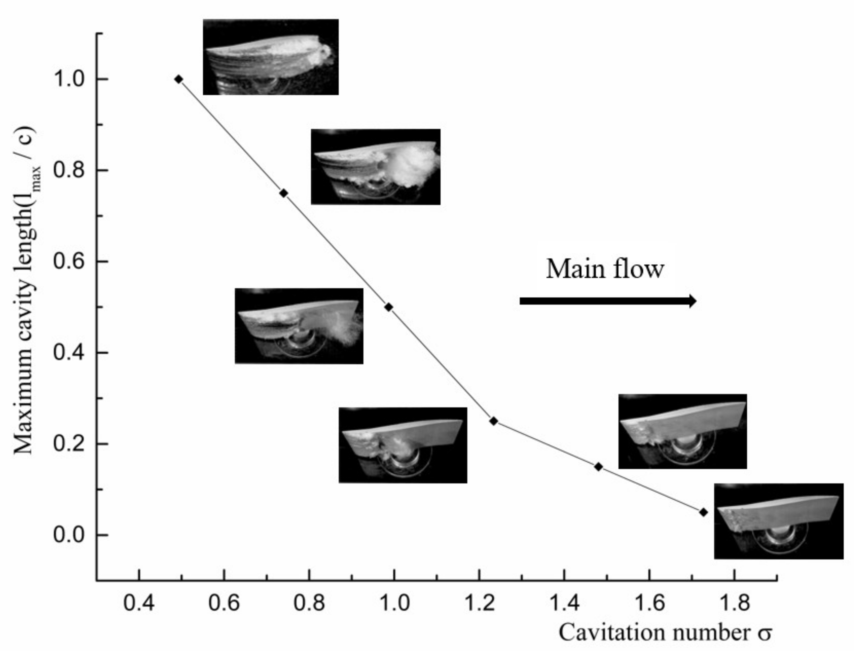
At α = 6°, the maximum cavity length of the hydrofoil increases linearly with a decrease in the cavitation number; but, after cloud cavitation occurs, the growth rate of the maximum cavity length of the cloud cavitation is faster than that of the sheet cavitation. This means that the occurrence of cloud cavitation provides favorable conditions for the next cycle of sheet cavity growth.

(2)

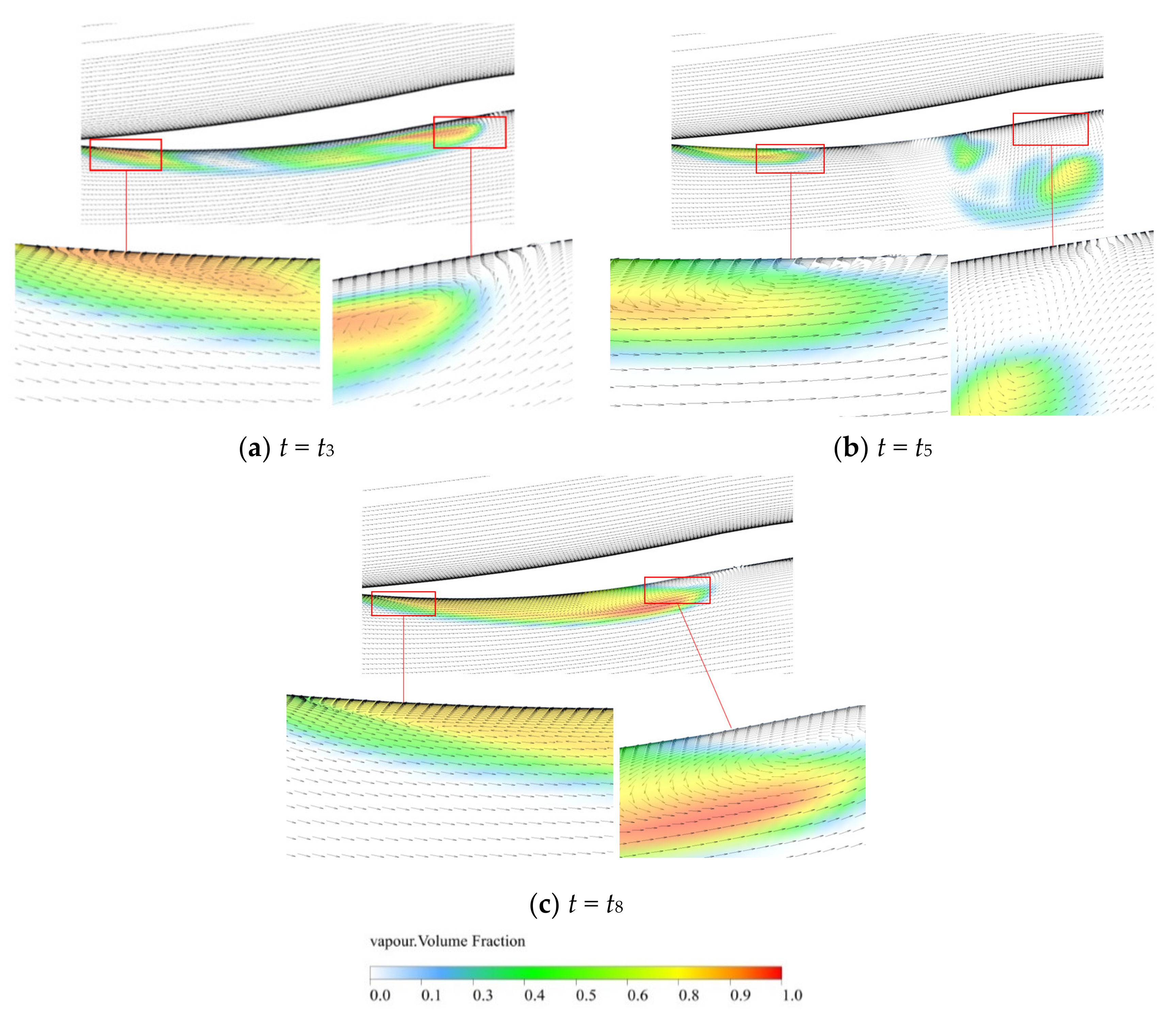
The cloud cavitation process calculated by numerical simulation shows the same trend as the experiment. The FBM turbulence model and the ZGB cavitation model can better simulate the cavitating flow around the S-shaped hydrofoil and successfully reproduce the growth of sheet cavity and the shedding process of cloud cavity. The numerical results show that the re-entrant jet always exists in the tail of the cavity. The re-entrant jets reach the maximum intensity and cut off the cavity successfully when the maximum cavity length is reached.

(3)

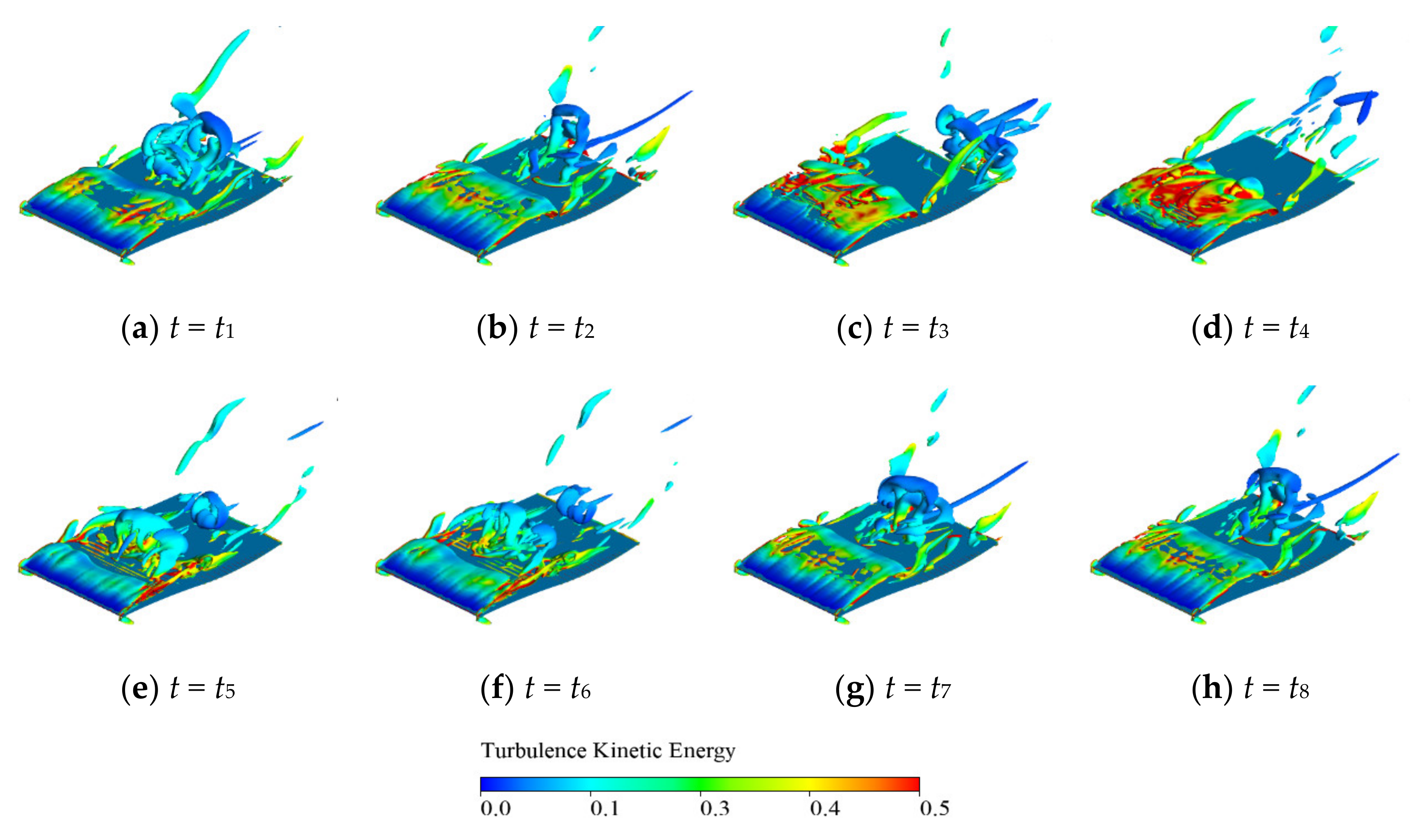
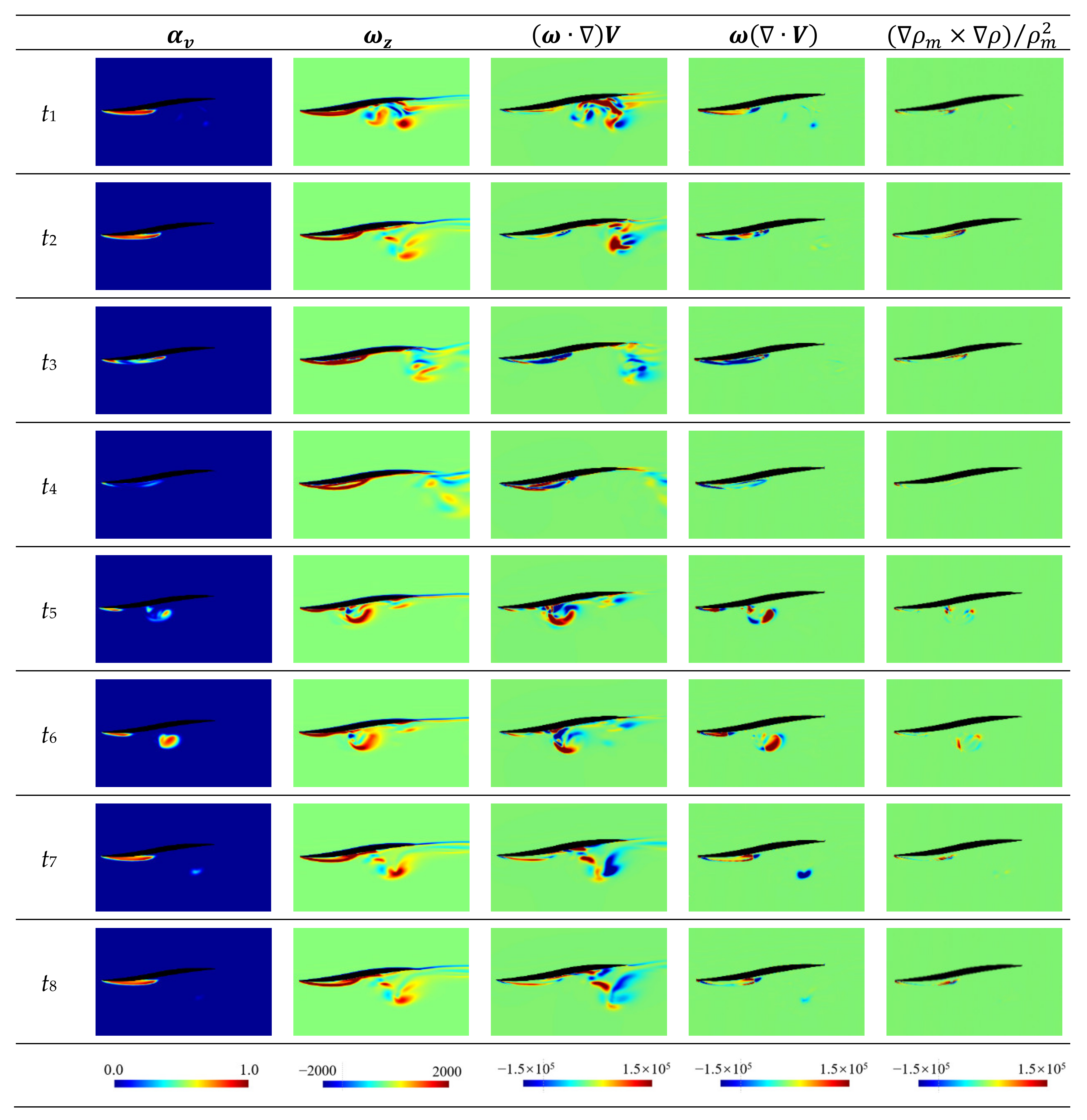
The vortex structures around the cavitation are described using the Q-criterion. The shedding of sheet cavity plays an important role in the complex vortex structure around the S-shaped hydrofoil. The vortex is mainly concentrated around the cloud cavitation, and the shape of the vortex gradually presents a U-shaped structure as the cloud cavitation dissipates. According to the vorticity transport equation, it turns out that the vortex stretching term is the main source of vorticity generated in the process of cloud cavitation.

(4)

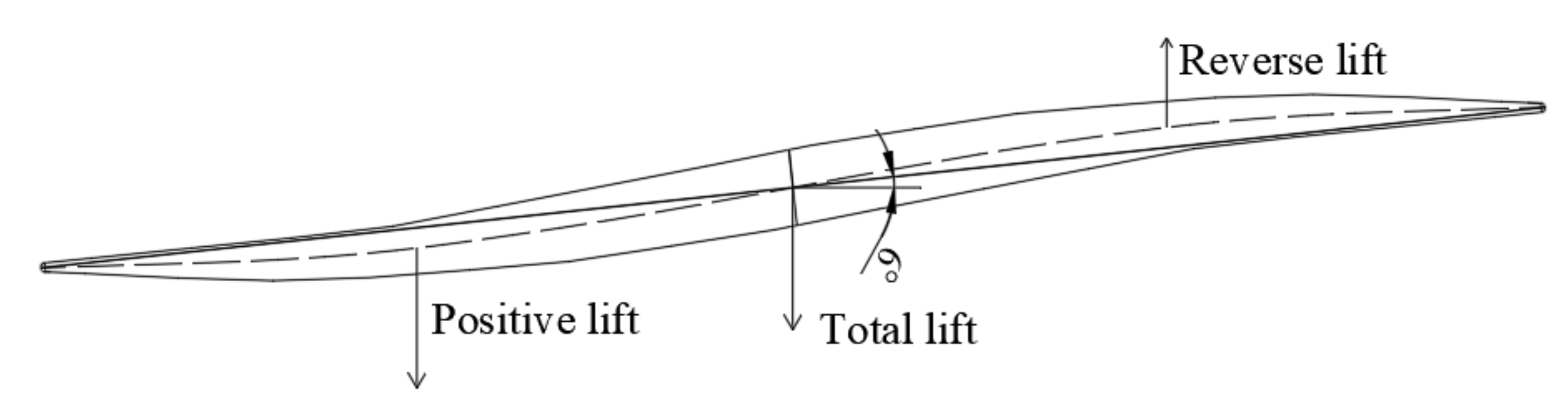
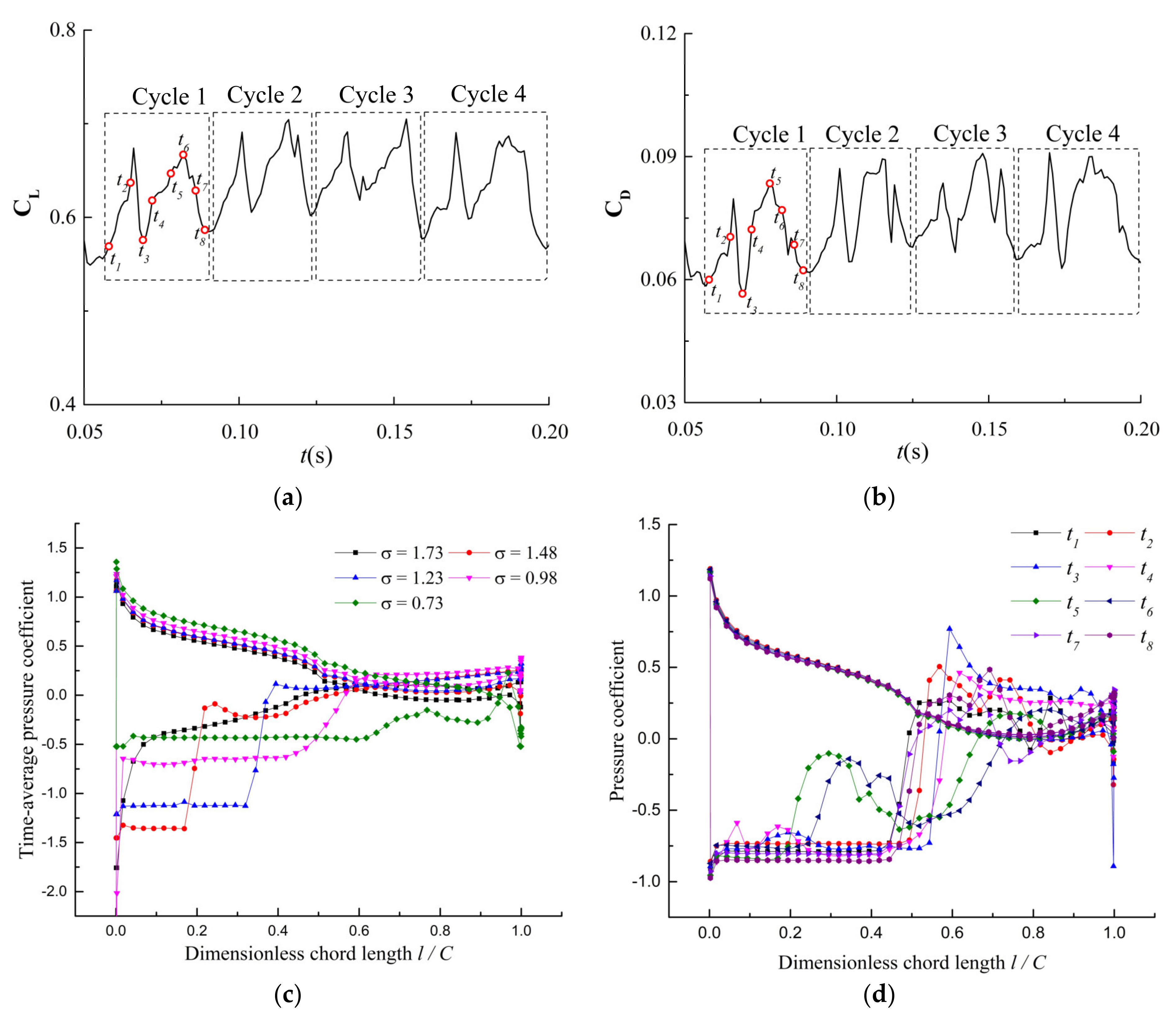
Under a cavitation-free condition, the unique shape of the S-shaped hydrofoil causes the time-average pressure coefficient of the suction surface and the pressure surface to be equal at l/C = 0.6. Before l/C = 0.6, the pressure coefficient value of the suction surface is lower than the pressure surface, and the hydrofoil produces positive lift. After l/C = 0.6, the time-average pressure coefficient value of the pressure surface is lower than the suction surface, and the hydrofoil produces a reverse lift, resulting in an overall lift of the S-shaped hydrofoil that is lower than other hydrofoils. As the cavity length is less than 0.6C, the cavity has almost no effect on the position of the intersection of the time-averaged pressure. As the cavity length is greater than 0.6C, the cavity will push the intersection of the time-averaged pressure to the back of the cavity. An unusual phenomenon is observed in that the lift–drag coefficient experienced two obvious peaks in one typical cycle of cloud cavitation. The first peak is due to the influence of the cloud cavitation from the previous period on the pressure coefficient of the suction surface, which leads to an increase in the forward lift and a decrease in the reverse lift, thus the total lift and drag coefficient reaches a peak. The second peak is due to the motion of the shedding cloud, which caused the reverse lift to reach the lowest value in one typical cycle of cloud cavitation, and the total lift and drag coefficient reached the peak again.

References

1. Brennen, C.E. Cavitation and Bubble Dynamics; Oxford University Press: New York, NY, USA, 1995. [Google Scholar]
2. Franc, J.P.; Michel, J.M. Fundamentals of Cavitation; Springer: Dordrecht, The Netherlands, 2005. [Google Scholar] [CrossRef] [Green Version]
3. Dular, M.; Bachert, R.; Stoffel, B.; Širok, B. Experimental evaluation of numerical simulation of cavitating flow around hydrofoil. Eur. J. Mech. B-Fluid 2004, 24, 522–538. [Google Scholar] [CrossRef]
4. Luo, X.W.; Ji, B.; Tsujimoto, Y. A review of cavitation in hydraulic machinery. J. Hydrodyn. 2016, 28, 335–358. [Google Scholar] [CrossRef]
5. Knapp, R.T. Recent Investigations of the Mechanics of Cavitation and Cavitation Damage. J. Fluids Eng.-Trans. ASME 1955, 77, 1045–1054. [Google Scholar]
6. Kubota, A.; Kato, H.; Yamaguchi, H.; Maeda, M. Unsteady Structure Measurement of Cloud Cavitation on a Foil Section Using Conditional Sampling Technique. J. Fluids Eng. 1989, 111, 204–210. [Google Scholar] [CrossRef]
7. Kawanami, Y.; Kato, H.; Yamaguchi, H.; Tanimura, M.; Tagaya, Y. Mechanism and Control of Cloud Cavitation. J. Fluids Eng. 1997, 119, 788–794. [Google Scholar] [CrossRef]
8. Wang, G.; Senocak, I.; Shyy, W.; Ikohagi, T.; Cao, S. Dynamics of attached turbulent cavitating flows. Prog. Aerosp. Sci. 2001, 37, 551–581. [Google Scholar] [CrossRef]
9. Foeth, E.J.; van Doorne, C.W.H.; van Terwisga, T.; Wieneke, B. Time resolved PIV and flow visualization of 3D sheet cavitation. Exp. Fluids 2006, 40, 503–513. [Google Scholar] [CrossRef]
10. Foeth, E.J.; van Terwisga, T.; van Doorne, C. On the collapse structure of an attached cavity on a three-dimensional hydrofoil. J. Fluids Eng.-Trans. ASME 2008, 130, 71303. [Google Scholar] [CrossRef] [Green Version]
11. Seyfi, S.; Nouri, N.M. Experimental studies of hysteresis behavior of partial cavitation around NACA0015 hydrofoil. Ocean Eng. 2020, 217, 107482. [Google Scholar] [CrossRef]
12. Morgut, M.; Nobile, E.; Biluš, I. Comparison of mass transfer models for the numerical prediction of sheet cavitation around a hydrofoil. Int. J. Multiph. Flow 2011, 37, 620–626. [Google Scholar] [CrossRef]
13. Kunz, R.F.; Boger, D.A.; Stinebring, D.R.; Chyczewski, T.S.; Lindau, J.W.; Gibeling, H.J.; Venkateswaran, S.; Govindan, T.R. A preconditioned Navier–Stokes method for two-phase flows with application to cavitation prediction. Comput. Fluids 2000, 29, 849–875. [Google Scholar] [CrossRef]
14. Singhal, A.K.; Athavale, M.M.; Li, H.; Jiang, Y. Mathematical Basis and Validation of the Full Cavitation Model. J. Fluids Eng. 2002, 124, 617–624. [Google Scholar] [CrossRef]
15. Zwart, P.J.; Gerber, A.G.; Belamri, T. A two-phase flow model for predicting cavitation dynamics. In Proceedings of the International Conference on Multiphase Flow, Yokohama, Japan, 30 May–4 June 2004. [Google Scholar]
16. Ji, B.; Luo, X.W.; Wu, Y.L.; Peng, X.X.; Duan, Y.L. Numerical analysis of unsteady cavitating turbulent flow and shed-ding horse-shoe vortex structure around a twisted hydrofoil. Int. J. Multiph. Flow 2013, 51, 33–43. [Google Scholar] [CrossRef] [Green Version]
17. Huang, B.; Wang, G.Y.; Zhao, Y. Numerical simulation unsteady cloud cavitating flow with a filter-based density correction model. J. Hydrodyn. 2014, 26, 26–36. [Google Scholar] [CrossRef]
18. Wang, Z.; Li, L.; Cheng, H.; Ji, B. Numerical investigation of unsteady cloud cavitating flow around the Clark-Y hydrofoil with adaptive mesh refinement using Open FOAM. Ocean Eng. 2020, 206, 107349. [Google Scholar] [CrossRef]
19. Ji, B.; Luo, X.; Arndt, R.E.; Wu, Y. Numerical simulation of three dimensional cavitation shedding dynamics with special emphasis on cavitation–vortex interaction. Ocean Eng. 2014, 87, 64–77. [Google Scholar] [CrossRef]
20. Huang, B.; Zhao, Y.; Wang, G. Large Eddy Simulation of turbulent vortex-cavitation interactions in transient sheet/cloud cavitating flows. Comput. Fluids 2014, 92, 113–124. [Google Scholar] [CrossRef]
21. Zhang, M.; Chen, H.; Wu, Q.; Li, X.; Xiang, L.; Wang, G. Experimental and numerical investigation of cavitating vortical patterns around a Tulin hydrofoil. Ocean Eng. 2019, 173, 298–307. [Google Scholar] [CrossRef]
22. Yan, H.; Zhang, H.Z.; Zeng, Y.S.; Wang, F.; He, X.Y. Lift-drag characteristics and unsteady cavitating flow of bionic hydrofoil. Ocean Eng. 2021, 225, 108821. [Google Scholar] [CrossRef]
23. Pendar, M.R.; Esmaeilifar, E.; Roohi, E. LES Study of Unsteady Cavitation Characteristics of a 3-D Hydrofoil with Wavy Leading Edge. Int. J. Multiph. Flow 2020, 132, 103415. [Google Scholar] [CrossRef]
24. Movahedian, A.; Pasandidehfard, M.; Roohi, E. LES investigation of sheet-cloud cavitation around a 3-D twisted wing with a NACA 16012 hydrofoil. Ocean. Eng. 2019, 192, 106547. [Google Scholar] [CrossRef]
25. Živan, S.; Miloš, J.; Jasmina, B.J. Design and performance of low-pressure reversible axial fan with doubly curved pro-files of blades. J. Mech. Sci. Technol. 2018, 32, 3707–3712. [Google Scholar]
26. Ma, P.F.; Wang, J.; Wang, H.F. Investigation of performances and flow characteristics of two bi-directional pumps with different airfoil blades. Sci. China Technol. Sci. 2018, 61, 1588–1599. [Google Scholar] [CrossRef]
27. Li, D.Y.; Wang, H.J.; Qin, Y.L.; Han, L.; Wei, X.Z.; Qin, D.Q. Entropy production analysis of hysteresis characteristic of a pump-turbine model. Energy Convers. Manag. 2017, 149, 175–191. [Google Scholar] [CrossRef]
28. Ramachandran, R.; Krishna, H.; Narayana, P. Cascade experiments over “S” blade profiles. J. Energy Eng. 1986, 112, 37–50. [Google Scholar] [CrossRef]
29. Chacko, B.; Balabaskaran, V.; Tulapurkara, E.G.; Krishna, H.C.R. Performance of S-Cambered Profiles with Cut-Off Trailing Edges. J. Fluids Eng. 1994, 116, 522–527. [Google Scholar] [CrossRef]
30. Johansen, S.T.; Wu, J.; Shyy, W. Filter-based unsteady RANS computations. Int. J. Heat Fluid Flow 2004, 25, 10–21. [Google Scholar] [CrossRef]
31. Hunt, J.C.R.; Wray, A.A.; Moin, P. Eddies, streams, and convergence zones in turbulent flows. In Proceedings of the 1988 Summer Program in its Studying Turbulence Using Numerical Simulation Databases, 2; (SEE N89–24538 18–34); Center for Turbulence Research: Stanford, CA, USA, 1988. [Google Scholar]
Figure 1. (a) Sketch of the cavitation water tunnel (b) image of test section (c) the S-shaped hydrofoil. 1. Water tank 2. Shrink Section 3. Test Section 4. Diffusion Section 5. Electromagnetic flowmeter 6. Pump 7. Pressure sensor 8. High-speed camera 9. S-shaped hydrofoil.
Jmse 10 00386 g001
Figure 2. Computational domain of the S-shaped hydrofoil.
Jmse 10 00386 g002
Figure 3. The computational mesh and the y+ distribution around the S-shaped hydrofoil. (a) Mesh2 (L.E is the Leading Edge, T.E is the Trailing Edge); (b) suction side (left) pressure side (right).
Jmse 10 00386 g003
Figure 4. The maximum cavity length at different cavitation numbers.
Jmse 10 00386 g004
Figure 5. Time evolution of the cavity volume (σ = 0.98, α = 6°).
Jmse 10 00386 g005
Figure 6. A three-dimensional view of the evolution of cloud cavitation in the experiment (left) and a numerical simulation (middle), pressure distribution is on the mid-plane (right) (σ = 0.98, α = 6°).
Jmse 10 00386 g006
Figure 7. The motion of re-entrant jets before and after sheet cavitation and shedding.
Jmse 10 00386 g007
Figure 8. The vortex around the S-shaped hydrofoil displayed by the Q-criterion and Q = 2 × 10⁵ s−2 (σ = 0.98, α = 6°).
Jmse 10 00386 g008
Figure 9. The vapor volume fraction, vorticity, vortex stretching, dilatation, and baroclinic terms during one typical cycle for σ = 0.98, α = 6° (from left to right).
Jmse 10 00386 g009
Figure 10. The positive and reverse lift generated by S-shaped hydrofoil.
Jmse 10 00386 g010
Figure 11. Lift−drag coefficient and surface pressure coefficient of S-shaped hydrofoil ((a,b) are the evolution of the lift–drag coefficient over time, (c) is the surface pressure coefficient distribution under different cavitation numbers, (d) is the evolution of the surface pressure coefficient in one typical cycle of cloud cavity condition).
Jmse 10 00386 g011