Enhanced Near-Field Interference Suppression Scheme for the Non-Cooperative Underwater Acoustic Pulse Detection of the Towed Linear Array

Abstract

Near-field interference suppression for a towed linear array (TLA) is investigated in this paper. The existing eigencomponent association (ECA) scheme and multiple signal classification interference suppression (MUSIC-IS) scheme require the prior information of a target bearing in order to achieve satisfactory performance. To improve this, we propose the use of an enhanced ECA (EECA) scheme that achieves interference suppression in a non-cooperative scenario. It identifies non-target eigenvectors by scanning the tail direction zone of the TLA. With the non-target-only eigenvectors subtracted, the beam power spectrum of the EECA manifests null troughs at the target bearings. Numerical simulations show the superiority of the EECA method. This method can effectively suppress strong interference without prior information, capture a target even at a low signal-to-interference (SIR) level of −25 dB, and obtain dozens of dB processing gains compared to the ECA and MUSIC-IS.

1. Introduction

In non-cooperative underwater acoustic pulse detection systems, using the towed linear array (TLA) to intercept weak targets in the far-field is one of the key steps of pulse signal detection. However, the interference caused by the mechanical vibration and friction of the sonar platform covers up the far-field weak target pulse in the beamspace domain, resulting in a false alarm or the missed detection of the target pulse signal in the actual detection. Therefore, it is necessary to find a robust near-field interference suppression method in scenarios without prior information in order to realize the interception and detection of weak targets in the far-field. This is especially important for solving the issue of target interception in the detection blind zone, which is caused by the multi-path propagation of the near-field interference.

Existing interference suppression methods can mainly be classified into two categories: the subspace method and the spatial filtering method. The first category eliminates interference components based on the eigendecomposition of the covariance matrix in the element-space domain [1,2]. The success of such algorithms relies on large amount of snapshots, which may not be available in real environments. Moreover, their performance is affected by target motion, noise instability, etc. To alleviate the dependence on the number of snapshots, a frequency-domain subspace method based on the eigendecomposition of the cross-spectral density matrix (CSDM) has also been proposed [3,4]. The CSDM is widely adopted in source detection, location, classification, etc. [5,6,7]. As a classical subspace-based method, multiple signal classification (MUSIC) is widely used for interference suppression, but it is limited by the problem of accurate subspace division [8]. Inspired by the method proposed in [4], the improved MUSIC-based interference suppression (MUSIC-IS) method replaced the noise subspace in MUSIC with the reconstructive non-target subspace to realize the DOA estimation of potential weak targets [9]. However, the performance of such methods relies on the a priori information of the accurate target bearing and the number of snapshots taken. In the second category, a spatial filtering matrix is applied to the measured data, suppressing the out-of-sector interference while keeping the sector-of-interest signal [10,11]. It works well for far-field interferences while suffering performance degradation in the case of near-field interference [12,13]. A well-known spatial filtering algorithm is the minimum variance distortionless response (MVDR) method [14]. Its performance, however, is sensitive to target motion, the amount of snapshots available, etc.

The aforementioned methods do not work well when a target is located in the detection blind zone of a TLA. To address this issue, we propose a new scheme that relies on CSDM eigendecomposition as the eigencomponent association (ECA) method [3,4]. Unlike the ECA, however, it does not require the prior knowledge of the bearing angle of a target. This scheme scans the entire tail-direction zone of a TLA, seeking a non-target sector. Once such a sector is found, non-target-only eigenvectors are identified and then subtracted from the CSDM. The resulting beam power spectrum then manifests null troughs in the directions of targets. The high performance of the proposed scheme was verified by numerical simulations.

2. System Model

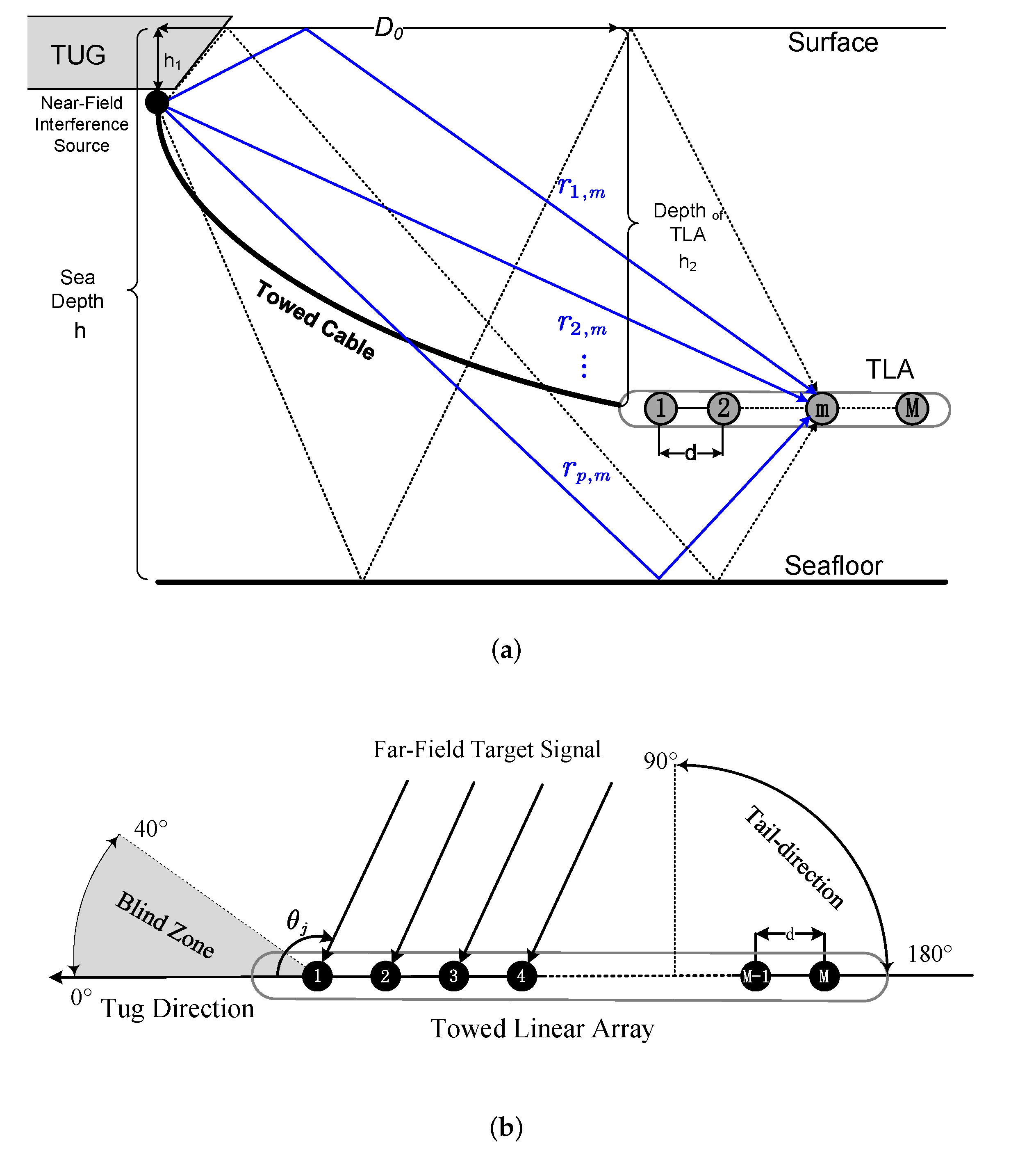
In this paper, a towed linear array, as shown in Figure 1, is considered. It consists of M elements with inter-element spacing d. The aperture of the array is $D=\left(M-1\right)d$. The interference generated by the tug platforms is considered as a single near-field source that emits the interference signal from the end-fire direction of the array. Due to the multi-path propagation from direct transmission and the reflections on the sea surface and floor, the interference signal manifests a certain angle expansion when arriving on the TLA, forming a detection blind zone as shown in Figure 1b. There are J far-field signal sources (targets), with the arrival angle of the j-th target denoted by ${\theta }_j$.

The signal received at the m-th TLA element is given by:

$$x_m\left(t\right)=\sum _{j=1}^J{s}_j\left(t-{\tau }_{j,m}\right)+\sum _{p=1}^P\frac{r_{p,1}}{r_{p,m}}i\left(t-{\tau }_{p,m}\right)+n_m\left(t\right)$$

(1)

where $s_j\left(t\right)$ denotes the j-th far-field target pulse, $i\left(t\right)$ denotes the near-field interfering signal, $n_m\left(t\right)$ denotes the ambient sea noise, and P is the number of propagation paths for the near-field interference source. The ${\tau }_{j,m}$ denotes the relative time delay between the m-th sensor and the first sensor (reference point) for the j-th far-field target source, while ${\tau }_{p,m}$ is the relative time delay between the m-th sensor and the first sensor (reference point) for the p-th path of the interference. The $r_{p,m}$ denotes the length of the p-th path corresponding to the m-th element.

The received signals, $x_m\left(t\right)$, are sampled at a frequency $f_s$ and collected into snapshots each of size L. Applying a L-point fast Fourier transform (FFT) operation on the k-th snapshot leads to:

$$X_m\left({\omega }_l,k\right)=\sum _{j=1}^J{S}_j\left({\omega }_l,k\right)e^{-j{\omega }_l{\tau }_{j,m}}+\sum _{p=1}^P\frac{r_{p,1}}{r_{p,m}}I\left({\omega }_l,k\right)e^{-j{\omega }_l{\tau }_{p,m}}+N_m\left({\omega }_l,k\right)$$

(2)

where ${\omega }_l=2\pi f_l=2\pi \left(l-1\right)f_s/L$. We are interested in the working frequency band $\left[f_{\min },f_{\max }\right]$, corresponding to the index range $l\in [L_1,L_2]$ with $L_1=\lfloor f_{\min }/f_s\rfloor ·L+1$ and $L_2=\lfloor f_{\max }/f_s\rfloor ·L+1$. Collecting the values at ${\omega }_l$ from all M elements leads to $\mathit{X}\left({\omega }_l,k\right)={\left[X_1\left({\omega }_l,k\right),X_2\left({\omega }_l,k\right),\cdots ,X_M\left({\omega }_l,k\right)\right]}^T\in {\mathcal{C}}^{M\times 1}$, which can be expressed as:

$$\begin{array}{c}\hfill \mathit{X}\left({\omega }_l,k\right)=\left[\begin{array}{c}{\mathit{A}}_F\left({\omega }_l,{\mathit{\Theta }}_F\right){\mathit{A}}_N\left({\omega }_l,\mathit{r},{\mathit{\Theta }}_N\right)\end{array}\right]\left[\begin{array}{c}\mathit{S}\left({\omega }_l,k\right)\\ \mathit{I}\left({\omega }_l,k\right)\end{array}\right]+\mathit{N}\left({\omega }_l,k\right)\end{array}$$

(3)

where $\mathit{S}\left({\omega }_l,k\right)={\left[S_1\left({\omega }_l,k\right),\cdots ,S_J\left({\omega }_l,k\right)\right]}^T\in {\mathcal{C}}^{J\times 1}$ and $\mathit{I}\left({\omega }_l,k\right)={\left[I\left({\omega }_l,k\right),\cdots ,I\left({\omega }_l,k\right)\right]}^T$$\in {\mathcal{C}}^{P\times 1}$. The ${\mathit{A}}_F\left({\omega }_l,{\mathit{\Theta }}_F\right)=\left[{\mathit{a}}_F\left({\omega }_l,{\theta }_1\right),{\mathit{a}}_F\left({\omega }_l,{\theta }_2\right),\cdots ,{\mathit{a}}_F\left({\omega }_l,{\theta }_J\right)\right]\in {\mathcal{C}}^{M\times J}$ is called the far-field array manifold, which consists of steering vectors corresponding to the J far-field sources. The j-th steering vector is given as:

$${\mathit{a}}_F\left({\omega }_l,{\theta }_j\right)={\left[1,e^{-j{\omega }_{l}dcos{\theta }_j/c},\cdots ,e^{-j{\omega }_l\left(M-1\right)dcos{\theta }_j/c}\right]}^T$$

(4)

and the near-field array manifold is denoted as ${\mathit{A}}_N\left({\omega }_l,\mathit{r}\right)=\left[{\mathit{a}}_N\left({\omega }_l,r_{p,1}\right),\cdots ,{\mathit{a}}_N\left({\omega }_l,r_{p,M}\right)\right]$$\in {\mathcal{C}}^{M\times P}$, for which the steering vector of the p-th path is:

$${\mathit{a}}_N\left({\omega }_l,r_{p,m}\right)={\left[1,\frac{r_{p,1}}{r_{p,2}}{e}^{-j\frac{{\omega }_l\left(r_{p,2}-r_{p,1}\right)}{c}},\cdots ,\frac{r_{p,1}}{r_{p,M}}{e}^{-j\frac{{\omega }_l\left(r_{p,M}-r_{p,1}\right)}{c}}\right]}^T$$

(5)

This is noted when the near-field interference source is located in the Fresnel region, such that $r\in \left[0.62{\left(D^3/\lambda \right)}^{1/2},2D^2/\lambda \right]$ [15], $r_{p,1}/r_{p,m}\approx 1$.

3. The Proposed Near-Field Interference Suppression Algorithm

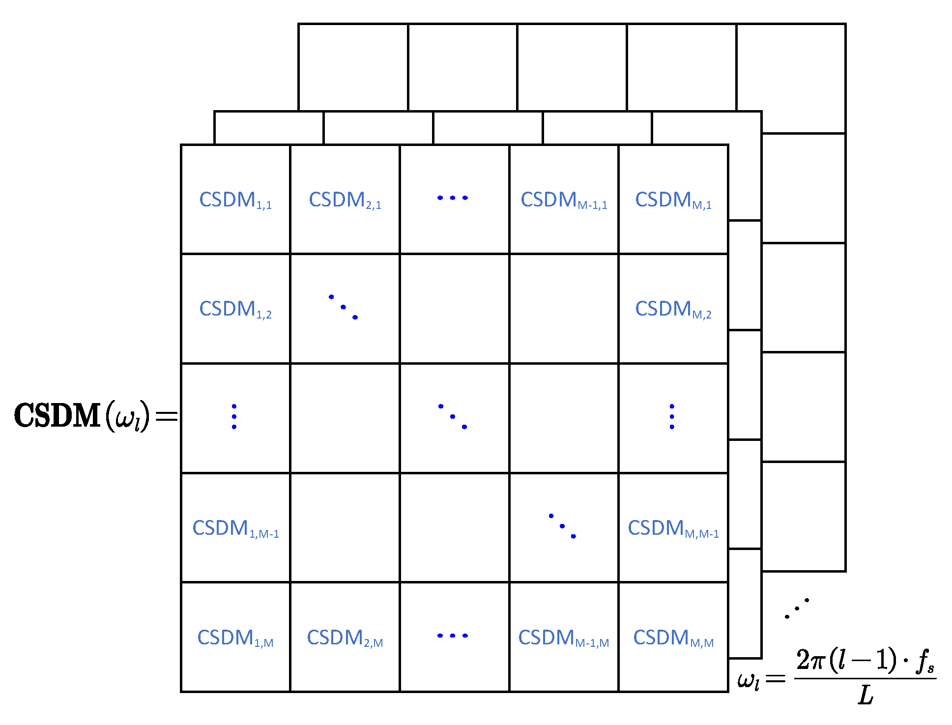
Post-processing beamforming algorithms depend on the cross-spectral density matrix (CSDM), where CSDM is similar to the time-domain cross-correlation, which is used to estimate the correlation between two signals. In addition, CSDM is usually used in signal processing procedures, such as sound source detection, location, and classification [3,4,5,6,7]. The CSDM is constructed by storing the cross-spectral density of each sensor (array element) at all frequencies in the spectrum of interest (together with their complex conjugation and including the self-power spectral density of each sensor on the diagonal). The schematic diagram of CSDM is shown in Figure 2 below.

The key idea of a subspace method such as ECA is to use the covariance matrix of the data received by the array or CSDM to obtain eigenvalues and eigenvectors through eigendecomposition. Then, the subspaces are divided according to certain criteria, including the value size of the eigenvalues and the direction information of the eigenvectors. Subspaces mainly include signal subspace, interference subspace, and noise subspace. The critical step is to eliminate the characteristic components of interference and noise information in the received array data based on the above feature analysis to achieve suppression and improve the signal-to-noise ratio (SNR) and signal-to-interference ratio (SIR). As in the ECA method proposed in [3], the CSDM based on (3) is formed with K snapshots as:

$$\begin{array}{cc}\hfill {\mathit{R}}_x\left({\omega }_l\right)& =\frac{1}{K}\sum _{k=1}^K\mathit{X}\left({\omega }_l,k\right){\mathit{X}}^H\left({\omega }_l,k\right)\hfill \\ \hfill & =\mathit{V}\left({\omega }_l\right)\Lambda \left({\omega }_l\right){\mathit{V}}^H\left({\omega }_l\right)\hfill \\ \hfill & =\sum _{m=1}^M{\lambda }_m\left({\omega }_l\right){\mathit{v}}_m\left({\omega }_l\right){\mathit{v}}_m^H\left({\omega }_l\right)\hfill \end{array}$$

(6)

where the second and third equality are the eigendecomposition of ${\mathit{R}}_x\left({\omega }_l\right)$ in different formats. The $\Lambda \left({\omega }_l\right)$ is a diagonal matrix with eigenvalues $\left\{{\lambda }_m\right\}$ in descending order on its diagonal, $\mathit{V}\left({\omega }_l\right)$ consists of corresponding eigenvectors $\left\{{\mathit{v}}_m\right\}$, and H denotes the conjugate transpose. With the CSDM given in the first equality of (6), the conventional beamforming (CBF) can performed using eigenvector beamforming (EBF), $B_{{\mathit{v}}_m}\left({\omega }_l,\varphi \right)$, as follows:

$$\begin{array}{cc}\hfill & B\left(\varphi \right)=\frac{1}{\Delta L}\sum _{l=L_1}^{L_2}{\mathit{w}}^H\left({\omega }_l,\varphi \right){\mathit{R}}_x\left({\omega }_l\right)\mathit{w}\left({\omega }_l,\varphi \right)\hfill \\ \hfill & =\frac{1}{\Delta L}\sum _{l=L_1}^{L_2}\left(\sum _{m=1}^M{\lambda }_m\left({\omega }_l\right)\left[{\mathit{w}}^H\left({\omega }_l,\varphi \right){\mathit{v}}_m\left({\omega }_l\right){\mathit{v}}_m^H\left({\omega }_l\right)\mathit{w}\left({\omega }_l,\varphi \right)\right]\right)\hfill \\ \hfill & =\frac{1}{\Delta L}\sum _{l=L_1}^{L_2}\left(\sum _{m=1}^M{\lambda }_m\left({\omega }_l\right)B_{{\mathit{v}}_m}\left({\omega }_l,\varphi \right)\right)\hfill \end{array}$$

(7)

where $\Delta L=L_2-L_1$. The weight vector is $\mathit{w}\left({\omega }_l,\varphi \right)={\mathit{a}}_F\left({\omega }_l,\varphi \right)$ with ${\mathit{a}}_F\left({\omega }_l,\varphi \right)$ given by (4) according to [4], such that:

$$B_{{\mathit{v}}_m}\left({\omega }_l,\varphi \right)={\mathit{a}}_F^H\left({\omega }_l,\varphi \right){\mathit{v}}_m\left({\omega }_l\right){\mathit{v}}_m^H\left({\omega }_l\right){\mathit{a}}_F\left({\omega }_l,\varphi \right).$$

(8)

The ECA aims to suppress interferences by subtracting the non-target eigenvectors. To achieve this, it defines the contribution ratio (CR) [3] corresponding to the m-th eigenvector ${\mathit{v}}_m$ as follows:

$$C{R}_{l,m}=\frac{B_{{\mathit{v}}_m}\left({\omega }_l,{\varphi }_0\right)}{\underset{\varphi \in {\mathit{\Phi }}_T}{max}{B}_{{\mathit{v}}_m}\left({\omega }_l,\varphi \right)}$$

(9)

where the bearing of the target of interest (TOI), ${\varphi }_0$, is assumed to be known. The ${\mathit{\Phi }}_T=\left[{\varphi }_{-t}\cdots {\varphi }_{-1}{\varphi }_1\cdots {\varphi }_t\right]$ is the range of suppression, and it consists of t bearings on either side of ${\varphi }_0$. If $C{R}_{l,m}$ is below some threshold, the m-th eigenvector ${\mathit{v}}_m$ is treated as a non-target component. Collecting all non-target eigenvectors, one obtains ${\mathit{V}}_I\left({\omega }_l\right)$, with which a projection matrix is obtained as ${\mathit{P}}_{\perp }\left({\omega }_l\right)=\mathit{I}-{\mathit{V}}_I\left({\omega }_l\right){\mathit{V}}_I^{\mathrm{H}}\left({\omega }_l\right)$. Define:

$${\overline{\mathit{R}}}_x\left({\omega }_l\right)={\mathit{P}}_{\perp }\left({\omega }_l\right){\mathit{R}}_x\left({\omega }_l\right){\mathit{P}}_{\perp }^H\left({\omega }_l\right)$$

(10)

Then, the CBF with interference suppression based on the ECA is obtained as $\overline{B}\left(\varphi \right)=\frac{1}{\Delta L}{\sum }_{l=L_1}^{L_2}{\mathit{a}}_F^{\mathrm{H}}\left({\omega }_l,\varphi \right){\overline{\mathit{R}}}_x\left({\omega }_l\right){\mathit{a}}_F\left({\omega }_l,\varphi \right)$.

The ECA method requires the target bearings to be known in advance, which limits its applications. To address this issue, we propose an enhanced ECA (EECA) method. The basic idea is to divide the eigenvectors at each frequency point into two groups: one denotes non-target eigenvectors and the other includes non-target-only eigenvectors. A non-target eigenvector derives its main contribution from partial noise and partial interference components. A non-target-only eigenvector derives its main contribution from the target subspace, partial noise, and partial interference components. After that, the non-target-only eigenvectors are subtracted from the original CSDM to obtain a new CSDM. Finally, the CBF is performed with a set of new CSDMs to obtain a beam power spectrum, for which we expect the distinct null troughs to appear at the targets’ bearing. Note that the energy of the near-field interference presents a certain space broadening from the far-field perspective. As a result, the distinct null trough does not appear when the partial interference components of the non-target-only eigenvectors are removed.

The key aspect of the EECA scheme is the grouping of eigenvectors. As mentioned, the near-field interference comes from the end-fire direction (bow) of the array. Therefore, it is more feasible to perform a grouping from outside of the blind zone. Without a loss of generality, we rely on the tail-direction zone with a bearing range $\left[90°,180°\right]$, as shown in Figure 1b. The tail-direction zone is divided into Q sectors, denoted as $Q=\lfloor 91/\Delta \varphi \rfloor$. That is, for $q=1,2,\cdots ,Q$, the bearing sector ${\mathit{\Phi }}_q=\left[\Delta \varphi ·\left(q-1\right)+90,\Delta \varphi ·q+90+\lfloor \frac{q}{Q}\rfloor ·\left(91-\Delta \varphi ·q\right)-1\right]$. For the q-th sector, a new CR is defined as:

$$C{R}_{q,l,m}=\frac{\underset{\varphi \in {\mathit{\Phi }}_q}{max}{B}_{v_m}\left({\omega }_l,\varphi \right)}{\underset{\varphi \in \left[0°,180°\right]}{max}{B}_{v_m}\left({\omega }_l,\varphi \right)}$$

(11)

Supposing that ${\mathit{\Phi }}_q$ is the non-target sector, we have the following classification:

• If $C{R}_{q,l,m}=1$, then ${\mathit{v}}_m\left({\omega }_l,q\right)\in {\mathit{V}}_N\left({\omega }_l,q\right)$;
• If $C{R}_{q,l,m}<1$, then ${\mathit{v}}_m\left({\omega }_l,q\right)\in {\mathit{V}}_T\left({\omega }_l,q\right)$.

The ${\mathit{V}}_N\left({\omega }_l,q\right)$ denotes the non-target subspace already defined, and the ${\mathit{V}}_T\left({\omega }_l,q\right)$ is the non-target-only subspace. Similar to (10), we define:

$${\tilde{\mathit{R}}}_x\left({\omega }_l,q\right)={\tilde{\mathit{P}}}_{\perp }\left({\omega }_l,q\right){\mathit{R}}_x\left({\omega }_l,q\right){\tilde{\mathit{P}}}_{\perp }^H\left({\omega }_l,q\right)$$

(12)

where ${\tilde{\mathit{P}}}_{\perp }\left({\omega }_l,q\right)=\mathit{I}-{\mathit{V}}_T\left({\omega }_l,q\right){\mathit{V}}_T^H\left({\omega }_l,q\right)$. Based on (12), a beam power spectrum is obtained as follows:

$${\tilde{B}}_{\mathrm{EECA}}\left(\varphi ,q\right)=\frac{1}{\Delta L}\sum _{l=L_1}^{L_2}{\mathit{a}}_F^H\left({\omega }_l,\varphi \right){\tilde{\mathit{R}}}_x\left({\omega }_l,q\right){\mathit{a}}_F\left({\omega }_l,\varphi \right)$$

(13)

Based on (13), one obtains: For the current q-th sector, we obtain:

$$\begin{array}{cc}\hfill {\widehat{\varphi }}_{\max }\left(q\right)& =\underset{\varphi \in \left[0°,180°\right]}{\arg \max }{\tilde{B}}_{\mathrm{EECA}}\left(\varphi ,q\right)\hfill \\ \hfill {\widehat{\varphi }}_{\min }\left(q\right)& =\underset{\varphi \in \left[0°,180°\right]}{\arg \min }{\tilde{B}}_{\mathrm{EECA}}\left(\varphi ,q\right)\hfill \end{array}$$

(14)

If the following two conditions are met:

• C1: The –3 dB beamwidth of the lobe centered at ${\widehat{\varphi }}_{\max }\left(q\right)$, ${\beta }_q^{-3dB}$, is larger than a predefined threshold—that is, ${\beta }_q^{-3dB}>{\gamma }_{\beta }$—which indicates that the current beam directivity is weak;
• C2: The ${\widehat{\varphi }}_{\min }\left(q\right)\notin {\mathit{\Phi }}_q$ and the depth of the null trough at ${\widehat{\varphi }}_{\min }\left(q\right)$, $D_q$, is larger than a predefined threshold—that is, $D_q>{\gamma }_D$.

Then, we decide the current sector ${\mathit{\Phi }}_q$ is a non-target sector we need, and there is a target at the bearing ${\widehat{\varphi }}_{\min }\left(q\right)$. Furthermore, we scan the entire power spectrum for other null troughs as potential targets. The proposed EECA scheme is finally summarized in Algorithm 1.

Algorithm 1: The proposed EECA scheme.

Initialization:

Set the number of sectors Q;

for (l from $L_1$ to $L_2$) do

Calculate the CSDM ${\mathit{R}}_x\left({\omega }_l\right)$ and perform eigendecomposition to obtain the eigenvector matrix $\mathit{V}\left({\omega }_l\right)$;

end for

Loop:

for (q from 1 to Q) do

for (l from $L_1$ to $L_2$) do

for (m from 1 to M) do

Calculate the $C{R}_{q,l,m}$ according to (11);

If $C{R}_{q,l,m}<1$ then ${\mathit{v}}_m\left({\omega }_l,q\right)\in {\mathit{V}}_T\left({\omega }_l,q\right)$.

end for

Obtain the ${\tilde{\mathit{R}}}_x\left({\omega }_l,q\right)$ as (12)

end for

Obtain the ${\tilde{B}}_{\mathrm{EECA}}\left(\varphi ,q\right)$ as (13), base on which ${\widehat{\varphi }}_{\max }\left(q\right)$, ${\widehat{\varphi }}_{\min }\left(q\right)$, ${\beta }_q^{-3dB}$ and $D_q$ are determined.

if ${\beta }_q^{-3dB}>{\gamma }_{\beta }$ and $D_q>{\gamma }_D$ then

Found the targets at ${\widehat{\varphi }}_{\min }\left(q\right)$ and other bearings with other null troughs in ${\tilde{B}}_{\mathrm{EECA}}\left(\varphi ,q\right)$;

Break out of the loop of q.

else

Continue with the loop of q.

end if

end for

4. Simulations

In this section, it is assumed that the far-field targets and the near-field interference exist simultaneously in the space and no other far-field interference, where the noise is additive random noise. Furthermore, the TOI’s bearing in ECA and MUSIC-IS is assumed to be known in advance. The simulations are presented to show the performance of the proposed EECA method, with the relevant parameters listed in

Table 1. Parameter setting table.

Basic Parameters
Number of Elements (M)	48	Element Spacing (d)	0.75 m
Sound Speed (c)	1500 m/s	Sampling Frequency ($F_s$)	10 KHz
Sampling Duration ($t_s$)	0.1536 s	FFT bins	256
Frequency of Interest	[100 Hz, 1000 Hz]
Sea Depth (h)	150 m	Interference Source Depth ($h_1$)	5 m
Horizontal Distance ($D_0$)	400 m	TLA Deployed Depth ($h_2$)	25 m
Scenario I—Signal/Interference Parameter Setting
	Bearing (${\theta }_1$)	Frequency ($f_1$)	SNR
Target Signal 1	25${}^{\circ }$	750 Hz	−20 dB
	Bearing (${\theta }_2$)	Frequency ($f_2$)	SNR
Target Signal 2	124${}^{\circ }$	500 Hz	−20 dB
	Frequency (f)	SIR
Interfering Signal	120 Hz	−25 dB
Scenario II—Signal/Interference Parameter Setting
	Bearing (${\theta }_1$)	Frequency ($f_1$)	SNR
Target Signal 1	15${}^{\circ }$	300 Hz	−20 dB
	Bearing (${\theta }_2$)	Frequency ($f_2$)	SNR
Target Signal 2	24${}^{\circ }$	750 Hz	−20 dB
	Frequency (f)	SIR
Interfering Signal	150 Hz	−25 dB

.

A 48-element TLA with a spacing of $d=0.75$ m was considered. The speed of sound was $c=1500$ m/s. The frequency of interest was $[100,1000]$ Hz, over which the number of investigated frequency bins was $L=256$. The sampling frequency was $f_s=10$ kHz, and the sampling data had a time duration of $t_s=0.1536$ s. For the tail-direction scanning, the sector size of ${\mathit{\Phi }}_q$ was set as $\Delta \phi =3°$, and the scanning resolution was 1°, leading to $Q=30$.

The sea depth was $h=150$ m. In Scenario I, two far-field targets at bearings 25 and 124, respectively, were considered. The continuous wave (CW) signal from the two targets had frequencies of 750 and 500 Hz, respectively, at a signal-to-noise ratio (SNR) of −20 dB. The near-field interfering source had a depth of $h_1=5$ m, radiating interference signal at a frequency of 120 Hz. The signal-to-interference ratio (SIR) was −25 dB. The deployed depth of the TLA was $h_2=25$ m, and the horizontal distance between the near-field interference source and the first array element was $D_0=400$ m.

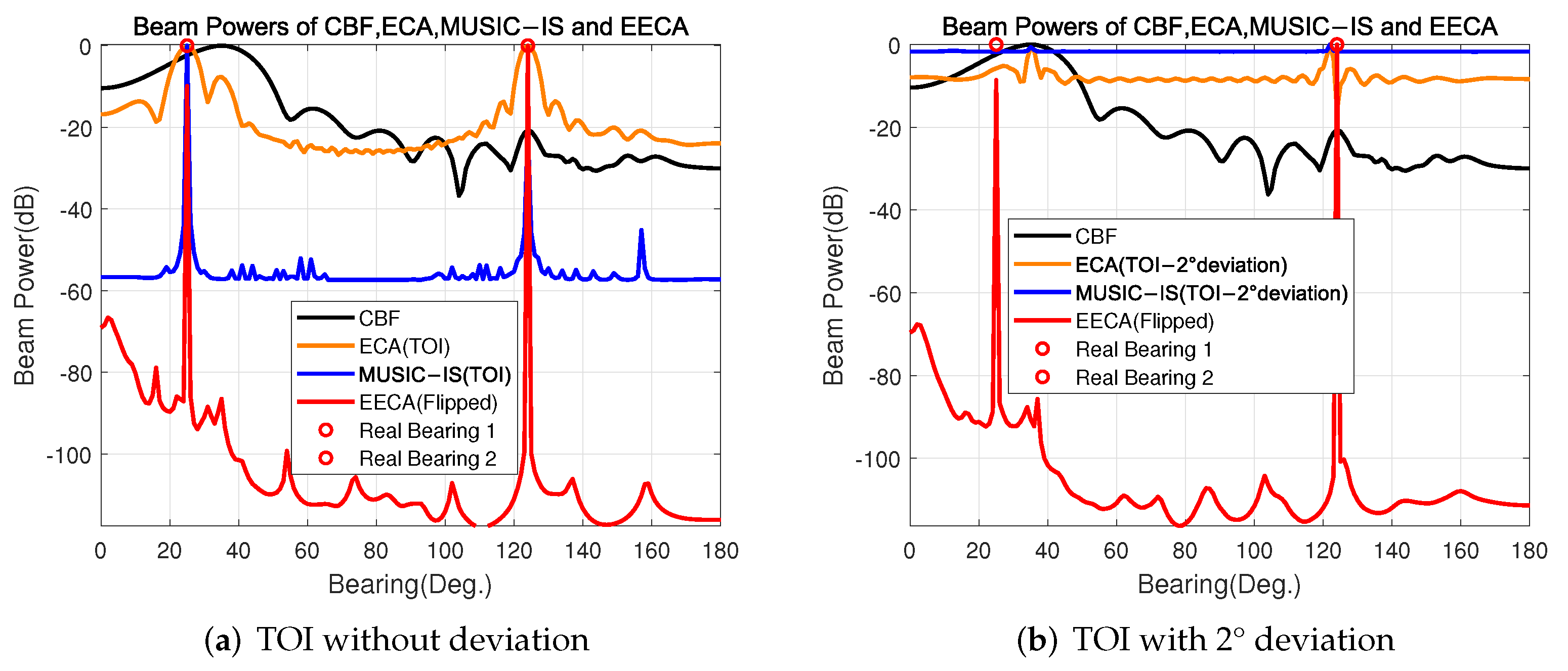
The beam power spectra of the CBF, ECA, MUSIC-IS, and proposed EECA in Scenario I are shown in Figure 3, where the EECA curve is the flipped version of that given by (13).

The bearing range of suppression for the ECA, ${\mathit{\Phi }}_T$, is extended to the entire region for a fair comparison. From the figure, the CBF fails to obtain the DOA estimation of far-field sources due to the influence of strong near-field interferences. Specifically, the target from the 25° that falls into the blind zone is thus completely masked. For the target from the 124°, there is a peak at a very low level that is difficult to identify. The ECA method, assuming the target bearings are known, achieves a decent spatial spectrum, as expected. Because of the better angle resolution and estimation accuracy of the MUSIC-based method, when the bearings of TOI are known, the result in Figure 3a indicates that MUSIC-IS can obtain a better interference suppression effect and a higher output SNR. However, as shown in Figure 3b, when the bearings of TOI have a certain deviation, the ECA and the MUSIC-IS cannot accurately obtain the non-target subspace, resulting in the failure of the DOA estimation. Regarding the EECA, there are two sharp spikes located at the target bearings, indicating its excellent suppression of the near-field interference, even for the target in the detection blind zone. Compared with the ECA and MUSIC-IS, the output SNR is dramatically improved. The EECA method is based on ECA, making it easy to implement and inheriting its advantages. Although the tail-scanning procedure increases the computational load to a certain extent, for ECA and MUSIC-IS the performance of EECA is far superior in the absence of prior information.

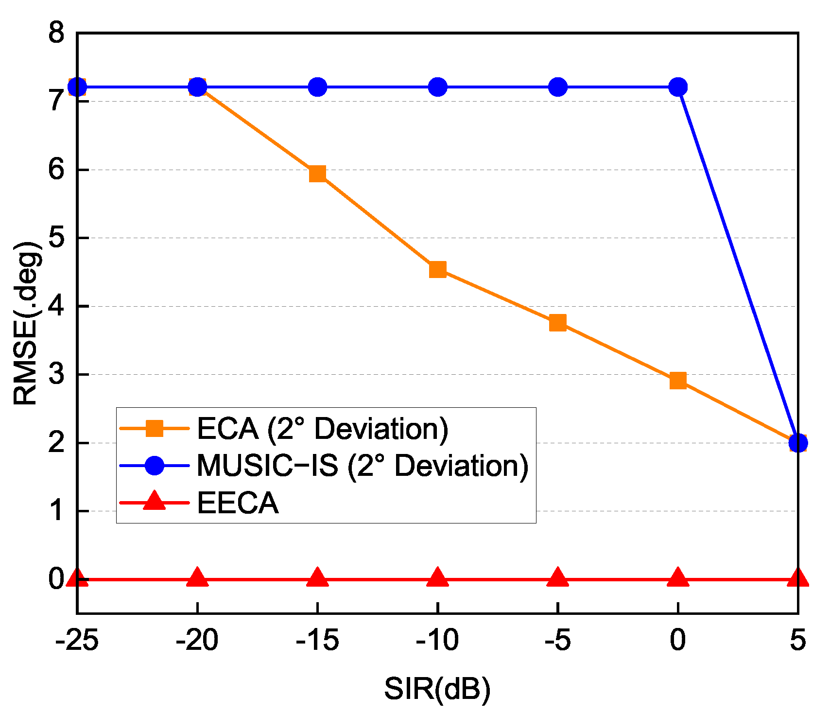
Then, we study the root mean square error (RMSE) versus SIR in Scenario I, for which the calculation of RMSE is based on the following equation [15]:

$${\mathrm{RMSE}}_{\theta }=\sqrt{\frac{{\sum }_{n=1}^{N_{mc}}{\sum }_{j=1}^J{\left({\widehat{\theta }}_{ji}-{\theta }_j\right)}^2}{N_{mc}·J}}$$

(15)

where $N_{mc}$ denotes the number of Monte Carlo trials and ${\widehat{\theta }}_{ji}$ denotes the DOA estimation of the j-th target in the i-th trial. The results are shown in Figure 4, where for each SIR point, 200 Monte Carlo trials were performed. As shown, the EECA provides an accurate estimate of the TOI’s bearing even at a low SIR level. The ECA and the MUSIC-IS suffer significant performance loss even for a small deviation in the TOI’s bearing. Furthermore, when the bearing of TOI is without deviation, the DOA estimates the performances of ECA and MUSIC-IS to be equal to the EECA; thus, they are not plotted repeatedly.

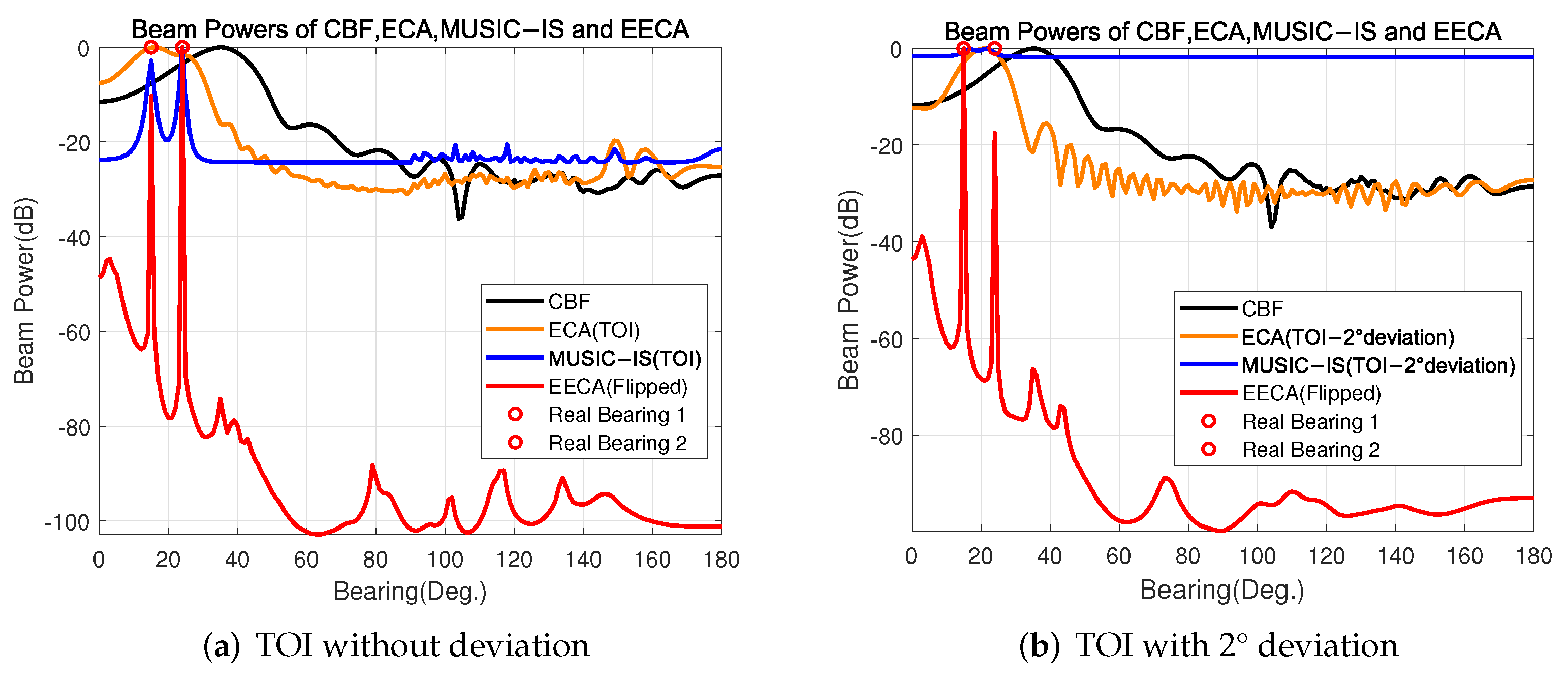
In Scenario II, the two far-field targets at bearings 15° and 24°, respectively, were both considered in the detection blind zone. The continuous wave (CW) signal from the two targets had frequencies of 300 and 750 Hz, respectively, at an SNR of −20 dB. The radiating interference signal had a frequency 150 Hz. The SIR was −25 dB. The beam power spectra of the CBF, ECA, MUSIC-IS, and proposed EECA in Scenario II are shown in Figure 5.

From the figure, it can be seen that the CBF fails to obtain DOA estimation of far-field sources due to the influence of strong near-field interferences. Specifically, the ECA method also fails on the premise that TOI is with or without bearing deviation. The situation is different for the MUSIC-IS. When the TOI’s bearing is accurately known, the interference suppression performance of MUSIC-IS is better than that of ECA. However, when the bearing deviation of TOI exists, the MUSIC-IS fails to realize the DOA estimation. As for the EECA, the two sharp spikes indicate its excellent interference suppression performance in the non-cooperative scenario.

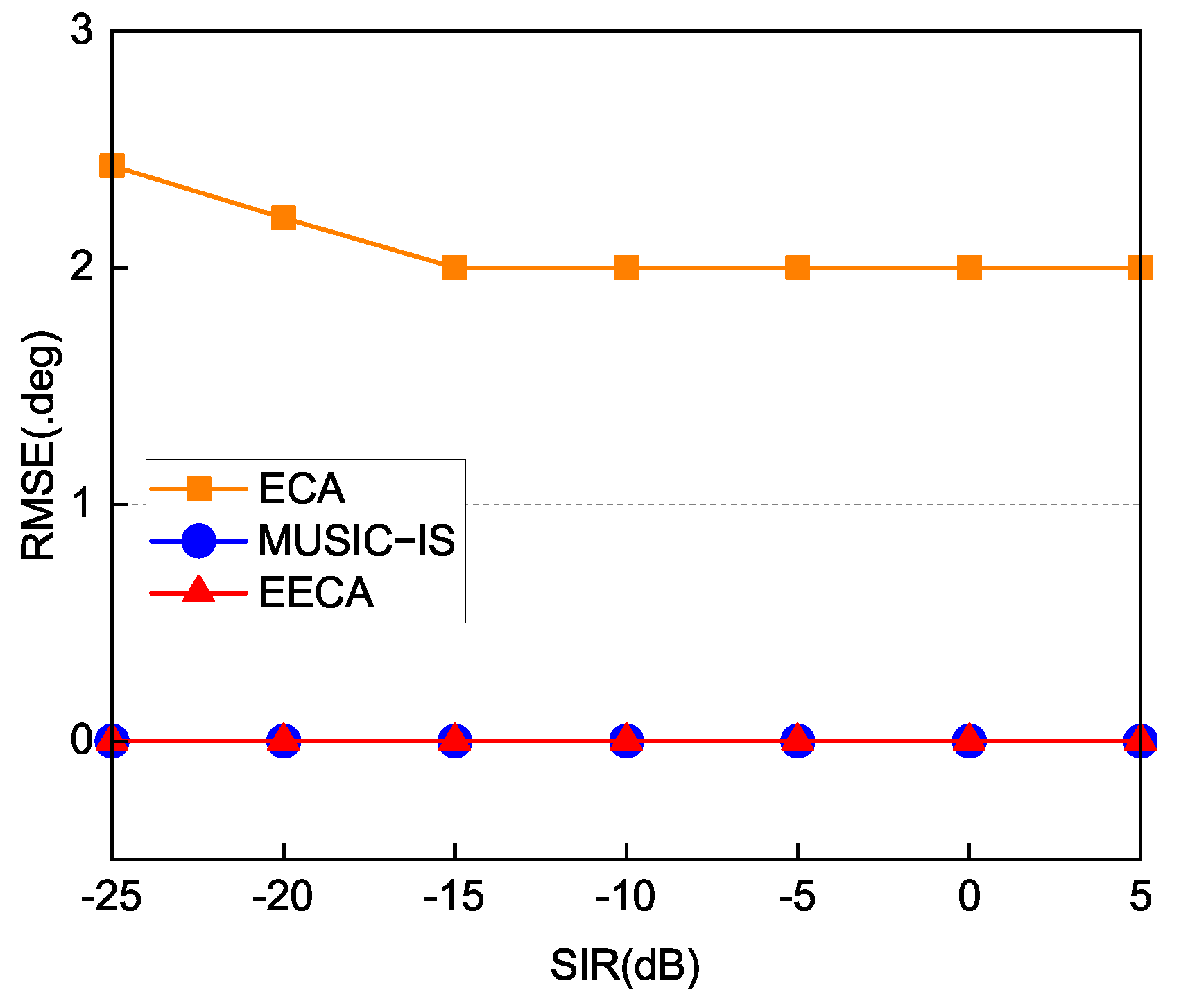
Similarly, we also studied the RMSE versus SIR in Scenario II. The results are shown in Figure 6, where, for each SIR point, 200 Monte Carlo trials were performed. Unlike the results in scenario I, where the ECA method suffered a dramatic performance decline under extreme conditions, the performance of MUSIC-IS was acceptable when the TOI’s bearing was known without deviation, and the EECA method remained robust. Note that when the bearing of TOI deviates, the ECA and MUSIC-IS cannot distinguish the target; therefore, they are not shown in the figure.

5. Conclusions

In this paper, an enhanced near-field interference suppression scheme based on an existing eigencomponent association (ECA) method for a towed linear array (TLA) was proposed. By seeking a non-target sector in the tail-direction zone of the TLA, interference suppression was achieved without requiring any prior knowledge. The issue of target recognition in the detection blind zone of the TLA was also solved. Although EECA increases the computational load to a certain extent, the method is easy to implement and has excellent performance in non-cooperative scenarios. The numerical results show that the proposed EECA significantly outperforms the ECA and the MUSIC-IS by dozens of dB processing gains and can achieve target interception even when the SIR is −25 dB.