Understanding the Settling Processes of Dredged Sediment Disposed in Open Waters through Experimental Tests and Numerical Simulations

Abstract

During dredging for subsea tunnels and pipelines, the dredged soil is typically dumped in a designated area. Understanding the settling behaviors of the dumped particles is essential for an accurate prediction of the resulting morphology. This study dealt with the settling processes in the open-water column by means of experimental tests and numerical simulations. Both quiescent and ambient current conditions were taken into account. Particular attention was paid to the induced flow patterns, descent sediment movement features and the resulting topography. Regarding the diffusion width and settling velocity, three key effect factors, i.e., dumped volume, particle size and ambient flow strength, were considered. The results show that the dumped sediment in the water forms a particle cloud, and two vortices with opposite rotations occur on both sides of the cloud. During settlement, three stages corresponding to convective descent, dynamic collapse and passive diffusion are observed. Most of the descending sediment is incorporated in a spherical vortex, resembling an upside-down mushroom cloud, and some sediment is also contained in an irregular trailing stem. The dumped particles exhibit initial acceleration, and then they slow down to converge to a fixed value. Subjected to the ambient currents, the initial acceleration phase is prolonged, and the vortex is somewhat distorted; the particle cloud is also advected downstream with a velocity roughly equal to the ambient current.

1. Introduction

Open-water sediment disposal is common in many applications associated with both coastal and offshore areas around the world, including land reclamation, coastline extension and contaminated sediment isolation. Large quantities of dredged soils are often produced in the construction of harbors, subsea tunnels and pipelines, etc. Usually, the dredged material is dumped directly by a suction dredger in a designated area [1,2]. The dumping process is accompanied by sediment diffusion, which may bring about some environmental issues. As required by environmental protection and design optimization, higher dumping standards, in terms of the smoothness or gradient of underwater sediment mounds, have been put forward [3,4,5,6]. To achieve an ideal morphology and meet the standards after dumping, the traditional method is to measure the generated topography with multi-beam technics, and then to shape the topography by excavation-filling construction [7]. Understanding the sediment settling patterns is helpful for the prediction of the resulting morphology, so that the expected topography is achieved with a minimal workload.

During the dumping, a large amount of sediment enters the water in a relatively short time, and hyper-concentrated flow is thereby generated. Compared with single-particle movement, a large cluster of particles stirs the flow, which causes the flow and sediment transport patterns to be significantly different from the behaviors in the natural water column [8]. Distinct from one-phase flow (Bingham fluid) and high-viscous debris, the hyper-concentrated flow with non-viscous particles belongs to a turbulent two-phase flow, in which the density gradient, lift effect and particle collision all exhibit some certain particularities.

By means of field observations, many researchers have carried out a significant amount of work on sediment dumping, of which the focus was the settling processes and the accumulation mechanism of particles [7]. In 1973, the U.S. Army Corps, as the pioneer, conducted a long-term tracer test of a dredging project in Sonoma Bay, San Francisco, and systematically provided the transportation, diffusion and deposition laws of dredged sediment [9]. Later, some scholars from the United States, Japan and Europe also performed a series of prototype observations on the movement of dredged materials after being dumped in open waters [10,11,12,13,14,15]. These observations provided some insight into the special phenomenon with respect to the dumped sediment diffusion and settlement in the water. However, limited by the measuring instruments and test conditions, the observed phenomenon was not profound, and the recorded data were not well documented. The dumping process is a relatively short-term activity, which is not easy to be captured regarding the instantaneous shape changes at each moment. Therefore, laboratory experiments and numerical simulations, as alternatives, could complement each other and provide insights into the processes.

Through laboratory experiments, Rahimipour and Wilkinson [16] analyzed particle clouds using sheet illumination to expose the internal structure of particle clouds composed of graded sand and initial volumes. They captured the descent velocity of particle clouds and found that these velocities were comparable with those found for a miscible thermal of the same radius and buoyancy. Ruggaber [17] analyzed the physical mechanisms for sediment losses on the basis of the characteristic cloud behavior as it descended in the water column. In his experiments, the focus was on how realistic modes and variables of sediment disposal operations (e.g., particle size, water content and initial momentum) affected cloud behavior. Gu et al. [18] performed an experimental study on unsorted particle clouds discharged into a cross-flow, and they found that clouds exhibited significant differences compared with the stagnant ambient case. To observe the fate of sediments released instantaneously in a current, Genscheimer et al. [19] performed flow visualization experiments in a glass-walled recirculating flume. Most available experiments have been performed in quiescent conditions. However, water bodies in nature are not quiescent; instead, they are continually under the influence of surface waves and time-varying (e.g., tidal) currents. Documenting particle settling behavior in ambient currents is thus desirable.

In a simulation of the dumping process, Koh and Chang first developed a short-term mathematical model for the prediction of the dispersion and settlement of waste material discharged into the ocean [20]. Based on the short-term model, Brandsma and Divkoy developed two short-term models to explore the instantaneous and continuous dumping process [21]. With the assistance of the model established by Koh and Chang, Han et al. speculated the covering range of the settled particles and calculated the deviation distance of the resulting topography [22]. During the settlement process, they found that an internal vortex played a certain role in the decrease in particle concentration. The horizontal transport effect of advection was appreciable, which was consistent with the results of Huang et al. [23]. There were some shortages in these models, which assumed that the particles touched the bottom and formed a semi-ellipsoid pattern. However, this assumption differs from the reality that the particles should move radially outward as a density-driven surge.

When simulating the dumping process, it is normally regarded as point source diffusion in the convection–diffusion equation [24,25,26,27,28]. The total particles are weighted and distributed to each calculation cell at one time, which is reasonable for the diffusion of fine sediment. However, the movement of water and coarse particles belongs to a solid–liquid two-phase flow [29,30]. During the settlement, the diffusion model does not fully solve the movement of the two-phase flow. Moreover, in a fluctuated water column, the settlement is significantly affected by the interaction of the particles and the turbulence, which is a complex nonlinear process [31]. The movement of particles enhances or weakens the flow turbulence somehow; the varied turbulence, in turn, affects the settlement [32,33,34,35].

This study deals with the settling process of dredged particles through experimental tests and numerical modeling, paying attention to the flow patterns, the settlement and diffusion of particles and the formation process of sediment accumulation. The experiments were carried out under both stationary water and moving flow conditions. Considering the interaction of water and sediment, a coupling of the two-phase flow model was developed and validated based on the measured data. This research provides some preliminary results in terms of the diffusion width, settling velocity and resulting topography. The complement of both methods helps to understand the settling behaviors of sediment clouds, providing a reference for dredging sediment disposal in similar situations.

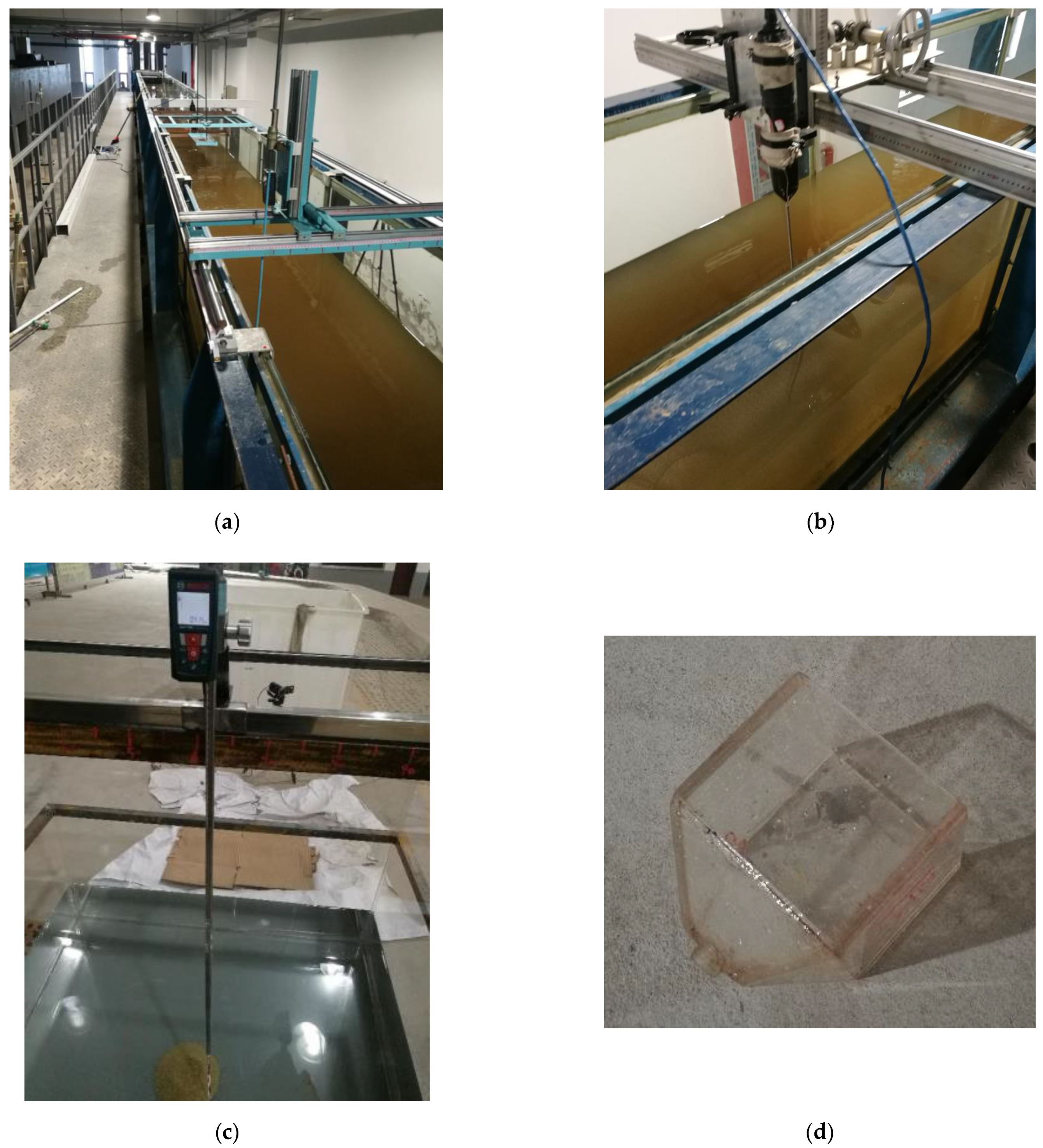
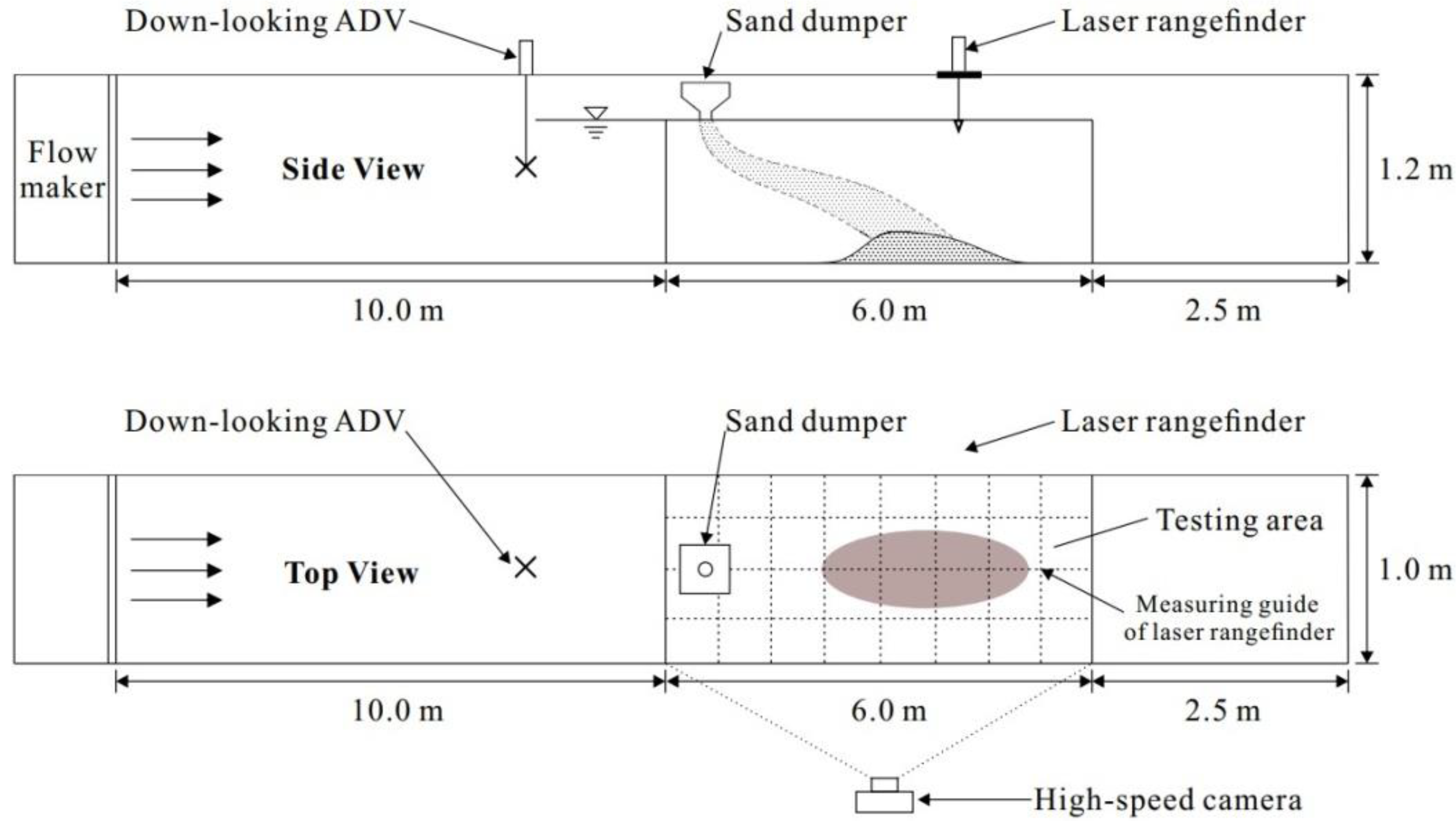
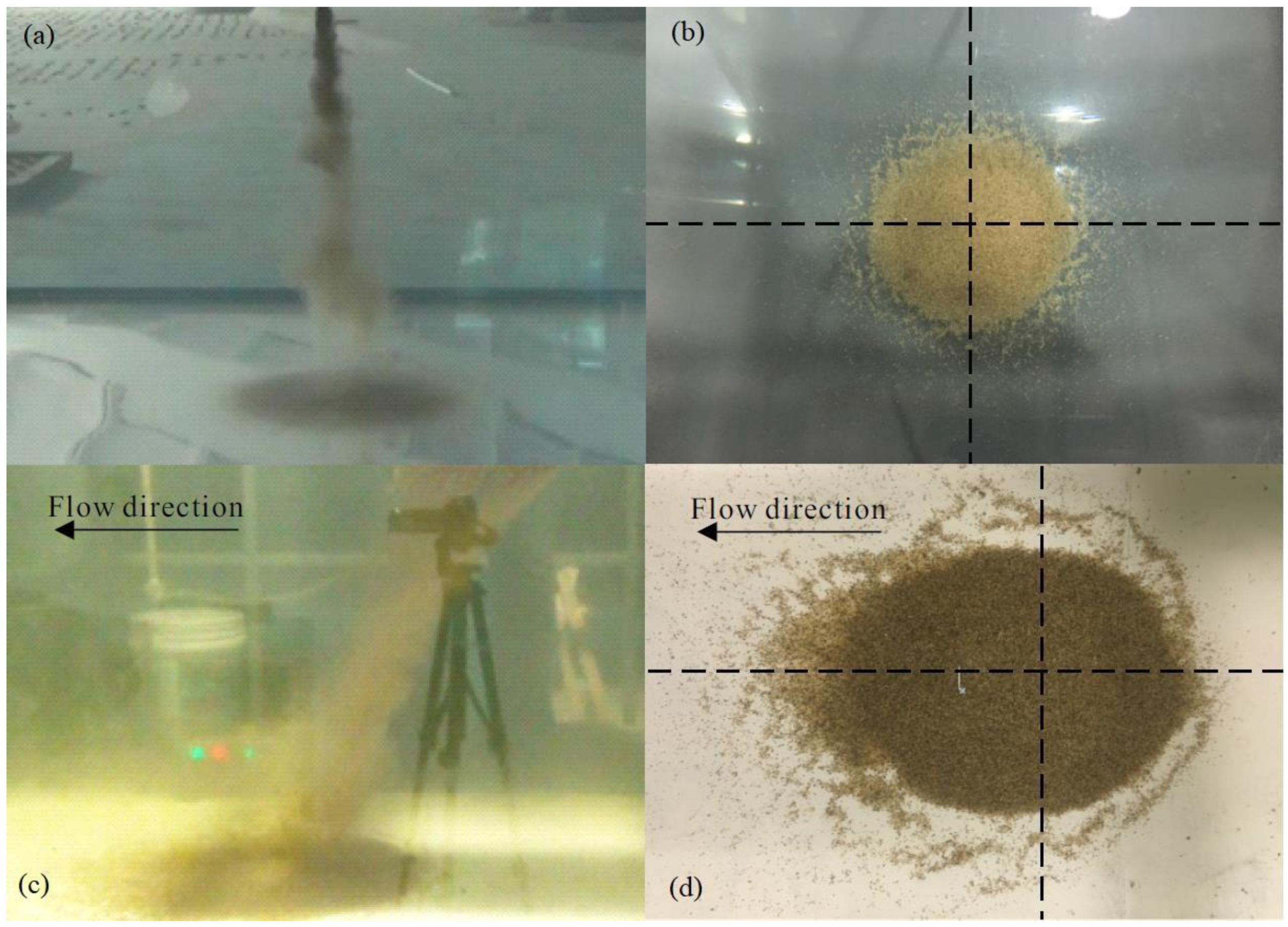
2. Experimental Tests

The experimental tests were conducted in a flume at the Nanjing Hydraulic Research Institute (NHRI). Figure 1 shows some photos of the experiment, and a schematic layout of the experimental setup is shown in Figure 2. The flume was 18.5 m long, 1.0 m wide and 1.2 m high. Its sidewalls and bottom plates were made of plexiglass, allowing visualization. The test area was situated some 10.0 m downstream of the inlet. The sand dumper was attached at the upper part of the area and fixed immediately over the flume, allowing for all of the release conditions to be performed in a ‘point’-style release. Its nozzle diameter was 0.8 cm. The bottom edge of the nozzle was set at the same level as the water surface, and the particles fell freely from the dumper and entered the water column. The release mechanism was successfully used for releases of sediment with different particle sizes, released at different elevations. At the flume inlet, a pump with an electromagnetic flowmeter was equipped to supply a regular or random flow. To measure the flow velocities, an acoustic Doppler velocimeter (ADV) was installed 3.0 m upstream of the sand dumper, and the measurement error was 0.10 cm/s. A laser rangefinder was adopted to measure the micro-topography with an accuracy of ±0.5 cm. At the outlet, a tailgate regulated the water stage. On the right side of the flume, a high-speed camera was installed at a 2.0 m distance from the test area; instantaneous flow images were captured at a 10 Hz frequency; and the duration for data collection was 10 s. To ensure that the height/width ratio had a negligible effect on the settling processes and the formation of underwater mounds, pre-experimental tests were carried out in the available flume to determine the choice of test particles, dumped volume and flow velocity.

In the process of the dumping experiments, two water conditions were considered, i.e., stationary state and moving flow. The former refers to the dumped particles’ movement being driven only by gravity and buoyancy in the vertical direction; the latter means that the movement is also affected by the horizontal flow motion [36]. To relate the research in the laboratory to open-water sediment disposal in the field as much as possible, realistic sediment particles from field collections were used. Three types of natural sand were selected for the experimental tests, in which the medium grain size D₅₀ = 0.40, 0.70 and 1.0 mm. Figure 3 shows the grain size distribution. Moreover, the uniformity coefficient C_u and the curvature coefficient C_c are also essential factors. According to the laboratory analysis, the C_c values were ~1.0, while the C_u values were >1.0. However, before the tests, to improve their uniformity, we also used a sand vibrating screen to further screen the sediment particles. Therefore, in the present experiments, the effects of C_u and C_c on the settling processes were not taken into account, while the focus lay on the grain size, i.e., D₅₀.

There were 74 cases in total, in terms of varied water depth H, D₅₀, sediment volume V, sediment density ρ_s and flow velocity U, performed for tests under the two flow conditions. U is the horizontal velocity measured by the ADV at 0.6H. More details are available in Luo et al. [37]. In this paper, 9 cases were chosen for illustration, as shown in

Table 1. Experimental flow and sediment conditions.

Case	D50 (mm)	H (cm)	V (cm3)	ρs (kg/m3)	U (m/s)
1	0.40	50	1000	1430	0
2	0.40	70	1000	1430	0
3	0.40	90	1000	1430	0
4	0.70	90	1000	1720	0
5	1.00	90	1000	1928	0
6	0.40	90	1000	1430	0.05
7	0.40	90	1000	1430	0.08
8	0.40	90	1000	1430	0.10
9	1.00	90	1000	1928	0.05

. Zero velocity means the flow is regarded as still/quiescent. In some practical engineering conditions, e.g., in the presence of a cofferdam, the water column during the dumping processes is almost static. In this regard, the cases where the flow velocity is approximately zero (Cases 1−5) were also considered for analysis. The amount of dumped sand was determined using a preparatory test to ensure that the sidewall effect on the particle settlement was minimized. The sediment was dumped into the water column at a steady rate, i.e., in a given period, t_p, the total dumped volume was V. The rate of dumping remained the same in all the experimental tests, ~16.7 cm³/s. It would take ~60 s for the material to be completely dumped. The sediment dumping was at a roughly constant rate irrespective of the ambient currents. Considering that, during practical engineering, the dumping activity is supposed to be carried out at relatively weak ambient current conditions, the maximum flow velocity usually does not exceed 0.10 m/s [7].

To measure the flow and sediment movement in the flume, challenges do exist, especially during the initial stage of sand dumping, which is mainly ascribed to the turbulence enhancement in a short time and sediment diffusion in a dramatic manner. Despite this, measurements were repeated 2−3 times to guarantee the accuracy.

3. Numerical Simulations

The movement of water and sediment belongs to a solid–liquid two-phase flow. To simulate the settling processes, a mathematical model of two-phase flow was first established, which is composed of several differential equations describing the momentum and continuity. On the basis of the flow model, particle movement was added for the coupling solution. In given boundary and initial conditions, the model is solved with the finite difference method.

3.1. Mathematical Formulation

Based on the Navier–Stokes equations of the fractional/area volume (FAVOR) grid method, the flow continuity and momentum equations were established. The volume fraction was introduced into the continuity equation to track the interface between the particles and the water:

$$V_F\frac{\partial \rho }{\partial t}+\frac{\partial }{\partial x}(\rho u{A}_x)+\frac{\partial }{\partial y}(\rho v{A}_y)+\frac{\partial }{\partial z}(\rho w{A}_y)=R_D+R_S$$

(1)

where V_F is the fractional volume open to flow; u, v and w are the velocity components in the x, y and z coordinates, respectively; A_x, A_y and A_z are the corresponding fractional areas in the x, y and z directions; R_D and R_s are the turbulent diffusion term and mass source, respectively; ρ is the water density; and t is time.

The derived 3D momentum equations with some additional terms are

$$\frac{\partial u}{\partial t}+\frac{1}{V_F}\left\{u{A}_x\frac{\partial u}{\partial x}+v{A}_y\frac{\partial u}{\partial y}+w{A}_z\frac{\partial u}{\partial z}\right\}=-\frac{1}{\rho }\frac{\partial p}{\partial x}+G_x+f_x-b_x-\frac{R_S}{\rho V_F}(u-u_w-u_s)$$

(2)

$$\frac{\partial v}{\partial t}+\frac{1}{V_F}\left\{u{A}_x\frac{\partial v}{\partial x}+v{A}_y\frac{\partial v}{\partial y}+w{A}_z\frac{\partial v}{\partial z}\right\}=-\frac{1}{\rho }(\frac{\partial p}{\partial y})+G_y+f_y-b_y-\frac{R_S}{\rho V_F}(v-v_w-v_s)$$

(3)

$$\frac{\partial w}{\partial t}+\frac{1}{V_F}\left\{u{A}_x\frac{\partial w}{\partial x}+v{A}_y\frac{\partial w}{\partial y}+w{A}_z\frac{\partial w}{\partial z}\right\}=-\frac{1}{\rho }\frac{\partial p}{\partial z}+G_z+f_z-b_z-\frac{R_S}{\rho V_F}(w-w_w-w_s)$$

(4)

where G_x, G_y and G_z are body accelerations; f_x, f_y and f_z are viscous accelerations; b_x, b_y and b_z are flow losses, and the final terms account for the injection of mass at a source represented by a geometry component; u_w, v_w and w_w are the velocity components of the source; u_s, v_s and w_s are the fluid velocities at the source surface relative to the source itself; and p is the pressure.

For compressible flow, the internal energy equation is

$$V_F\frac{\partial }{\partial t}(\rho I)+\frac{\partial }{\partial x}(\rho Iu{A}_x)+\frac{\partial }{\partial y}(\rho Iv{A}_y)+\frac{\partial }{\partial z}(\rho Iw{A}_z)=R_D+R_S-p\left\{\frac{\partial u{A}_x}{\partial x}+\frac{\partial v{A}_y}{\partial y}+\frac{\partial w{A}_z}{\partial z}\right\}$$

(5)

where I is the internal energy of the macroscopic mixture. For two-fluid flow,

$$\rho I=F{\rho }_w{I}_w+(1-F){\rho }_s{I}_s$$

(6)

where F is the volume fraction of the fluid, and the indices indicate quantities related to the fluid or solid.

To solve the derived momentum equations, the turbulence model is used for closure. Commonly used turbulence models include the k-ε model, k-ɷ model, Plante mixing length model and renormalization group model (RNG). By comparison, the RNG model has wider applicability for the calculation of low-intensity turbulent flows [38,39]. Therefore, it was adopted:

$$\frac{\partial {\epsilon }_T}{\partial t}+\frac{1}{V_F}\{u{A}_x\frac{\partial {\epsilon }_T}{\partial x}+v{A}_y\frac{\partial {\epsilon }_T}{\partial x}+v{A}_z\frac{\partial {\epsilon }_T}{\partial z}\}={\kappa }_1\frac{{\epsilon }_T}{k_T}(P_T+{\kappa }_3{G}_T)+Dif{f}_{\epsilon }-{\kappa }_2\frac{{\epsilon }_T^2}{k_T}$$

(7)

where $P_T$ is the turbulent kinetic energy production term; $G_T$ is the buoyancy production term; $Dif{f}_{\epsilon }$ is the diffusion term; ${\kappa }_1$, ${\kappa }_2$ and ${\kappa }_3$ are dimensionless parameters, where the values are 1.44, 1.92 and 0.2, respectively; ${\epsilon }_T$ is the rate of turbulent energy dissipation; and $k_T$ is the turbulent kinetic energy, expressed as

$${\epsilon }_T=\frac{u_{*}^3}{K_a}$$

(8)

$$k_T=\frac{u_{*}^2}{0.3}$$

(9)

where $u_{*}$ is the local shear velocity, which is determined as

$$u_0=u_{*}\left[\frac{1}{K_a}\ln (\frac{\rho }{\mu }{u}_{*}d)+5.0\right]$$

(10)

where u₀ is the parallel component of the velocity adjacent to the wall at a distance d, and K_a = 0.4 is the von Karman constant.

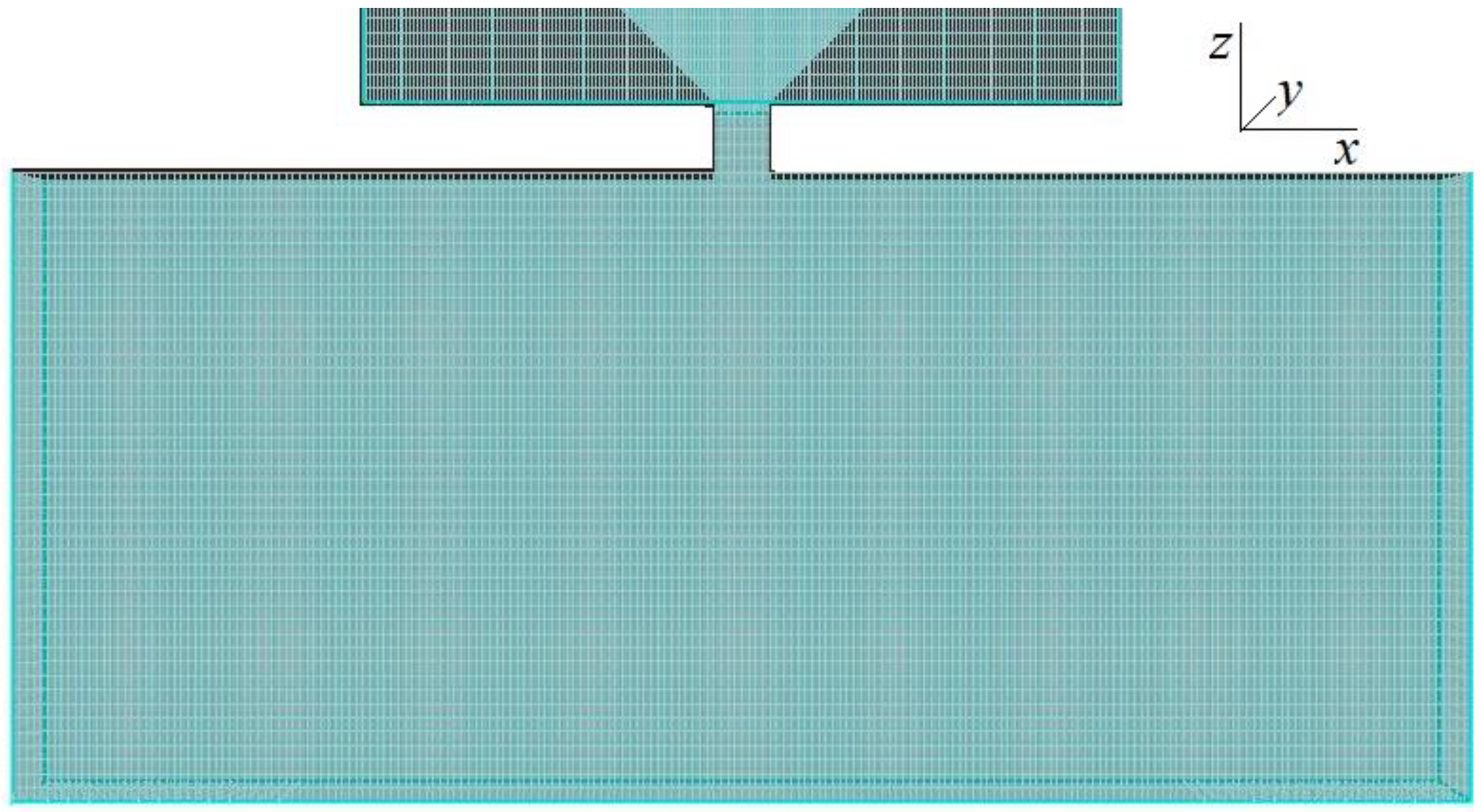
3.2. Mesh and Boundary Conditions

The computations were performed in the same size as in the experimental studies. Starting with a coarse mesh, global and local refinements were carried out to achieve a fine mesh. Figure 4 shows the computational grid. Several meshes of varied cell sizes were evaluated to ensure grid independence, which was checked through steady-state calculations. The domain was finally covered by 800,000 hexahedron cells. Smaller cells, with a 0.01 m size, were used in the test area to account for large velocity gradients.

The numerical simulations were also performed at the two water conditions, i.e., static water and moving flow. During the settling processes, to simulate the changes in the cloud width and the settling velocity, the initial dumped volume is specified in the numerical model for illustration. The simulated flow and sediment conditions are listed in

Table 2. Simulated flow and sediment conditions.

Case	D50 (mm)	V0 (cm3)	ρs (kg/m3)	U (m/s)
1	0.40	4.0	1430	0
2	0.40	6.0	1430	0
3	0.40	8.0	1430	0
4	0.70	6.0	1720	0
5	1.00	6.0	1928	0
6	0.40	6.0	1430	0.05
7	0.40	6.0	1430	0.08
8	0.40	6.0	1430	0.10
9	1.00	6.0	1928	0.05

, in which V₀ is the initial dumped volume.

Regarding the boundary conditions, at the inlet, the lateral constant inflow was specified, i.e., a uniform velocity is maintained. With respect to the boundary value, it is typically assumed that there is a local equilibrium between the turbulent shear generation term and the dissipation term, that is, ${\epsilon }_T=k_T$. At the outlet, a fully developed turbulent flow was defined, i.e., the vertical velocity is zero. On the water surface, the free surface was selected using the rigid cover assumption, and the normal gradient of each quantity was zero. On the bottom, the non-slip boundary condition was adopted implying that there is no bed sediment exchange.

3.3. Numerical Parameters

The experimental tests show that the accuracy of sand dumping is closely related to the degree of settlement and diffusion of the particles. A schematic diagram and photo of sediment settlement are shown in Figure 5. The figure illustrates that, before touching the bottom, the descent of the leading edge of the sediment cloud determines the covering range of the underwater particles to a certain extent.

The particle clouds in moving flows can exhibit significant differences when compared with the stagnant ambient case [18,19]. The difference is quantified by analyzing the longitudinal width of the cloud between the left-most and right-most longitudinal edges, L_d, and the dumping period t_p. The non-dimensional forms of these parameters are

$$L_{md}=L_d/l_s$$

(11)

$$t_d=t_p/t_s$$

(12)

where l_s = V₀^1/3 is a length dimension, and t_s is a time dimension. Considering the influence of gravity, density difference and dumped sediment volume, it is expressed as follows:

$$t_s=t_p{}^{-1/2}\Delta {\rho }^{-1/2}{V}_0^{1/6}$$

(13)

$$\Delta \rho =({\rho }_s-\rho )/\rho$$

(14)

4. Results and Discussion

Under both quiescent and ambient current conditions, the dynamics of the particles in terms of the settling process and the flow patterns were analyzed. Comparisons were made between the measurements and simulations regarding the resulting morphology. With respect to the diffusion width and settling velocity, the key effect factors including the dumped volume, particle grain size and ambient flow velocity were taken into account.

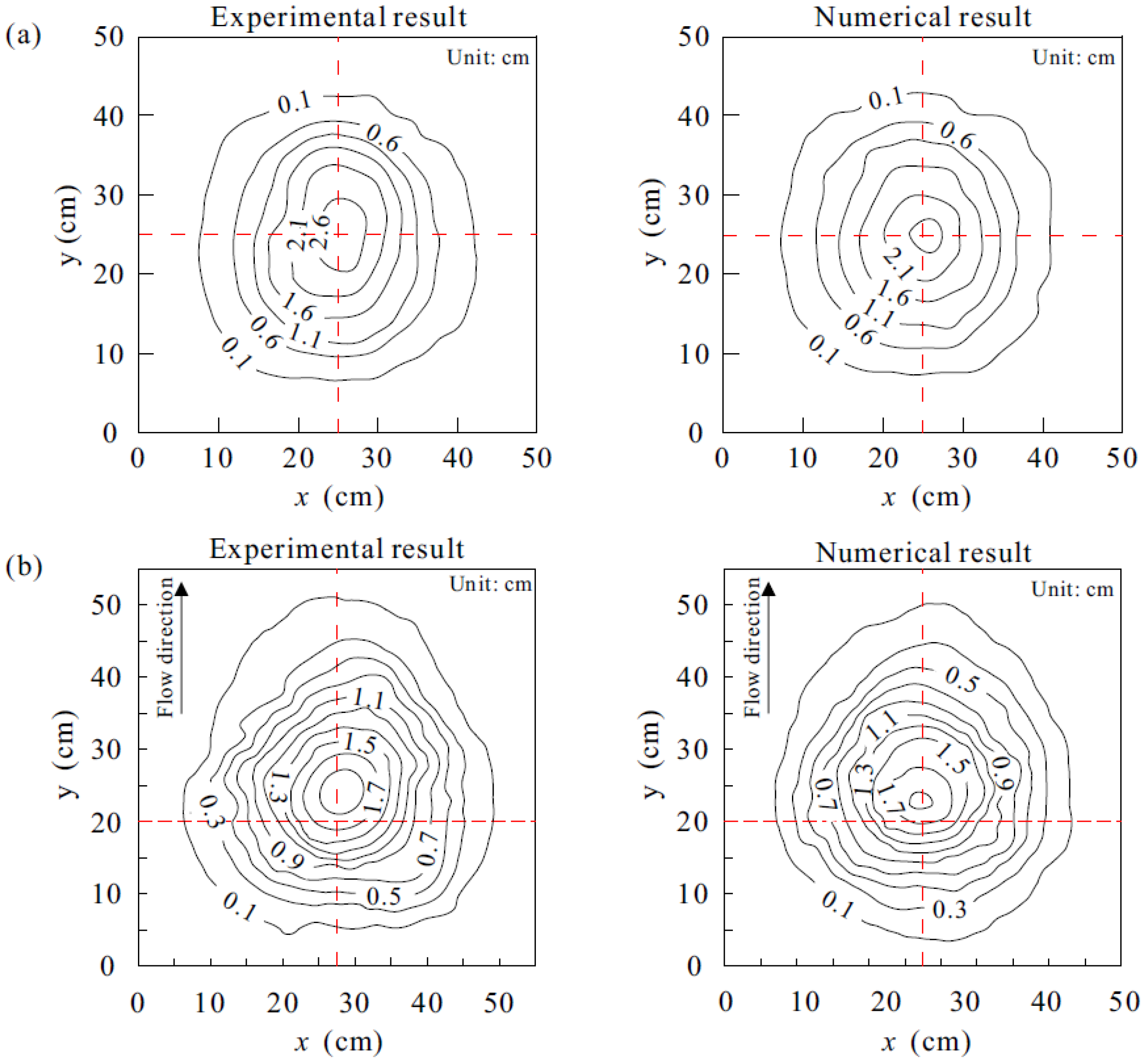
4.1. Comparision between Experimental and Numerical Results

To illustrate the sediment dumping and the resulting morphology in the experimental tests, two cases were chosen corresponding to Case 5 and Case 9. Figure 6a,b present the dumping in the static water column, where D₅₀ = 1.00 mm, H = 90 cm and V = 1000 cm³. It shows that sediment that is dumped in a quasi-instantaneous manner, driven by gravity, forms a particle cloud. In the process of vertical settlement, the sediment exhibits some diffusion in the horizontal direction. The particles touch the bottom and generate a relative cone-shape mound; the formed mound is nearly symmetrical in space. The introduction of the ambient currents (U = 0.05 m/s) makes the process significantly different from the one in the quiescent state, as shown in Figure 6c,d. The particles settle down vertically and, meanwhile, also advect streamwise, which is mainly ascribed to the flow motion. Unidentical to the cone shape, the formed mound has a large length in the flow direction, and it forms a volcanic cone on the top, which is consistent with the field observations [7] and the laboratory measurements [37].

The resulting morphology after dumping, as an essential index, can reflect the sediment cloud movement in the water column. Therefore, for validation of the developed model, the simulated morphology, in the form of contour lines, was compared with the measurements, as shown in Figure 7. The thickness of the sediment accumulation at the outer edge is nearly zero; however, it is not easy to measure the thickness below 0.001 m in the experiments, which is limited by the capability of the laser rangefinder. As a result, the contour lines at 0.1 cm and above were selected for comparison. Figure 7 shows that, in the two water conditions, the simulated profiles are in relatively good agreement with the measured ones, and the overall shapes of the resulting topography are similar. In the stationary state, the particles settle within a radius of 17 cm around the drop site. In the moving flow, the particles are deposited within a radius of 25 cm. Considering that the simulated morphology is roughly consistent with the measurements, it also indicates that the developed model including the adoption of the RNG model is suitable in the simulations of particles moving in a low-intensity turbulent flow.

According to the simulation results, regardless of the existence of ambient currents, the radiation range is slightly reduced, and the peak of the accumulation body is steeper. In addition, under the action of the moving flow, the peak position is further downstream than the actual measured value, and the slope on the backside is also larger. The primary reason is that the size of the sediment particles in the experiments could not be completely consistent. The settling velocity of a particle, w₀, in a liquid can be estimated using Stokes’ law [40], i.e., $w_0=\left({\rho }_s-{\rho }_w\right)g{D}_{50}^2/18\mu$. From the formula, we could find that the coarse-grained sediment with large particle sizes has a larger settling velocity, and as a result, it settles in the upstream more rapidly than the fine-grained sediment. The fine sediment that is smaller than the D₅₀ settles further downstream due to the flow movement, and this phenomenon has a certain randomness. Further, the initial condition of the model is that a certain sediment density is specified at the dumper nozzle, and the upper boundary is assumed to be a steel cover. In the physical experiments, it is difficult to accurately describe the impact of sediment on the water body when it entered the water. In addition, when the boundary conditions are set, a non-slip boundary condition is adopted near the bottom layer, and there is no bed surface sediment exchange. As a result, the sediment would not continue to transport after reaching the bottom. Hence, the center offset distance and accumulation range of the particles would be smaller than the measured data. According to the observations, the avalanche-like process usually occurring in the air does not happen during the continuous dumping on the existing pile of sediments. This is because the flow entrainment effect is more pronounced when the particles settle to the bottom, and in this process, the existing pile does not reach the critical angle of repose.

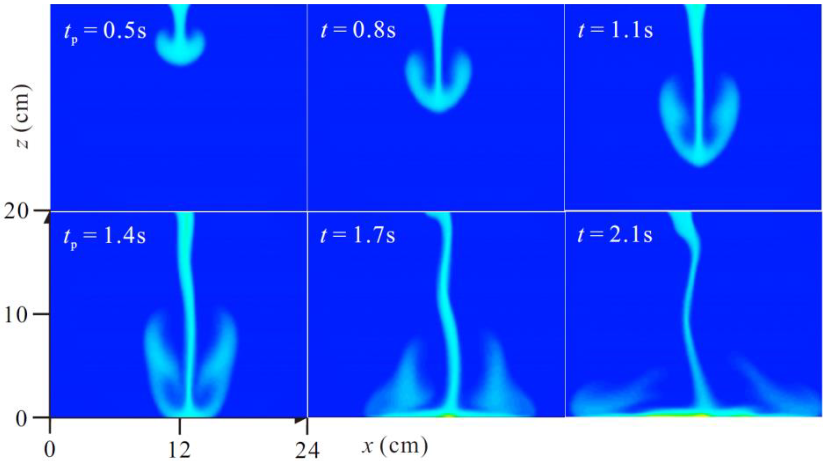
4.2. Settling Process of the Particles

To illustrate the settling process of the particles, the two same cases, i.e., Cases 5 and 9, were selected for analysis, corresponding to the quiescent and ambient current conditions, respectively. In the static water column, Figure 8 shows the simulated settlement process of the particles, in which six moments were selected for illustration. As we can see, at t = 0.5 s, the sediment that is initially released in a quasi-instantaneous manner forms a particle cloud driven by gravity. This is because the motion results from the buoyancy of the particles, and, in some ways, it resembles a thermal produced by the release of a buoyant liquid, where the word ‘thermal’ is used to describe certain aspects of the cloud motion. There are three different stages of a descending particle cloud: (1) convective descent, (2) dynamic collapse and (3) passive diffusion [14,20,21,39]. Each phase contributes to the long-term fate of the released material, but the dynamics of particle clouds and the short-term fate of released material take place in the first phase. In the self-preserving phase at t = 0.9 and 1.3 s, most of the sediment is incorporated in a spherical vortex, resembling an upside-down mushroom cloud, sometimes referred to as a ‘cap,’ or ‘parent cloud.’ However, some sediment is also contained in an irregular ‘trailing stem’. This also shows that, with the elapsed time, driven by gravity, the particle clouds keep settling, and as a result, the stem becomes longer and slimmer. This is mainly caused by the sediment advection–diffusion during the settling process. It is suggested that this observation is not associated with the size of the nozzle. Even if the nozzles are smaller than a particular size, it would not give the stem zero width. It is obvious that during the stage, both settlement and diffusion play a role at the same time; the sediment clouds diffuse with the relative movement of the water column, accompanied by settlement until reaching the bottom. In the dynamic collapse phase, e.g., t = 1.7 s, the particles reach the bottom and collapse; there is a process of quick diffusion and reflection on both sides, that is, the process of ‘dynamic dissipation’. During the process of horizontal expansion, e.g., t = 2.1 and 2.5 s, the average concentration gradually decreases. In the process of settlement, the sediment cloud in the space exhibits certain symmetrical movement features. The process is consistent with the observations of Johanson [14] and Truitt [41].

In the circumstances of ambient currents, it is discovered that the current has a significant influence on the formation of the sediment cloud, which forms when particles are released into the water column, as shown in Figure 9. There are also three different stages of a descending particle cloud, similar to that in a static water column. The currents are characterized by the presence of a spherical vortex that forms at a similar depth and grows to a similar size when compared with particle clouds in quiescent conditions. The introduction of the current appears to prolong the initial acceleration phase and distort the spherical vortex, e.g., from t = 0.5 to 1.1 s. This is because, during the vertical acceleration stage, the particles also move in the horizontal direction driven by the current. As a result, to reach the terminal velocity, the needed acceleration time becomes longer. When the particles touch the bottom and diffuse to the surroundings, e.g., from t = 1.4 to 2.1 s, the ambient currents enhance the mixing of the particles and the current, leading to an increase in the diffusion range. Although the diffusion range at the bottom increases, the relative density between the particles and the current declines; as a result, the diffusion after hitting the bottom becomes relatively weaker compared with that in the static water column. Gensheimer et al. performed flow visualization experiments and observed the fate of sediments released instantaneously in a current; they also found that, in weak ambient currents, particle clouds were advected downstream with a velocity equal to the ambient current, but otherwise, their behavior and structure were similar to those in quiescent conditions [19].

Comparing Figure 8 and Figure 9, the resulting cloud at t = 1.3 s with U = 0 is similar to that at t = 1.1s with U = 0.05 m/s. This is because during the initial settlement stage, the density of particles is high and the impact of ambient currents is comparatively small; as a result, the horizontal movement is not significant but it does occur, while as the settlement progresses further, the particles are diffused by the turbulent action of the flow, and the ambient currents play an essential role, which makes the resulting cloud different from that in the quiescent water column.

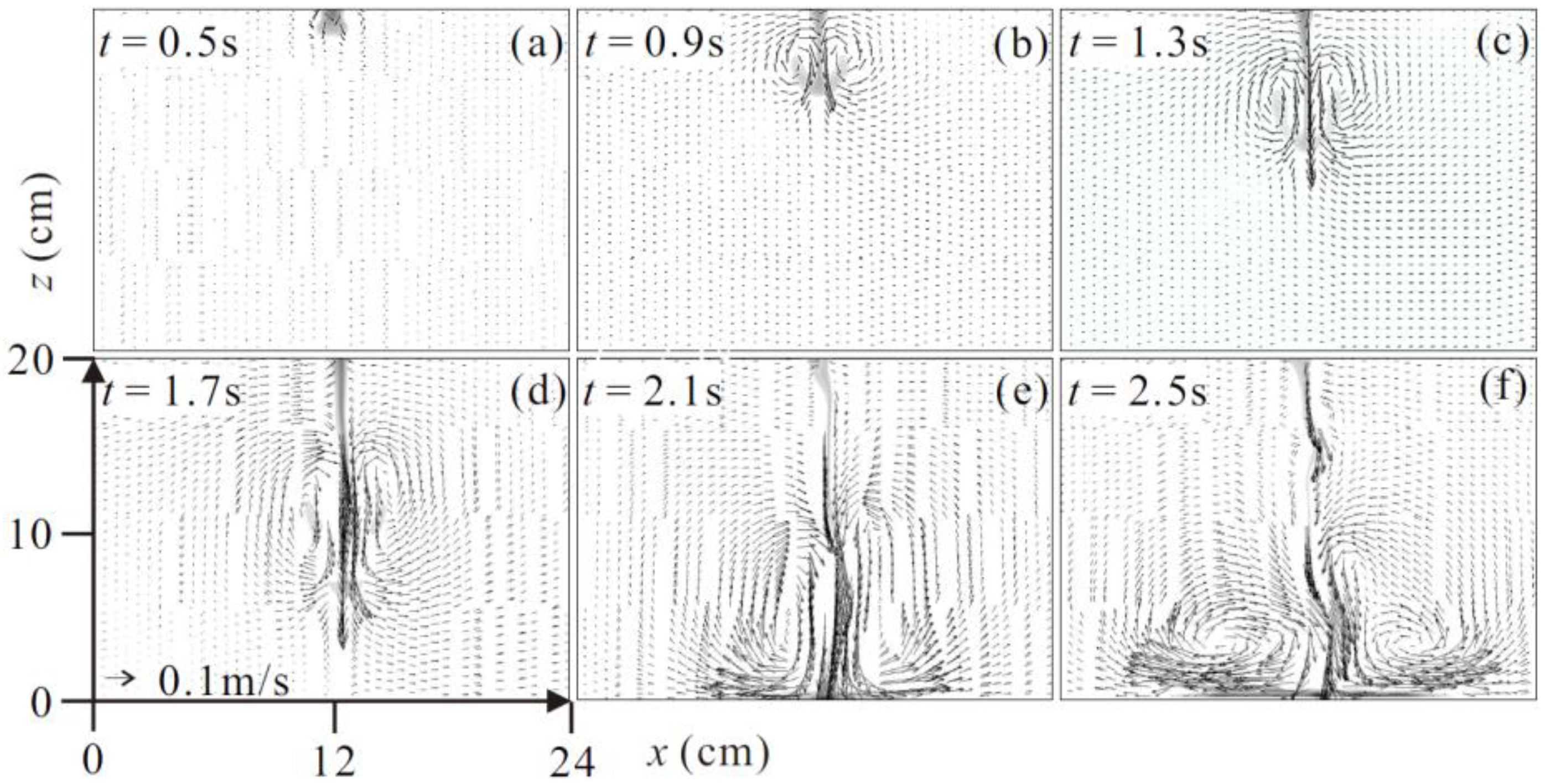
4.3. Flow Pattern Analysis

The sediment is dumped into the water column and significantly stirs the water in both magnitude and direction. During the dumping, a large amount of sediment is released in a short time, leading to strong turbulence in the surrounding water column and therefore generating a vertical flow movement. The flow and sediment mix interplay with each other, presenting irregularly instant patterns [7]. To illustrate the flow patterns during the dumpling, the same two aforementioned cases were chosen for analysis.

Figure 10 displays, in the static water column, the flow fields in the process of particle settlement. In Figure 10a, the sediment is initially released, and in the meantime, vortices on both sides of the particles begin to appear; in the process of settling, e.g., in Figure 10b–d, the two vortices, rotating in the opposite directions, expand gradually. During the processes, most of the particles are incorporated in the spherical vortices; as a result, the upside-down mushroom cloud and the irregular trailing stem are generated. The vortices have a blocking effect on the particle cloud; the symmetrical movement leads to a split in the cloud, and the surface shear force generated by the pressure gradients enhances the horizontal diffusion, as shown in Figure 10d. As the particles reach the bottom, e.g., in Figure 10e,f, the spherical vortices become distorted, and there is an apparent increase in the growth of the cloud length. In the process of vertical settlement, the overall flow velocities in the water column are significantly enhanced, and especially in the surrounding of the particles, the water is significantly stirred.

Figure 11 presents, in the moving flow (U = 0.05 m/s), the flow fields in the process of particle settlement. With the introduction of the ambient currents, the two vortices rotating in the opposite direction also appear after the particles enter the water column, but the vortices are unsymmetrical compared with those in quiescent conditions. Driven by the flow, the upstream vortex moves downward faster than the downstream vortex; during the gradual settlement, the intensity of vortices is continuously enhanced, and their vertical ranges are also expanded at the same time, as shown in Figure 11a–d. The intensity difference of the two vortices leads to the advection of the sediment cloud. As the particles reach the bottom, e.g., in Figure 11e,f, similar to the bottom flow patterns in static water, the spherical vortices in the moving flow also show distortion, and there is a noticeable augmentation in the growth of the cloud length. This phenomenon is mainly qualitative and could only be observed for smaller particle sizes because of limitations on the maximum current speed that should be considered during the experimental setup (preferably < 0.10 m/s) [19].

The particles’ movement is connected to the flow patterns. Compared with the particle clouds in the quiescent environment, the clouds in the ambient currents experience greater growth in longitudinal width and a reduced descent velocity, especially after the initial acceleration stage. Gu et al. [18] attributed the reduced descent velocities to the fact that the spherical vortex is either damaged or destroyed. They also concluded that mixing between the particle cloud and ambient fluid is enhanced. Their observations and measured experimental data are in agreement with the results presented in this paper.

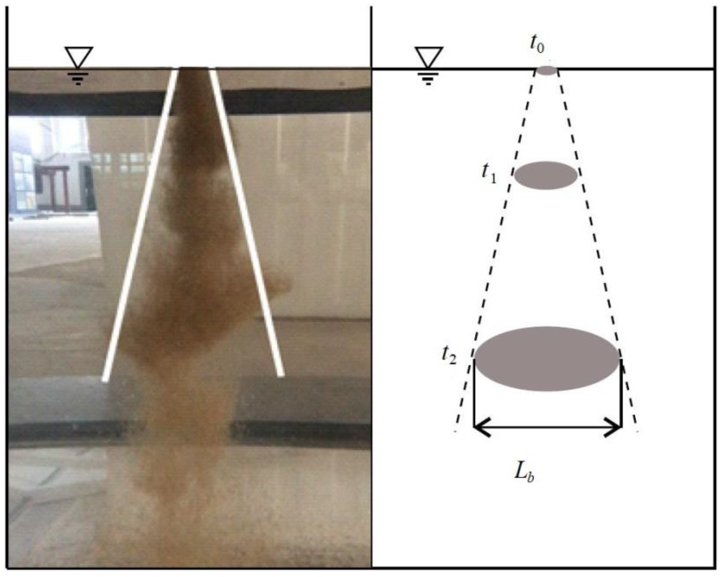
4.4. Diffusion Width

The diffusion width L_md of the sediment clouds is a result of the combined gravity settlement and turbulent diffusion [42]. In flume experiments, it is difficult to determine the L_md, which is limited by the definition of the cloud edge. In this study, with reference to the initial particle concentration, the location with a concentration lower than 5% is defined as the edge of the clouds. The initial particle concentration refers to the pre-dumped sediment density; the particles do not mix with the water, and the density is determined by the particles themselves. The local sediment concentration means the post-dumped density per unit volume; the particles enter the water column and mix with the water, and the concentration is associated with both the water body and the sediment. To illustrate the L_md variations, three parameters in terms of initial dumped volume V₀, D₅₀ and flow velocity U were selected for analysis. The results were compared with the measurements from Scorer [43] and Li [44].

Figure 12a presents the effects of the V₀ on the L_md changes with the elapsed time, in which V₀ = 4, 6 and 8 cm³, corresponding to Cases 1, 2 and 3, respectively, as shown in Table 2. The figure shows that all the calculated L_md values are within the upper and lower limits from Li [44] and also in line with Scorer’s result [43], indicating a relatively good model performance. The L_md shows an increasing trend as the V₀ increases. As expected, a larger group of particles shows quick diffusions. Figure 12b displays the effects of the D₅₀ on the L_md changes, in which D₅₀ = 0.4, 0.7 and 1.0 mm, corresponding to Cases 2, 4 and 5, respectively. The figure shows that the L_md declines with an augmentation of the D₅₀. This is because the bigger particles often have a larger settling velocity, and therefore, in the process of large particles settling, the vertical movement plays the dominant role compared to its horizontal diffusion.

Under the action of ambient currents, it is also discovered that the strength of the current has a significant influence on the L_md variations, as shown in Figure 12c. Increasing the current speeds (U = 0, 0.05, 0.08 and 0.10 m/s) appears to expand the diffusion ranges. This is explained by the fact that the strength of the current affects the formation of the clouds, which form when particles are released into the water. The increase in the current speed prolongs the initial acceleration phase and distorts the spherical vortex, thereby enhancing the turbulence in the surrounding of the particles. As a result, the L_md is amplified when the strength of the ambient current is further increased. Overall, during the initial stage of the settlement, the L_md increases approximately in a linear way, and the growth rate then declines gradually with the elapsed time.

4.5. Settling Velocity

The particle cloud’s settling velocity, w, is defined as the vertical velocity of its leading edge. In the process of settlement, the induced flow patterns in the surrounding of the cloud are complex; limited by the flow measurement technology, there is little research available focusing on w analysis. As mentioned before, two vortices exist on both sides of the particles, which leads to the uneven pressure distributions outside the particle clouds; as a result, some particles could easily escape from the clouds and diffuse into the surrounding flow. This makes it difficult to capture the leading edge and the w as well. Moreover, the settlement takes place in a relatively short time, and it is challenging to measure the settling velocity accurately. Therefore, as an alternative, the numerical model could provide the solution for the w calculations.

The settling process is affected by several factors, e.g., V₀, D₅₀ and U. Figure 13 presents the relationship between the w/w₀ and the three factors, where w₀ is the settling velocity of an equivalent single particle. The w₀ is calculated using Stokes’ law, i.e., $w_0=\left({\rho }_s-{\rho }_w\right)g{D}_{50}^2/18\mu$. The figure shows that the w exhibits acceleration at the initial stage, and then it slows down gradually. If the simulated flume bottom is infinite, the w will continue to decrease and converge to a fixed value, i.e., the speed of a single particle w₀. As expected, in an infinite settling process, the particle cloud would eventually decompose into single particles. However, in reality, the two velocities are approximately equal, and w is always, by and large, greater than w₀. As reported, the initial sudden acceleration typically lasts on the order of 10^–4 s [42,45], but it is rather difficult to obtain the data at this stage with measurements and simulations. This puts a high demand on the model grid and calculated time step.

The V₀ has a certain effect on the w, which is unidentical to the single-particle settlement, as shown in Figure 13a. To illustrate the w changes, three cases with V₀ = 4, 6 and 8 cm³ were selected for analysis corresponding to Cases 1, 2 and 3. The figure shows that the larger V₀ results in higher peak w values; with a large V₀, the time to reach the peak is shorter than that with a small V₀. The D₅₀ is also an essential factor that plays a role in the w, as presented in Figure 13b. The figure shows that the w increases with an increase in the D₅₀; the larger D₅₀ leads to higher peak w values. With a large D₅₀, the time to reach the peak and converge to w₀ is longer than that with a small V₀.

To analyze the effect of the flow strength on the w variations, four cases with U = 0, 0.05, 0.08 and 0.10 m/s were chosen for illustration, as shown in Figure 13c. The figure shows that the w increases as the U changes from 0 to 0.05 m/s and further increases U to 0.08 and 0.10 m/s; the w, however, shows a declining trend. For the former trend, this illustrates that, in comparison to the static water condition, the moving flow, though at a relatively weak strength (U = 0.05 m/s), enhances the mixing of the particles with the surrounding water, and as a result, the w is amplified. For the latter trend, this demonstrates that as the flow strength reaches a certain degree, the flow turbulence is greatly enhanced at the same time; the sediment clouds accelerate the diffusion, and the density difference between the clouds and the water column decreases in a rapid way. As a consequence, the effect of slowing down the w increases correspondingly, resulting in a decrease in the w.

5. Conclusions

In combination with both experimental tests and numerical simulations, this study aimed to elaborate the settling behaviors of dredged particles, in both quiescent and ambient current conditions. In the process of settling, the induced flow patterns, the diffusion of particles and the resulting morphology were explored and examined. Concerning the diffusion width and settling velocity, the key effect factors inclusive of the dumped volume, grain size and ambient flow strength were taken into account. The main conclusions are summarized as follows:

(1) The sediment, which is dumped into the water column, significantly stirs the flow in both magnitude and direction. Compared with the dumped volume, the particle size plays an insignificant role in the induced flow fields. During the dumping, a large amount of sediment is released in a relatively short time, inducing strong turbulence in the surrounding water column and therefore generating a vertical flow movement. Two vortices, rotating in the opposite directions, occur on both sides of the particle cloud. The flow and sediment mix interact with each other, presenting irregularly instant patterns.

(2) During the settling, three stages of descending particles are observed in both the experiments and numerical simulations, i.e., convective descent, dynamic collapse and passive diffusion. Most of the sediment is incorporated in a spherical vortex, resembling an upside-down mushroom cloud, and some sediment is also contained in an irregular trailing stem. In the presence of an ambient current, the initial acceleration phase seems to be prolonged, and the spherical vortex is somewhat distorted; particle clouds are also advected downstream with a velocity roughly equal to the ambient current.

(3) Regarding the diffusion width and settling velocity, they show an increasing trend as the dumped volume increases; the diffusion range is amplified when the strength of the ambient current is further increased. However, this shows that the width declines with an augmentation of the particle size, which is the opposite to the settling velocity changes. The descending particles exhibit acceleration at the initial stage, and then they slow down gradually; at the end, they are supposed to converge to a fixed value, i.e., the settling velocity of an equivalent single particle.

The complement of both methods helps to understand the settling behaviors of sediment clouds, providing a reference for dredging sediment disposal in similar situations. In conjunction with the present work, more experimental research is needed to investigate the amount of material that may be ‘lost’ to the environment, i.e., transported by the ambient currents, which is the process of stem formation, i.e., the inclusion/exclusion of material during release.

References

1. Marinho, B.; Coelho, C.; Larson, M.; Hanson, H. Monitoring the evolution of nearshore nourishments along Barra-Vagueira coastal stretch, Portugal. Ocean Coast. Manag. 2018, 157, 23–39. [Google Scholar] [CrossRef]
2. Van Rijn, L. Coastal erosion and control. Ocean Coast. Manag. 2011, 54, 867–887. [Google Scholar] [CrossRef]
3. Fu, G.; Zhao, D.; Cheng, H. Comparison and analysis of comprehensive utilization of dredged materials at home and abroad. Port Waterw. Eng. 2011, 3, 90–96. [Google Scholar]
4. Lu, C.; Huang, Y.; Liu, G. Resource utilization of port dredged mud in beach reclamation engineering. Ocean. Technol. 2011, 1, 82–86. [Google Scholar]
5. Shields, D.H.; Domaschuk, L.; Corkal, D.W.; McCutchon, J.R. Controlling sand placement during the building of artificial islands. Can. Geotech. J. 1984, 21, 371–375. [Google Scholar] [CrossRef]
6. Bijker, E.; Massie, W. Coastal engineering. In Volume III: Breakwater Design; TU Delft: Delft, The Netherlands, 1976. [Google Scholar]
7. Dai, W.; Ding, W.; Lu, C.; Luo, X.; Xie, Q. Field Investigations of Underwater Mounds Formed by Hopper Dredge Discharges in a Coastal Environment. J. Mar. Sci. Eng. 2020, 8, 395. [Google Scholar] [CrossRef]
8. Calhoun, N.C.; Clague, J.J. Distinguishing between debris flows and hyperconcentrated flows: An example from the eastern Swiss Alps. Earth Surf. Process. Landf. 2018, 43, 1280–1294. [Google Scholar] [CrossRef]
9. Sherwood, C.; Denbo, D.; Downing, J.; Coats, D. Physical Oceanographic Processes at Candidate Dredged-Material Disposal Sites B1B and 1M Offshore San Francisco; Pacific Northwest Lab.: Richland, WA, USA; Battelle/Marine Sciences Lab.: Sequim, WA, USA, 1990. [Google Scholar]
10. Bokuniewicz, H.J. Field Study of the Mechanics of the Placement of Dredged Material at Open-Water Disposal Sites; Waterways Experiment Station: Vicksburg, MS, USA, 1978; Volume 1. [Google Scholar]
11. Clark, B.; Rittal, W.; Baumgartner, D.; Byram, K. The Barged Disposal of Wastes, a Review of Current Practice and Methods of Evaluation; Pacific Northwest Water Quality Laboratory, Northwest Region, US Environmental Protection Agency: Corvallis, OR, USA, 1971. [Google Scholar]
12. Gordon, R.B. Dispersion of dredge spoil dumped in near-shore waters. Estuar. Coast. Mar. Sci. 1974, 2, 349–358. [Google Scholar] [CrossRef]
13. Jiang, Q.; Kunisu, H.; Watanabe, A. Numerical modeling of the settling processes of dredged material disposed in open waters. In Proceedings of the Seventh International Offshore and Polar Engineering Conference, Honolulu, HI, USA, 25–30 May 1997. [Google Scholar]
14. Johnson, B.H.; Holliday, B.W. Evaluation and Calibration of the Tetra Tech Dredged Material Disposal Models Based on Field Data; Citeseer; Defense Technical Information Center: Fort Belvoir, VA, USA, 1978. [Google Scholar]
15. Trawle, M.J.; Johnson, B.H. Alcatraz Disposal Site Investigation; Report 1; Army Engineer Waterways Experiment Station Vicksburg Ms Hydraulics Lab.: Vicksburg, MS, USA, 1986. [Google Scholar]
16. Rahimipour, H. Dynamic behavior of particle clouds. In Proceedings of the 11th International Fluid Dynamics Conference, Hobart, Australia, 14–18 December 1992. [Google Scholar]
17. Ruggaber, G.J. Dynamics of Particle Clouds Related to Open-Water Sediment Disposal. Ph.D. Thesis, Massachusetts Institute of Technology, Cambridge, MA, USA, 2000. [Google Scholar]
18. Gu, J.; Huang, J.; Li, C.W. Experimental Study on Instantaneous Discharge of Unsorted Particle Cloud in Cross-Flow. J. Hydrodyn. 2008, 20, 10–16. [Google Scholar] [CrossRef]
19. Gensheimer, R.J.; Adams, E.E.; Law, W.K.A. Dynamics of Particle Clouds in Ambient Currents with Application to Open-Water Sediment Disposal. J. Hydraul. Eng. 2013, 139, 114–123. [Google Scholar] [CrossRef] [Green Version]
20. Koh, R.C.; Chang, Y. Mathematical Model for Barged Ocean Disposal of Wastes; Office of Research and Development, US Environmental Protection Agency: Washington, DC, USA, 1973. [Google Scholar]
21. Brandsma, M.G.; Divoky, D.J. Development of Models for Prediction of Short-Term Fate of Dredged Material Discharged in the Estuarine Environment; Tetra Tech Inc.: Pasadena, CA, USA, 1976. [Google Scholar]
22. Han, K.; Huang, H.N.; Du, B. Experimental and Numerical Study on the settling process of dredged material dumping in the ocean. Mar. Environ. Sci. 1990, 3, 1–5. [Google Scholar]
23. Hening, H.; Xihou, W.; Kang, H. Modelling experiments on ocean dumping of calcium carbonate residue. Mar. Sci. Bull. 1987, 2, 32–37. [Google Scholar]
24. Ding, Q.; Xie, J. Numerical simulation of diffusion of dredged spoil in 300,000 DWT waterway project of Lianyungang harbor. Port Waterw. Eng. 2013, 4. [Google Scholar]
25. Xu, F.M.; Cao, Y.J. Influence of sidecast dredging fluid mud on the siltation of navigation channels in estuary zones. J. Sediment Res. 2002, 4, 52–56. [Google Scholar]
26. Cancino, L.; Neves, R. Hydrodynamic and sediment suspension modelling in estuarine systems: Part II: Application to the Western Scheldt and Gironde estuaries. J. Mar. Syst. 1999, 22, 117–131. [Google Scholar] [CrossRef]
27. Cole, P.; Miles, G.V. Two-Dimensional Model of Mud Transport. J. Hydraul. Eng. 1983, 109, 1–12. [Google Scholar] [CrossRef]
28. Ziegler, C.K.; Nisbet, B.S. Long-Term Simulation of Fine-Grained Sediment Transport in Large Reservoir. J. Hydraul. Eng. 1995, 121, 773–781. [Google Scholar] [CrossRef]
29. Liu, D.Y. Fluid Dynamic of Two-Phase System; Higher Education: Beijing, China, 1993. [Google Scholar]
30. Shi, H.B. Two-Phase Flow Models and Their Applications to Sediment Transport. Ph.D. Thesis, Tsinghua University, Beijing, China, 2016. [Google Scholar]
31. Yuan, S.; Tang, H.; Xiao, Y.; Melching, C.; Li, Z. Phosphorus contamination of the surface sediment at a river confluence. J. Hydrol. 2019, 573, 568–580. [Google Scholar] [CrossRef]
32. Crowe, C.T. On models for turbulence modulation in fluid–particle flows. Int. J. Multiph. Flow 2000, 26, 719–727. [Google Scholar] [CrossRef]
33. Garres-Díaz, J.; Fernández-Nieto, E.D.; Mangeney, A.; de Luna, T.M. A Weakly Non-hydrostatic Shallow Model for Dry Granular Flows. J. Sci. Comput. 2021, 86, 1–35. [Google Scholar] [CrossRef]
34. Gore, R.; Crowe, C. Effect of particle size on modulating turbulent intensity. Int. J. Multiph. Flow 1989, 15, 279–285. [Google Scholar] [CrossRef]
35. Noguchi, K.; Nezu, I. Particle-turbulence interaction and local particle concentration in sediment-laden open-channel flows. J. Hydro-Environ. Res. 2009, 3, 54–68. [Google Scholar] [CrossRef]
36. Chen, S. Preliminary Research on Repose Angle of Granular Sand in Changing Water Environment. Ph.D. Thesis, Wuhan University, Wuhan, China, 2014. [Google Scholar]
37. Luo, X.F.; Han, Z.; C.T., L.; Zhang, G.J.; Ding, W. Studies on morphological characteristics of subaqueous mounds formed by sand dumping in static water. In Proceeding of the 19th China Ocean (Coast) Engineering Symposium. Chongqing, China, 11–13 October 2019. [Google Scholar]
38. Delgadillo, J.A.; Rajamani, R.K. A comparative study of three turbulence-closure models for the hydrocyclone problem. Int. J. Miner. Process. 2005, 77, 217–230. [Google Scholar] [CrossRef]
39. Yakhot, V.; Smith, L.M. The renormalization group, the ɛ-expansion and derivation of turbulence models. J. Sci. Comput. 1992, 7, 35–61. [Google Scholar] [CrossRef]
40. Yang, C.T. Sediment Transport: Theory and Practice; Krieger Publishing: Chesterfield, MO, USA, 1996. [Google Scholar]
41. Truitt, C.L. Dredged material behavior during open-water disposal. J. Coast. Res. 1988, 4, 489–497. [Google Scholar]
42. Sternberg, R.; Berhane, I.; Ogston, A. Measurement of size and settling velocity of suspended aggregates on the northern California continental shelf. Mar. Geol. 1999, 154, 43–53. [Google Scholar] [CrossRef]
43. Scorer, R.S. Experiments on convection of isolated masses of buoyant fluid. J. Fluid Mech. 1957, 2, 583–594. [Google Scholar] [CrossRef]
44. Li, C.W. Convection of particle thermals. J. Hydraul. Res. 1997, 35, 363–376. [Google Scholar] [CrossRef]
45. Zhang, X.F.; Tan, G.M. Characteristics of vertical concentration distribution of non-uniform particles. J. Hydraul. Eng. 1992, 10, 229–245. [Google Scholar]
Figure 1. Photos of the experimental setup: (a) water flume; (b) ADV (acoustic Doppler velocimeter); (c) laser rangefinder; (d) sand dumper.
Jmse 10 00220 g001
Figure 2. The layout of the experimental setup.
Jmse 10 00220 g002
Figure 3. Sediment grain size distribution.
Jmse 10 00220 g003
Figure 4. The 3D computational grid.
Jmse 10 00220 g004
Figure 5. Schematic diagram and photo of sediment settlement.
Jmse 10 00220 g005
Figure 6. Experimental results: (a,b) sediment dumping and the resulting morphology in the stationary state; (c,d) sediment dumping and the resulting morphology in the moving flow.
Jmse 10 00220 g006
Figure 7. Comparison between the measured and simulated morphologies: (a) stationary water; (b) moving flow.
Jmse 10 00220 g007
Figure 8. Simulated settling process of the particles in the static water column.
Jmse 10 00220 g008
Figure 9. Simulated settling process of the particles in the moving flow.
Jmse 10 00220 g009
Figure 10. Flow fields in the process of particle settlement (static water) (af).
Jmse 10 00220 g010
Figure 11. Flow fields in the process of particle settlement (moving flow) (af).
Jmse 10 00220 g011
Figure 12. Relationships between (a) Lmd and V0; (b) Lmd and D50; (c) Lmd and U.
Jmse 10 00220 g012aJmse 10 00220 g012b
Figure 13. Relationships between (a) w/w0 and V0; (b) w/w0 and D50; (c) w/w0 and U.
Jmse 10 00220 g013