Internal Solitary Wave Activities near the Indonesian Submarine Wreck Site Inferred from Satellite Images

Abstract

In the early morning of 21 April 2021 local time, the Indonesian Navy submarine KRI nanggala-402 crashed in the Bali Sea (BS). As internal solitary waves (ISWs) are a great threat to submarine navigation, this paper analyzes the characteristics of ISWs in the BS by surveying satellite remote sensing images collected from 12–21 April 2021. The satellite images revealed active ISWs in the BS near the submarine wreck site with crest lengths approaching 200 km. Originating from the Lombok Strait (LS), the waves travelled northwestward across the BS deep basin, passed through the submarine wreck site, and shoaled onto the continental shelf west of the Kangean Islands, during which process, the propagation speed reached 2.69 m/s in the deep basin and 0.71 m/s in the shallow water. Based on the satellite images, the wave amplitude near the wreck site was reconstructed to be 41 m, and the reconstructed underwater wave structure showed a maximum vertical velocity of 10 cm/s. Satellite images also demonstrated the near-source evidence of ISWs near the Nusa Penida sill of the LS, and their generation were estimated to be related to the southward tidal current troughs.

1. Introduction

Internal solitary waves (ISWs) are the nonlinear short-period waves widely distributed in the global oceans [1,2,3,4,5,6,7,8]. The largest observed ISW has an amplitude of 240 m and its vertical current reaches 0.64 m/s [9]. Featuring large amplitudes and strong currents, ISWs in the oceans are considered as one of the major threats to submarine navigation [10]. Specifically, ISWs have the ability to cause strong density disturbances that can suddenly decrease the buoyancy of a submarine, resulting in a large depth drop in a very short time. On the other hand, the strong downward current in front of large amplitude ISW can exert a huge force on the submarine and may drag it to seabed [11,12]. The well-known USS Thresher nuclear submarine disaster in 1963 was possibly caused by internal waves [13].

Connecting the Bali Sea (BS) with the Indian Ocean, the Lombok Strait (LS) features steep bottom topographies, and its southern portion is occupied by the Nusa Penida sill with an average depth of 200 m. Research based on Synthetic Aperture Radar (SAR) images [14,15,16,17] and in-situ observation [18] have revealed active ISWs around the LS area, which were generated by tidal currents flowing over the Nusa Penida sill. Recently, comprehensive high-frequency observations in the LS have captured almost continuously internal wave packets with a maximum amplitude of approximately 40 m [19]. The northward-propagating ISWs would propagate into the BS and travel across the entire basin with an average speed of about 2.0 m/s, and their crests could extend for hundreds of kilometers [17]. Numerical simulation results also showed that the occurrences of ISWs in the LS area varied significantly over monthly and interannual timescales under the modulation of thermocline structure adjustment, monsoons and the Indonesian Throughflow [20,21,22].

In the early morning of 21 April 2021 local time (near 4:30 AM), the Indonesian Navy’s submarine (KRI nanggala-402) crashed in the BS and all 53 crew members were died. Public information reported that the submarine KRI nanggala-402 crashed about 60 miles north of Bali Island, at a water depth of ~850 m. So far, Indonesian officials have not announced the specific cause of the submarine wreck. On grounds of the abundant ISW activities in the BS, it is necessary to investigate the ISW characteristics around the time when the KRI nanggala-402 was wrecked, which will be helpful to clarify the reasons of the submarine incident. Fortunately, satellites photographed dense ISW signals over BS from 12–21 April 2021. In this study, we collected the optical remote sensing images covering BS during those days and investigated the distribution, propagation and underwater structure of ISWs around the time of the KRI nanggala-402 wreck.

2. Data and Methods

2.1. Satellite Images

On account of the changes of sea surface roughness induced by convergence and divergence in the wave front and rear, ISWs are often manifested as bright and dark stripes in optical remote sensing images [23]. Accordingly, remote sensing images are regarded as a useful tool to investigate ISWs in the oceans. Zhao et al. analyzed the polarity transition of ISWs over the continental shelf of the northern South China Sea using SPOT-3 satellite optical image [24], and Jackson utilized Moderate Resolution Imaging Spectroradiometer (MODIS) images for global internal wave detection [25]. Furthermore, based on MODIS images, Huang and Zhao extracted the characteristic parameters of a typical ISW in the deep water of northern South China Sea [26] and Ning et al. further established a model that is able to derive the amplitude of ISWs [27].

The optical remote sensing images employed in this paper were acquired by the MODIS sensor equipped on the National Aeronautics and Space Administration’s (NASA’s) Terra/Aqua satellite and the Visible infrared Imaging Radiometer (VIIRS) sensor equipped on the NOAA/Suomi NPP satellite. The MODIS data are obtained in 36 visible and infrared bands with a spatial resolution between 250 m and 1 km, which depend on acquisition wavelength, and the VIIRS data are obtained from 22 channels at two resolutions, 375 m and 750 m.

A total of 10 satellite images with distinguishable ISWs over the BS were collected (Figure 1 and Figure 2) and they were taken from two durations, either from 9:30 to 10:00 or from 12:00 to 13:00 local time. The 10 images involve six days of the period from 12 to 21 April, and there were two images on 12, 14 and 19 April photographed with an interval of 175 min. Unfortunately, no satellite images were available on 20 April.

2.2. ISW Underwater Structure Reconstruction

ISW amplitude ${\eta }_0$ can be derived from satellite images using the following equation [28]:

$${\eta }_0=\frac{12\beta }{\alpha l^2}={1.32}^2·\frac{12\beta }{\alpha D^2},$$

(1)

where D is the distance between the center of light and that of dark stripes, and $l$ is the half-wavelength of the ISW. $\alpha$ and $\beta$ are nonlinear coefficient and dispersion coefficient, in the Korteweg–de Vries (KdV) equation, and they are calculated from $\alpha =3{{\displaystyle \int }}_{-H}^0{c}_0{\left[\frac{\partial \varphi \left(z\right)}{\partial z}\right]}^{3}dz/2{{\displaystyle \int }}_{-H}^0{\left[\frac{\partial \varphi \left(z\right)}{\partial z}\right]}^{2}dz$ and $\beta =c_0{{\displaystyle \int }}_{-H}^0{\left[\varphi \left(z\right)\right]}^{2}dz/2{{\displaystyle \int }}_{-H}^0{\left[\frac{\partial \varphi \left(z\right)}{\partial z}\right]}^{2}dz$, respectively. Here, $\varphi \left(z\right)$ is the first-mode vertical eigenfunction of the wave and governed by Sturm–Liouville equation:

$$\frac{d^2\varphi }{d{z}^2}+\frac{N^2\left(z\right)}{C_0{}^2}\varphi =0,$$

(2)

with the boundary conditions $\varphi \left(0\right)=\varphi \left(-H\right)=0$, where $C_0$ is the eigenspeed of the Equation (2) and $N^2\left(z\right)$ represents the background stratification obtained from monthly climatological density profiles from the WOA18 (World Ocean Atlas 2018) dataset. This method has been proved to be reliable by comparing the inversion results of ISW amplitude from MODIS images in the northern South China Sea with the wave amplitude measurements from mooring observations [26].

The waveshape of the ISW with amplitude ${\eta }_0$ can be obtained based on the solution to the KdV equation:

$$\eta \left(x,z\right)={\eta }_{0}sec{h}^{2}x·\varphi \left(z\right).$$

(3)

As an ISW arrives, the isopycnal surface, initially at depth $z$, is depressed to the depth $z^{\prime }=z+\eta$. After rotating the horizontal axis of the coordinates to the ISW propagation direction, the continuity equation is written as:

$$\frac{\partial u\left(x,z^{\prime }\right)}{\partial x}+\frac{\partial w\left(x,z^{\prime }\right)}{\partial z^{\prime }}=0,$$

(4)

where $u$ and $w$ are the horizontal current along the wave propagation direction and the vertical current, respectively. The vertical velocity is regarded as the partial derivative of isopycnal displacement with respect to time, and thus $w\left(x,z^{\prime }\right)=\partial \eta \left(x,z\right)/\partial t$ and the first derivative of isopycnal depth in the vertical direction is given as $\partial z^{\prime }/\partial z=1+\partial \eta /\partial z$. Therefore, local along-isopycnal horizontal current can be calculated from:

$$u\left(x,z^{\prime }\right)=-c\frac{\partial \eta \left(x,z\right)}{\partial z^{\prime }}=-\frac{c\frac{\partial \eta \left(x,z\right)}{\partial z}}{1+\frac{\partial \eta \left(x,z\right)}{\partial z}}.$$

(5)

3. Results and Discussion

3.1. Spatial Distribution of ISWs

Figure 1 and Figure 2 show dozens of ISWs, whose crests appear as northward convex arcs, covering the vast region of the BS from the southern LS, to the shallow continental shelf, to the west of the Kangean Islands. The crests of those ISWs almost bordered Bali Island on the left and Lombok Island on the right in the LS, and they diverged significantly during the northward propagation in the BS, passing through almost the entire basin. For the wave (S4-b) observed from the MODIS image taken at 12:40 on 14 April (Figure 1d), its crest line spanned about 1.5 degrees of longitude in the BS basin with a length of nearly 200 km.

Moreover, most ISWs in the BS appeared in the form of multi-wave packets that contain a number of rank-ordered solitons. For example, there existed more than 20 solitons in the packet S4-b, and those solitons spanned more than 60 km along their propagation direction and filled nearly half of the area between the LS and the Kangean Islands. The distances between the solitons in the ISW packets decreased from the front to the rear of the packet, and solitons were highly concentrated in the packet rear. Comparisons between Figure 1c,d also demonstrate the evolution process of S4, featuring the newborn solitons in the packet rear during propagation.

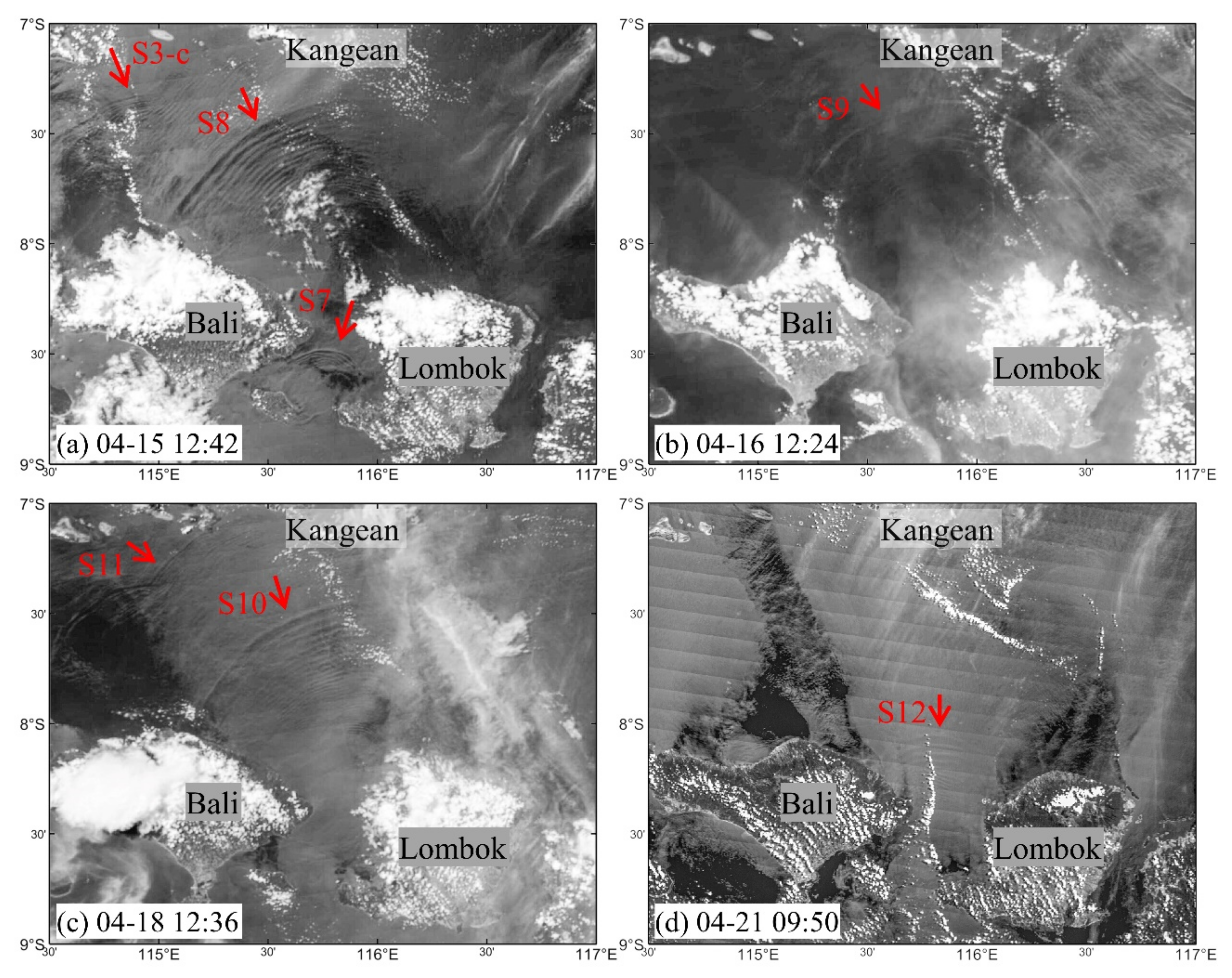
Up to three multi-wave ISW packets appeared simultaneously in one satellite image. In the VIIRS image of 15 April (Figure 2a), three distinguishable wave packets (S7, 8 and 3-c) were distributed in the LS, the BS basin and the continental shelf to the west of Kangean Islands, respectively, occupying a large portion of the BS. Actually, in the majority of the satellite images presented in Figure 1 and Figure 2, two multi-wave ISW packets are easily seen, suggesting the prevailing solitary waves in the BS near the time of the submarine wreck.

The locations of all leading ISW crests in 10 remote sensing images were extracted and plotted together to exhibit the distribution of ISWs (coloured curves in Figure 3a). It can be seen that, near the time of the submarine wreck, ISWs generally propagated toward the northwest, and thus, the ISWs were concentrated in the area north of Bali Island where the submarine wreck occurred. However, in the SAR images collected by Karang et al. from 2006 to 2011 and Karang et al. from 2014 to 2015 [14,29], most of ISWs propagated northeastward after being emitted from the LS, and those waves were mainly distributed in the area to the north of the Lombok Island rather than the Bali Island. This phenomenon indicates that the spatial distribution of ISWs in the BS has significant temporal variability, which may be modulated by dynamic processes such as mesoscale eddies. As is clear to all, ISWs in the area to the north of Bali Island were extraordinarily active in April 2021, which significantly increased the likelihood that submarines would encounter internal waves.

3.2. Propagation Speed of ISWs

Two MODIS images were available on 12, 14 and 19 April (Figure 1), and the 175-min interval of imaging time makes it possible to accurately calculate the propagation speed of ISWs (Figure 3c).

In the LS, a clear ISW packet (S3) was observed from the MODIS images on 14 April (Figure 1c,d). Within 175 min, the leading part of the wave center propagated northward for ~27 km, and the average speed was calculated to be 2.54 m/s accordingly. This value is very close to the ISW speed of 2.5 m/s obtained by Lindsey et al. [30] with a shorter 10-min time steps. Moreover, based on the assumption that the time interval of ISW generation in the LS is consistent with the tidal cycle, Susanto et al. [17] estimated the speeds of northward-propagating ISWs from the Lombok Strait as 1.97 and 1.96 m/s using ERS-1/2 SAR images of 23 and 24 April 1996 and Karang et al. [29] obtained a speed of 2.05 m/s using Landsat 8 image of 17 May 2015. It can be seen that the speed of ISW in the LS is not the same at different periods, and here we show a variation range of about 0.5 m/s.

In the BS basin, there are three observed ISWs (S1, 4 and 5) whose speeds decreased from south to north along the propagation path. The images on 19 April (Figure 1e,f) showed that the wave crest center of S5 moved at a mean speed of 2.69 m/s between 7.80° S and 7.57° S where the average water depth was 1274 m, and further to the northwest of the basin, the images on 12 April (Figure 1a,b) suggested that the wave crest center of S1 propagated at a mean speed of 2.24 m/s between 7.59° S and 7.40° S. Over the shallow terrain west of the Kangean Islands, the propagation speed of S6 severely slowed down to a mean value of 0.71 m/s in the area with an average water depth of 155 m. The above calculations show a clear decreasing trend of propagation speed as ISWs shoaled from the deep basin of the BS onto the continental shelf. Through numerical simulation, Ningsih et al. [22] showed an ISW propagation speed range in the BS of 0.71–2.67 m/s, especially consistent with our estimated result. Using ALOS PALSAR images, Matthews et al. [21] defined ISW mean speeds between two wave packets about 1.6 to 2.3 m/s by measuring the distances between the leading signals in adjacent wave packets generated 12.4 h apart.

Figure 2a shows that S3 reached the continental shelf to the west of the Kangean Islands at 12:42 on April 15. Compared with the images taken on 14 April (Figure 1c,d), it took more than a day for the wave to travel from the LS to the continental shelf. During the over 27-h process from formation to shoaling in shallow water, the ISW traveled nearly 200 km and the average propagation speed was about 2 m/s.

3.3. Underwater Structure of ISWs Inferred from MODIS Images

Understanding the underwater structure of ISWs near the wreck site is crucial for evaluating the impacts of ISWs on submarine navigation. About two days before the submarine disaster, a clear wave packet (S5-b) near the wreck site was captured by the MODIS at 12:55 on 19 April (Figure 1f), and its underwater structure was reconstructed here.

According to the MODIS image, the center of the leading wave of S5 propagated in a northwest direction with a half-wavelength of ~2 km at a depth of about 1200 m (Figure 4a), and its amplitude was inversed to be 41 m. Furthermore, the theoretical propagation speed $C$ of this ISW can be acquired by $C=C_0+\alpha {\eta }_0/3$. In this case, $C_0$ and $\alpha$ are 2.51 m/s and −0.0166 respectively, and the calculated $C$ is 2.73 m/s, which is in good agreement with the mean propagation obtained from the satellite images in Figure 1e,f.

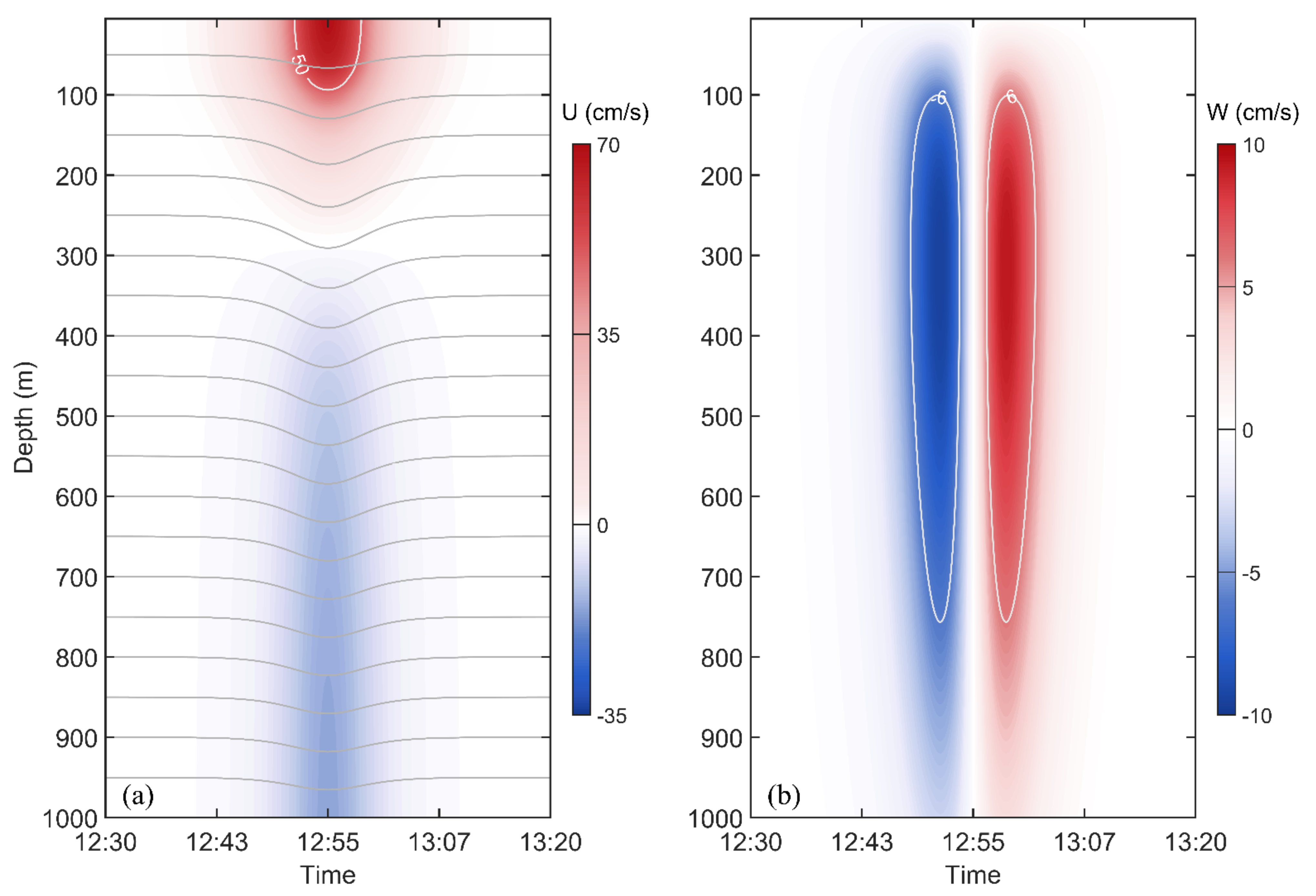
Figure 5 shows the underwater structure of the wave S5-b. As shown in the figure, the maximum horizontal current velocity induced by the wave was 65 cm/s, and the flow core with a velocity greater than 50 cm/s existed in the upper 50 m and spent nearly 10 min passing by the site where the ISW crest located. Below 300 m, the horizontal current direction of the ISW was opposite to the wave propagation direction. Vertically, there were downward and upward currents respectively before and after the wave trough with a maximum velocity of 10 cm/s, and the vertical flow exceeding 6 cm/s extended for 800 m and 650 m in the horizontal and vertical directions, respectively.

3.4. Relationship between Barotropic Tides at Source and ISWs

It is generally believed that ISWs in the LS are generated by the interaction between tidal current and the Nusa Penida sill [17,23,31]. Understanding the relationship between the ISW generation and barotropic tides is of great significance for estimating the occurrence time of ISWs in the BS around the time of submarine wreck.

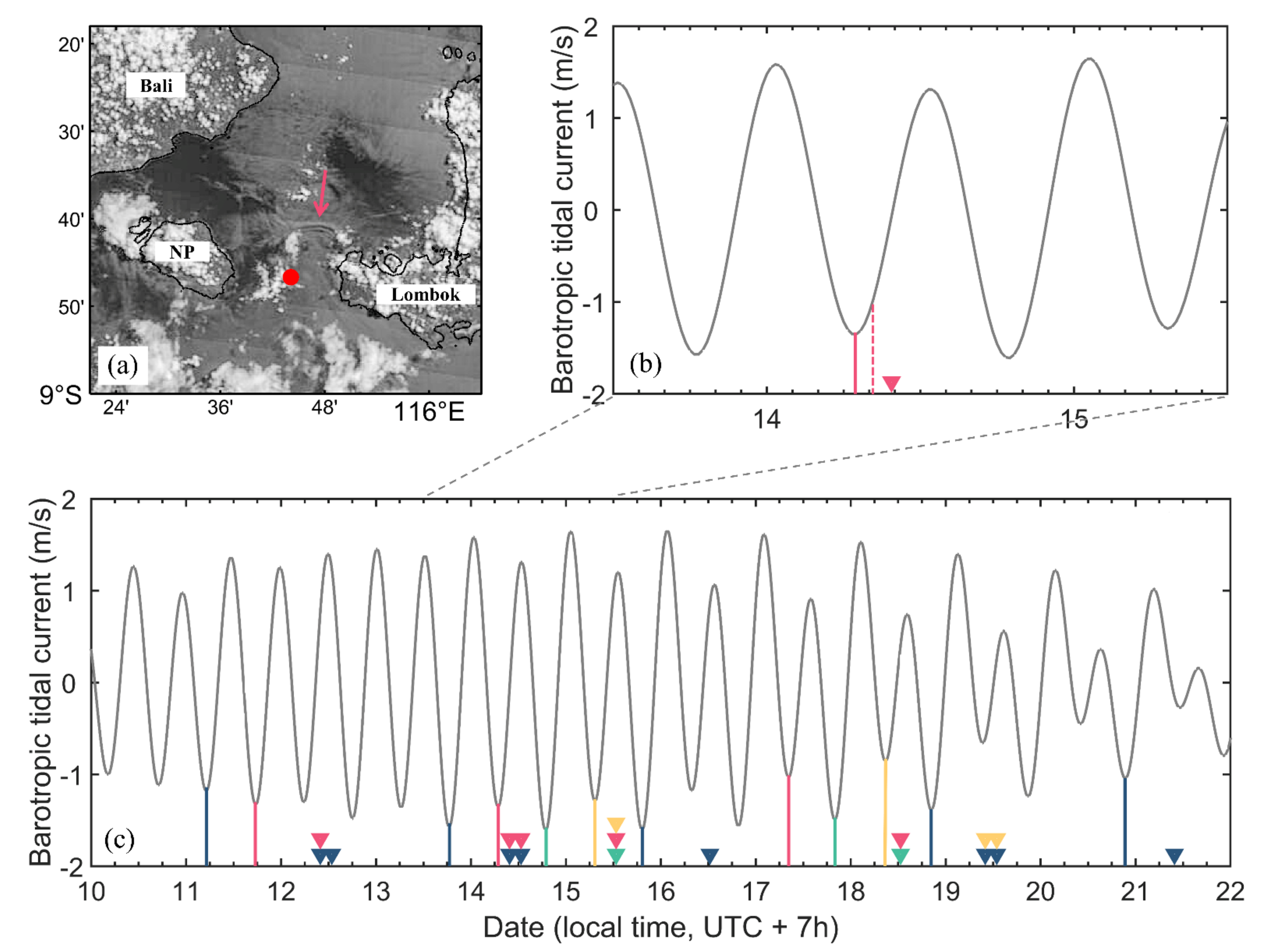
In the MODIS image taken at 9:45 on 14 April, it can be seen that the crest of S3-a was only about 10 km to the north of the source site (Figure 6a). Moreover, we calculated the internal Froude number (Fr) to examine the criticality of the tidal flow over the Nusa Penida sill. The Froude number (Fr = u/c) is a dimensionless quantity that expresses the ratio of barotropic flow speed (u) to the phase speed (c) of long internal wave [32]. At the above tidal peak, the Fr over the sill is 1.25 greater than 1, from which we can infer that S3 was likely released within the southward tidal. Backtracking at an average $C_0$ of 1.8 m/s, calculated from Equation (2), the generation time of S3 at the source site was about 08:12 (dashed red line in Figure 6b), adjacent to a TPXO southward tidal current peak. Purwandana et al. proposed that the generation of ISWs in the LS was related to the lee-wave mechanism [19], consistent with the near-source emergence of ISWs in the MODIS image in Figure 6a and the estimated release time of ISWs around the southward tidal current peak in Figure 6b.

As previous measurements have revealed [19], the barotropic tidal current at the Nusa Penida sill was dominated by semi-diurnal component, and every day there were two southward barotropic tidal current peaks, occurring about 20–30 min later than the barotropic tides each day (Figure 6c). This indicates that two ISWs were generated in one day over the April tidal period. We traceback each ISW along the propagation path using the speed obtained from the satellite images and the calculated theoretical speed, and connect these ISWs, in Figure 6c and

Table 1. The observed time of ISWs in satellite images from 12 to 21 April 2021 and the occurrence time of southward tidal current peaks (STCP) associated with their generation.

ISW	Observed Time	STCP Time	ISW	Observed Time	STCP Time
S1	04–12 09:55 04–12 12:50	04–11 05:10	S7	04–15 12:42	04–15 07:20
S2	04–12 09:55	04–11 17:30	S8	04–15 12:42	04–14 19:00
S3	04–14 09:45 04–14 12:40 04–15 12:42	04–14 07:00	S9	04–16 12:24	04–15 09:20
S4	04–14 09:45 04–14 12:40	04–13 18:30	S10	04–18 12:36	04–17 20:00
S5	04–19 10:00 04–19 12:55	04–18 20:20	S11	04–18 12:36	04–17 08:20
S6	04–19 10:00 04–19 12:55	04–18 08:40	S12	04–21 19:50	04–20 21:20

, with the suspected tidal peaks that generated them. From 11–20 April, the interval between the generation of two ISWs every day was reduced from 12.3 h to 11.7 h, slightly less than the 12.4 and the 12.42 h intervals defined by Matthews et al. and Karang et al. [21,29]. In addition, by comparing the distance between adjacent ISW crests and the time interval between their formation, we obtain a mean speed range of 1.35 (S1-a, S2) to 2.77 (S7, S8) m/s for the ISWs propagating in the BS.

4. Conclusions

By surveying remote sensing images over the BS, we found significant ISW activities near the submarine KRI nanggala-402 wreck site in April 2021. Those ISWs were generated in the LS and then traveled along the north-western direction in the BS basin, passing through the submarine wreck site, and finally reached the continental shelf to the west of the Kangean Islands. The ISWs in April 2021 were mainly distributed in the area to the north of Bali Island, rather than north of Lombok Island as was revealed by previous studies, indicating a significant temporal variation of ISW distribution in the BS.

Along the propagation path, there were up to three wave packets simultaneously existing in the BS. The wave packet contained dozens of solitons, whose crest can extend for 200 km, within a meridional range of more than 60 km, covering a vast region of the BS. Those ISWs propagated at a mean speed of 2 m/s from the source region to the continental shelf, and the speed was as fast as 2.69 m/s in the BS basin and reduced to 0.71 m/s in the shallow water. On 19 April, about two days before the submarine incident, the amplitude of an ISW near the submarine wreck site was inversed to be 41 m according to satellite images, and the reconstructed underwater structure showed a maximum horizontal and vertical velocity of 65 cm/s and 10 cm/s, respectively. Moreover, it was inferred from the near-source evidence that ISWs were released within the southward barotropic tidal trough, and the variation of source tides revealed that two ISWs were generated with an interval of 11.7 to 12.3 h every day during the April tidal period.

The analyses presented here have provided necessary observational information on the ISW activities in the BS for the submarine wreck investigations, and whether or not the submarine KRI nanggala-402 encountered with ISWs will be ascertained once the accurate time and location site of the submarine wreck becomes available in the future. In addition, it seemed that ISWs in the area to the north of Bali Island were extraordinarily active around the time of the submarine wreck in comparison with the statistical results from 2006 to 2011 and from 2014 to 2015 based on satellite images [14,29]. Such variability of ISW distribution is also an interesting topic worth further investigation, and long in-situ observations prove the necessary to improve the understanding of the ISWs in BS.

References

- Alford, M.H.; Mickett, J.B.; Zhang, S.; MacCready, P.; Zhao, Z.; Newton, J. Internal Waves on the Washington Continental Shelf. Oceanography 2012, 25, 66–79. [Google Scholar] [CrossRef]
- Da Silva, J.C.B.; New, A.L.; Srokosz, M.A.; Smyth, T. On the observability of internal tidal waves in remotely-sensed ocean colour data. Geophys. Res. Lett. 2002, 29, 10-1–10-4. [Google Scholar] [CrossRef]
- Huang, X.; Wang, Z.; Zhang, Z.; Yang, Y.; Zhou, C.; Yang, Q.; Zhao, W.; Tian, J. Role of Mesoscale Eddies in Modulating the Semidiurnal Internal Tide: Observation Results in the Northern South China Sea. J. Phys. Oceanogr. 2018, 48, 1749–1770. [Google Scholar] [CrossRef]
- Huang, X.; Zhang, Z.; Zhang, X.; Qian, H.; Zhao, W.; Tian, J. Impacts of a Mesoscale Eddy Pair on Internal Solitary Waves in the Northern South China Sea revealed by Mooring Array Observations. J. Phys. Oceanogr. 2017, 47, 1539–1554. [Google Scholar] [CrossRef]
- Kinder, T.H. Net mass transport by internal waves near the Strait of Gibraltar. Geophys. Res. Lett. 1984, 11, 987–990. [Google Scholar] [CrossRef]
- Raju, N.J.; Dash, M.K.; Dey, S.P.; Bhaskaran, P.K. Potential generation sites of internal solitary waves and their propagation characteristics in the Andaman Sea—a study based on MODIS true-colour and SAR observations. Environ. Monit. Assess. 2019, 191, 809. [Google Scholar] [CrossRef] [PubMed]
- Ramp, S.; Tang, T.Y.; Duda, T.; Lynch, J.; Liu, A.; Chiu, C.-S.; Bahr, F.; Kim, H.-R.; Yang, Y.-J. Internal Solitons in the Northeastern South China Sea Part I: Sources and Deep Water Propagation. IEEE J. Ocean. Eng. 2004, 29, 1157–1181. [Google Scholar] [CrossRef]
- Zhang, X.; Huang, X.; Zhang, Z.; Zhou, C.; Tian, J.; Zhao, W. Polarity Variations of Internal Solitary Waves over the Continental Shelf of the Northern South China Sea: Impacts of Seasonal Stratification, Mesoscale Eddies, and Internal Tides. J. Phys. Oceanogr. 2018, 48, 1349–1365. [Google Scholar] [CrossRef]
- Huang, X.; Chen, Z.; Zhao, W.; Zhang, Z.; Zhou, C.; Yang, Q.; Tian, J. An extreme internal solitary wave event observed in the northern South China Sea. Sci. Rep. 2016, 6, 30041. [Google Scholar] [CrossRef] [Green Version]
- Osborne, A.; Burch, T.; Scarlet, R. The Influence of Internal Waves on Deep-Water Drilling. J. Pet. Technol. 1978, 30, 1497–1504. [Google Scholar] [CrossRef]
- Chen, J.; You, Y.X.; Liu, X.D.; Wu, C.S. Numerical simulation of interaction of internal solitary waves with a moving submarine. J. Hydrodyn. 2010, 25, 344–351. (In Chinese) [Google Scholar]
- Huang, M.M.; Zhang, N.; Zhu, A.J. Hydrodynamic loads and motion features of a submarine with interaction of internal solitary waves. J. Ship Mech. 2019, 23, 531–540. (In Chinese) [Google Scholar]
- Stepanyants, Y. How internal waves could lead to wreck American and Indonesian submarines? arXiv 2021, arXiv:2107.00828. [Google Scholar]
- Karang, I.W.G.A.; Nishio, F.; Mitnik, L.; Osawa, T. Spatial-Temporal Distribution and Characteristics of Internal Waves in the Lombok Strait Area Studied by Alos-Palsar Images. Earth Sci. Res. 2012, 1, 11. [Google Scholar] [CrossRef]
- Matthews, J.; Awaji, T. Synoptic mapping of internal-wave motions and surface currents near the Lombok Strait using the Along-Track Stereo Sun Glitter technique. Remote Sens. Environ. 2010, 114, 1765–1776. [Google Scholar] [CrossRef]
- Mitnik, L.; Alpers, W.; Chen, K.S.; Chen, A.J. Manifestation of internal solitary waves on ERS SAR and SPOT images: Similarities and differences. In Proceedings of the IGARSS 2000. IEEE 2000 International Geoscience and Remote Sensing Symposium. Taking the Pulse of the Planet: The Role of Remote Sensing in Managing the Environment, Honolulu, HI, USA, 24–28 July 2000; Volume 5, pp. 1857–1859. [Google Scholar] [CrossRef]
- Susanto, R.D.; Mitnik, L.; Zheng, Q. Ocean Internal Waves Observed in the Lombok Strait. Oceanography 2005, 18, 80–87. [Google Scholar] [CrossRef]
- Syamsudin, F.; Taniguchi, N.; Zhang, C.; Hanifa, A.D.; Li, G.; Chen, M.; Mutsuda, H.; Zhu, Z.; Zhu, X.; Nagai, T.; et al. Observing Internal Solitary Waves in the Lombok Strait by Coastal Acoustic Tomography. Geophys. Res. Lett. 2019, 46, 10475–10483. [Google Scholar] [CrossRef] [Green Version]
- Purwandana, A.; Cuypers, Y.; Bouruet-Aubertot, P. Observation of internal tides, nonlinear internal waves and mixing in the Lombok Strait, Indonesia. Cont. Shelf Res. 2021, 216, 104358. [Google Scholar] [CrossRef]
- Aiki, H.; Matthews, J.P.; Lamb, K.G. Modeling and energetics of tidally generated wave trains in the Lombok Strait: Impact of the Indonesian Throughflow. J. Geophys. Res. Earth Surf. 2011, 116, C03023. [Google Scholar] [CrossRef] [Green Version]
- Matthews, J.P.; Aiki, H.; Masuda, S.; Awaji, T.; Ishikawa, Y. Monsoon regulation of Lombok Strait internal waves. J. Geophys. Res. Earth Surf. 2011, 116, C05007. [Google Scholar] [CrossRef]
- Ningsih, N.S.; Rachmayani, R.; Hadi, S.; Brodjonegoro, I.S. Internal Waves Dynamics in The Lombok Strait Studied By A Numerical Model. Int. J. Remote Sens. Earth Sci. 2010, 5, 17–33. [Google Scholar] [CrossRef] [Green Version]
- Mitnik, L.; Alpers, W.; Lim, H. Thermal plumes and internal solitary waves generated in the Lombok Strait studied by ERS SAR. In Proceedings of the ERS-Envisat Symposium: Looking down to Earth in the New Millennium, Gothenburg, Sweden, 16–20 October 2000. [Google Scholar]
- Zhao, Z.X.; Klemas, V.V.; Zheng, Q.N.; Yan, X.H. Satellite observation of internal solitary waves converting polarity. Geophys. Res. Lett. 2003, 30, 1988. [Google Scholar] [CrossRef]
- Jackson, C. Internal wave detection using the Moderate Resolution Imaging Spectroradiometer (MODIS). J. Geophys. Res. Earth Surf. 2007, 112, C11012. [Google Scholar] [CrossRef] [Green Version]
- Huang, X.D.; Zhao, W. Information of Internal Solitary Wave Extracted from MODIS image: A Case in the Deep Water of Northern South China Sea. Period. Ocean. Univ. China 2014, 44, 19–23. [Google Scholar]
- Ning, J.; Wang, J.; Zhang, M.; Cui, H.J.; Lu, K.X. Amplitude Inversion Model and Application of Internal Solitary Waves of the Northern South China Sea Based on Optical Remote-sensing Images. ACTA Photonica Sinica 2019, 48, 1228003. (In Chinese) [Google Scholar] [CrossRef]
- Zheng, Q.; Yuan, Y.; Klemas, V.; Yan, X.-H. Theoretical expression for an ocean internal soliton synthetic aperture radar image and determination of the soliton characteristic half width. J. Geophys. Res. Earth Surf. 2001, 106, 31415–31423. [Google Scholar] [CrossRef]
- Karang, I.W.G.A.; Chonnaniyah, C.; Osawa, T. Landsat 8 Observation of the Internal Solitary Waves in the Lombok Strait. Indones. J. Geogr. 2019, 51, 251–260. [Google Scholar] [CrossRef] [Green Version]
- Lindsey, D.T.; Nam, S.; Miller, S.D. Tracking oceanic nonlinear internal waves in the Indonesian seas from geostationary orbit. Remote Sens. Environ. 2018, 208, 202–209. [Google Scholar] [CrossRef]
- Mitnik, L.; Alpers, W. Sea surface circulation through the Lombok Strait studied by ERS SAR. In Proceedings of the 5th Pacific Ocean Remote Sensing Conference (PORSEC 2000), Goa, India, 5–8 December 2000; Volume I, pp. 313–317. [Google Scholar]
- Farmer, D.M.; Smith, J.D. Tidal interaction of stratified flow with a sill in Knight Inlet. Deep Sea Res. Part A Oceanogr. Res. Pap. 1980, 27, 239–254. [Google Scholar] [CrossRef]