Article

A Hybrid Model Based on the Bifurcation Approach for Internal Turbulent Flow with Rotation and Streamline Curvature Effects

1
College of Electrical, Energy and Power Engineering, Yangzhou University, Yangzhou 225009, China
2
School of Water Conservancy and Civil Engineering, Northeast Agricultural University, Harbin 150030, China
3
College of Water Resources and Civil Engineering, China Agricultural University, Beijing 100083, China
4
Beijing Engineering Research Center of Safety and Energy Saving Technology for Water Supply Network System, Beijing 100083, China
*
Author to whom correspondence should be addressed.
J. Mar. Sci. Eng. 2022, 10(12), 2022; https://doi.org/10.3390/jmse10122022
Submission received: 17 November 2022 / Revised: 12 December 2022 / Accepted: 14 December 2022 / Published: 18 December 2022

Abstract

:
This study aims to research the prediction performance of a bifurcated adaptive DDES (BADDES) model in different turbulent flows with rotation and curvature. The k ω model is modified by the bifurcation approach to account for the rotation and streamline curvature effects and then used as a base model to establish the BADDES model. The BADDES model was tested in rotating channel flow, Taylor-Couette flow, and swirling flow through an abrupt axisymmetric expansion. The velocity distribution of the BADDES model is slightly superior to that of other models. Additionally, the BADDES model is superior to other models at predicting RMS velocity. In addition, the URANS region of the BADDES model is thinner, meaning that the BADDES model can switch from the URANS model to the eddy simulation branch faster. The BADDES model can capture smaller-scale vortex structures than other models.

1. Introduction

Water jet propulsion pumps are among the most critical facilities for modern ships affording the required power. Many studies [1,2,3,4,5,6] have focused on the internal field of the pump using CFD to improve the design or reveal the mechanisms involved. Rotating turbulence is the key characteristic of the pump. It has a high adverse pressure gradient, large streamline curvature, and strong rotation effect, making it challenging to predict the flow structure accurately. The Reynolds averaged Navier–Stokes (RANS) model is not sensitive to capturing the rotation and streamlined curvature effects due to its native defects [7,8]. Meanwhile, due to the high computation cost, it is hard to use direct numerical simulation (DNS) or large eddy simulation (LES) to simulate a rotating machine with a high Reynolds number. Therefore, it is more suitable to incorporate the effects of rotation and streamlined curvature into the hybrid turbulence model, which couples RANS with LES [9].
Detached eddy simulation (DES), which was proposed by Spalart et al. [10], is a seamless hybrid method that couples unsteady RANS (URANS) models and eddy-resolving simulations [11]. Shielding functions are used to solve the modeled stress depletion (MSD) problem [12,13], which can switch from the URANS to the LES outside the boundary layer. The resulting model was named delayed DES (DDES). There are also some drawbacks to the DDES, such as log-layer mismatch (LLM) [14] and slow large-eddy simulation development in mixing layers (SLD) [15]. LLM can be alleviated by modifying the shielding function [14,16] or length scale definition [17]. SLD can be alleviated by modifying the Smagorinsky model (SM) of the eddy branch of a DDES [18]. The modification measures include alternating the grid scale [17,19,20,21], replacing the SM model with the WALE model or σ model [20], or dynamically calculating the model coefficients [9,22,23,24,25,26]. Reddy et al. [17] proposed the l 2 ω DDES model, which could alleviate both the LLM and SLD. Yin et al. [9] implemented the dynamic procedure for computing the coefficient of the l 2 ω DDES. An inferior bound was added to gauge the mesh resolution and prohibit the invocation of the dynamic procedure on a coarse grid, and this method was named adaptive DDES (ADDES) [22]. According to previous studies, ADDES has apparent advantages in the DES series.
As a relatively new method, ADDES has seen limited applications in rotating machinery. However, we can see the prospects of this method from the application of DDES [15,18,24,26,27,28,29,30,31,32,33,34,35]. There are two drawbacks to the ADDES model: (1) The ADDES model does not systematically account for the system rotation and streamline curvature effects, resulting in less-than-ideal results for the rotating channel flow [31] and rotating machinery [32,33,34,35]. (2) There is still a retained near-wall URANS region, even when the mesh is fine enough to resolve the LES [22,23,24]. Thus, the system rotation and streamline curvature effects should be included in the ADDES model. Moreover, the transition between URANS and LES should be carefully considered. Therefore, the motivation of the present work is to solve these two deficiencies in the ADDES model.
In order to deal with the first drawback, we should first incorporate the effects of rotation and streamlined curvature into the URANS turbulence model. There are three methods to sensitize the linear eddy viscosity models to rotation and streamline curvature: the “non-linear approach [36,37,38,39]”, the “modified coefficients approach [40,41,42]”, and the “bifurcation approach [43,44,45]”. The principal idea of the bifurcation approach is to mimic the behavior of a second-moment closures (SMC) model in incompressible rotating homogeneous shear flow. Many scholars have verified that the prediction results of the bifurcation approach are more accurate than those of other approaches [7,8,44,45,46,47,48]. In order to deal with the second drawback, improving the ability to resolve the flow field of the URANS model is a new idea to alleviate the SLD problem. According to several scholars [43,46,47,48], another significant advantage of the bifurcation approach is that the resolution of the velocity fluctuation of the flow field is accurate. Therefore, the basic idea of the present work is to use the URANS model modified by the bifurcation approach to build a new adaptive DDES model that solves the two deficiencies of the ADDES model.
In the present work, the rotation and streamline curvature effects are introduced to the k ω model by the bifurcation approach and are then used as a background model to establish a new adaptive DDES method. Then, we compare the prediction effects by simulating three flows with different rotation and curvature effects: rotating channel flow, Taylor-Couette flow, and swirling flow through an abrupt axisymmetric expansion.

2. Model Formulation

In the present work, we compared four different turbulence models, all of which are based on the k ω model. The model formulation of the original Wilcox k ω model [49] and the four different turbulence models are briefly introduced in this chapter. Section 2.2 introduces the bifurcation k ω model proposed in our previous work [48], which is a RANS model and considers the effects of rotation and curvature. Section 2.4 introduces the modified k ω model using the shielding function of the original DDES method, which is a hybrid k ω and LES model. Section 2.5 presents the existing adaptive DDES model. Section 2.6 introduces the main innovation of this paper. We modified the adaptive DDES model based on the bifurcation model. All four models were self-realized on the open-source code OpenFOAM-2.4.0.

2.1. The Original Wilcox k ω Model

The Wilcox k ω model [49] is of the form:
k t + u j k x j = 2 ν t | S | 2 C μ k ω + x j ( ( ν + σ k ν T ) k x j ) ,
ω t + u j ω x j = 2 C ω 1 | S | 2 C ω 2 ω 2 + x j ( ( ν + σ ω ν T ) ω x j ) ,
where ν t = k / ω . The standard constants are invoked, i.e., C ω 1 = 5 / 9 , C ω 2 = 3 / 40 , C μ = 0.09 , σ k = 0.5 , σ ω = 0.5 .

2.2. The Modified Bifurcation k ω Model (Named the BkO Model) (RANS Model)

In the incompressible homogeneous shear flow, as in the k ω model, the k and ω equation of the model can be simplified to:
d k d t = C μ k ω S 2 C μ k ω ,
d ω d t = C ω 1 S 2 C ω 2 ω 2 = C ω 1 v t P k C ω 2 ω 2 ,
where ν t = C μ k / ω and C μ * = 1 . The dissipation rate ε = C μ k ω is inserted. Then, Equations (3) and (4) can be combined to give the following:
d d ( S t ) ( ε S k ) = ( ε S k ) 2 [ ( C ε 1 1 ) P ε ( C ε 2 1 ) ] .
Two equilibria of Equation (5) are obtained by setting d S t ( ε / S k ) = 0 . Therefore, there are two branches. The first branch ( ε / S k ) 0 represents when the turbulent kinetic energy increases exponentially with time; the second branch ( ε / S k ) = 0 represents when the evolution of turbulent kinetic energy with time is in the form of a power law.
The specific coefficient derivation process and the constraints that should be satisfied can be found in the literature [43]. The final form of the bifurcation k ω model can be written as:
C μ = C μ ( 1 + α ω 5 η 1 1 + α ω 5 η 2 + α ω 1 η 2 | η 3 | η 3 ) 1 1 + α ω 2 | η 3 | + α ω 3 η 3 1 + α ω 4 | η 3 | .
The model coefficients are given by ( α ω 1 , α ω 2 , α ω 3 , α ω 4 , α ω 5 ) = ( 0.062 , 0.8 , 0.4 , 0.4 , 0.025 ) . The bifurcation point is the same as the k ε model, and the restabilization point is at | | = 1.62 , corresponding to Ω F / S = ( + 1.16 , 0.28 ) .

2.3. Unification of Rotation and Curvature

Rotation and curvature are analogous, and they can be unified using the Spalart–Shur tensor [44,46]. The rate of rotation is given by:
Ω i j mod = Ω i j * + ( C r 1 ) W i j A .
The Spalart–Shur tensor is an antisymmetric tensor that is defined in terms of the convective derivative of the strain rate tensor:
Ω S S Ω F S . D t S D t S . S 2 | S | 2 .
In 2D, W j k A = Ω j k S S . In 3D, this is a change to W j k A = Ω j k F ϵ i j k w i in which
w i = I I S X i j ( Ω p q F ϵ p q j Ω r s S S ϵ r s j ) ,
X i j = I I S 2 δ i j + 12 I I I S S i j + 6 I I S S i k S k j 2 I I S 3 12 I I I S 2
where I I S = S i j S j i and I I I S = S i j S j k S k i . The rate of rotation tensor invariant used in the model is: η 2 m o d = Ω i j m o d Ω i j m o d .

2.4. The Modified DDES Model Based on the k ω Model (Named the DDESO Model) (Hybrid k ω with the LES Model)

The governing equations of the DDESO model read as:
k t + u j k x j = 2 ν t | S | 2 k 3 / l D D E S + ( ( ν + σ k ν T ) k ) ,
ω t + u j ω x j = 2 C ω 1 | S | 2 C ω 2 ω 2 + ( ( ν + σ ω ν T ) ω )
The DDESO length scale in Equation (11) reads as follows:
l D D E S = l R A N S f d max ( 0 , l R A N S l L E S ) , l R A N S = k / C μ ω , l L E S = C D E S Δ ,
where C D E S = 0.12 is the model coefficients, and the grid spacing Δ is proposed by Reddy et al. [17]:
Δ = f d V 1 / 3 + ( 1 f d ) h max ,
where V is the cell volume, h max = max ( d x , d y , d z ) is the maximum cell spacing among the three directions, and f d is the DDES shielding function proposed by Sparlat et al. [12]:
f d = 1 tanh ( [ 8 r d ] 3 ) , r d = k / ω + ν κ 2 d ω 2 U i , j U i , j ,
where ν is the kinematic viscosity, κ is the Von Kármán constant, d w is the wall distance, and U i , j is the velocity gradient tensor.

2.5. The Adaptive DDES Model (Named the ADDES Model)

The ADDES model [9] takes the form:
k t + u j k x j = 2 l A D D E S 2 ω | S | 2 C μ k ω + ( ( ν + σ k ν T ) k ) ,
ω t + u j ω x j = 2 C ω 1 | S | 2 C ω 2 ω 2 + ( ( ν + σ ω ν T ) ω ) .
The standard constants used are the same as in Section 2.1. The ADDES length scale in Equation (16) reads as follows:
l A D D E S = l R A N S _ A f d max ( 0 , l R A N S _ A l L E S ) , l R A N S _ A = k / ω , l L E S = C D E S Δ .
The same grid spacing Δ and shielding function f d is used in the ADDES. Then, ν t = l D D E S 2 ω is used to define the production term of the k equation in the k ω model, leaving all the other terms unaltered. Therefore, on the URANS branch ( f d = 0 , l L E S > l R A N S ), we have
ν t = ( k / ω ) 2 ω = k / ω ,
the same as the k ω model. On the eddy simulation branch ( f d = 1 , l L E S < l R A N S ),
ν t = ( C D E S Δ ) 2 ω ,
which is similar to the sub-grid viscosity expression of SM:
ν t = ( C D E S Δ ) 2 ω .
Lilly proposed a dynamic procedure in LES to evaluate the model constant C S . Indeed, ω plays a similar role to the filtered rate of the strain | S | away from the near-wall region. Therefore, Yin et al. [9] applied the dynamic procedure of DSM to evaluate C D E S . The usual rationale is that scale similarity allows for resolved fluctuations to be used to estimate the sub-grid stresses. We define the test filter stresses as:
M i j = ( Δ 2 ω S i j ^ Δ ^ 2 ω ^ S ^ i j ) ,
L i j = u i u j ^ u i ^ u j ^ .
Though the C D E S could be computed using Equations (22) and (23), a fine grid is required. To correctly evaluate C D E S , a lower bound is used to avoid the dynamic procedure on the coarse grid.
C d y n 2 = max ( 0 , 0.5 L i j M i j M i j M i j ) ,
C D E S = max ( C lim , C d y n ) ,
C lim = C D E S 0 [ 1 tanh ( α exp ( β h max η ) ) ] .
where C D E S 0 = 0.12 , α = 25 , β = 0.05 , and η = ( ν 3 / ε ) 1 / 4 .

2.6. The New Bifurcation Adaptive DDES Model (Named the BADDES)

Equations (3) and (16) show that both the bifurcation approach and adaptive DDES modify the production term of the k equation. Therefore, two constraints should be followed:
  • There is no conflict between the two methods for the correction of the production term in the k equation;
  • The bifurcation k ω model only acts on the URANS region inside the boundary layer.
Thus, the URANS length scale l R A N S _ B A should be modified to satisfy the two constraints.
l R A N S _ B A = C μ k / ω .
The new bifurcation adaptive DDES model is of the form:
k t + u j k x j = 2 l BADDES 2 ω | S | 2 C μ k ω + ( ( ν + σ k ν T ) k ) ,
ω t + u j ω x j = 2 C ω 1 | S | 2 C ω 2 ω 2 + ( ( ν + σ ω ν T ) ω ) .

3. Test Cases

Three standard test cases are simulated in this section to study the performance of the BADDES model in different turbulent flows: rotating channel flow with system rotation, Taylor-Couette flow with wall rotation and curvature effect, and swirling flow through abrupt axisymmetric expansion with inlet swirling flow. The present work compares the prediction results with the available experimental or DNS results. All cases were simulated using the open-source code OpenFOAM-2.4.0. The matrix system of pressure was solved using the pre-conditioned gradient (PCG) algorithm with the geometric-algebraic multi-grid (GAMG) preconditioner. Other asymmetric matrices were solved using smoothSolver with the GaussSedil smoother. Gaussian finite volume integration with the second-order Gauss linear scheme (central difference scheme) was used for the spatial discretization of equations for the first two cases. In addition, the second-order Gauss QUICK (quadratic upwind interpolation of convective kinematics) scheme was used to discrete the convection and diffusion terms to improve its convergence for the last case. The second-order backward difference scheme was used for time discretization. It should be noted that URANS equations retain the transient term.
In URANS, the usual Reynolds decomposition is employed as follows [50]:
v ¯ ( t ) = 1 2 T t T t + T v ( t ) d t , v = v ¯ + v + v
where v ¯ is the time-averaged velocity, v is the resolved fluctuation, and v is the modeled turbulent fluctuation. We should ensure that the turbulence model is not too dissipative so as not to kill the resolved fluctuations v [50]. Therefore, all results of the Reynolds stress in this study were v , the resolved fluctuation.

3.1. Rotating Channel Flow

3.1.1. Benchmark Description and Computational Setup

The first case is rotating channel flow, a flow type with system rotation. In this paper, we use the DNS data from the study by Yang et al. [51].
Figure 1 is a sketch of the rotating channel flow extracted from the literature [52]. The dimensions of the channel streamwise (x), in the normal direction (y), and spanwise (z) are 2 π h , 2 h , and 2 π h , respectively. The average velocity is U m , the Reynolds number is Re = U m h / ν = 7000 , h is the half channel height, and ν is the kinematic viscosity. The rotation number is R o = 2 ω h / U m = 0.3 , where ω is the rotational angular velocity.
The governing equation under the rotating reference system is used in the calculation:
u i x i = 0 ,
u i t + u j u i x j = 1 ρ p x i + ν 2 u i x j x j τ i j x j + F c o r + d P d x j .
F c o r = 2 ω × u represents the Coriolis body force, and ω is the rotational angular velocity vector. The centrifugal force in the rotating system is a scalar quantity and is included in the pressure term [52]. The pressure gradient drives the flow in the streamwise direction, and the pressure gradient in the normal and span directions is zero. A self-compiled channelRotate solver is used to solve the governing equation. The Pressure Implicit with the Splitting of Operator (PISO) algorithm is used to calculate the pressure–velocity coupling. In the calculation process, after each time step, an iterative calculation is completed to ensure that the Reynolds number is constant, and the solver will automatically adjust the velocity distribution of the inlet section. The flow and span direction of the rotating channel flow are set as periodic boundary conditions. The upper and lower walls are set as the non-slip wall boundary conditions. The grid number in the three directions is 48, 64, and 128, respectively. The streamwise and spanwise grids are uniformly distributed, and the normal direction is locally encrypted in the near-wall area, corresponding to y + 0.8 . This grid number is verified by Huang et al. [52] to be suitable for solving the rotating channel flow.
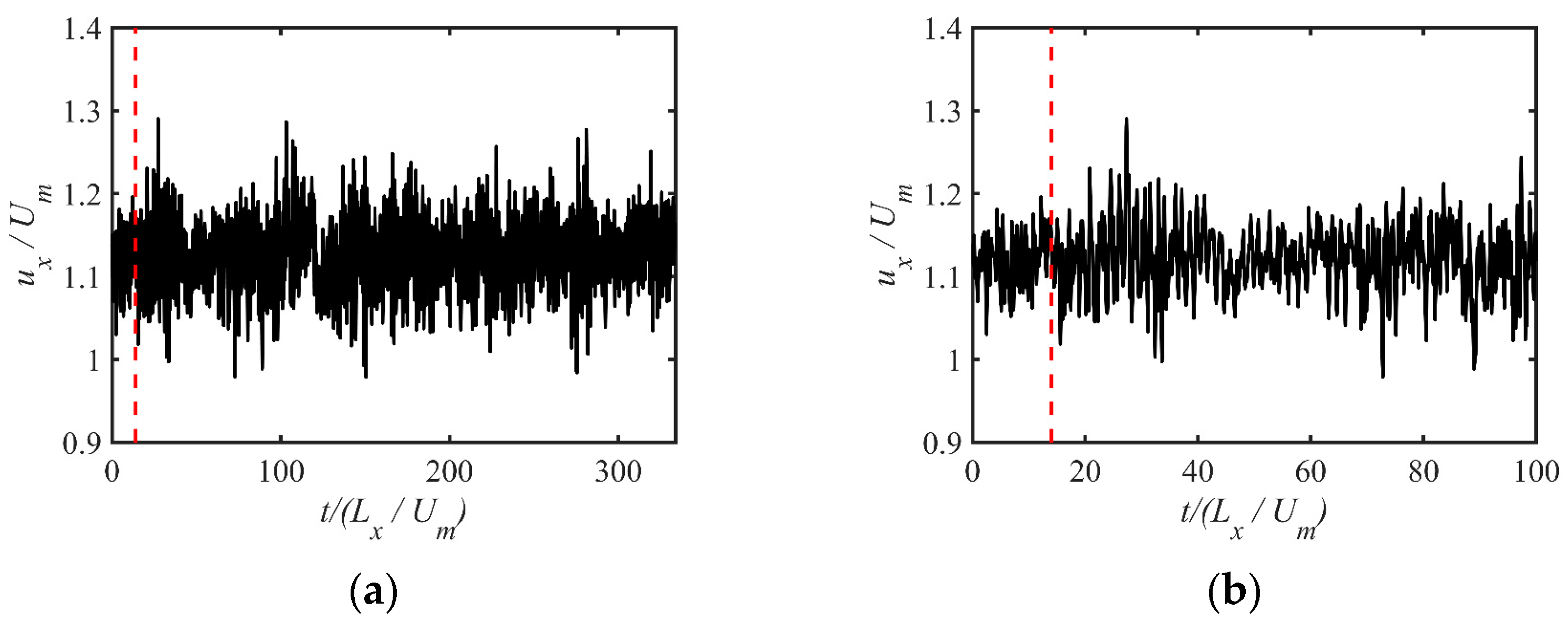
In the calculation process, the maximum Courant-Friedrichs-Lewy (CFL) number does not exceed 0.6. The initial velocity field with high and low-velocity intervals was generated by a method proposed by Eugene [53] to make the flow develop into a fully developed turbulent flow as soon as possible. Figure 2 shows that the change in the transient streamwise velocity with time at the center of the channel corresponds to the coordinates of (3.14, 1, 1) in the BADDES calculation results. The time is dimensionless with the flow cycle L x / U m . L x is the length of the channel. It can be seen that the calculation reaches a stable state after about 14 flow cycles. Therefore, the first 14 flow cycles were used to eliminate the transient characteristics of the flow, the last 306 cycles were averaged, and the whole simulation included a total of about 334 flow cycles.
In this case, all results are spanwise, streamwise, and time-averaged results to match the results of the DNS. The mean velocity u s is defined as:
u s = 1 L x L z T 0 L x 0 L z 0 T u ¯ s d x d z d t .
where u ¯ s is the transient streamwise velocity and L z is the spanwise length of the channel.

3.1.2. Results and Discussion

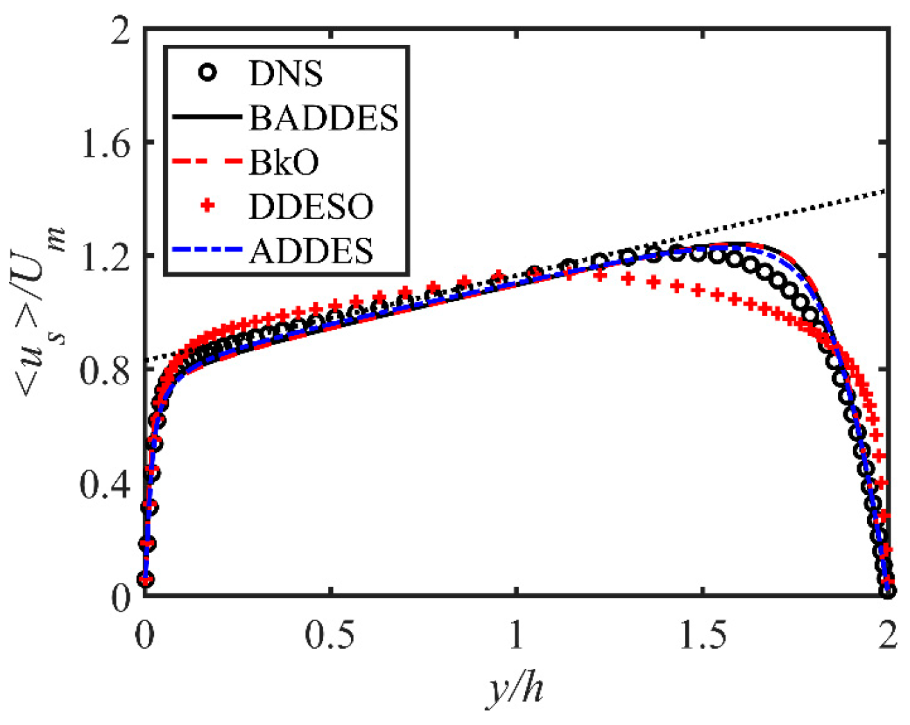
It should be pointed out that the “DNS” in the legend represents the result of the DNS, which is indicated by a black circle. “BADDES” in the legend represents the BADDES model, which is represented by solid black lines. “ADDES” in the legend represents the adaptive DDES model, which is represented by a blue dotted line. “BkO” in the legend represents the modified bifurcation k ω model, which is indicated by a red dotted line. “DDESO” in the legend represents the modified DDES model based on the k ω model, which is indicated by a red + sign.
Figure 3 shows the streamwise mean velocity distribution with different turbulence models. The DNS results show that the velocity gradually increases from the pressure side (y/h = 0) to the suction side (y/h = 2), indicating that rotation effects influence turbulence. The results of the BADDES model, ADDES model, and BkO model are very close, and all can capture the rotation effect. However, the DDESO model cannot predict the asymmetry velocity distribution, indicating that the original DDES method cannot make the base model capture the rotation effect.
Figure 4 shows the distribution of the root-mean-square (RMS) of the Reynolds stress components and the turbulent kinetic energy of the rotating channel flow with different turbulence models. It should be recalled that all results of the Reynolds stress are only the resolved part. The definition of turbulent kinetic energy is:
k u = 1 2 u i u i .
From the results, the value on the pressure side is greater than the value on the suction side, which shows that the rotation effect enhances the turbulence on the pressure side while suppressing the turbulence intensity on the suction side. This result is consistent with the results of other studies [1,2,36,37].
The BADDES and BkO model results are also very close and slightly superior to those of the ADDES model. However, there is an abnormally high value of the streamwise velocity fluctuation and turbulent kinetic energy of the BADDES model and BkO model near the pressure side, perhaps related to the numerical error. The results on the pressure side of the ADDES model are closer to those of DNS. In addition, the results of the BADDES, ADDES, and BkO models are far superior to those of the DDESO model.
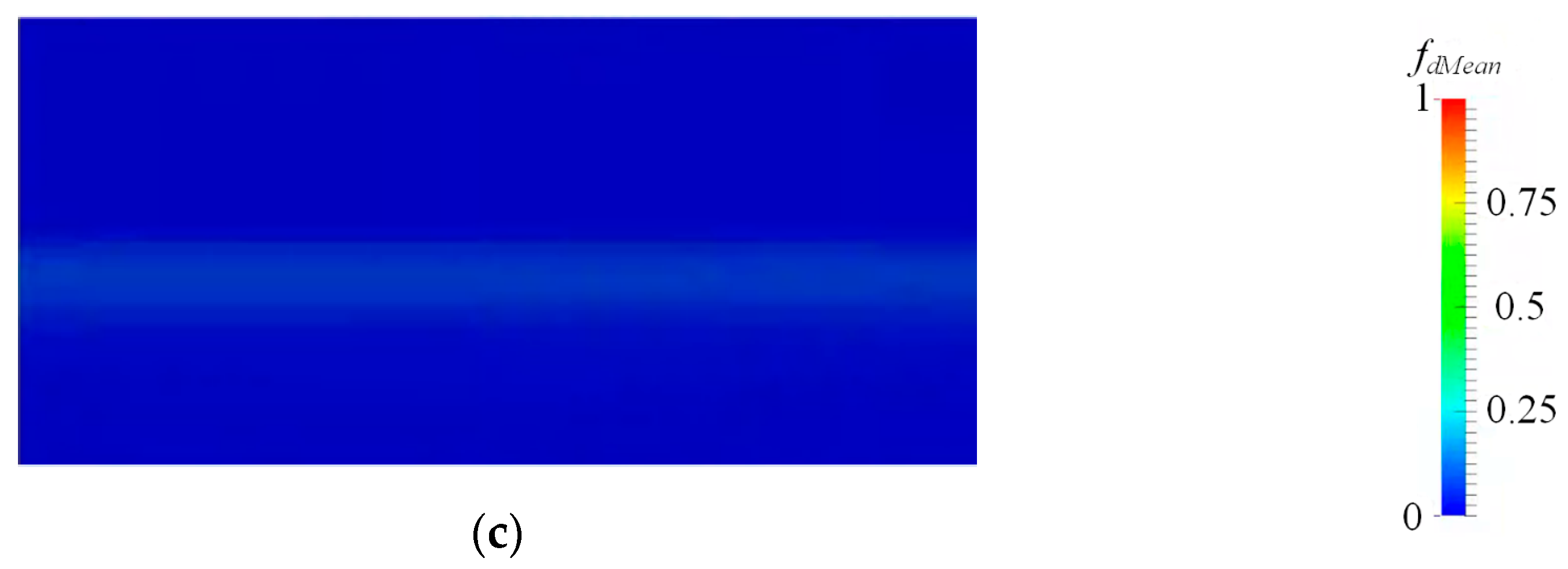
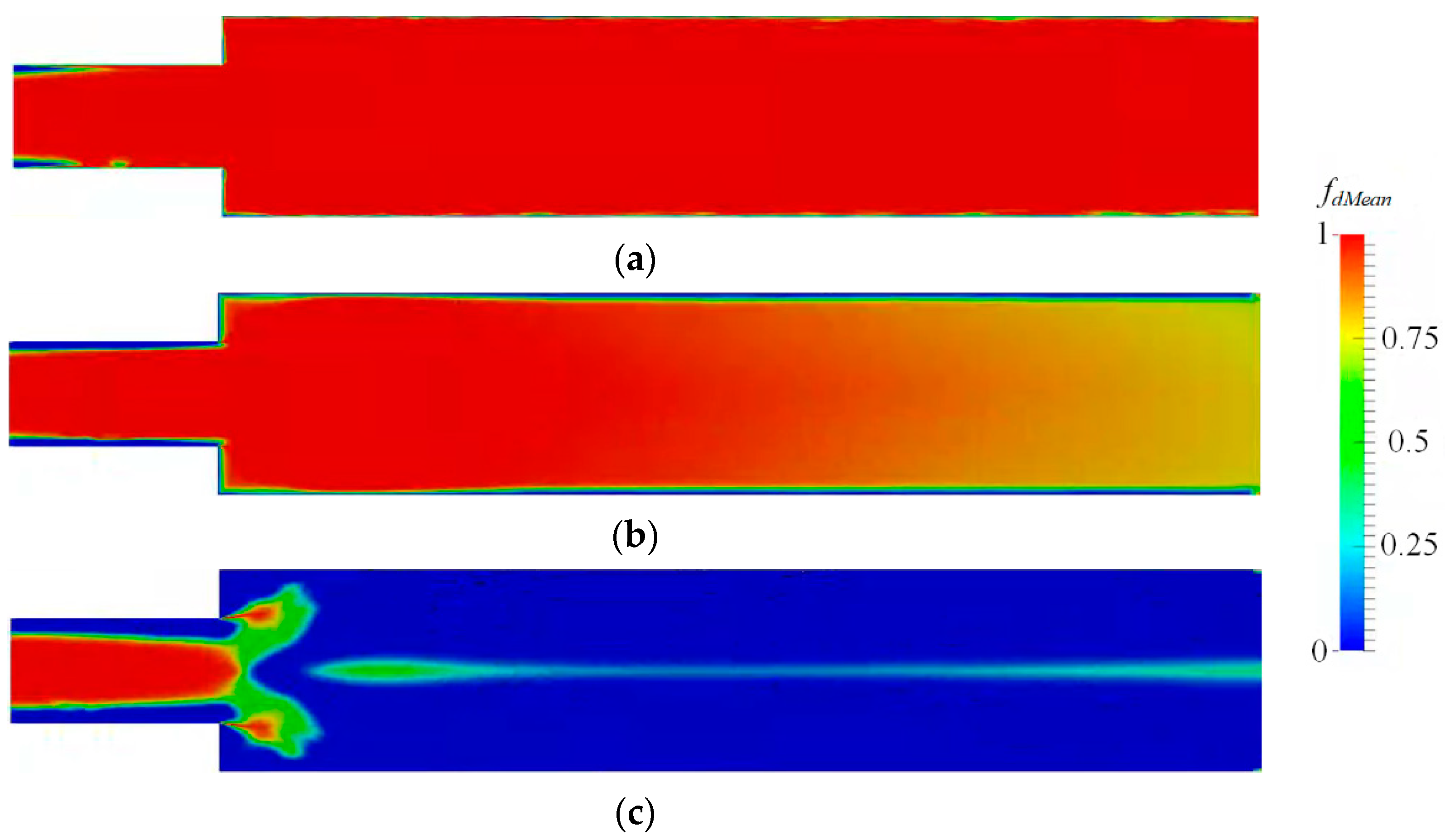
Figure 5 shows the contour of the f d variable with three DDES-type models. f d = 0 represents the URANS branch used, and f d = 1 represents the eddy simulation branch used. It can be seen that the DDESO model stays in the URANS model for the whole channel. The BADDES and ADDES models stay in the URANS model only in the near-wall region, and eddy simulation branches are used in most areas. Compared with the ADDES model, the URANS region of the BADDES model is thinner, which means that the model can switch from the URANS branch to the eddy simulation branch faster.
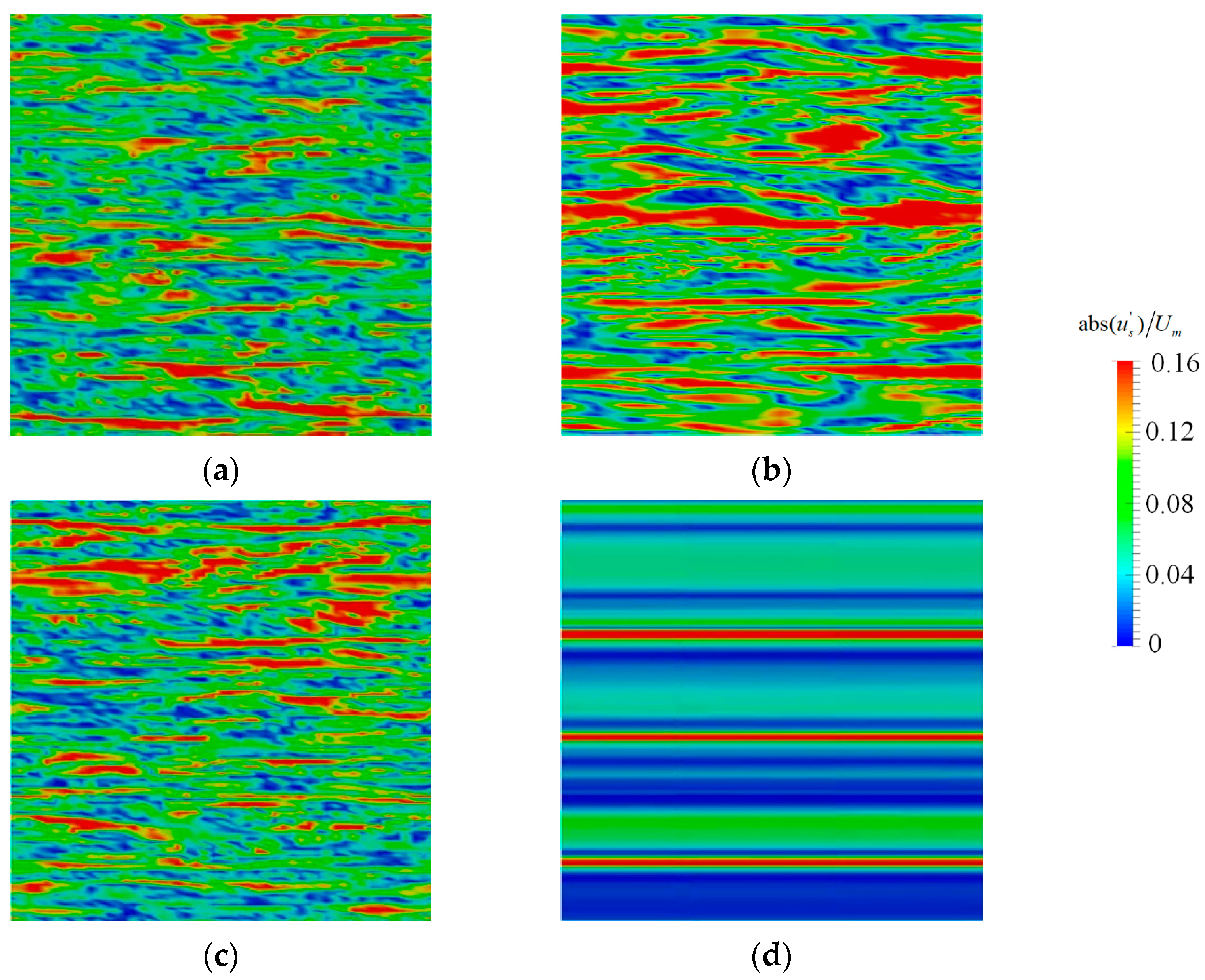
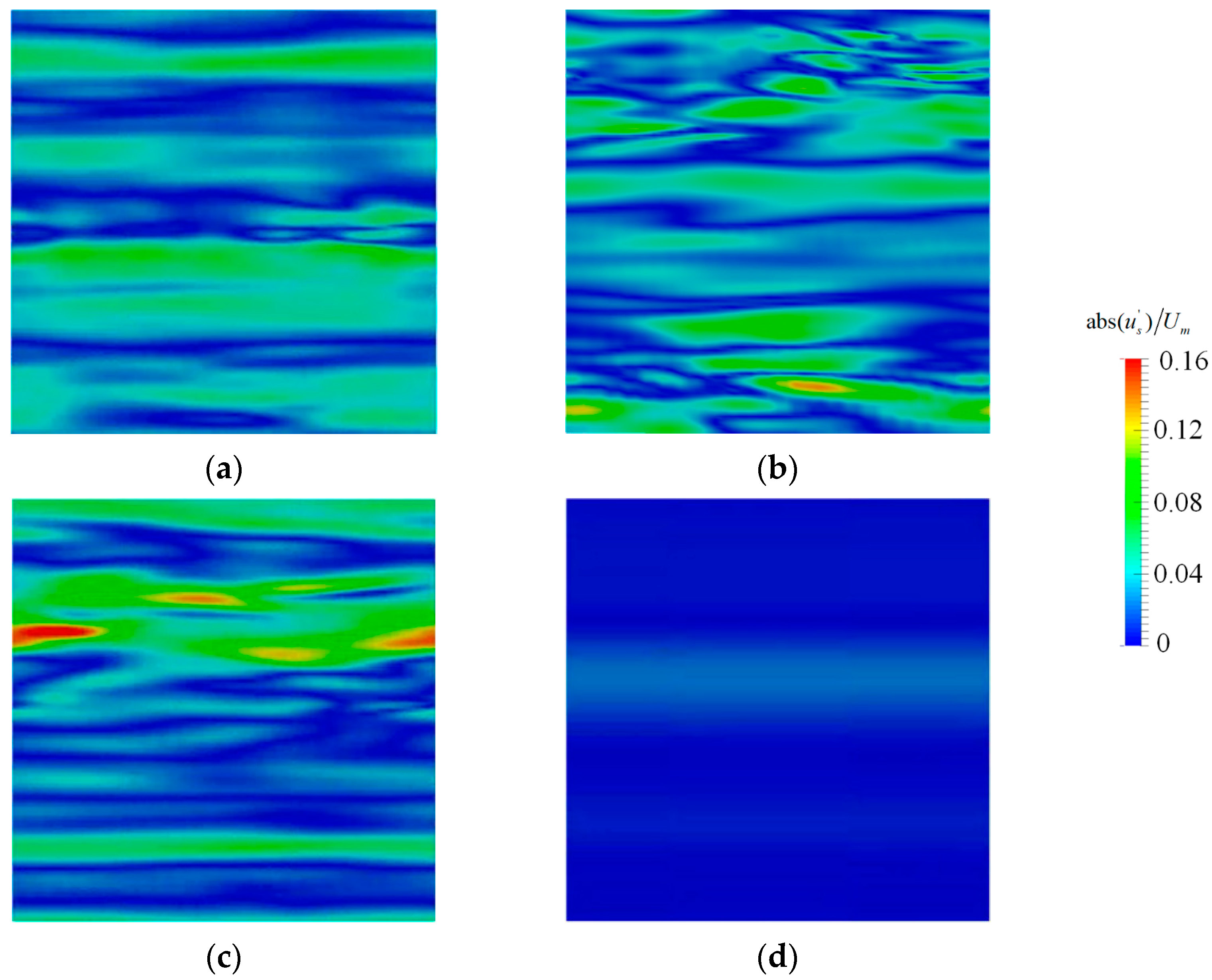
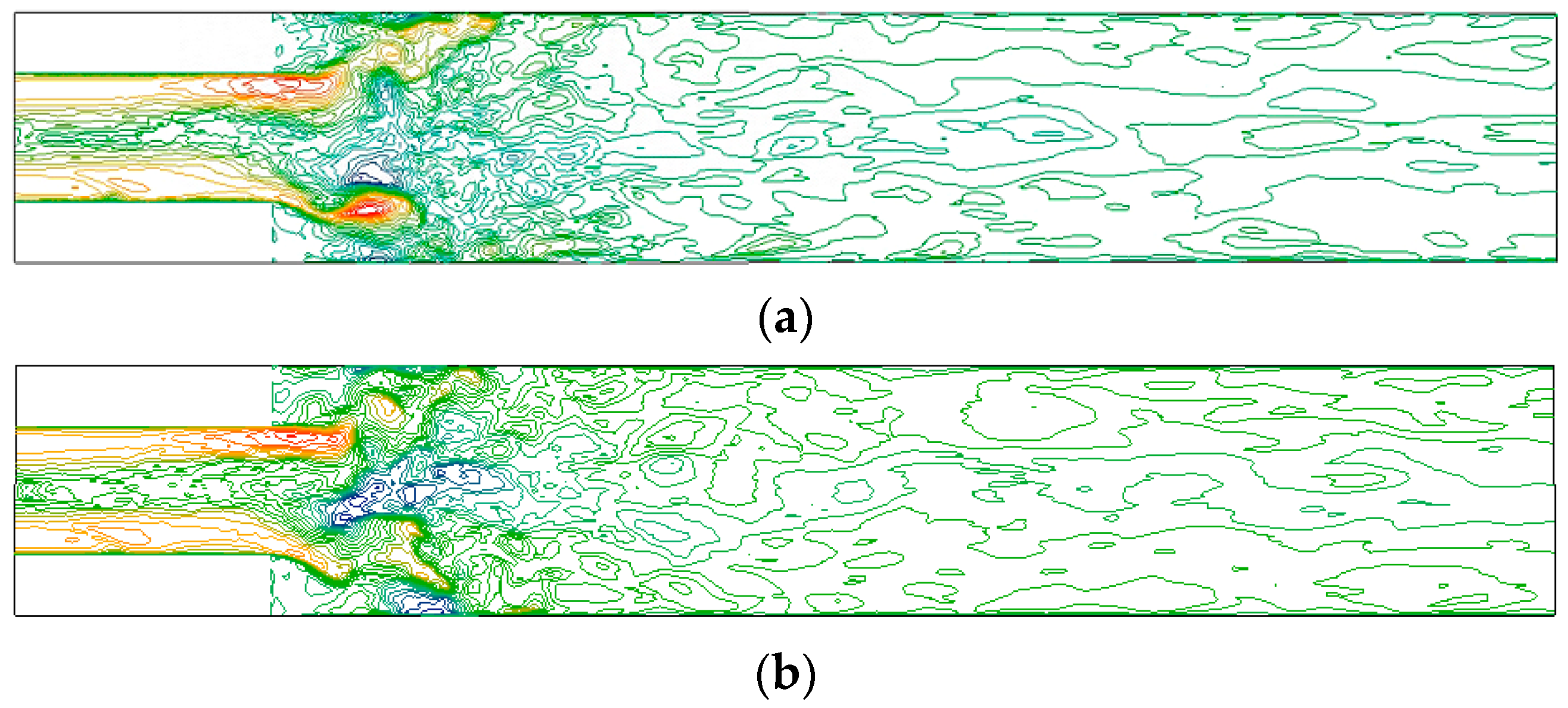
Figure 6 and Figure 7 show the transient fluctuation velocity distributions in the near-wall region with different turbulence models at y/h = 0.4 and y/h = 1.96, respectively. The plane y/h = 0.04 is the position with the streamwise fluctuation velocity peak values by the BADDES model on the pressure side, while the plane y/h = 1.96 is at the same position of the suction side for comparison with the results on the pressure side.
Figure 6 shows streak structures with a staggered distribution of high-velocity and low-velocity areas at y/h = 0.04. The fluctuation velocity distribution near the pressure side of the BADDES model and BkO model are similar and show that the streak structures are smaller in scale and greater in number, which is consistent with the results of Yang et al. [51]. The streak structures of the ADDES model are relatively large in scale and fewer in number than the BADDES model. In addition, the DDESO model only shows the very large-scale streak characteristic.
Figure 7 shows that the streak structure becomes enormous in scale and smaller in number at y/h = 1.96. This indicates that the turbulence is suppressed on the suction side due to the rotation effects. In addition, the streak structure of the BADDES, ADDES, and BkO models are far superior to those of the DDESO model, indicating that the DDESO model cannot resolve the fluctuation velocity.
The Q-criterion was applied to demonstrate the vortex structure in the rotating channel flow:
Q = 1 2 ( Ω i j Ω i j S i j S i j ) .
where Ω i j and S i j are the rotation rate and strain rate tensors, respectively. Figure 8a–c shows the vortex structure with Q = 0.0025 s−2 at a particular time calculated using the BADDES, ADDES, and BkO models, respectively. Figure 8d shows the vortex structure with Q = 0.0003 s−2 calculated by the DDESO model. It uses a larger threshold to show the deviation among the three turbulence models clearly. The isosurface of Q is colored using the magnitude of the mean flow velocity.
Figure 8 clearly shows that the DDESO model only captures fewer vortex structures. Compared with the ADDES model, the BADDES model can capture smaller-scale vortex structures. In addition, there are more vortex structures on the pressure side and fewer on the suction side, owing to the rotation effect.

3.1.3. Comparison of Computational Cost

The computational cost should be analyzed to ensure the engineering practicality of the BADDES model. The average time for iteration is calculated on the same workstation to study the computational cost of the different models. The CPU is a Xeon platinum 8259L, with 48 cores, 96 threads, and 2.50 GHz, and parallel simulation is conducted with 48 cores. The same boundary conditions and initial conditions were adopted for all the calculations. One thousand time steps are calculated for each model, repeated three times, and the average value is taken to obtain the iteration time of each step. Table 1 shows the results.
Table 1 shows the average time for iteration with the four different turbulence models. The calculation cost of the BADDES model is the smallest. Compared with the BADDES model, the calculation cost of the ADDES model, the BkO model, and the DDESO model is 3.07%, 11.66%, and 11.25% higher, respectively.

3.2. Taylor-Couette Flow

3.2.1. Benchmark Description and Computational Setup

The second case is Taylor-Couette flow, a flow type with wall rotation and curvature effect. The physical model of Taylor-Couette flow is two concentric cylinders. When one of the cylinders rotates, it will cause fluid movement. Since Taylor-Couette flow contains rotation and curvature effects, this case is widely used as a simplified model of rotating machinery in studies.
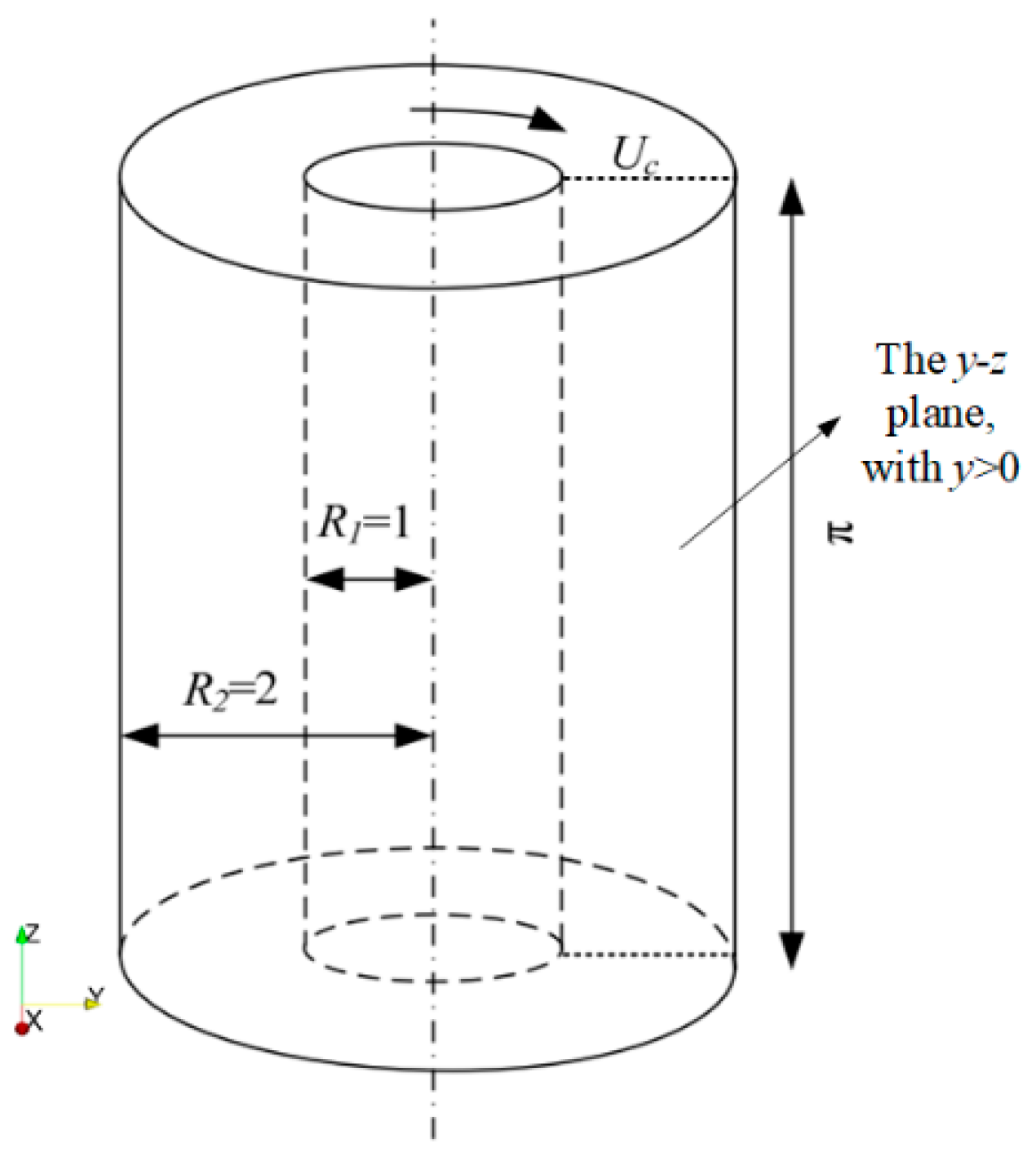
In this section, the DNS data from the Reference of Dong [54] are compared with the BADDES model, ADDES model, BkO model, and DDESO model. Figure 9 is a sketch of the Taylor-Couette flow. The outer cylinder is fixed while the inner cylinder rotates at a constant angular velocity. The radius of the inner cylinder is R 1 = 1 , where U 0 is the rotation velocity of the inner cylinder. The radius of the outer cylinder is R 2 = 2 . The length of the axis is π and the gap width is d = R 2 R 1 . The Reynolds number is defined as Re = U 0 d / υ , where ν is the kinematic viscosity of the fluid. We have simulated the Reynolds numbers as 8000.
The number of nodes used in the circumferential, radial, and axial directions is 128, 32, and 64, respectively. The circumferential and axial grids are uniformly distributed, and the radial is locally encrypted in the near-wall area. The axial direction is set as periodic boundary conditions; the inner cylindrical surface is a rotating wall, and the azimuthal velocity is set to U 0 ; the outer cylindrical surface is a non-slip wall. There is no system rotation in this case, so the governing equations are the same as Equations (31) and (32), but without the Coriolis body force. The incompressible solver pisoFoam is used to solve the governing equation. The time is constant in the calculation process, and the maximum CFL number does not exceed 1. The calculation reaches a stable state after about 20 rotation cycles of 2 π R 2 / U 0 . At this time, the circumferential velocity shows regular periodic changes. Therefore, the whole simulation calculated a total of about 400 rotation cycles. The first twenty rotation cycles were used to eliminate the transient characteristics of the flow, and the last 380 rotation cycles were averaged.

3.2.2. Results and Discussion

Similar to the results of the rotating channel flow, the quantitative results of this case have been averaged over time, circumferential direction, and axial direction.
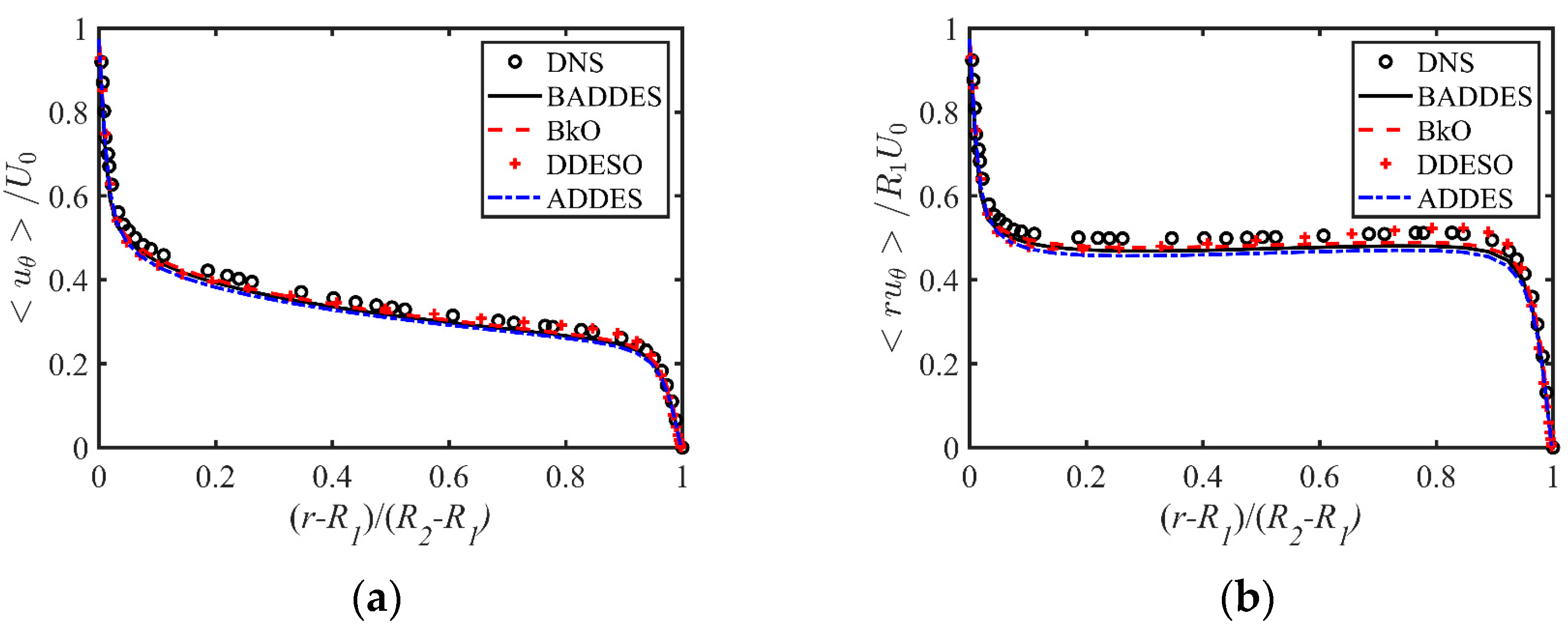
Figure 10 shows the distribution of mean azimuthal velocity and the mean angular momentum at the two Reynolds numbers with different models. The mean velocity has been normalized by U 0 and the mean angular momentum by R 1 U 0 .
Figure 10a shows that the overall azimuthal velocity gradually decreases along the radial direction from the inner wall surface. Note the asymmetry of the mean velocity profiles at the inner and outer cylinder walls. In the inner cylindrical surface, the azimuthal velocity is the wall rotation velocity U 0 , and the outer cylindrical surface velocity is 0. In the area near the wall, the azimuthal velocity decays rapidly due to the shearing effect, while in the core area of the flow 0.1 ( r R 1 ) / ( R 2 R 1 ) 0.9 , the azimuthal velocity decreases linearly and slowly with the radial velocity. Figure 10b shows the essentially constant mean angular momentum in the core area of the flow [55,56,57]. Figure 10 also shows that the prediction results of the four models are very close. The relative error was used to quantitatively express the deviation between different models and DNS results. The quantitative deviation of the BADDES model, ADDES model, BkO model, and DDESO model is 4.87%, 7.11%, 4.03%, and 6.4%, respectively.
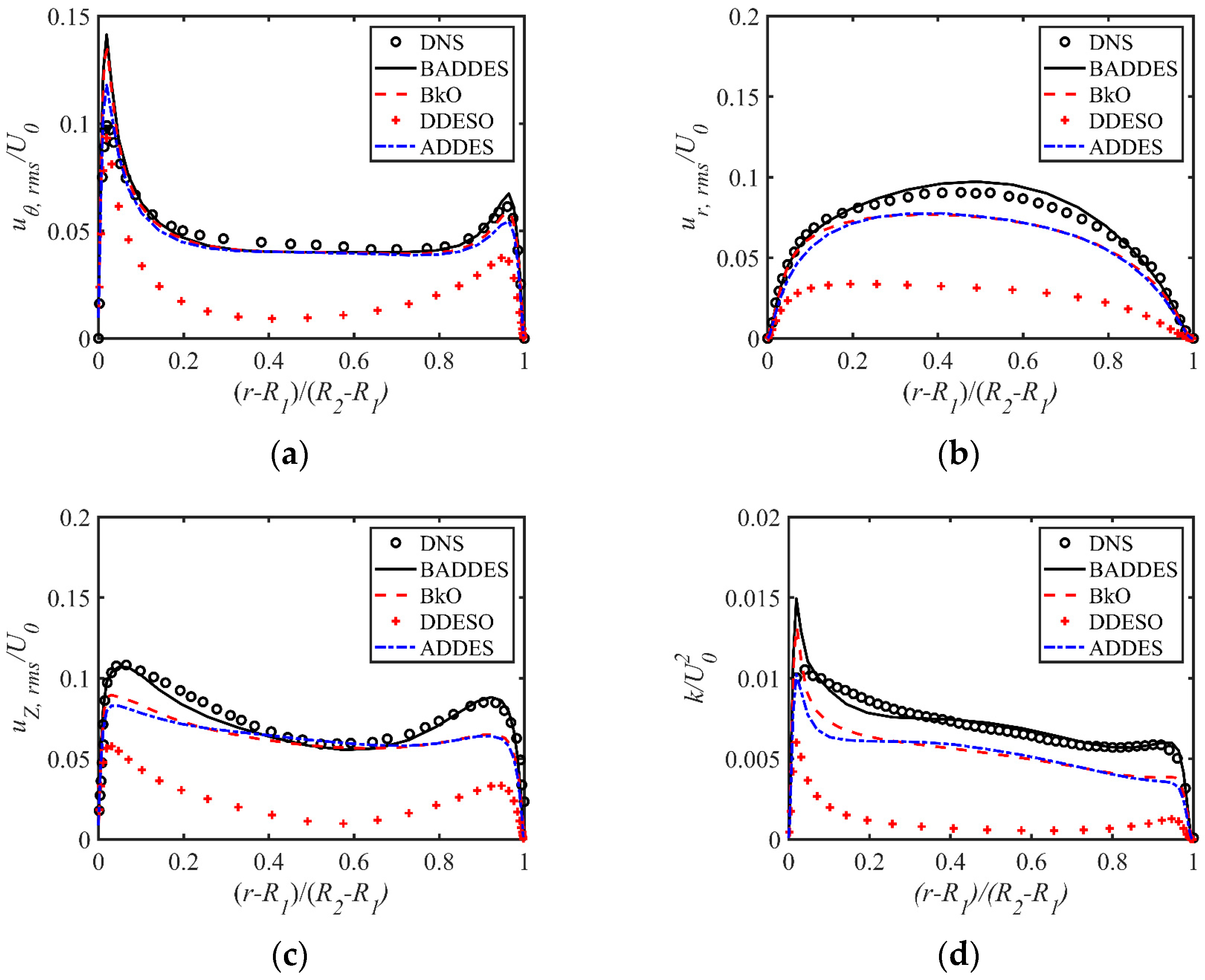
Figure 11 compares the RMS fluctuation velocity (normalized by U 0 ) and turbulent kinetic energy (normalized by U 0 2 ) profiles of different turbulence models. In addition to the RMS of the azimuthal fluctuation velocity, other DNS results of the RMS of the fluctuation velocity were extracted from the study by Chouippe et al. [58]. Since there is no result for the Reynolds shear stress in the study, no comparison is made in the present work.
As for the azimuthal fluctuation velocity, Figure 11a shows that the peak values of the inner wall are substantially higher than those of the outer wall, indicating that the most energetic turbulence occurs near the inner cylinder wall. It also shows that the prediction results of the BADDES and BkO models are very close and slightly worse than the ADDES model, while the deviation between the DDESO model and DNS results is relatively large. As for the radial fluctuation velocity, the axial fluctuation velocity, and the turbulent kinetic energy, Figure 11b–d shows that the result of the BADDES model is superior to those of the ADDES model and BkO model, especially in the near-wall region. In addition, the three models are far superior to the DDESO model.
The relative error was used to quantitatively express the deviation between the different turbulence models and DNS results. Table 2 shows the relative errors of the RMS velocity calculated by different turbulence models.
Similar to the results of Figure 11, the BADDES model is slightly superior to the ADDES model and BkO model. All three models are far superior to the DDESO model. At the same time, Table 2 also shows that the deviation of the BADDES model is less than that of the ADDES model by about 5.32%. The quantitative average deviation of the BADDES model, ADDES model, BkO model, and DDESO model is 11.96%, 17.28%, 15.61%, and 56.82%, respectively.
Figure 12 shows the contour of the f d variable with three DDES-type models in the y-z plane (y > 0). The position is marked in Figure 9. Similar to Figure 5, the DDESO model stays in the URANS model for most of the computation region. The BADDES and ADDES models stay in the URANS model only in the near-wall region, and the URANS region of the BADDES model is thinner than that of the ADDES model.
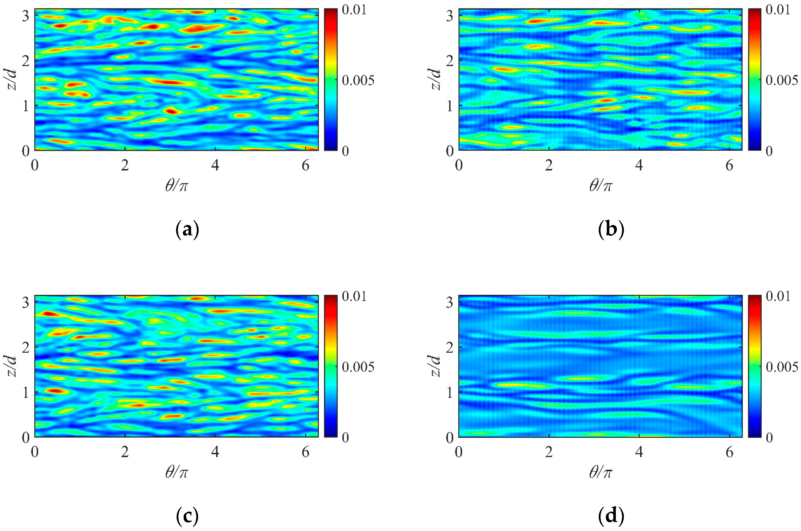
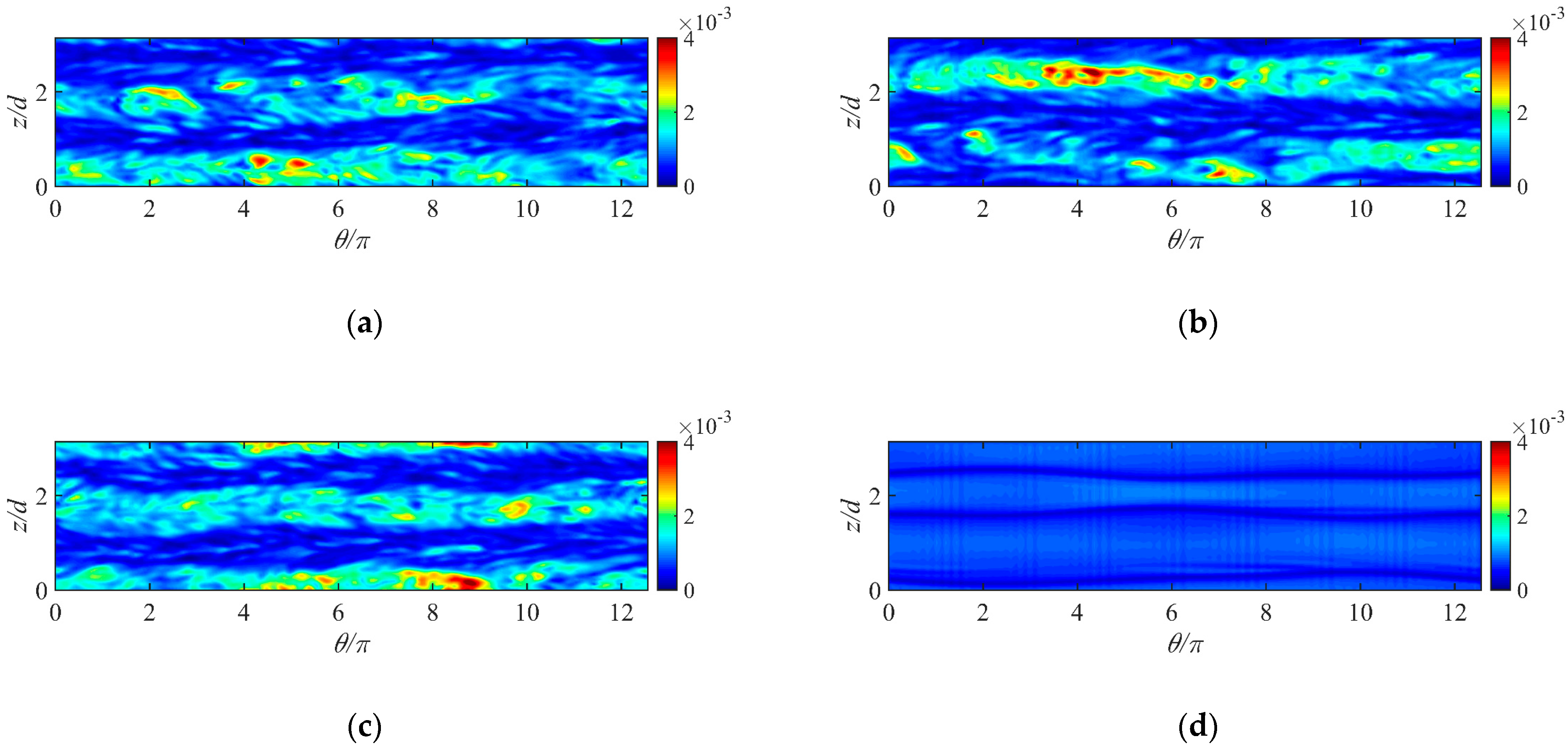
Figure 13 and Figure 14 show the expansion diagram of the instantaneous wall shear stress distribution on the inner and outer cylindrical surfaces, respectively. The wall shear stress is τ w = v ( u / y ) y = 0 normalized by τ w / U 0 2 , the abscess is the angle normalized by π , and the ordinate is the axial distance normalized by d. The shear stress value is represented by color, and the “Jet” type color bar is used in MATLAB.
In the inner cylinder, the wall shear stresses show a herringbone structure with alternating high and low levels. The herringbone structures predicted by the DDESO model are simple in their distribution and few in number. The BADDES model, ADDES model, and BkO model can predict many small and disordered herringbone structures, reflecting turbulence’s random and disordered characteristics.
There is a large velocity gradient in the inner cylinder due to the fluid motion caused by the rotation of the inner cylinder. Therefore, Figure 13 and Figure 14 show that the wall shear stress of the inner cylinder is much larger than that of the outer cylinder. In addition, there are no apparent herringbone structures on the outer cylinder wall.
Figure 13 and Figure 14 also show that the prediction results of the BADDES model are similar to those of the BkO model. Because the same bifurcation k ω model was used in the near-wall region, richer flow field information can be obtained than with the ADDES model or the DDESO model.

3.2.3. Comparison of Computational Cost

The same workstation was used to study the computational cost of the four turbulence models in the Taylor-Couette flow. The same boundary conditions and initial conditions were adopted for all four turbulence models. One thousand time steps are calculated for each model, repeated three times, and the average value is taken to obtain the iteration time of each step. Table 3 shows the results.
Table 3 shows the average time for iteration with the four different turbulence models in the Taylor-Couette flow. It can be seen that the calculated cost of the BADDES model is also the smallest. In addition, the calculation cost of the ADDES and the DDESO models is about twice that of the BADDES model, which is quite different from that of the rotating channel flow. There is little difference in the calculation cost of the BkO model between the rotating channel flow and the Taylor-Couette flow, and the calculation cost increases by 8.35% compared with the BADDES model.

3.3. Swirling Flow through an Abrupt Axisymmetric Expansion

3.3.1. Benchmark Description and Computational Setup

The third case is swirling flow through an abrupt axisymmetric expansion, a flow type with the inlet swirling flow and sudden expansion. Therefore, the flow has a large adverse pressure gradient and complex turbulence characteristics, involving the formation, shedding, reattachment, and collapse of the rotating separation vortex. The calculation domain of the abrupt axisymmetric expansion in the present work is consistent with H. Nilsson’s [59] work. There are two parts of the calculation domain: the incoming flow pipe section and the downstream pipe section, where the expansion ratio is D o u t / D i n = 1.94 . The physical model is shown in Figure 15. This paper calculates the working conditions of the Reynolds number as 30,000, and the swirl number is 0.6. The experimental data are from Foroutan and Yavuzkurt [60].
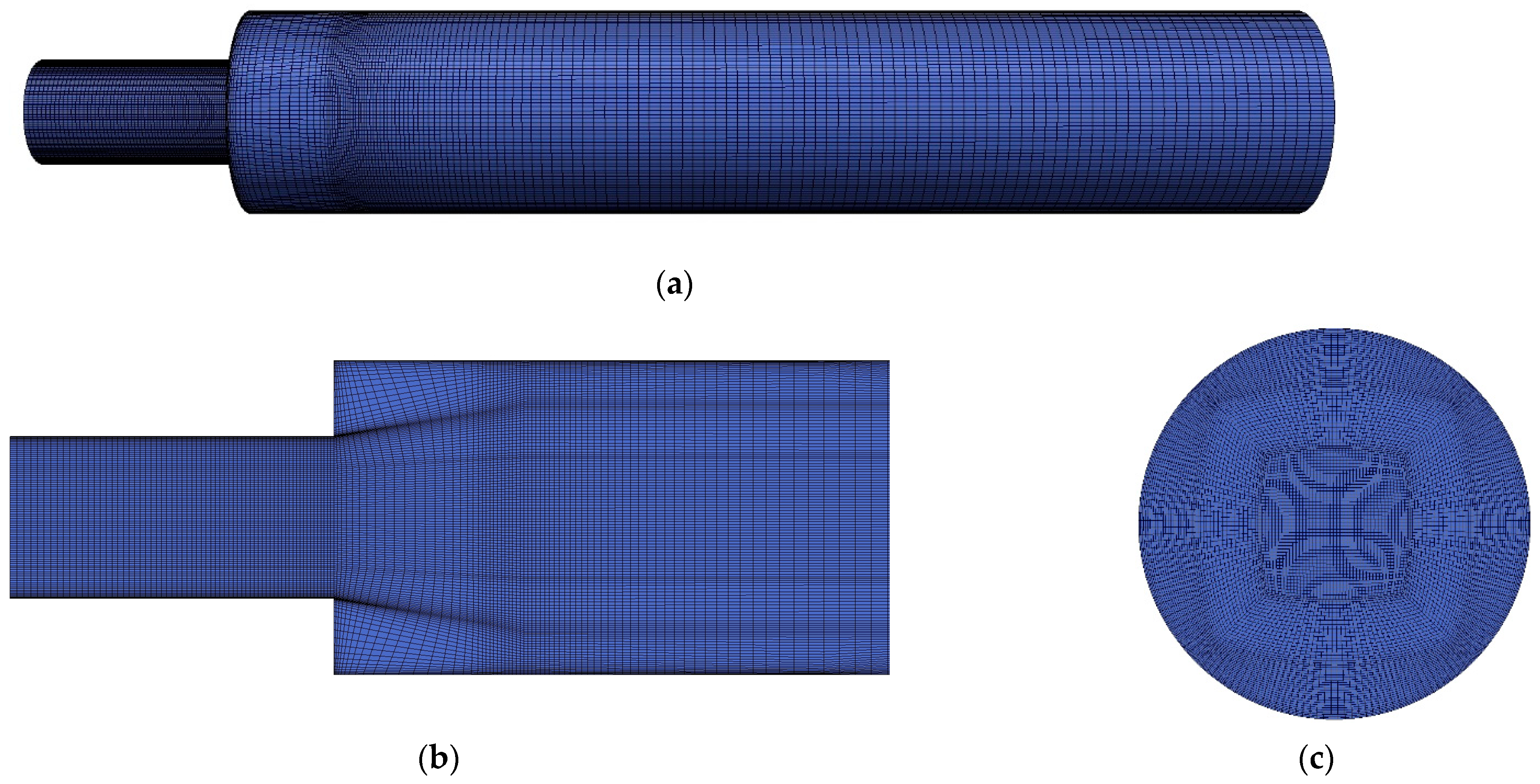
The total number of grids is 1.66 million, and y+ < 5. This grid number is verified by Foroutan and Yavuzkurt [60] to be suitable for solving the hybrid turbulence models. Figure 16 shows the schematic diagram of the mesh used in the swirling flow through an abrupt expansion.
In this paper, the experimentally measured average velocity value is used as the velocity inlet condition, the non-slip boundary condition is used on the wall, and the zeroGradient boundary condition is used at the outlet. In this case, the governing equations are the same as the Taylor-Couette flow. The incompressible flow solver pimpleFoam is used to solve the governing equation. In the calculation process, the time step can be automatically adjusted to meet CFL < 1.5, which is conducive to better convergence.
The calculation reaches a stable state after about 0.25 flow cycles. Therefore, the whole simulation calculated a total of about five flow cycles. The first 0.25 flow cycles were used to eliminate the transient characteristics of the flow, and the last 4.75 cycles were averaged.

3.3.2. Results and Discussion

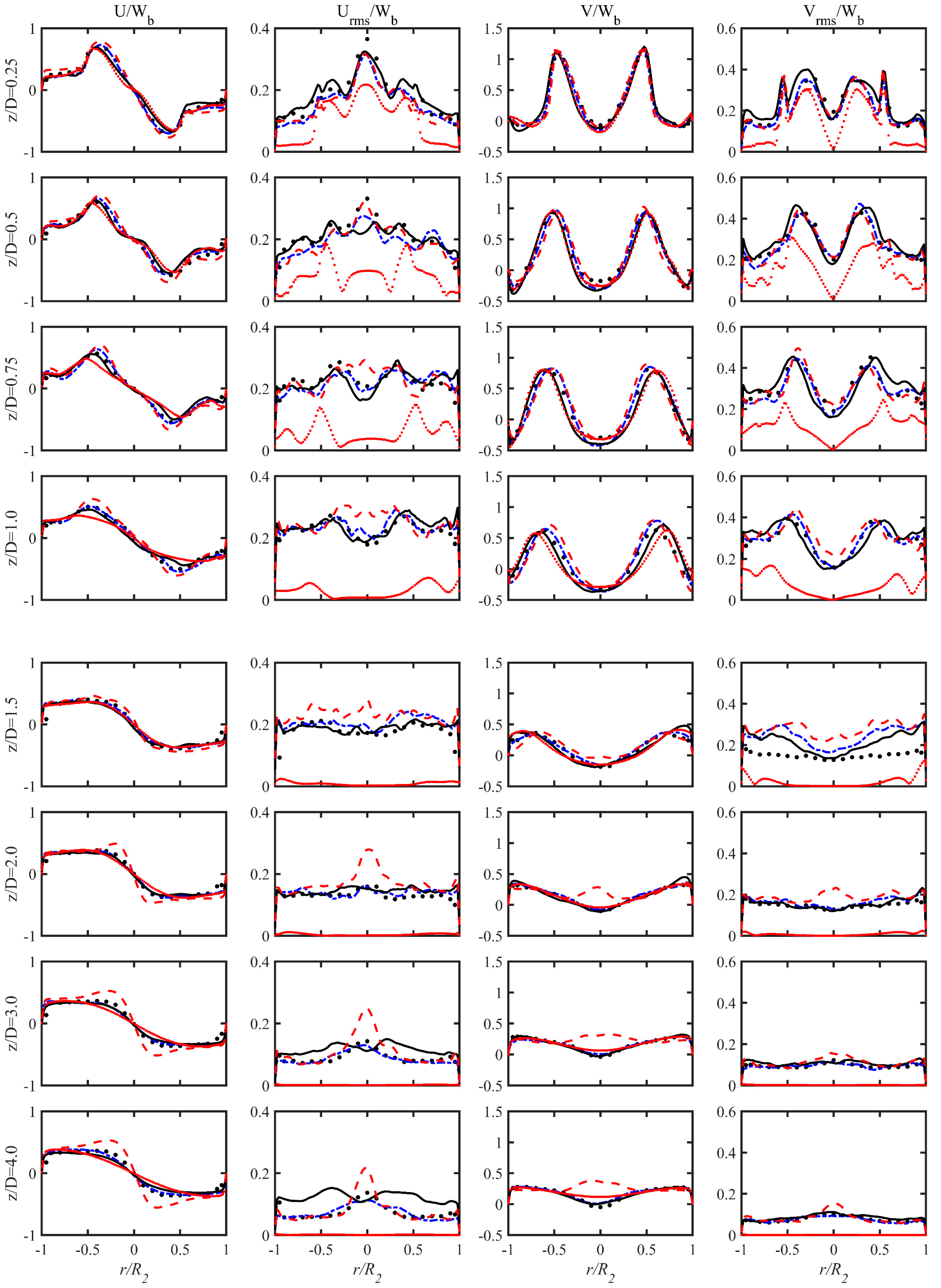
Figure 17 shows the radial distributions of the mean circumferential and axial velocity and mean circumferential and axial RMS velocity downstream of the expansion at different positions.
The overall distribution is in a reverse “S” shape for the mean circumferential velocity, and the characteristics of the reverse “S” shape distribution form are weakened as the downstream distance increases. Near where the flow suddenly separates, two peaks with opposite velocity directions decrease as the downstream distance increases. For the mean axial velocity, there are two symmetrically distributed peaks, which are “M”-shaped distributions, the peak points decrease as the downstream distance increases, and the velocity distribution presents a “V”-shaped distribution at Z/D = 2. The results of the BADDES and ADDES models are similar and superior to the BkO model and the DDESO model. In addition, the BkO model predicted an abnormally positive value in the middle of the pipeline after Z/D ≥ 2. It may be related to the defect of the k ω model; that is, the ω-equation has a strong sensitivity to the values of ω in the freestream outside the boundary layer.
As for the mean circumferential and axial RMS velocity, Figure 17 shows that the BADDES model is superior to the ADDES model. Meanwhile, both the BADDES and ADDES models are superior to the BkO model and the DDESO model. The former overestimates the RMS velocity at the center of the pipeline, and the latter tends to converge upon a steady solution leading to a relatively small RMS velocity.
Figure 18 shows the contour of the f d variable with three DDES-type models. Figure 18 shows that the DDESO model only stays in the eddy simulation branch for the incoming flow pipe section and then switches to the URANS model faster in the downstream pipe section. The BADDES and ADDES models stay in the URANS model only in the near-wall region, and eddy simulation branches are used in most areas. The URANS region of the BADDES model is smaller than that of the ADDES model.
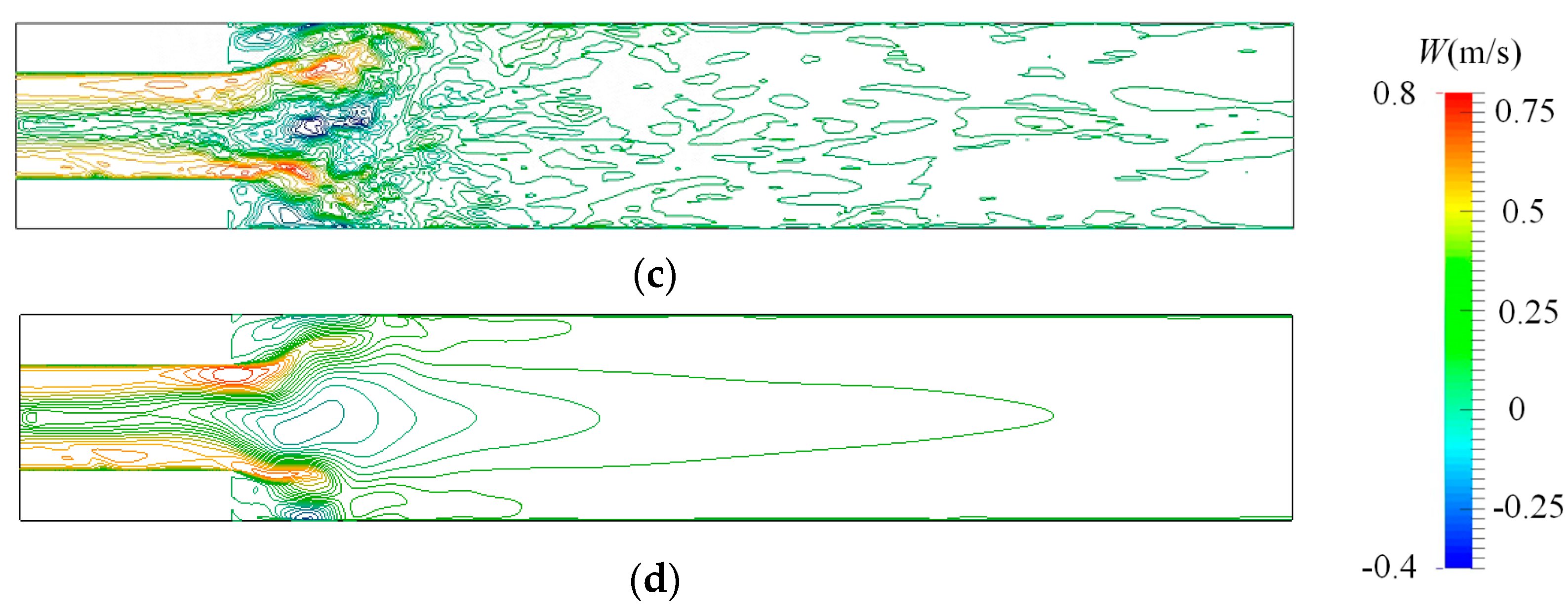
Figure 19 shows the transient axial velocity contour plots of different turbulence models. The contour levels are between −0.4 and 0.8 at intervals of 0.05. It can be seen that the BADDES model, the ADDES model, and the BkO model can capture abundant turbulence characteristics at the center of the pipe near the abrupt expansion region. In addition, the results of the BADDES model are slightly more abundant than those of the ADDES and BkO models. Meanwhile, the DDESO model fails to capture these turbulence characteristics, which appear to be steady symmetric results, although the URANS equations were solved.
Figure 20 shows the iso-surfaces of the Q-criterion with a value of 1200 s−2 to visualize the three-dimensional vortical structures. The iso-surface of Q is colored using the magnitude of the transient axial velocity.
A three-dimensional vortex structure similar to a cylinder appears in the center of the upstream pipe, rapidly changing into an irregular small-scale vortex structure at the sudden expansion. It can clearly be seen that the BADDES model, ADDES model, and BkO model capture a greater number of small-scale vortex structures. However, the BkO model over-predicted the vortex structures in the middle position downstream of the pipeline. The number of captured vortex structures of the DDESO model is the lowest.

3.3.3. Comparison of Computational Cost

The same workstation was used to study the computational cost of the four turbulence models in the flow through an abrupt axisymmetric expansion. The same boundary conditions and initial conditions were adopted for all four turbulence models. In the present work, the pimpleFoam solver was set to iterate six times within a time step. Therefore, 2000 time steps were calculated for each model, and 12,000 iteration steps were calculated. Each calculation was repeated three times, and the time of each iteration step was averaged.
Table 4 shows the average iteration time of the four different turbulence models in the swirling flow through an abrupt axisymmetric expansion. The calculated cost of the BADDES model is slightly less than that of the ADDES model. In addition, the calculation cost of the BADDES model is 12.593% lower than that of the BkO model.

4. Conclusions

Based on the bifurcation approach, the k ω model is modified to account for the effects of rotation and curvature and then used as a base model to establish a new adaptive DDES method. The BADDES model was simulated in rotating channel flow with system rotation, Taylor-Couette flow with wall rotation and curvature effect, and swirling flow through an abrupt axisymmetric expansion with inlet swirling flow to study its prediction effect. Three k ω -type models (ADDES, BkO, and DDESO) were also simulated for comparison.
  • Regarding the velocity of the rotating channel flow with system rotation, the BADDES, ADDES, and BkO models can capture the rotation effect, while the DDESO model cannot capture the rotation effect. As for the other two cases, the velocity distribution is close, and the BADDES and ADDES models are slightly superior to the BkO and DDESO models.
  • Regarding the RMS velocity, the results of the BADDES model are slightly superior to those of the ADDES model and the BkO model. Meanwhile, the BADDES, ADDES, and BkO models are far superior to the DDESO model, especially in the swirling flow through an abrupt axisymmetric expansion, which tends to converge upon a steady solution leading to a relatively small RMS velocity.
  • The ADDES model sustained a certain RANS region thickness, even on grids with a resolution suitable for wall-resolved LES. Compared with the ADDES model, the URANS region of the BADDES model is thinner with the same grids. Thus, a DDES model based on the bifurcation URANS model can alleviate the SLD problem. Meanwhile, the DDESO model stays in the URANS model for most computed regions in all three cases.
  • The BADDES model and the BkO model capture a more abundant number of small-scale vortex structures than the ADDES model. However, the BkO model over-predicted the vortex structures in the middle position downstream of the pipeline. In addition, the DDESO model captures significantly fewer vortex structures.
  • The computation cost (average iteration time) of the BADDES model is slightly less than that of the ADDES model in the rotating channel flow and the swirling flow through an abrupt axisymmetric expansion: 3.07% and 1.72% lower, respectively. In addition, the calculation cost of the ADDES model is about twice that of the BADDES model in the Taylor-Couette flow.

Author Contributions

Conceptualization, Z.L. and K.P.; methodology, K.P. and X.H.; software, K.P. and X.H.; validation, K.P., Y.L. and W.Y.; formal analysis, K.P.; investigation, W.Y.; resources, K.P.; data curation, Z.L.; writing—original draft preparation, K.P.; writing—review and editing, X.H. and Z.L.; visualization, Y.L.; supervision, X.H.; project administration, Y.L.; funding acquisition, Z.L. and X.H. All authors have read and agreed to the published version of the manuscript.

Funding

This research was funded by the National Natural Science Foundation of China, grant numbers 52179093 and 51909231, and the Open Research Subject of Key Laboratory of Fluid and Power Machinery (Xihua University), Ministry of Education, grant number LTDL2021-009. This research was also funded by the Jiangsu Funding Program for Excellent Postdoctoral Talent.

Institutional Review Board Statement

Not applicable.

Informed Consent Statement

Not applicable.

Data Availability Statement

The data that support the findings of this study are available from the corresponding author upon reasonable request.

Acknowledgments

The authors are grateful to Paul Durbin and Zifei Yin for their help with model implementation. The authors also acknowledge the reviewers and the editors for their comments to improve the quality of this paper.

Conflicts of Interest

The authors declare no conflict of interest.

References

  1. Lavis, D.R.; Forstell, B.G.; Purnell, J.G. Compact waterjets for high-speed ships. Ships Offshore Struct. 2007, 2, 115–125. [Google Scholar] [CrossRef]
  2. Hu, F.F.; Wu, P.; Wu, D.Z.; Wang, L.Q. Numerical study on the stall behavior of a water jet mixed-flow pump. J. Mar. Sci. Technol. 2014, 19, 438–449. [Google Scholar] [CrossRef]
  3. Li, C.; Weijun, Q. Rotating stall region of water-jet pump. Trans. Famena 2014, 38, 31–40. [Google Scholar]
  4. Zhang, Y.; Wu, Y. A review of rotating stall in reversible pump turbine. Proc. Inst. Mech. Eng. Part C J. Mech. Eng. Sci. 2017, 231, 1181–1204. [Google Scholar] [CrossRef] [Green Version]
  5. Xia, C.; Cheng, L.; Luo, C.; Jiao, W.; Zhang, D. Hydraulic characteristics and measurement of rotating stall suppression in a waterjet propulsion system. Trans. Famena 2018, 42, 85–100. [Google Scholar] [CrossRef]
  6. Zhang, L.; Zhang, J.N.; Shang, Y.C. A potential flow theory and boundary layer theory based hybrid method for waterjet propulsion. J. Mar. Sci. Eng. 2019, 7, 113. [Google Scholar] [CrossRef] [Green Version]
  7. Durbin, P.A. Some Recent Developments in Turbulence Closure Modeling. Annu. Rev. Fluid Mech. 2018, 50, 77–103. [Google Scholar] [CrossRef]
  8. Huang, X.; Yang, W.; Li, Y.; Qiu, B.; Guo, Q.; Liu, Z. Review on the sensitization of turbulence models to rotation/curvature and the application to rotating machinery. Appl. Math. Comput. 2019, 341, 46–69. [Google Scholar] [CrossRef]
  9. Yin, Z.; Reddy, K.R.; Durbin, P.A. On the dynamic computation of the model constant in delayed detached eddy simulation. Phys. Fluids 2015, 27, 025105. [Google Scholar] [CrossRef] [Green Version]
  10. Spalart, P.R.; Shur, M. On the Sensitization of Turbulence Models to Rotation and Curvature. Aerosp. Sci. Technol. 1997, 1, 297–302. [Google Scholar] [CrossRef]
  11. Fröhlich, J.; Von Terzi, D. Hybrid LES/RANS methods for the simulation of turbulent flows. Prog. Aerosp. Sci. 2008, 44, 349–377. [Google Scholar] [CrossRef]
  12. Spalart, P.R.; Deck, S.; Shur, M.L.; Squires, K.D.; Strelets, M.K.; Travin, A. A new version of detached-eddy simulation, resistant to ambiguous grid densities. Theor. Comput. Fluid Dyn. 2006, 20, 181–195. [Google Scholar] [CrossRef]
  13. Menter, F.R.; Kuntz, M.; Langtry, R. Ten Years of Industrial Experience with the SST Turbulence Model. Turbul. Heat Mass Transf. 2003, 4, 625–632. [Google Scholar]
  14. Shur, M.L.; Spalart, P.R.; Strelets, M.K.; Travin, A.K. A hybrid RANS-LES approach with delayed-DES and wall-modelled LES capabilities. Int. J. Heat Fluid Flow 2008, 29, 1638–1649. [Google Scholar] [CrossRef]
  15. Spalart, P.R. Detached-eddy simulation. Annu. Rev. Fluid Mech. 2009, 41, 181–202. [Google Scholar] [CrossRef]
  16. Menter, F. Stress-Blended Eddy Simulation (SBES)—A New Paradigm in Hybrid RANS-LES Modeling. Prog. Hybrid RANS-LES Model. 2018, 137, 27–37. [Google Scholar] [CrossRef]
  17. Reddy, K.R.; Ryon, J.A.; Durbin, P.A. A DDES model with a Smagorinsky-type eddy viscosity formulation and log-layer mismatch correction. Int. J. Heat Fluid Flow 2014, 50, 103–113. [Google Scholar] [CrossRef]
  18. He, X.; Zhao, F.; Vahdati, M. Detached Eddy Simulation: Recent Development and Application to Compressor Tip Leakage Flow. J. Turbomach. 2022, 144, 1–10. [Google Scholar] [CrossRef]
  19. Chauvet, N.; Deck, S.; Jacquin, L. Zonal Detached Eddy Simulation of a Controlled Propulsive Jet. AIAA J. 2007, 45, 2458–2473. [Google Scholar] [CrossRef]
  20. Mockett, C.; Fuchs, M.; Garbaruk, A.; Shur, M.; Spalart, P.; Strelets, M.; Thiele, F.; Travin, A. Two non-zonal approaches to accelerate RANS to LES transition of free shear layers in DES. Notes Numer. Fluid Mech. Multidiscip. Des. 2015, 130, 187–201. [Google Scholar] [CrossRef]
  21. Shur, M.L.; Spalart, P.R.; Strelets, M.K.; Travin, A.K. An Enhanced Version of des with Rapid Transition from RANS to LES in Separated Flows. Flow Turbul. Combust. 2015, 95, 709–737. [Google Scholar] [CrossRef]
  22. Yin, Z.; Durbin, P.A. An adaptive DES model that allows wall-resolved eddy simulation. Int. J. Heat Fluid Flow 2016, 62, 499–509. [Google Scholar] [CrossRef]
  23. He, C.; Liu, Y.; Yavuzkurt, S. A dynamic delayed detached-eddy simulation model for turbulent flows. Comput. Fluids 2017, 146, 174–189. [Google Scholar] [CrossRef]
  24. He, C.; Liu, Y. A dynamic detached-eddy simulation model for turbulent heat transfer: Impinging jet. Int. J. Heat Mass Transf. 2018, 127, 326–338. [Google Scholar] [CrossRef]
  25. Yin, Z.; Ge, X.; Durbin, P. Adaptive detached eddy simulation of transition under the influence of free-stream turbulence and pressure gradient. J. Fluid Mech. 2021, 915, 1–26. [Google Scholar] [CrossRef]
  26. Li, F.; He, C.; Wang, P.; Liu, Y. Unsteady analysis of turbulent flow and heat transfer behind a wall-proximity square rib using dynamic delayed detached-eddy simulation. Phys. Fluids 2021, 33, 055104. [Google Scholar] [CrossRef]
  27. Temmerman, L.; Hadẑiabdić, M.; Leschziner, M.A.; Hanjalić, K. A hybrid two-layer URANS-LES approach for large eddy simulation at high Reynolds numbers. Int. J. Heat Fluid Flow 2005, 26, 173–190. [Google Scholar] [CrossRef]
  28. Gritskevich, M.S.; Garbaruk, A.V.; Schütze, J.; Menter, F.R. Development of DDES and IDDES formulations for the k-ω shear stress transport model. Flow Turbul. Combust. 2012, 88, 431–449. [Google Scholar] [CrossRef]
  29. Gritskevich, M.S.; Garbaruk, A.V.; Menter, F.R. Fine-tuning of DDES and IDDES formulations to the k-ω shear stress transport model. Prog. Flight Phys. 2013, 5, 23–42. [Google Scholar] [CrossRef] [Green Version]
  30. Liu, Y.; Zhong, L.; Lu, L. Comparison of DDES and URANS for Unsteady Tip Leakage Flow in an Axial Compressor Rotor. J. Fluids Eng. Trans. ASME 2019, 141, 1–13. [Google Scholar] [CrossRef]
  31. Zhai, L.J.; Chen, H.X.; Ma, Z. A Delayed Detached Eddy Simulation Model for the Simulation of Complex Turbulent Flow. J. Appl. Fluid Mech. 2022, 15, 1111–1124. [Google Scholar] [CrossRef]
  32. Liu, Z.; Hill, J.C.; Fox, R.O.; Passalacqua, A.; Olsen, M.G. A delayed detached eddy simulation model with low Reynolds number correction for transitional swirling flow in a multi-inlet vortex nanoprecipitation reactor. Chem. Eng. Sci. 2019, 193, 66–75. [Google Scholar] [CrossRef]
  33. Zhang, N.; Liu, X.; Gao, B.; Xia, B. DDES analysis of the unsteady wake flow and its evolution of a centrifugal pump. Renew. Energy 2019, 141, 570–582. [Google Scholar] [CrossRef]
  34. Zhang, N.; Jiang, J.; Gao, B.; Liu, X.; Ni, D. Numerical analysis of the vortical structure and its unsteady evolution of a centrifugal pump. Renew. Energy 2020, 155, 748–760. [Google Scholar] [CrossRef]
  35. Fracassi, A.; De Donno, R.; Ghidoni, A.; Noventa, G. Assessment of an Improved Delayed X-LES Hybrid Model for the Study of Off-Design Conditions in Centrifugal Pumps. J. Fluids Eng. Trans. ASME 2022, 144, 101501. [Google Scholar] [CrossRef]
  36. Klein, T.S.; Craft, T.J.; Iacovides, H. Assessment of the performance of different classes of turbulence models in a wide range of non-equilibrium flows. Int. J. Heat Fluid Flow 2015, 51, 229–256. [Google Scholar] [CrossRef]
  37. Argyropoulos, C.D.; Markatos, N.C. Recent advances on the numerical modelling of turbulent flows. Appl. Math. Model. 2015, 39, 693–732. [Google Scholar] [CrossRef]
  38. Liu, B.; Yang, W.; Li, S.; Huang, X. A nonlinear partially-averaged Navier-Stokes model with near-wall correction for separated turbulent flow. Mod. Phys. Lett. B 2021, 35, 2150262. [Google Scholar] [CrossRef]
  39. Pope, S.B. A more general effective-viscosity hypothesis. J. Fluid Mech. 1975, 72, 331–340. [Google Scholar] [CrossRef] [Green Version]
  40. Howard, J.H.G.; Patankar, S.V.; Bordynuik, R.M. Flow prediction in rotating ducts using Coriolis-modified turbulence models. J. Fluids Eng. 1980, 102, 456–461. [Google Scholar] [CrossRef]
  41. Cazalbou, J.B.; Chassaing, P.; Dufour, G.; Carbonneau, X. Two-equation modeling of turbulent rotating flows. Phys. Fluids 2005, 17, 1–14. [Google Scholar] [CrossRef] [Green Version]
  42. Smirnov, P.E.; Menter, F.R. Sensitization of the SST turbulence model to rotation and curvature by applying the Spalart-Shur correction term. J. Turbomach. 2009, 131, 1–8. [Google Scholar] [CrossRef]
  43. Pettersson Reif, B.A.; Durbin, P.A.; Ooi, A. Modeling rotational effects in eddy-viscosity closures. Int. J. Heat Fluid Flow 1999, 20, 563–573. [Google Scholar] [CrossRef]
  44. Arolla, S.K.; Durbin, P.A. Modeling rotation and curvature effects within scalar eddy viscosity model framework. Int. J. Heat Fluid Flow 2013, 39, 78–89. [Google Scholar] [CrossRef] [Green Version]
  45. Durbin, P.A.; Reif, B.A.P. Statistical Theory and Modeling for Turbulent Flows, 2nd ed.; John Wiley and Sons: New York, NY, USA, 2010; pp. 231–235. [Google Scholar] [CrossRef] [Green Version]
  46. Durbin, P. Review: Adapting scalar turbulence closure models for rotation and curvature. J. Fluids Eng. Trans. ASME 2011, 133, 1–8. [Google Scholar] [CrossRef] [Green Version]
  47. Toh, Y.H.; Ng, B.F. Eddy viscosity modeling around curved boundaries through bifurcation approach and theory of rotating turbulence. Phys. Fluids 2021, 33, 1–19. [Google Scholar] [CrossRef]
  48. Kaiwen, P.; Xianbei, H.; Zhuqing, L.; Yaojun, L.; Wei, Y. Research on the bifurcation approach for turbulent flows with rotation and curvature: Effect of the base models. Eng. Comput. 2022; accepted. [Google Scholar]
  49. Wilcox, D.C. Turbulence Modeling for CFD; DCW Industries: La Canada, CA, USA, 1993. [Google Scholar]
  50. Davidson, L. Fluid Mechanics, Turbulent Flow and Turbulence Modeling; Chalmers University of Technology Press: Göteborg, Sweden, 2015; pp. 182–187. [Google Scholar]
  51. Yang, Z.; Cui, G.; Xu, C.; Zhang, Z. Large eddy simulation of rotating turbulent channel flow with a new dynamic global-coefficient nonlinear subgrid stress model. J. Turbul. 2012, 13, 1–20. [Google Scholar] [CrossRef]
  52. Xianbei, H.; Zhuqing, L.; Wei, Y.; Yaojun, L.; Zixuan, Y. A cubic nonlinear subgrid-scale model for large eddy simulation. J. Fluids Eng. Trans. ASME 2017, 139, 1–12. [Google Scholar] [CrossRef]
  53. Eugene, D.V. The Potential of Large Eddy Simulation for the Modeling of Wall Bounded Flows. Ph.D. Thesis, Imperial College of Science, Technology and Medicine, London, UK, 2006. [Google Scholar]
  54. Dong, S. Direct numerical simulation of turbulent Taylor—Couette flow. J. Fluid Mech. 2007, 587, 373–393. [Google Scholar] [CrossRef] [Green Version]
  55. Smith, G.P.; Townsend, A.A. Turbulent Couette flow between concentric cylinders at large Taylor numbers. J. Fluid Mech. 1982, 123, 187–217. [Google Scholar] [CrossRef]
  56. Dong, S. Turbulent flow between counter-rotating concentric cylinders: A direct numerical simulation study. J. Fluid Mech. 2008, 615, 371–399. [Google Scholar] [CrossRef]
  57. Paghdar, D.; Jogee, S.; Anupindi, K. Large-eddy simulation of counter-rotating Taylor–Couette flow: The effects of angular velocity and eccentricity. Int. J. Heat Fluid Flow 2020, 81, 108514. [Google Scholar] [CrossRef]
  58. Chouippe, A.; Climent, E.; Legendre, D.; Gabillet, C. Numerical simulation of bubble dispersion in turbulent Taylor-Couette flow. Phys. Fluids 2014, 26, 1–30. [Google Scholar] [CrossRef]
  59. Nilsson, H. Simulations of the vortex in the Dellenback abrupt expansion, resembling a hydro turbine draft tube operating at part-load. In Proceedings of the IOP Conference Series: Earth and Environmental Science, 26th IAHR Symposium on Hydraulic Machinery and Systems, Beijing, China, 19–23 August 2012. [Google Scholar] [CrossRef] [Green Version]
  60. Foroutan, H.; Yavuzkurt, S. A partially-averaged Navier-Stokes model for the simulation of turbulent swirling flow with vortex breakdown. Int. J. Heat Fluid Flow 2014, 50, 402–416. [Google Scholar] [CrossRef]
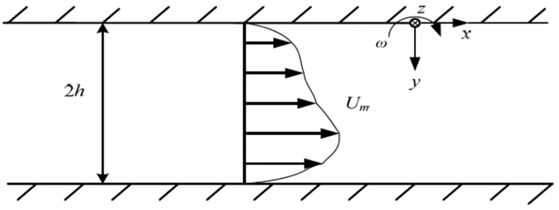
Figure 1. A sketch of the rotating channel flow. Extract from Huang’s study [52].
Jmse 10 02022 g001
Figure 2. The transient velocity with time at the center of the channel corresponds to the coordinates of (3.14, 1, 1) in the BADDES calculation results. (a) Total of about 334 flow cycles. (b) First 100 flow cycles.
Jmse 10 02022 g002
Figure 3. Comparison of mean velocity distribution with different turbulence models. DNS data from Yang et al. [51].
Jmse 10 02022 g003
Figure 4. Comparison of Reynolds stress components and the turbulent kinetic energy distribution with different turbulence models. DNS data from Yang et al. [51]. (a) Streamwise rms. (b) Normal direction rms. (c) Span direction rms. (d) Turbulent kinetic energy.
Jmse 10 02022 g004
Figure 5. Comparison of the contour of the f d variable with different turbulence models. (a) BADDES. (b) ADDES. (c) DDESO.
Jmse 10 02022 g005aJmse 10 02022 g005b
Figure 6. Transient fluctuation velocity distributions near the wall with different turbulence models at y/h = 0.04. (a) BADDES. (b) ADDES. (c) BkO. (d) DDESO.
Jmse 10 02022 g006
Figure 7. Transient fluctuation velocity distributions near the wall with different turbulence models at y/h = 1.96. (a) BADDES. (b) ADDES. (c) BkO. (d) DDESO.
Jmse 10 02022 g007
Figure 8. The isosurface at a certain time when the turbulence is fully developed with different turbulence models. The isosurface of Q is colored using the magnitude of the mean flow velocity. (a) BADDES, Q = 0.0025 s−2. (b) ADDES, Q = 0.0025 s−2. (c) BkO, Q = 0.0025 s−2. (d) DDESO, Q = 0.0003 s−2.
Jmse 10 02022 g008aJmse 10 02022 g008b
Figure 9. Sketch of the Taylor-Couette flow.
Jmse 10 02022 g009
Figure 10. Comparison of mean azimuthal velocity and mean angular momentum with different turbulence models. DNS data from Dong [54]. (a) Mean azimuthal velocity. (b) Mean angular momentum.
Jmse 10 02022 g010
Figure 11. Comparison of RMS fluctuation velocity and turbulent kinetic energy profiles of different models. The DNS results of the circumferential RMS fluctuation velocity from Dong [54] and other DNS results of the RMS fluctuation velocity are extracted from the study by Chouippe et al. [58]. (a) RMS azimuthal fluctuation velocity. (b) RMS radial fluctuation velocity. (c) RMS axial fluctuation velocity. (d) Turbulent kinetic energy.
Jmse 10 02022 g011
Figure 12. Comparison of the contour of the f d variable with different turbulence models. (a) BADDES. (b) ADDES. (c) DDESO.
Jmse 10 02022 g012
Figure 13. The expansion diagram of the instantaneous wall shear stress distribution on the inner cylindrical wall with different turbulence models. (a) BADDES, (b) ADDES, (c) BkO, and (d) DDESO.
Jmse 10 02022 g013
Figure 14. The expansion diagram of the instantaneous wall shear stress distribution on the outer cylindrical wall with different turbulence models. (a) BADDES, (b) ADDES, (c) BkO, and (d) DDESO.
Jmse 10 02022 g014
Figure 15. Sketch of swirling flow through an abrupt axisymmetric expansion.
Jmse 10 02022 g015
Figure 16. Schematic diagram of the grid used in the swirling flow through an abrupt expansion. (a) Grid distribution in the whole computing domain. (b) Grid distribution in the sudden expansion position. (c) Cross-section grid.
Jmse 10 02022 g016
Figure 17. Radial distributions of circumferential mean velocity, circumferential RMS velocity, mean axial velocity, and axial RMS velocity downstream of the expansion. Experimental data are from Foroutan and Yavuzkurt [60]. Jmse 10 02022 i001.
Jmse 10 02022 g017
Figure 18. Contour plots of the f d variable with different turbulence models (a) BADDES, (b) ADDES, and (c) DDESO.
Jmse 10 02022 g018
Figure 19. Contour plots of the transient axial velocity of different turbulence models on the meridian plane. The contour levels are between −0.4 and 0.8 at intervals of 0.05. (a) BADDES, (b) ADDES, (c) BkO, and (d) DDESO.
Jmse 10 02022 g019aJmse 10 02022 g019b
Figure 20. Iso-surface of Q = 1200 s−2 at a certain time when the turbulence is fully developed with different turbulence models. The iso-surface of the Q is colored using the transient axial velocity. The background is the average pressure distribution on the meridian plane. (a) BADDES, (b) ADDES, (c) BkO, and (d) DDESO.
Jmse 10 02022 g020
Table 1. Average time for iteration with different turbulence models.
Turbulence ModelCase1 (s)Case2 (s)Case3 (s)Average (s)Deviation (%)
BADDES0.24350.2450.2450.2445
ADDES0.2490.2470.2600.252+3.07
BkO0.2690.2740.2750.273+11.66
DDESO0.2730.2720.2710.272+11.25
Table 2. Relative errors of the RMS velocity were calculated by different models in the Taylor-Couette flow. (%).
Turbulence Model < u u > < v v > < w w > Average (s)
BADDES16.765.0214.1111.96
ADDES14.2617.2720.317.28
BkO14.2912.320.2315.61
DDESO46.7862.760.9756.82
Table 3. Average time for iteration with different turbulence models in the Taylor-Couette flow.
Turbulence ModelCase1 (s)Case2 (s)Case3 (s)Average (s)Deviation (%)
BADDES0.1770.1790.1710.1757
ADDES0.3550.3490.3570.3537+101.33
BkO0.1910.1880.1920.1903+8.35
DDESO0.370.360.3580.3627+106.45
Table 4. Average time for iteration with different turbulence models in the swirling flow through an abrupt axisymmetric expansion.
Turbulence ModelCase1 (s)Case2 (s)Case3 (s)Average (s)Deviation (%)
BADDES0.4080.4070.4000.405
ADDES0.40.4110.4250.412+1.728
BkO0.4840.4240.460.456+12.593
DDESO0.3690.4130.3670.383−5.432
Publisher’s Note: MDPI stays neutral with regard to jurisdictional claims in published maps and institutional affiliations.