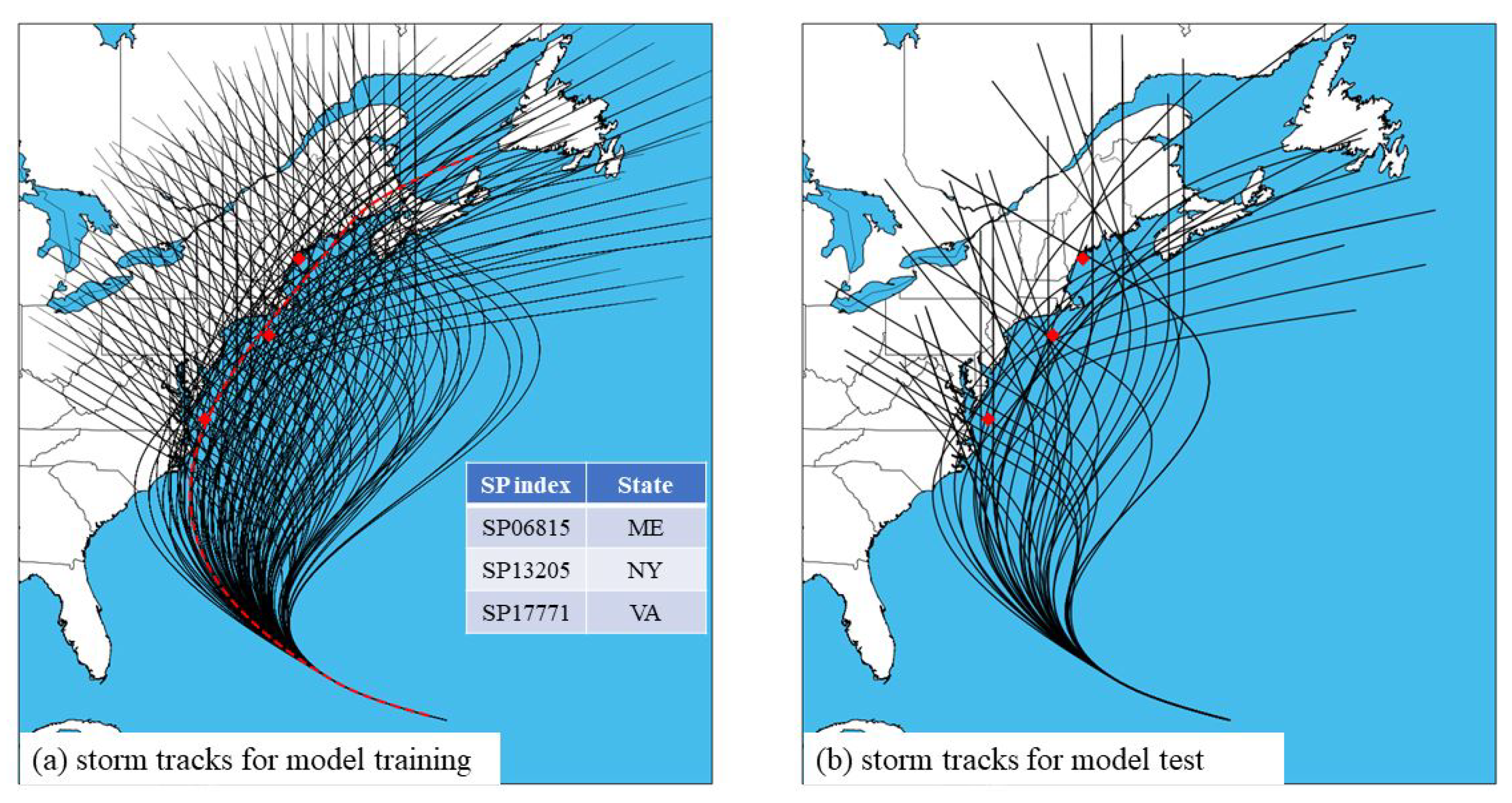
Figure 1.
The synthetic storm tracks used by the NACCS storm surge dataset. In total, 1031 storm tracks were randomly divided into two groups: (
a) The first group of 981 storms was used to train the neural network storm surge forecast model, and (
b) the second group of 50 storms was used to test the trained model. Three save points where storm surge forecast models developed in this work are indicated in a diamond marker. The red dashed line in subplot (
a) indicates a training storm analyzed in
Figure 3 and
Figure 4.
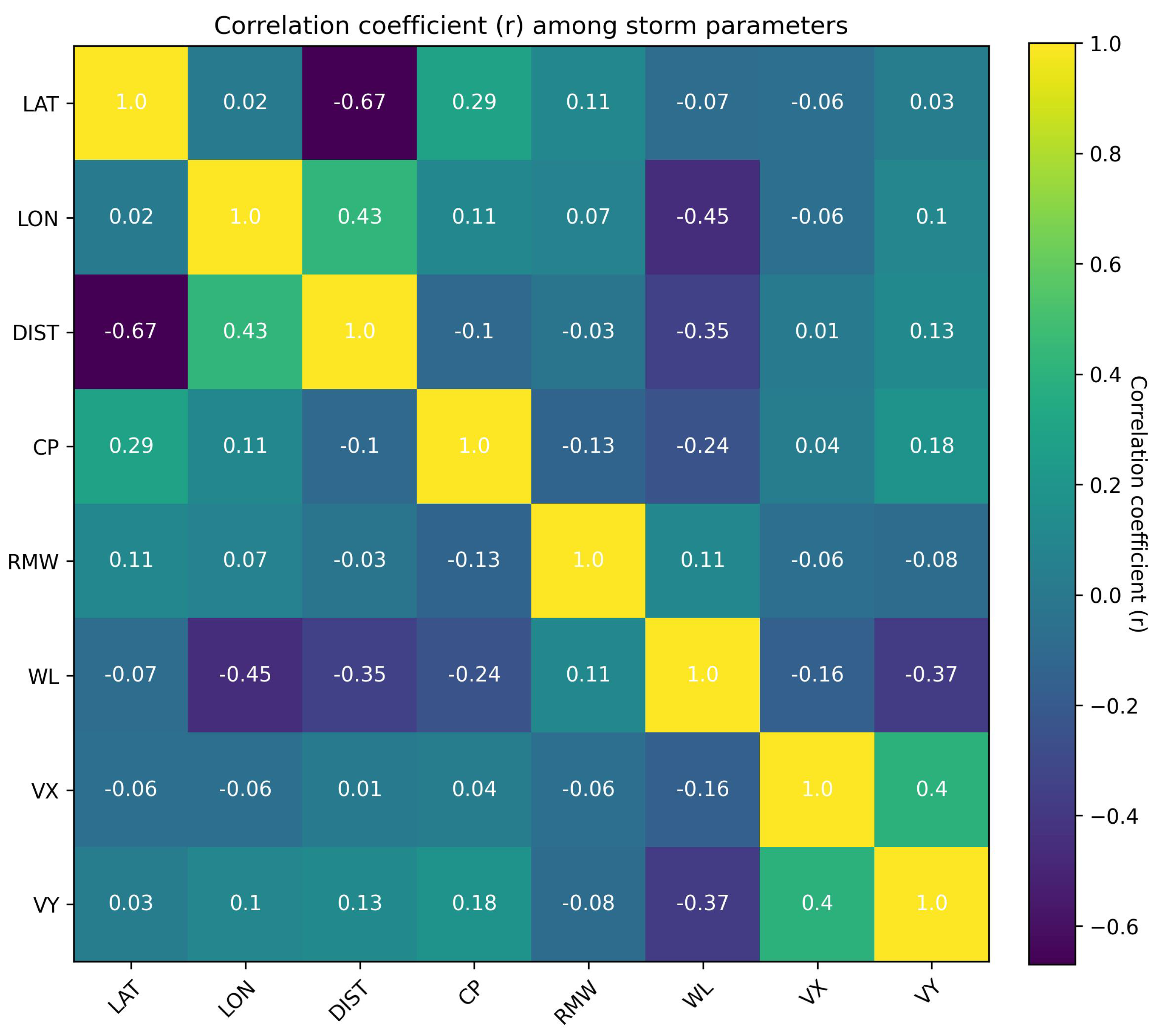
Figure 2.
The Pearson standard correlation coefficient among storm parameters used to develop storm surge forecast model. LAT: latitude of storm center; LON: longitude of storm center; DIST: Distance between storm center and save point; CP: Central pressure of a storm; RMW: radius of the maximum winds; WL: storm surge water level; VX: storm−induced velocity in the x direction, and VY: storm−induced velocity in the y direction.
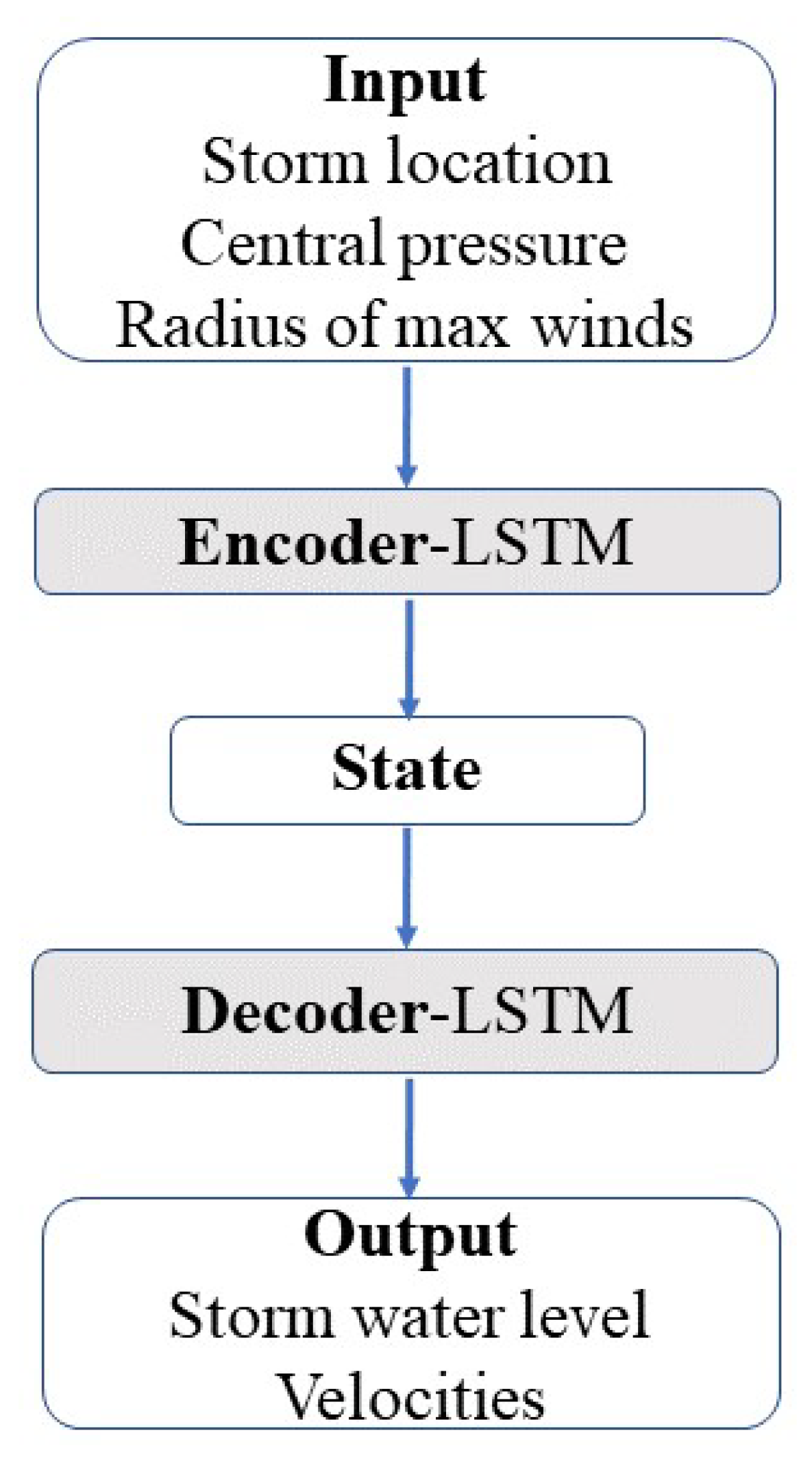
Figure 5.
The encoder–decoder neural network framework for storm surge forecast. The encoder layer encodes the input into an internal state, and then the decoder layer decodes the internal state to the output. The input includes the storm center (longitude and latitude), the central pressure, and the radius of maximum winds, and the output includes storm-induced water level and velocity in the x and y directions. The LSTM model, a recurrent neural network, was used as the encoder and the decoder.
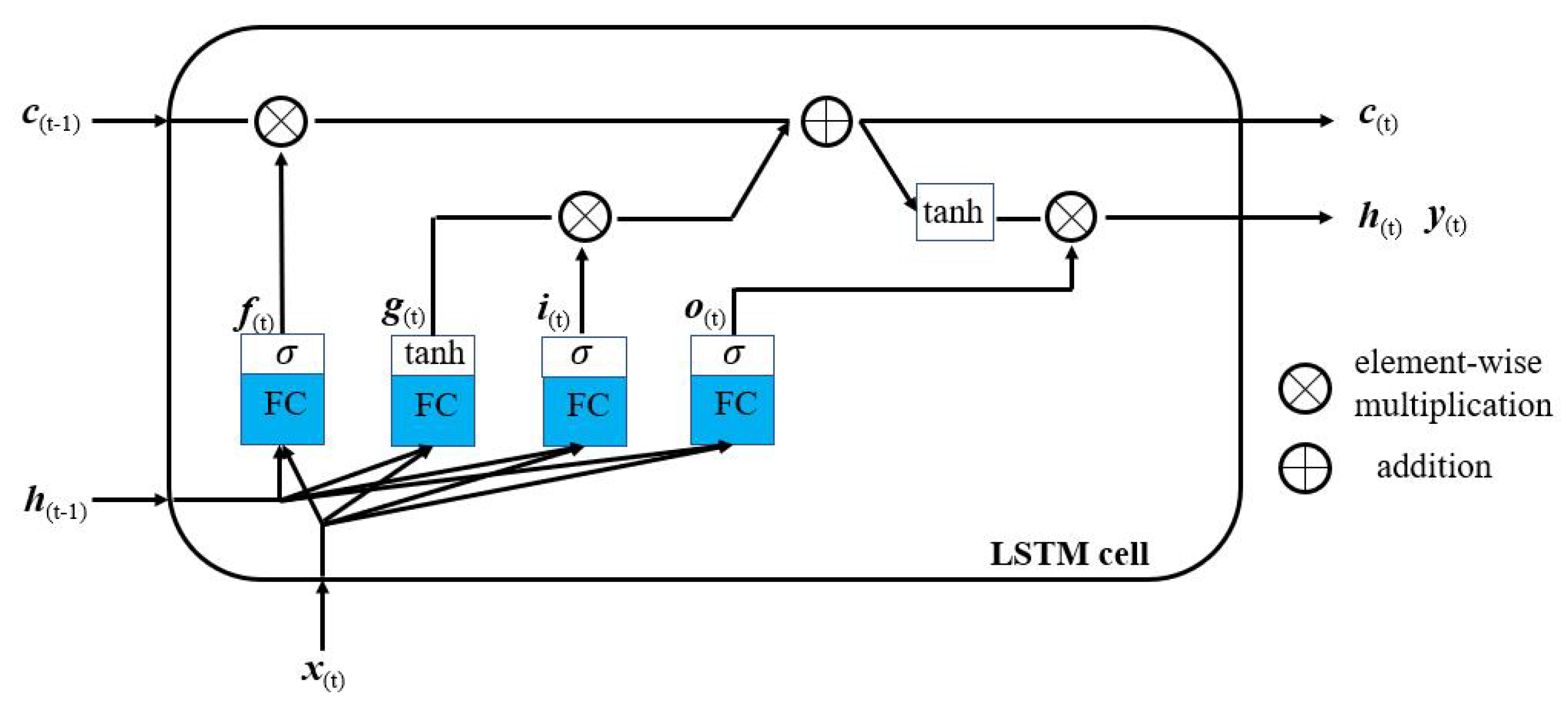
Figure 6.
Sketch of the LSTM cell network diagram (after [
22]).
Figure 6.
Sketch of the LSTM cell network diagram (after [
22]).
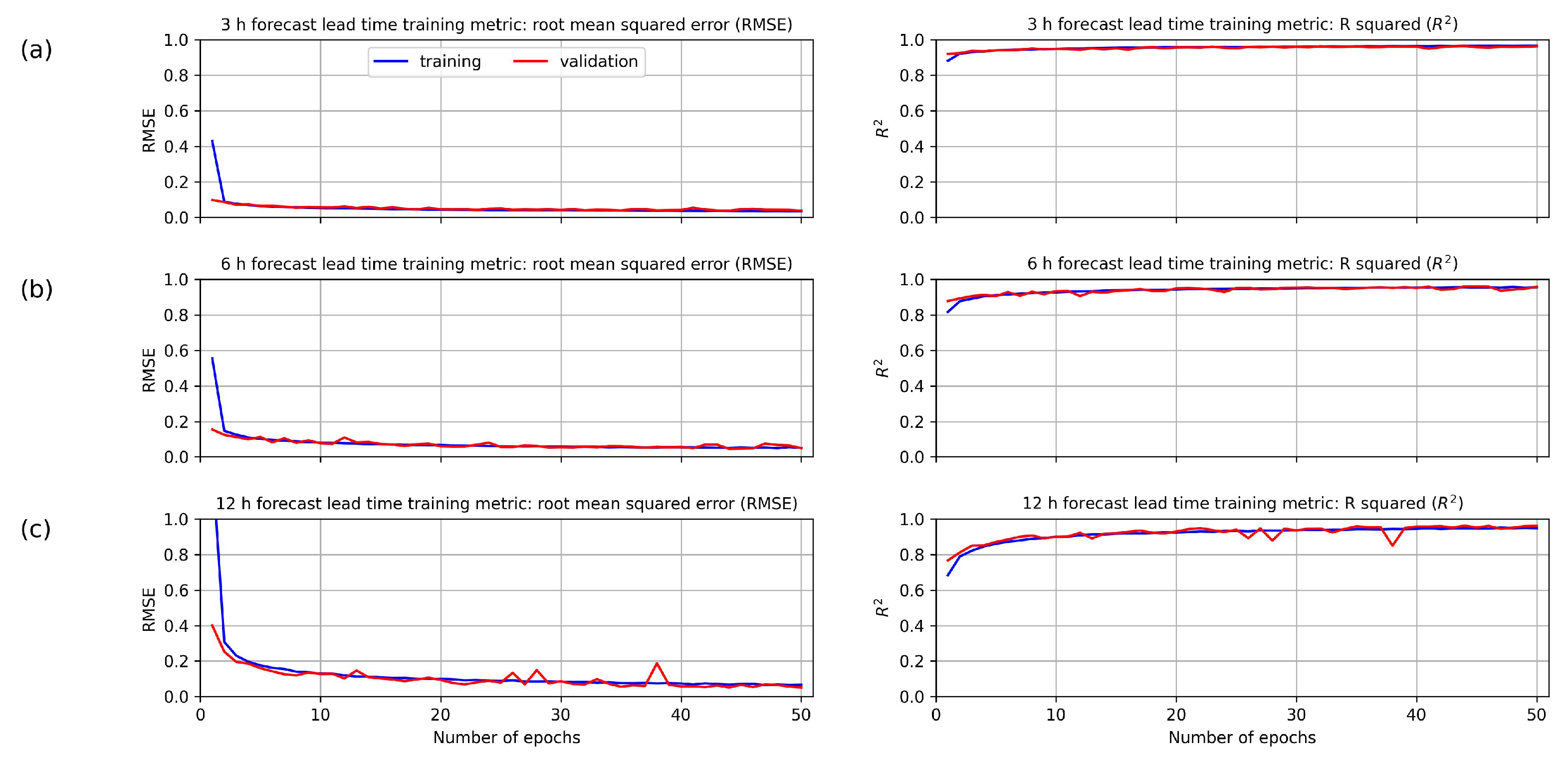
Figure 7.
The neural network model training metrics for three forecast lead times (i.e., 3 h, 6 h, and 12 h) from (a–c) for save point SP13205. Two metrics, root mean square error (RMSE) and R squared (), were used.
Figure 7.
The neural network model training metrics for three forecast lead times (i.e., 3 h, 6 h, and 12 h) from (a–c) for save point SP13205. Two metrics, root mean square error (RMSE) and R squared (), were used.
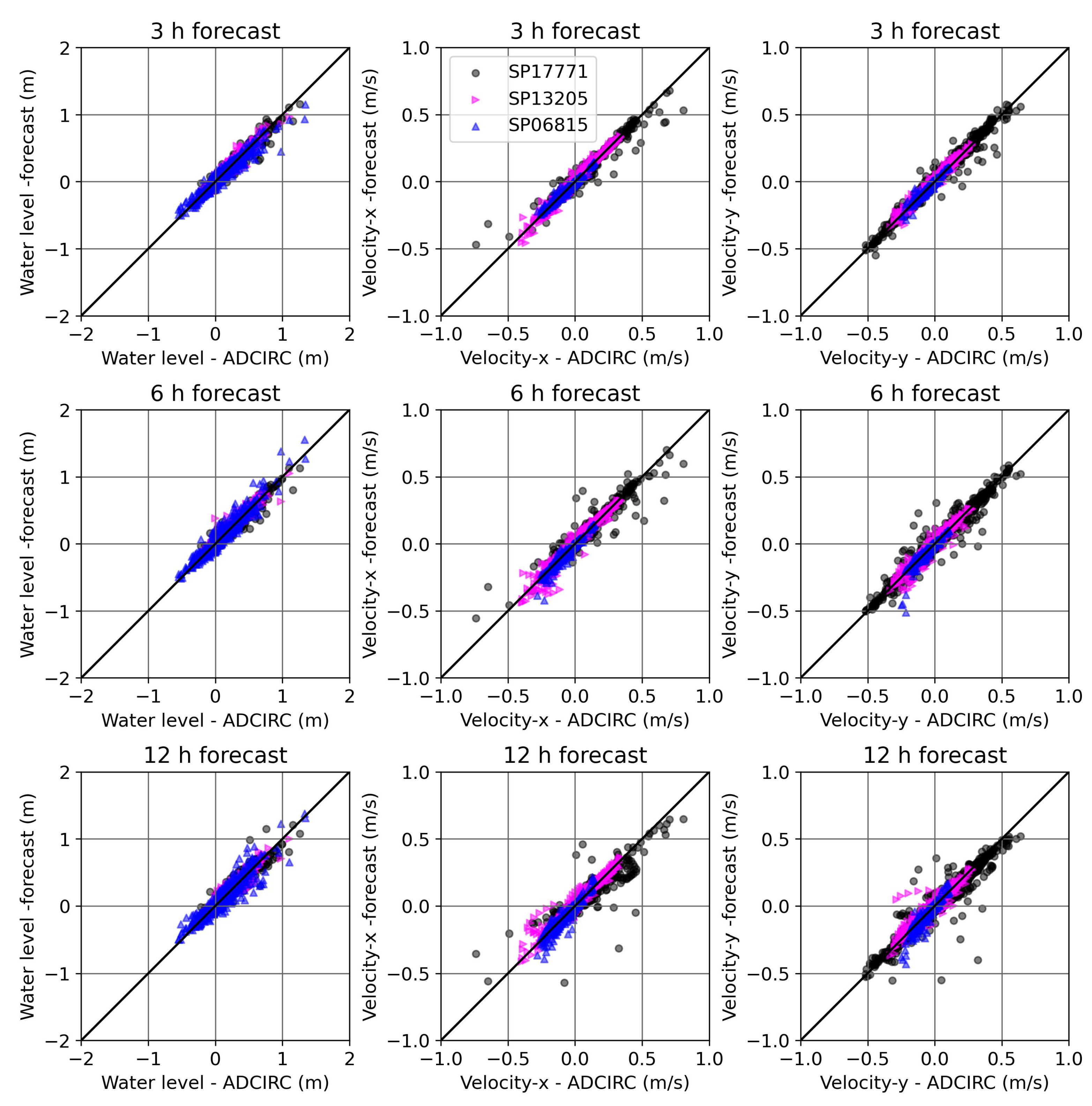
Figure 8.
Scatter plot comparison of storm surge water level (left column), velocity in the x-direction (middle column), and velocity in the y-direction (right column) between neural network storm surge forecast model and ADCIRC simulation at three save points using three different forecast lead times (i.e., 3 h, 6 h, and 12 h) from top to bottom rows. SP17771: dots; SP13205: right arrows; and SP06815: upper arrows.
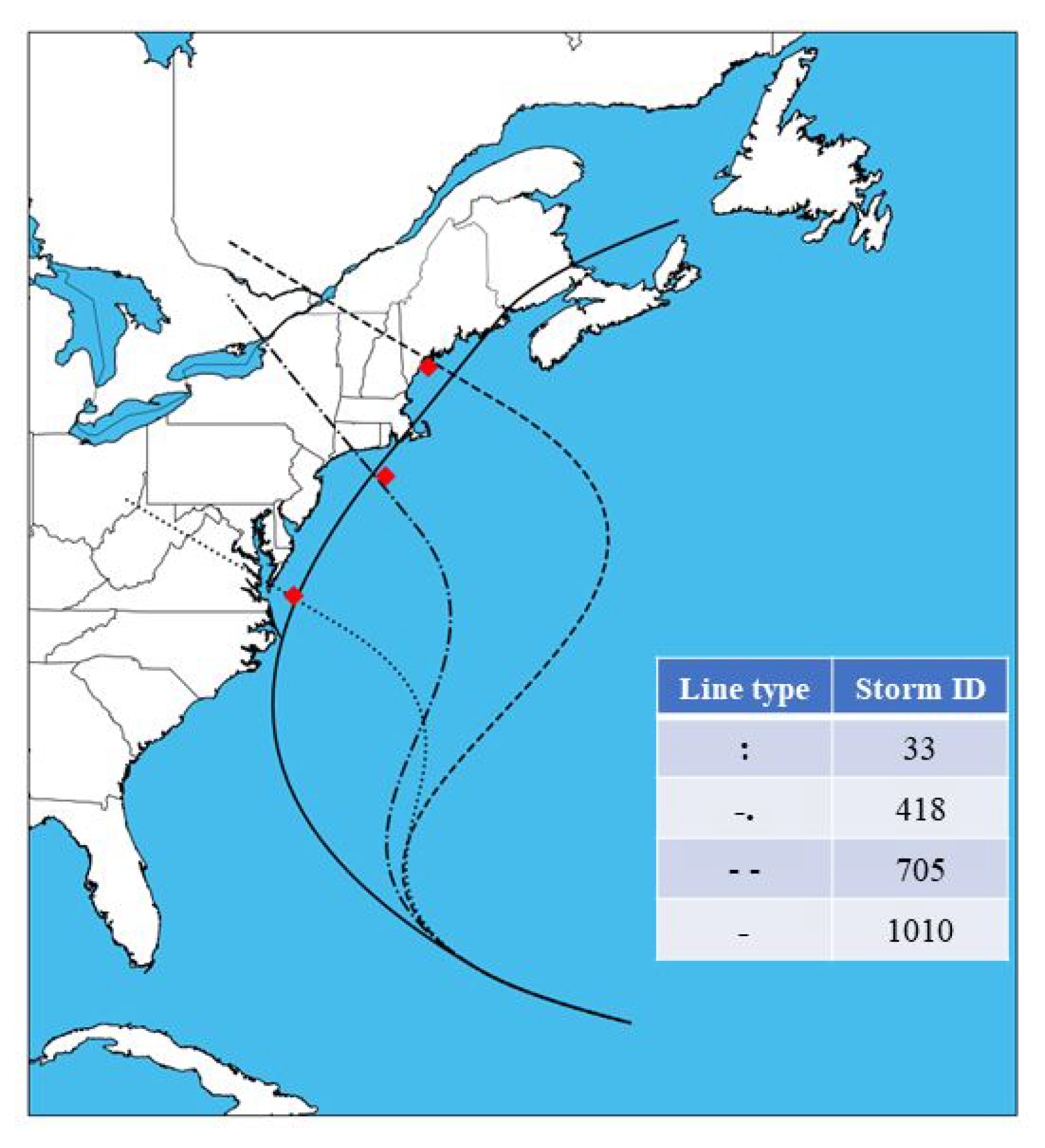
Figure 9.
The selected bypassing storm 1010 and three landfalling storms 33, 418, and 705 for evaluating the neural network storm surge forecast model. The diamond symbol indicates three save points, and their index can be found in
Figure 1.
Figure 9.
The selected bypassing storm 1010 and three landfalling storms 33, 418, and 705 for evaluating the neural network storm surge forecast model. The diamond symbol indicates three save points, and their index can be found in
Figure 1.
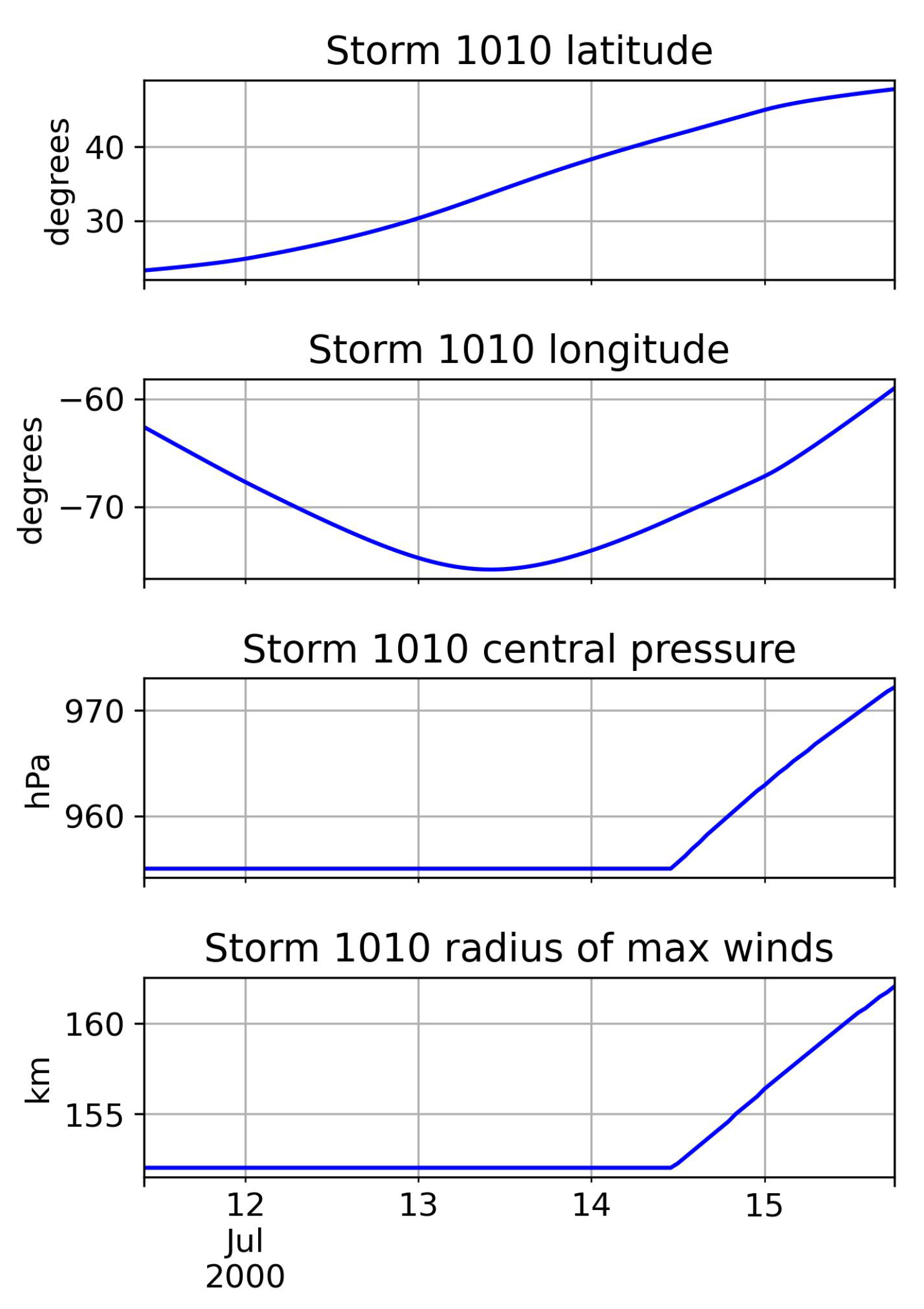
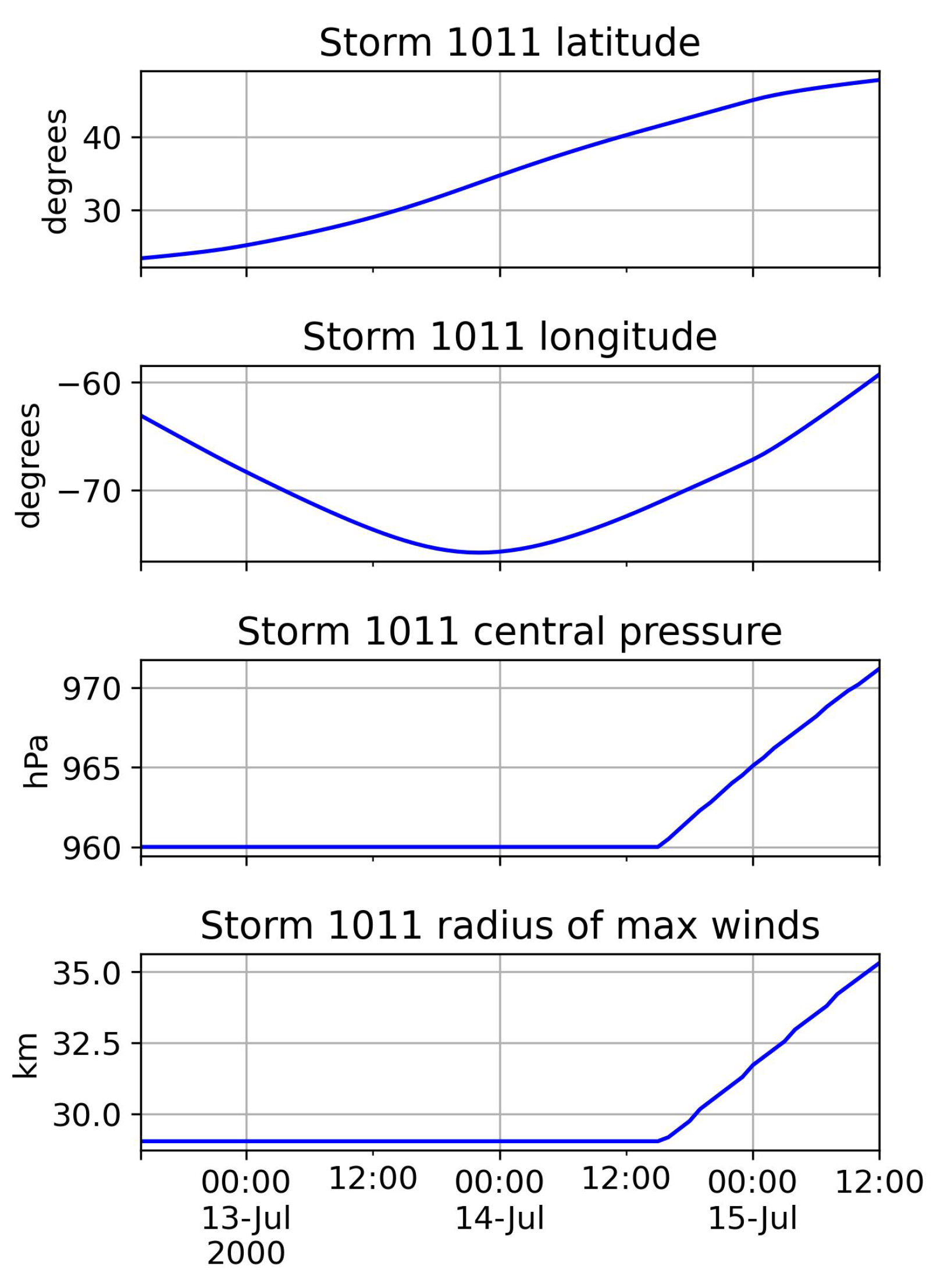
Figure 10.
The time-series profiles of storm center (i.e., longitude and latitude), the central pressure, and the radius of the maximum winds of the bypassing storm 1010.
Figure 10.
The time-series profiles of storm center (i.e., longitude and latitude), the central pressure, and the radius of the maximum winds of the bypassing storm 1010.
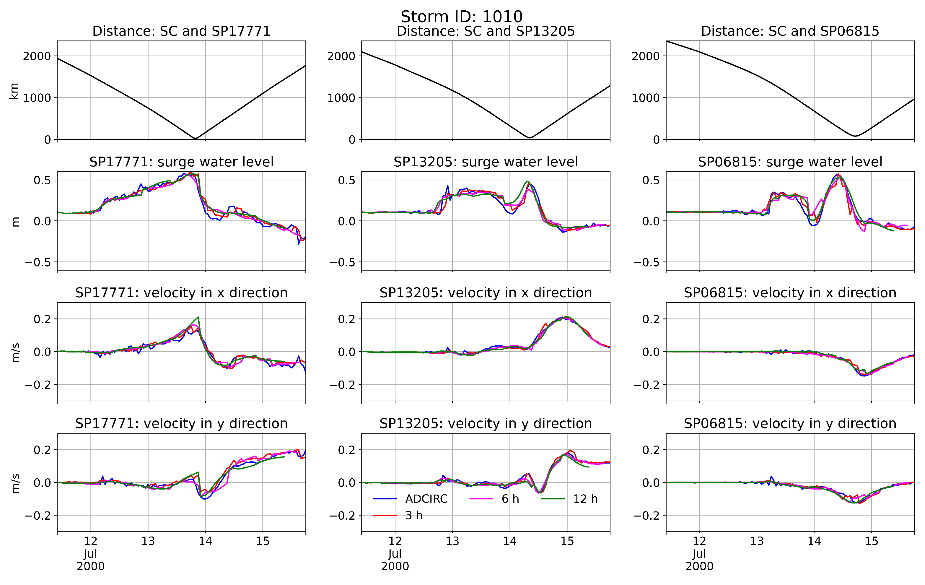
Figure 11.
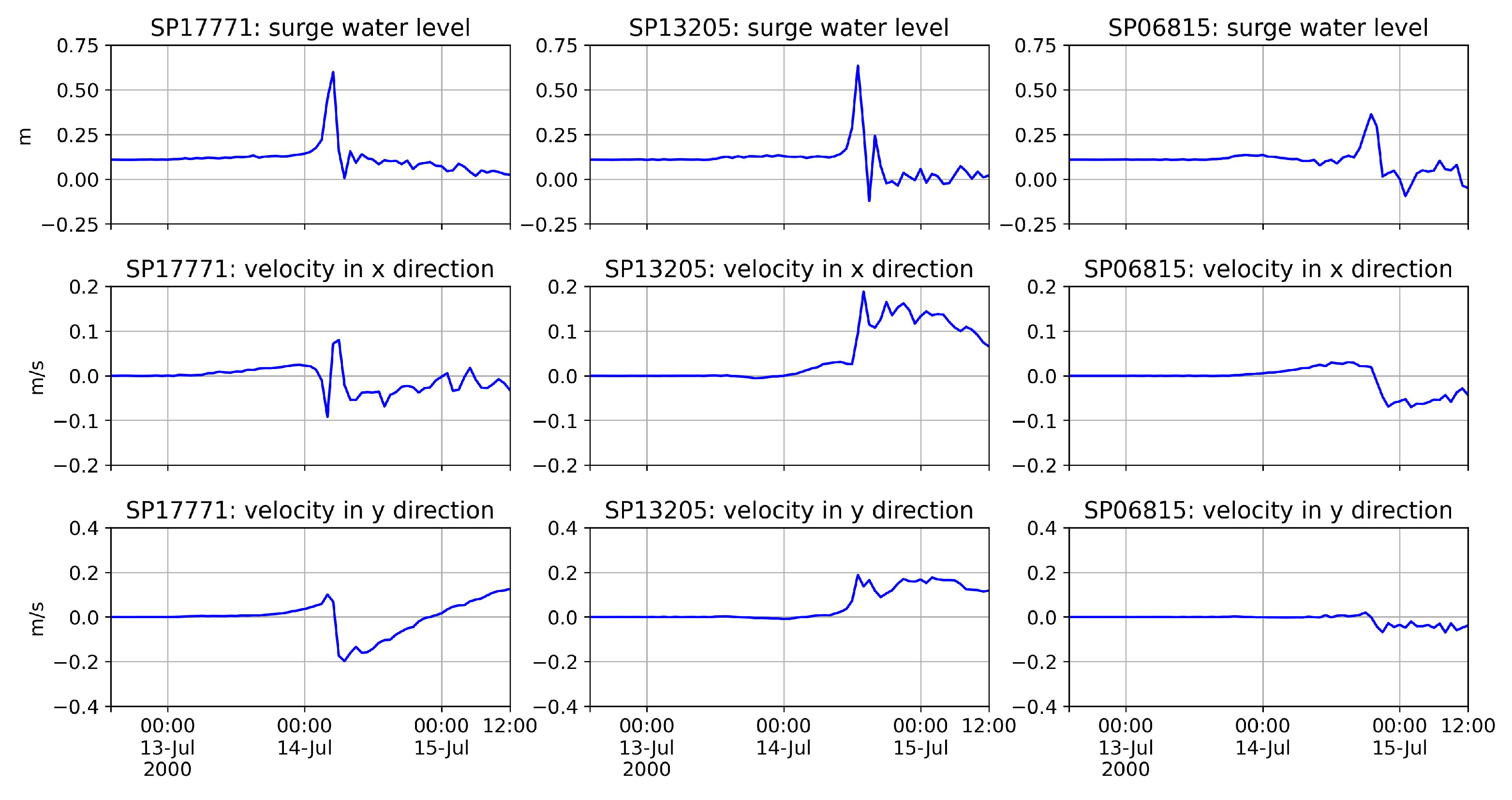
Comparison of storm surge water level and velocity induced by the bypassing storm 1010 at three save points. Forecasts using three lead times (i.e., 3 h, 6 h, and 12 h) were compared with ADCIRC simulation. The top row is the distance between the storm center and the save point; the second row, counting from top to bottom, is the surge water level, and the bottom two rows are storm-induced velocities in x and y directions, respectively.
Figure 11.
Comparison of storm surge water level and velocity induced by the bypassing storm 1010 at three save points. Forecasts using three lead times (i.e., 3 h, 6 h, and 12 h) were compared with ADCIRC simulation. The top row is the distance between the storm center and the save point; the second row, counting from top to bottom, is the surge water level, and the bottom two rows are storm-induced velocities in x and y directions, respectively.
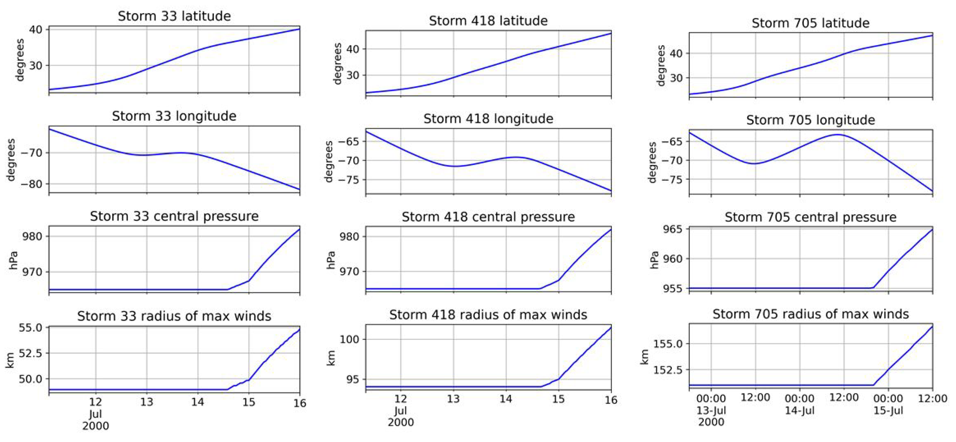
Figure 12.
The time-series profiles of storm center (i.e., longitude and latitude), central pressure, and the radius of the maximum winds of the landfalling storms 33 (left), 418 (middle), and 705 (right).
Figure 12.
The time-series profiles of storm center (i.e., longitude and latitude), central pressure, and the radius of the maximum winds of the landfalling storms 33 (left), 418 (middle), and 705 (right).
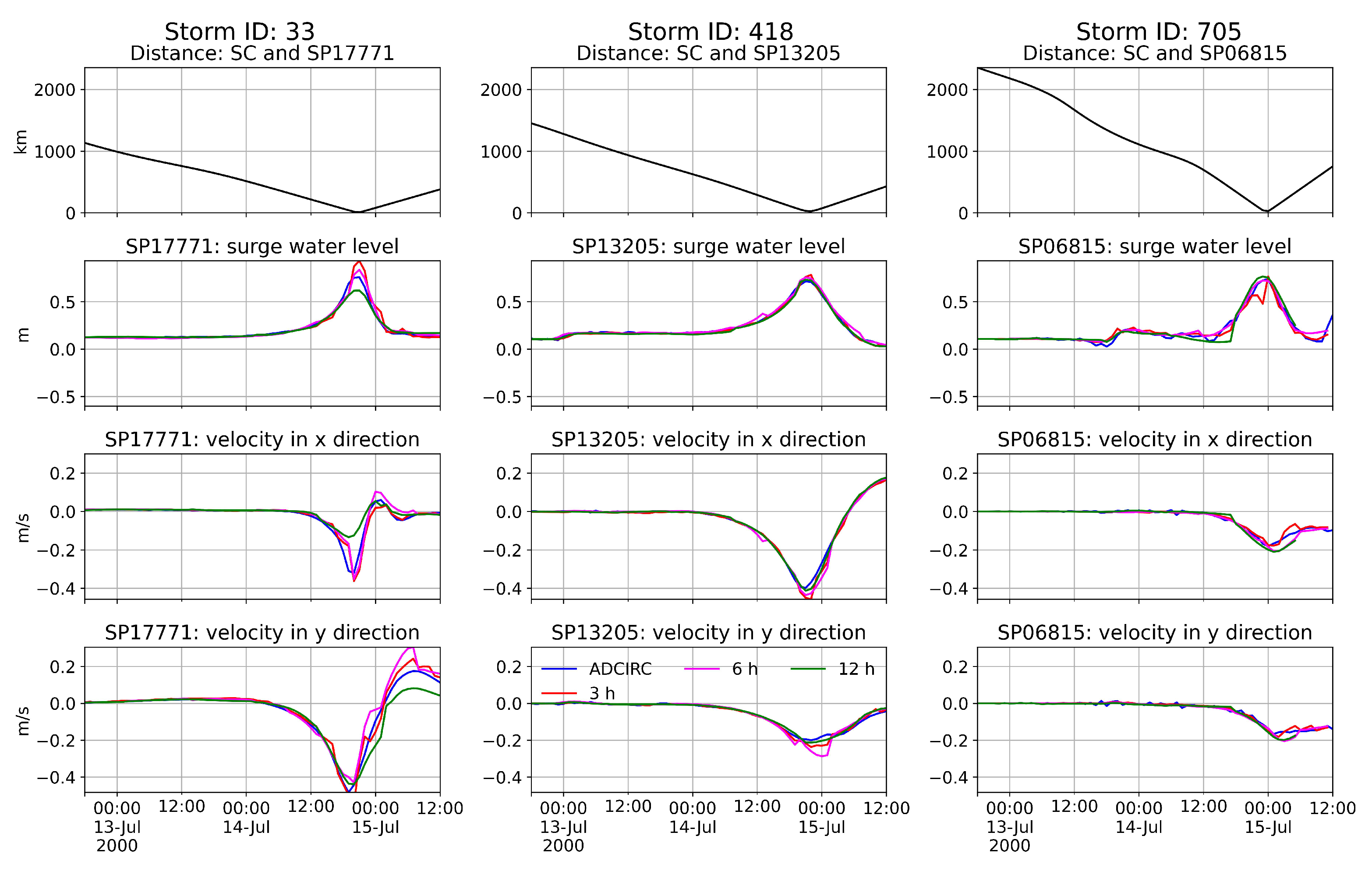
Figure 13.
Comparison of storm surge water level and velocity induced by the landfalling storms 33, 418, and 705 at three save points SP17771, SP13205, and SP06815, respectively. Forecast using three lead times (i.e., 3 h, 6 h, and 12 h) were compared with ADCIRC simulation.
Figure 13.
Comparison of storm surge water level and velocity induced by the landfalling storms 33, 418, and 705 at three save points SP17771, SP13205, and SP06815, respectively. Forecast using three lead times (i.e., 3 h, 6 h, and 12 h) were compared with ADCIRC simulation.
Table 1.
The index number, water depth, and location information for the selected three save points in the NACCS storm surge dataset.
Table 1.
The index number, water depth, and location information for the selected three save points in the NACCS storm surge dataset.
| Save Points | Water Depth (m) | State | Location (Lat, Lon) |
|---|
| SP17771 | 40.0 | Virginia | 37.061 N 75.048 W |
| SP13205 | 74.0 | New York | 40.537 N 71.606 W |
| SP06815 | 60.7 | Maine | 43.580 N 70.000 W |
Table 2.
The definitions of parameters used for storm surge forecast model development.
Table 2.
The definitions of parameters used for storm surge forecast model development.
| Variables | Description |
|---|
| Latitude (deg) | The latitude of the storm center |
| Longitude (deg) | The longitude of the storm center |
| Central pressure (hPa) | The pressure in the center of the storm. |
| Radius of maximum winds (km) | The radius to the maximum wind from the storm center. |
| Water level (m) | Storm induced water level. |
| X-velocity (m/s) | Storm-induced depth-averaged velocity in the x direction. |
| Y-velocity (m/s) | Storm-induced depth-averaged velocity in the y direction. |
Table 3.
Summary of the proposed encoder–decoder storm surge forecast model with a lead time of 6 h. The first column is the layer index, the second is the layer type, the third is the output shape of each layer, and the fourth is the number of training parameters.
Table 3.
Summary of the proposed encoder–decoder storm surge forecast model with a lead time of 6 h. The first column is the layer index, the second is the layer type, the third is the output shape of each layer, and the fourth is the number of training parameters.
| Layer # | Layer Type | Output Shape | # of Parameters |
|---|
| 1 | InputLayer | (none, 6, 8) | 0 |
| 2 | LSTM | (none, 50) | 12,200 |
| 3 | Flatten | (none, 50) | 0 |
| 4 | RepeatVector | (none, 6, 50) | 0 |
| 5 | LSTM | (none, 6, 50) | 20,200 |
| 6 | Dense | (none, 6, 50) | 2550 |
| 7 | Dense | (none, 6, 3) | 153 |
Table 4.
The average computation time to train the neural network model for 50 epochs and the computation time to run the neural network model for 50 test storms using three forecast lead times (i.e., 3 h, 6 h, and 12 h).
Table 4.
The average computation time to train the neural network model for 50 epochs and the computation time to run the neural network model for 50 test storms using three forecast lead times (i.e., 3 h, 6 h, and 12 h).
| Forecast Lead Time (h) | Model Training Time (s) | Model Test Time (s) |
|---|
| 3 | 1275.38 | 78.55 |
| 6 | 1897.52 | 36.05 |
| 12 | 2625.88 | 18.43 |
Table 5.
Summary of root mean squared error (RMSE) between neural network forecast and ADCIRC simulation for water level (WL) in meters, velocity in the x direction (VX) in m/s, and velocity in the y direction (VY) in m/s for three save points using three forecast lead times (i.e., 3 h, 6 h, and 12 h) using 50 test storms.
| | 3 h | 6 h | 12 h |
|---|
| SP17771 | WL | 0.024 | 0.026 | 0.029 |
| VX | 0.017 | 0.021 | 0.029 |
| VY | 0.018 | 0.022 | 0.032 |
| SP13205 | WL | 0.021 | 0.023 | 0.025 |
| VX | 0.009 | 0.013 | 0.014 |
| VY | 0.009 | 0.012 | 0.016 |
| SP06815 | WL | 0.029 | 0.033 | 0.039 |
| VX | 0.006 | 0.008 | 0.011 |
| VY | 0.006 | 0.010 | 0.011 |
Table 6.
Summary of R squared () between neural network forecast and ADCIRC simulation for water level (WL), velocity in the x direction (VX), and velocity in the y direction (VY) for three save points for three forecast lead times (i.e., 3 h, 6 h, and 12 h) using 50 test storms.
Table 6.
Summary of R squared () between neural network forecast and ADCIRC simulation for water level (WL), velocity in the x direction (VX), and velocity in the y direction (VY) for three save points for three forecast lead times (i.e., 3 h, 6 h, and 12 h) using 50 test storms.
| | 3 h | 6 h | 12 h |
|---|
| SP17771 | WL | 0.97 | 0.96 | 0.95 |
| VX | 0.95 | 0.92 | 0.85 |
| VY | 0.98 | 0.96 | 0.93 |
| SP13205 | WL | 0.97 | 0.96 | 0.96 |
| VX | 0.98 | 0.96 | 0.95 |
| VY | 0.97 | 0.95 | 0.90 |
| SP06815 | WL | 0.94 | 0.92 | 0.89 |
| VX | 0.98 | 0.97 | 0.94 |
| VY | 0.97 | 0.94 | 0.92 |
Table 7.
Four representative test storms for time-series storm surge analysis at three save points. There are one bypassing storm and three landfalling storms, with each making landfall near one save point.
Table 7.
Four representative test storms for time-series storm surge analysis at three save points. There are one bypassing storm and three landfalling storms, with each making landfall near one save point.
| Storm ID | Storm Type | Save Points |
|---|
| 1010 | Bypassing | SP17771, SP13205, SP06815 |
| 33 | Landfalling | SP17771 |
| 418 | Landfalling | SP13205 |
| 705 | Landfalling | SP06815 |


