A Deep Learning Method for NLOS Error Mitigation in Coastal Scenes

Abstract

With the widespread use of automatic identification systems (AISs), some ships use deceptive information or intentionally close their AISs to conceal their illegal activities or evade the supervision of maritime departments. Although radar measurements can be effectively utilized to evaluate the credibility of received AIS data, the propagation of non-line-of-sight (NLOS) signal conditions is an important factor that affects location accuracy. This study addresses the NLOS problem in a special geometric dilution of precision (GDOP) scenario on a coast and several base stations. We employed data augmentation and a deep residual shrinkage network in order to alleviate the adverse effects of NLOS errors. The results of our simulations demonstrate that the proposed method outperforms other range-based localization algorithms in a mixed LOS/NLOS environment. For a special GDOP scenario with four radars, our algorithm’s root-mean-square error (RMSE) was lower than 180 m.

1. Introduction

AISs have been widely adopted in the maritime field in order to monitor marine traffic and avoid vessel collisions [1]. However, some ships do not maintain their AISs in a normal working state, or they input fraudulent information into their equipment. As a result, AIS signals cannot be effectively received by other vessels and land services, which directly threatens the safety of water traffic. This leads to a myriad of problems in maritime surveillance, including unauthorized maritime arrivals, illegal or unregulated fishing and immigration, smuggling, pollution, piracy, and maritime terrorism.

Over the last decade, interest in identifying the credibility of received AIS data has increased. As shown in [2], Katsilieris adopted radar measurement information to evaluate the dependability of AIS data. Their study assumed that the radar system worked in an LOS environment. However, due to the lack of an NLOS path, signals can only reach the receiver via direct penetration, reflection, diffraction, and scattering [3,4,5]. The propagation of NLOS conditions creates a positive bias in distance measurements, which significantly affects the positioning accuracy. Direct and post-identification mitigation are two common methods for handling NLOS errors. In the former, NLOS errors can be mitigated by processing the measurement information [6,7,8,9,10,11,12,13,14]. In contrast, the method of post-identification reduces the errors by identifying NLOS base stations (BSs) [15,16,17,18,19,20]. However, most previous studies were based on cellular networks and assumed that the target was within a polygon of sufficient BSs that had GDOP conditions. At present, there are few reports concerning the location problem with insufficient BSs and more serious NLOS propagation in special GDOP scenarios on a coast.

In this paper, we adopt an original method of comparing positions and AIS tracks in order to identify ships with abnormal AIS signals, and this method is based on an efficient NLOS error mitigation scheme that employs data augmentation and a deep residual shrinkage network (DRSN). The data enhancement method generates multiple positioning features by grouping prepositioning features. First, the original distance data are grouped according to the BSs. Subsequently, a traditional mathematical model is used for the preliminary positioning of each group of distance data to generate the preliminary positioning characteristics. As a feature-learning method for strong noise and highly redundant data, the DRSN can effectively identify NLOS features after data enhancement. The NLOS error mitigation scheme can be divided into four phases: elimination of antenna delay, grouping locations, dataset construction, and DRSN positioning model training. The radar measurement information is converted into image data after data enhancement by eliminating the antenna delay, grouping position, and dataset construction. Finally, a classic DRSN model, Densenet, is used to calculate the target’s location. The key contributions of this study are as follows.

(1) We developed of an efficient NLOS error mitigation scheme based on a DRSN in order to mitigate NLOS errors in special GDOP scenarios with fewer BSs.

(2) We developed a preliminary location grouping method that allows the DRSN model to identify the features of NLOS BSs.

(3) Several simulations were performed in mixed LOS/NLOS environments. The numerical results show that the proposed method’s performance is highly competitive with that of previous methods.

This paper is organized as follows: The next section presents several prior studies in this field. Section 3 demonstrates the model of the localization system and the effect of the GDOP on location accuracy. Section 4 presents the design of the NLOS error mitigation scheme based on the DRSN. In Section 5, we introduce the experimental process, compare the performance, and analyze the positioning error. Section 6 concludes the paper.

2. Related Work

There are two approaches to the propagation of signal NLOS scenarios: direct and post-identification mitigation. The former attenuates NLOS errors by processing measurement information directly [6,7,8,9,10,11,12,13,14]. In contrast, the post-identification method identifies NLOS BSs by using different propagation characteristics in LOS and NLOS environments. The error of NOLS is then reduced by eliminating NLOS data or through other methods [15,16,17,18,19,20].

The direct mitigation method achieves higher performance in the case of small NLOS errors. These errors were mitigated by using the maximum likelihood (ML) algorithm in [6]. In [7,8], the NLOS error problem was converted into a quadratic programming problem, and the influence of the NLOS error was mitigated by the extremum of the objective function. In [9], a residual weighting algorithm (RWGH) was proposed to locate the source accurately without requiring the NLOS status in advance. This algorithm first calculated one positioning result for each combination of three or more distance measurements. Then, distance data were obtained by submitting the coordinates to the positioning equation. The final positioning coordinates were then obtained by weighting all combinations of results. The authors of [10] improved the residual weighting algorithm by combining the TOA and AOA to locate a target based on two BSs. The authors of [11] used the iterative minimum residual (IMR) to obtain a suboptimal solution. In [12], Wang described the TDOA-based source positioning problem as a robust least squares (RLS) problem, and they sought robust position estimation for NLOS errors. In addition, positioning technology based on semidefinite programming (SDP) was proposed in [13]. Su proposed a method for converting a TDOA model into a TOA model. After mathematical modeling was applied in order to express the localization problem as a semidefinite programming problem, a semidefinite programming solver was used to solve it. The authors of [14] proposed a combination of the square range (SR) and weighted least squares (WLS) methods in order to convert the initial non-convex problem into a generalized trust-region subproblem (GTRS) without prior knowledge of the bias. The solution could then be obtained with a bisection procedure. However, the direct mitigation algorithm exhibited poor performance when handling large NLOS errors or insufficient LOS BSs.

When the NLOS error is evident, we can identify whether specific measurement data contain NLOS errors. Accordingly, various methods can be used to reduce NLOS errors and improve positioning accuracy. In [15,16,17], based on the peak detection and channel model technology, these methods exhibited significantly higher accuracy than that of existing algorithms in the detection of NLOS paths. In [18], a fast algorithm was designed with the subspace method to identify NLOS errors by using the eigenvector (FINE) algorithm. However, in practical applications, the algorithm must be executed repeatedly to locate all NLOS paths, as only one NLOS path can be found in each run. The authors of [19,20] proposed a TOA-based localization scheme that locates a source by using a combination of three selected BSs in wireless sensor networks. Subsequently, the residual vector is computed from the initial positioning result of the selected BSs and the original observed values. This residual vector can be used to determine LOS and NLOS paths. However, the localization performance of these algorithms is limited because the observed NLOS values are discarded in the location estimation.

From the aforementioned studies, it is clear that NLOS mitigation in special scenarios has not been sufficiently researched. However, the scenario presented in this study exhibits a strong application background and practical value in engineering. Therefore, we adopted deep learning in order to improve the location performance under GDOP conditions with fewer BSs.

3. Preliminary

In this section, we introduce the model of the localization system and the effect of GDOP on the location accuracy.

3.1. Localization System Model

NLOS errors are caused by the lack of an LOS path between a BS and the target. Because propagation time in NLOS conditions is longer than that in LOS conditions, these errors always add a positive value to the true range. As shown in Figure 1, there are two BS signals—BS1 and BS7—that cannot be transmitted over the LOS path due to the presence of obstacles. BS1 receives signals through penetration, whereas BS7 receives signals through reflection. If the measured values of BS1 and BS7 were to be used in the positioning process, a significant positioning error would occur. However, in the cellular network scenario shown in Figure 1, although the signal propagation of BS1 and BS7 is classified as NLOS propagation, there are still five BSs that have LOS propagation paths. Therefore, we can still locate the target by using other LOS BSs or the residual method in order to minimize the influence of NLOS errors. However, these errors are difficult to eliminate in cases with fewer BSs.

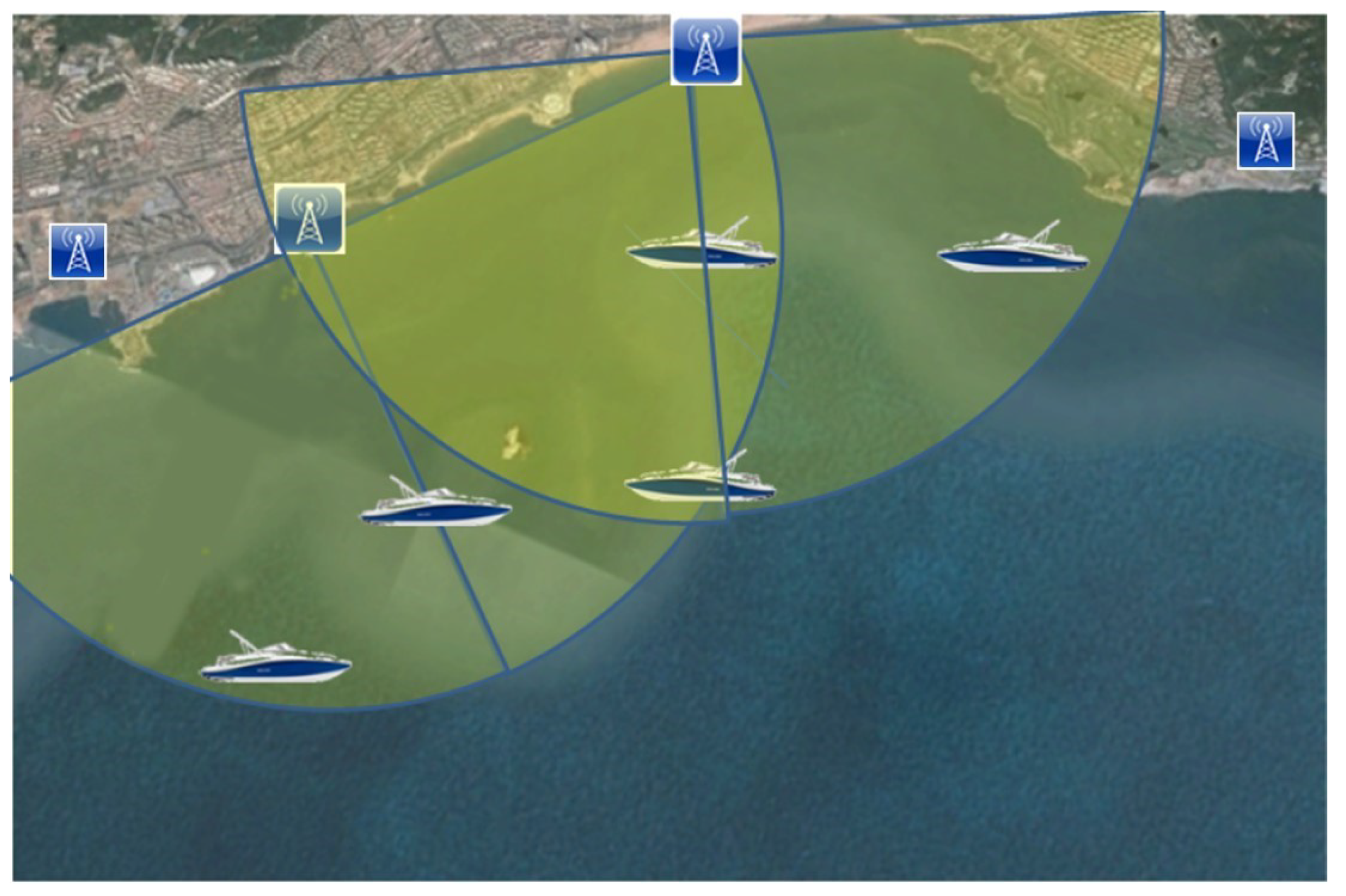
As shown in Figure 2, coastal scenarios generally include fewer BSs, and the target is outside the BS polygon. When the number of LOS BSs is relatively small, it is difficult to compensate for NLOS errors, which adversely affects the positioning accuracy. Therefore, this study largely focuses on minimizing the effects of NLOS errors.

Measurement and NLOS errors are the main factors affecting ranging accuracy. Generally, NLOS errors are significantly larger than measurement errors. Assuming that there are n BSs in a system, the measured range in the ith BS can be expressed by Equation (1):

$$\widetilde{d_i}=d_i+e_i+n_i,i=1,2,3\cdots ,n$$

(1)

where $\widetilde{d_i}$ is the actual measurement distance, and $d_i$ represents the true distance between the ith BS and the target. $e_i$ represents the measurement error, which follows Gaussian random variables with a mean at 0 and a variance of ${\sigma }^2$. $n_i$ denotes the NLOS error, which is assumed to be an independent and identically distributed uniform distribution between $0.05d_i$ and $0.9d_i$ [21].

3.2. Influence of the GDOP on Location Accuracy

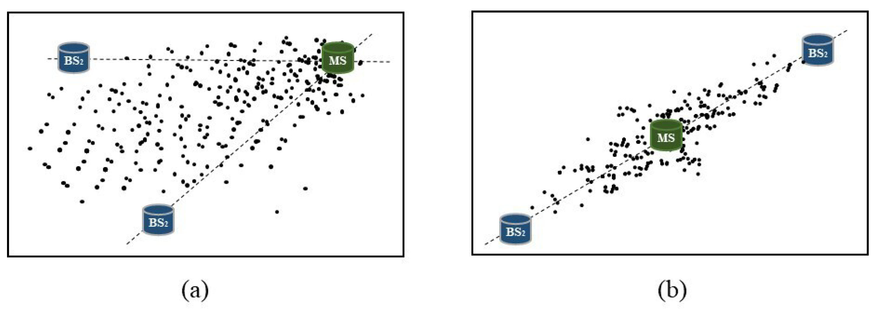
The GDOP, which refers to the relationship between the geometric positions of a BS and the target, is an important factor that affects location accuracy. In [22], for four BSs arranged in a circle, the positioning accuracy was least affected when the target was at the circle’s center. When the target was outside the circle, the GDOP rapidly increased. The authors of [23] conducted comparative experiments under different GDOP scenarios. In the case of two NLOS BSs in the same direction, the range of position estimation results was large, as shown in Figure 3a. For NLOS BSs in the opposite direction, as shown in Figure 3b, the mean square error was significantly smaller than that shown in Figure 3a. Therefore, the relationship between the geometric positions of a BS and the target has a significant influence on location accuracy. Figure 2 illustrates the geometric relationship between BSs and the target for coastal scenarios. In the figure, we can see that the target outside the BS perimeter is in the same direction as the BS. This distribution also has a significant effect on location accuracy.

4. Proposed Location Method

We considered an indoor environment covering D1 × D2 m², where M BSs were fixed, and only one mobile station (MS) location needed to be estimated via TOA-based ranging measurements in mixed LOS/NLOS environments. The BSs used in the offline stage collected distance measurements at known MS positions, which were denoted as ‘labeled data’, for the training of the DRSN. Then, the BSs required periodic online localization. The localization process and data preprocessing were executed by a software platform, as described in Algorithm 1.

Algorithm 1: Algorithm for the NLOS error mitigation scheme based on a DRSN.

Input: Range measurement data.

Output: estimation of the location of the MS.

1 Elimination of the antenna delay error.

Input: Range measurement data and labeled data.

Output: Range measurement data after error elimination and labeling.

2 Grouping of locations.

Input: Range measurement data after error elimination and labeling.

Output: Location estimates for each combination.

3 Dataset construction.

Input: Location estimates for each combination of data.

Output: Dataset of feature images and labeled data.

4 Training of a DRSN model with the dataset.

Input: Dataset of feature images and labeled data.

Output: Trained regression model.

5 Location estimation.

Input: Range measurement data.

Output: Estimation of the location of the MS.

4.1. Elimination of Antenna Delay

The delay between the measured and actual time of the wireless signal from the transmitting antenna to the receiving antenna is a linear error value. Because this delay is mainly caused by the internal chips, external components, and printed circuit boards, its value constantly depends on the condition of a specific chip. Therefore, the antenna delay error can be adjusted via bias correction. The time is measured with a timestamp according to Equation (2).

$$T_{measure}=T_{AD}+TOF$$

(2)

where $T_{measure}$ is the measurement time, $T_{AD}$ is the antenna delay, and $TOF$ is the signal’s actual flight time. The least-squares method was used to eliminate the linear error caused by the antenna delay, as shown in Equation (3):

$$\underset{b,k}{min}∥\left(\begin{array}{cc}1& x_1\\ ⋮& ⋮\\ 1& x_n\end{array}\right)\left(\begin{array}{c}b\\ k\end{array}\right)-\left(\begin{array}{c}{y}_1\\ ⋮\\ y_1\end{array}\right)∥=\underset{b,k}{min}{∥AB-Y∥}_2$$

(3)

where k is the slope, b is the intercept, $x_i$ is the actual ranging value, $y_i$ is the measured ranging value, and n is the number of ranges. In an actual ranging scenario, the linear errors of the ranging value are corrected by using the slope k and intercept b.

4.2. Grouping of Locations

For this study, we assumed that the number of BSs was greater than the minimum that was required, which gave us the freedom to perform various combinations of range measurements. In a 2D localization scenario, at least three BSs are required to estimate the position of the MS. Let the minimum number of BSs be K, and we obtain all combinations that contain i out of all N range measurements, where $i\in \{N,N-1\cdots K\}$. Obviously, we can obtain ${\displaystyle \sum _K^N}{C}_N^K$ for different combinations. Each combination is expressed as $Si$ and contains BS indices for the ith group. Taking N = 4 and K = 3 as an example, there are six available range measurement combinations: S4 is (1, 2, 3, 4), and S3 is (2, 3, 4), (2, 3, 5), (1, 2, 4), and (1, 2, 3). In mixed indoor LOS/NLOS environments, some combinations will contain few or no NLOS measurements. If we can extract these groups’ features and rely on their estimation, the impact of NLOS errors will be reduced. For each combination, the estimated MS location was calculated by using the trilateration method. This method, which is based on PSO, is a common wireless location algorithm that is founded upon this range. We assumed that there were three non-collinear BSs with known coordinates in space, and the measured distances between the MS and the BSs were r1, r2, and r3. Three circles could then be constructed from the BS coordinates and the estimated distances, and their intersection represented the positioning coordinates of the MS. However, the circles corresponding to most realistic scenarios do not intersect at a specific point due to various errors. We considered a situation in which a laser radar network had an unknown MS and prior BSs, with (x,y) denoting the coordinates of the MS and $(u_k,v_k),k\in 1,2,\cdots ,K)$ denoting the coordinates of the BSs. The measured distances between the MS and each BS are provided by Equation (4)

$$\left\{\begin{array}{c}{d}_1=\sqrt{{\left(x-u_1\right)}^2+{\left(y-v_1\right)}^2}+e_1\\ d_2=\sqrt{{\left(x-u_2\right)}^2+{\left(y-v_2\right)}^2}+e_2\\ \dots \\ d_k=\sqrt{{\left(x-u_k\right)}^2+{\left(y-v_k\right)}^2}+e_k\end{array}\right.$$

(4)

where $e_i$ denotes the ranging error. Therefore, we used particle swarm optimization (PSO) to obtain more accurate location estimates. We assume that there are N particles, where the position and velocity of the nth particle are expressed as $X_n=(x_n,y_n)$ and $V_n=(v_{n,x},v_{n,y})$, respectively. The fitness of each particle swarm is then given by Equation (5)

$$f\left(x_n,y_n\right)=\frac{1}{K}\sum _{k=1}^K\sqrt{{\left(x_n-u_k\right)}^2+{\left(y_n-v_k\right)}^2}-d_k$$

(5)

The nth particle maintains the optimal position in the previous jumping process, and this is denoted as $(p_{n,x},p_{n,y},p_{n,z})$. The best particle in the swarm is denoted as ($p_{g,x}$,$p_{g,y}$,$p_{g,z}$). The velocity and position update rules for each step are given by Equation (6):

$$\left\{\begin{array}{c}{v}_{n,x}\left(t+1\right)=v_{n,x}\left(t\right)+c_1{r}_1\left(p_{n,x}\left(t\right)-x_n\left(t\right)\right)\\ +c_2{r}_2\left(p_{g,x}\left(t\right)-x_n\left(t\right)\right)\\ v_{n,y}\left(t+1\right)=v_{n,y}\left(t\right)+c_1{r}_1\left(p_{n,y}\left(t\right)-y_n\left(t\right)\right)\\ +c_2{r}_2\left(p_{g,y}\left(t\right)-y_n\left(t\right)\right)\\ x_n\left(t+1\right)=x_n\left(t\right)+v_{n,x}\left(t+1\right)\\ y_n\left(t+1\right)=y_n\left(t\right)+v_{n,y}\left(t+1\right)\end{array}\right.$$

(6)

where t is the iteration number, and $c_1$ and $c_2$ are learning factors that indicate the global and local optimal step sizes of the particles, respectively. $r_1$ and $r_2$ are random numbers that are evenly distributed in the interval [0, 1].

4.3. Dataset Construction

In this section, we convert the preliminarily estimated location into a featured image to generate datasets for training the DRSN model. First, we obtain a set of preliminary positioning coordinates, which can be expressed by Equation (7):

$$M=\left[\begin{array}{c}\left(x_{bsi},y_{bsi}\right)\\ \dots \\ \left(x_{esi},y_{esi}\right)\\ \dots \\ \left.{\left(x\right.}_{ms},y_{ms}\right)\end{array}\right]$$

(7)

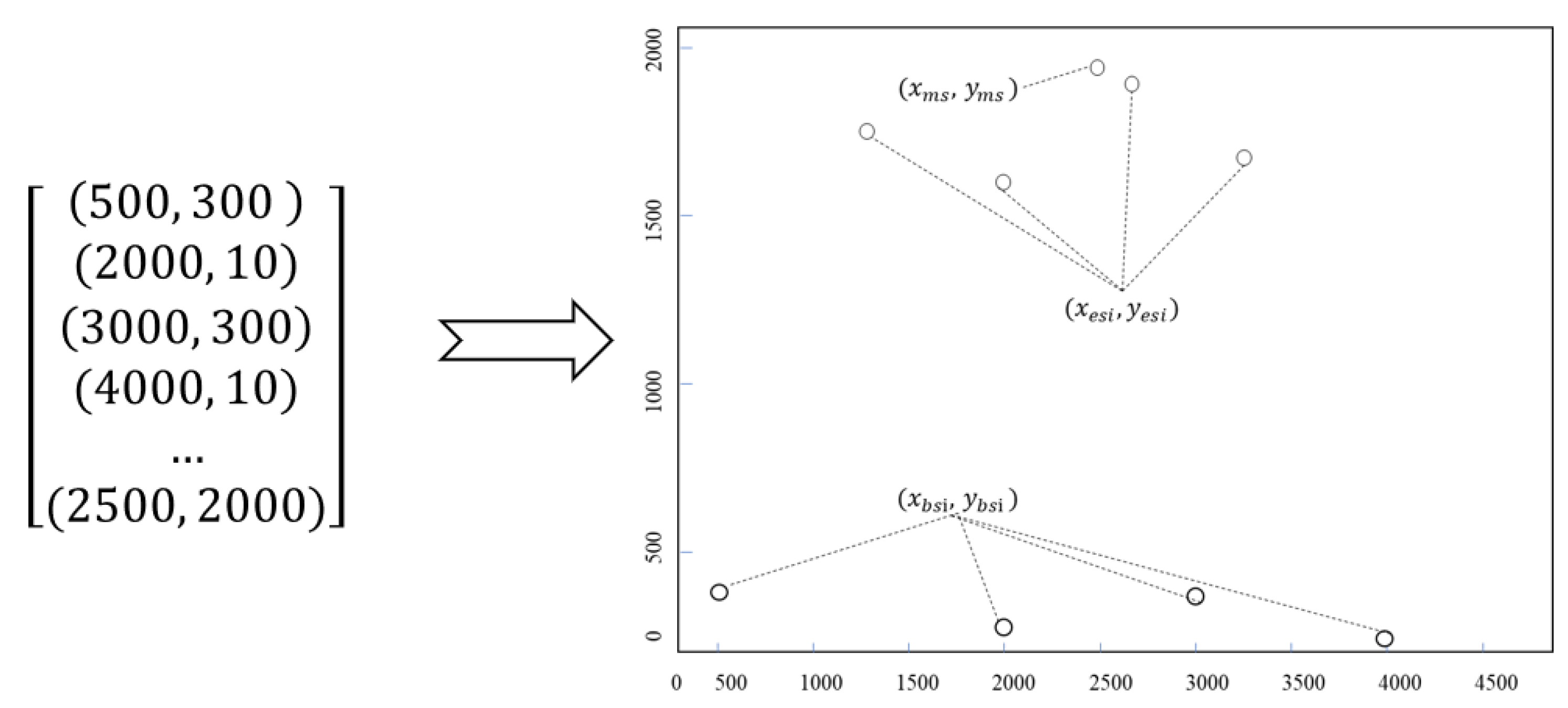
where $\left(x_{bsi},y_{bsi}\right)$ denotes the coordinates of the ith BS, $(x_{esi}$ and $y_{esi})$ denote the location coordinates of the ith group of BSs, and ${(x}_{ms},y_{ms})$ represents the target’s location.

Consider a scenario in which the location system has four BSs. Upon preliminary positioning, we obtain a 9 × 2 matrix containing four BS coordinates, four estimated coordinates, and a target location. The matrix is drawn into a coordinate image in a 2D coordinate system, where each coordinate point features the same size and color. Different node types and combinations are distinguished by the colors of the coordinate points. For example, the BS coordinates are black (RGB = (255, 255, 255)), whereas the actual MS coordinates are red (RGB = (255, 0, 0)). Finally, the coordinate matrix is transformed into a 64 × 64 pixel matrix, as shown in Figure 4.

4.4. Location Model of DenseNet

The main advantage of the DRSN is its ability to effectively process data that contain noise. DenseNet is a classic DRSN model that avoids the gradient vanishing problem caused by excessively deep network layers. This model accepts a 64 × 64 pixel matrix as an input and outputs the final estimated position of the target. In the online phase, a large amount of simulation data from different situations were used to train the models.

DenseNet was implemented to establish skip connections between the front and back layers in order to ensure that the layers of the whole neural network were deep enough to extract sufficient features. Because skip connections facilitate the reuse of information, denseness can achieve higher performance with fewer parameters and higher computational power. The neural network structure of DenseNet was designed as shown in Figure 5. DenseNet consists of two principal parts: a dense block and a transition.

In a dense block, all neural network layers have the same output size, and the input of each layer comes from the output of all previous layers. The dense block reuses information to ensure the completeness of the extracted data. The activation function of the dense block, which is represented by H, includes batch normalization, ReLU, and convolutional layers with a filter size of 3 × 3, which makes the extracted data more complete through information reuse. The output of layer i, $X_i$, is computed with Equation (8):

$$\begin{array}{c}{X}_i=H\left(\left[X_0,X_1,X_2,\dots X_{i-1}\right]\right)\end{array}$$

(8)

The transition layer of DenseNet can compress the model size by connecting two adjacent dense blocks. This layer contains a convolutional layer with a filter size of 1 × 1 and an AvgPooling layer with a filter size of 2 × 2. Assuming that its number of input channels is m, the transition layer can output $\lambda m$ channels, where the compression rate is $\lambda \in [0-1]$. When $\lambda =1$, the transition layer does not change the number of feature channels. When $\lambda$ is less than 1, this structure is called DenseNet-C, and it contains a dense block structure in the bottleneck layer and a transition with a compression coefficient that is less than 1.

5. Simulation Results

In this section, we evaluate the localization performance of the proposed NLOS error mitigation scheme. The effectiveness of the proposed location strategy was tested for different case studies within an operational scenario by using simulated data.The experimental environment included a software configuration and hardware configuration, as shown in

Table 1. Configuration information of the experimental environment.

Parameter	Value
CPU	Intel(R) Core(TM) i7-9750H
CPU Clock Speed	2.11 GHz
RAM	16 G
GPU	GeForce GTX 1660ti
Programming Language	Python 3.7
Software	Pycharm
Deep learning framework	PyTorch 1.7.0
CUDA Version	v10.2.89
CUDNN Version	v8.0.4

. The simulation was performed in MATLAB R2019b, and the process of radar ranging was conducted as follows. First, we generated an ideal parabolic pulse according to the set parameters and a Gaussian random noise signal according to the pulse width, pulse shape, and noise source. Next, we produced a noisy echo signal by superimposing an ideal echo signal with a random noise signal. We then obtained a smooth curve near the peak value by fitting the peak value of the filtered echo signal to a three-point parabola. Finally, the target distance value was calculated by using half of the corresponding peak time.

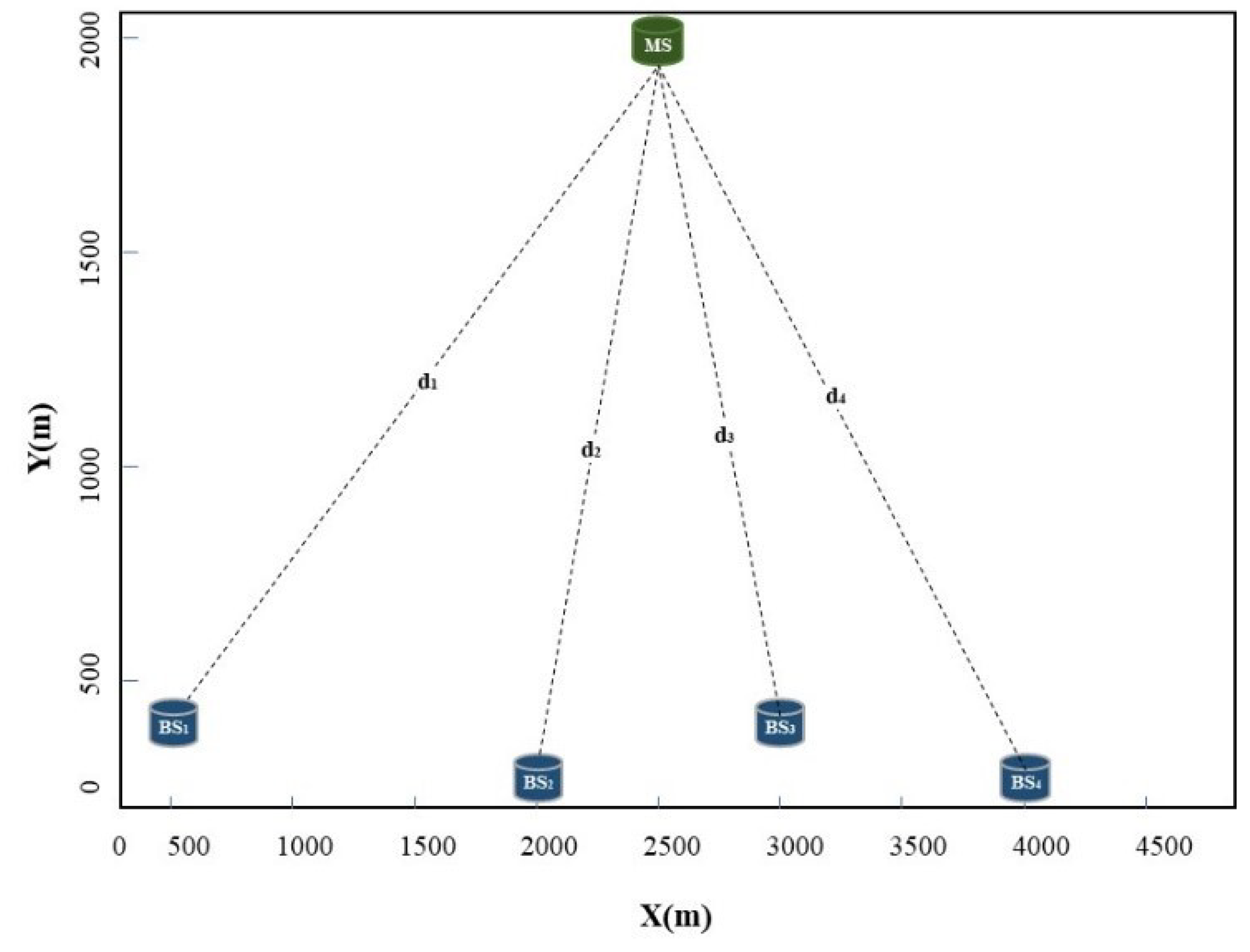
The simulation environment was equipped with four laser radars as BSs with coordinates at (500, 300), (2000, 10), (3000, 300), and (4000, 10). The target’s position was fixed at (2500, 2000). The NLOS error was drawn from a uniform distribution on the interval $[0.0d_i,0.9d_i]$, where $d_i$ expresses the measurement distance of the ith BS. The distributions of the BSs and targets are shown in Figure 6. Assuming that the number of BSs with a non-line-of-sight error is n$(0\le n\le 4)$, we independently executed 1000 simulations under different standard deviations $\sigma$ of Gaussian noise. For the proposed method, we generated 10,000 data as a training set and 2000 data as a test set. To assess the generality and eliminate the effect of the BS locations on the performance, we randomly selected BSs with NLOS propagation. The RMSE of the localization was used as a performance metric, and it was calculated using Equation (9):

$$RMSE=\sqrt{\frac{1}{N}\sum _{i=1}^N\left[{\left(x_i-\widehat{x_i}\right)}^2+{\left(y_i-\widehat{y_i}\right)}^2\right]}$$

(9)

where N is the number of test samples, and $(\widehat{x_i},\widehat{y_i},\widehat{z_i})$ and $(x_i,y_i,z_i)$ are the estimated and true coordinates, respectively, of the MS location of the ith test sample in meters.

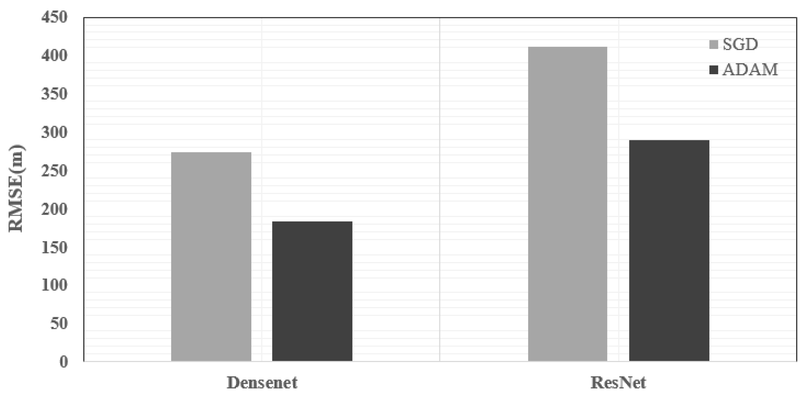
This experiment compared the performances of two classic DRSN models: DenseNet and ResNet. The solver was the algorithm that was used to train the deep learning model. Throughout the rigorous numerical verifications, it was observed that the DRSN models achieved better performance with the adaptive moment estimation (ADAM) optimizer. In Figure 7, it can be verified that the RMSE values for DenseNet and ResNet with the ADAM optimizer were lower than those with the stochastic gradient descent (SGD) optimizer. The training settings for the DenseNet model are presented in

Table 2. Training options for the DenseNet model.

Options	Value
Solver	Adam
Batch size	32
Epochs	250
Init. learning rate	0.0001

. In Figure 8, the number of NLOS links is shown, and the STD $\sigma$ is equal to 35 m. As shown in Figure 8, DenseNet yielded a lower loss and exhibited faster convergence in comparison with those of ResNet. This difference in performance can be attributed to the fact that DenseNet realized feature reuse through skip connections to avoid the problem of transmission of gradients between deep networks.

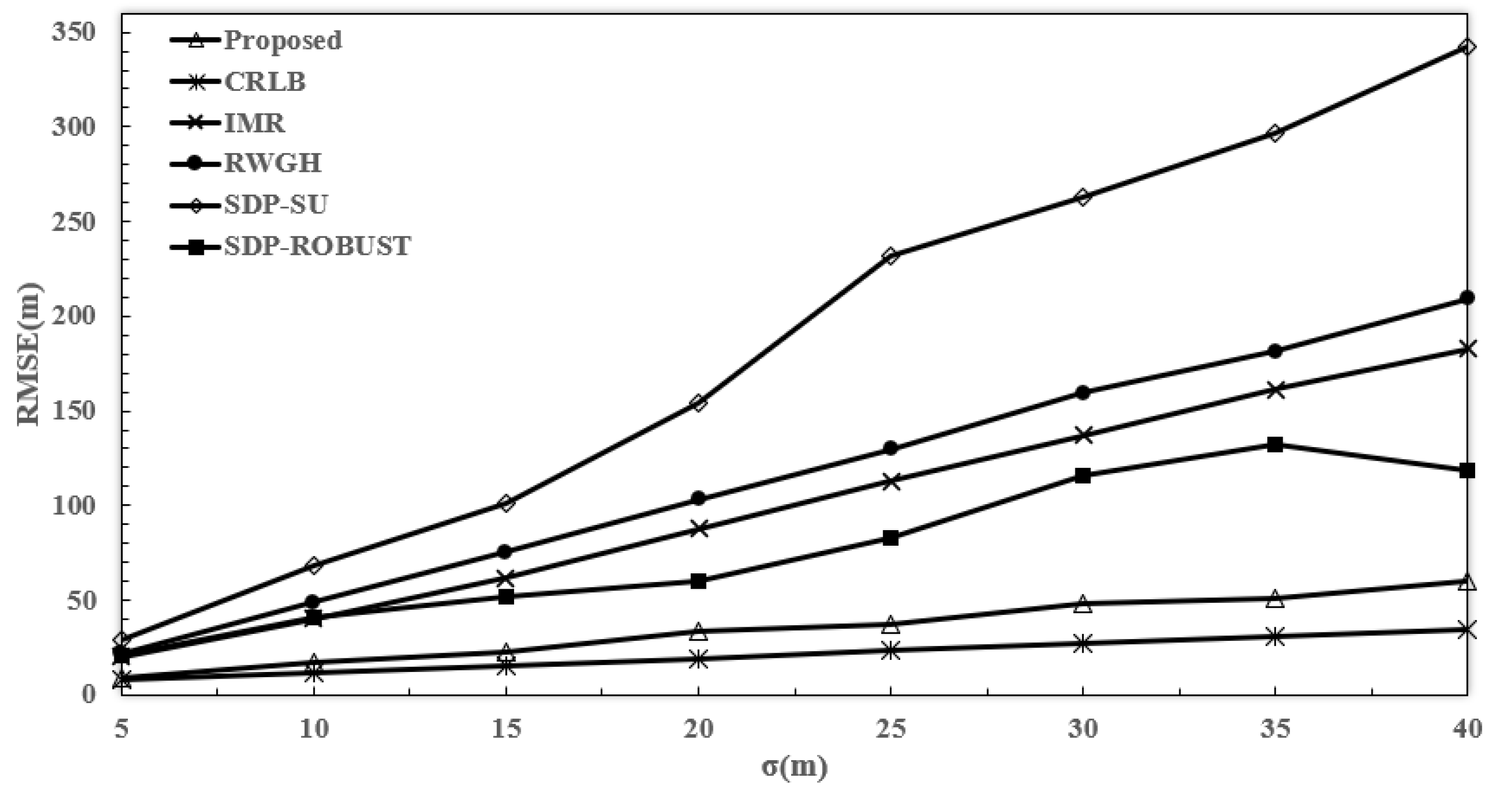
This experiment compared the RMSEs of the proposed model, RWGH [9], IMR [11], SR-ROBUST [12], and the model used by [13] (labeled as SDP-SU) across different values of $\sigma$. The Cramer–Rao lower bound (CRLB) was used as a reference to evaluate the algorithms’ performance. The simulation results of the RMSE versus $\sigma$ without NLOS BSs are shown in Figure 9. Here, as $\sigma$ increased from 5 to 40 m, the RMSE gradually increased for all methods. However, the proposed Pre-DenseNet algorithm exhibited the optimal performance. Our proposed algorithm came the closest to CRLB, and the RMSE was only 52.1 m for a standard noise deviation of 40 m.

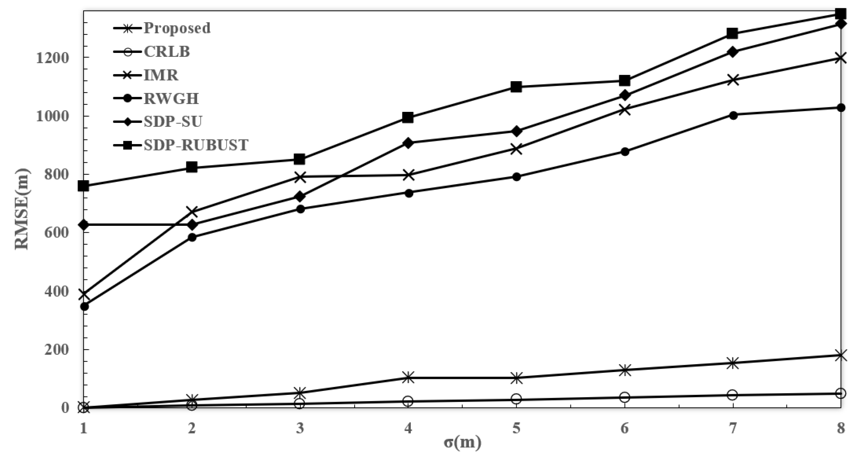
The simulation results of the measurement of the RMSE against $\sigma$ with one NLOS BS are shown in Figure 10. Here, it can be seen that the RMSEs of the other algorithms significantly increased with the LOS environment. However, with a $\sigma$ measurement error of 40, the RMSE of the proposed algorithm was only 156.23 m. In contrast, the minimum RMSE of the other two algorithms was 348.12 m, and the maximum RMSE was more than 1200 m.

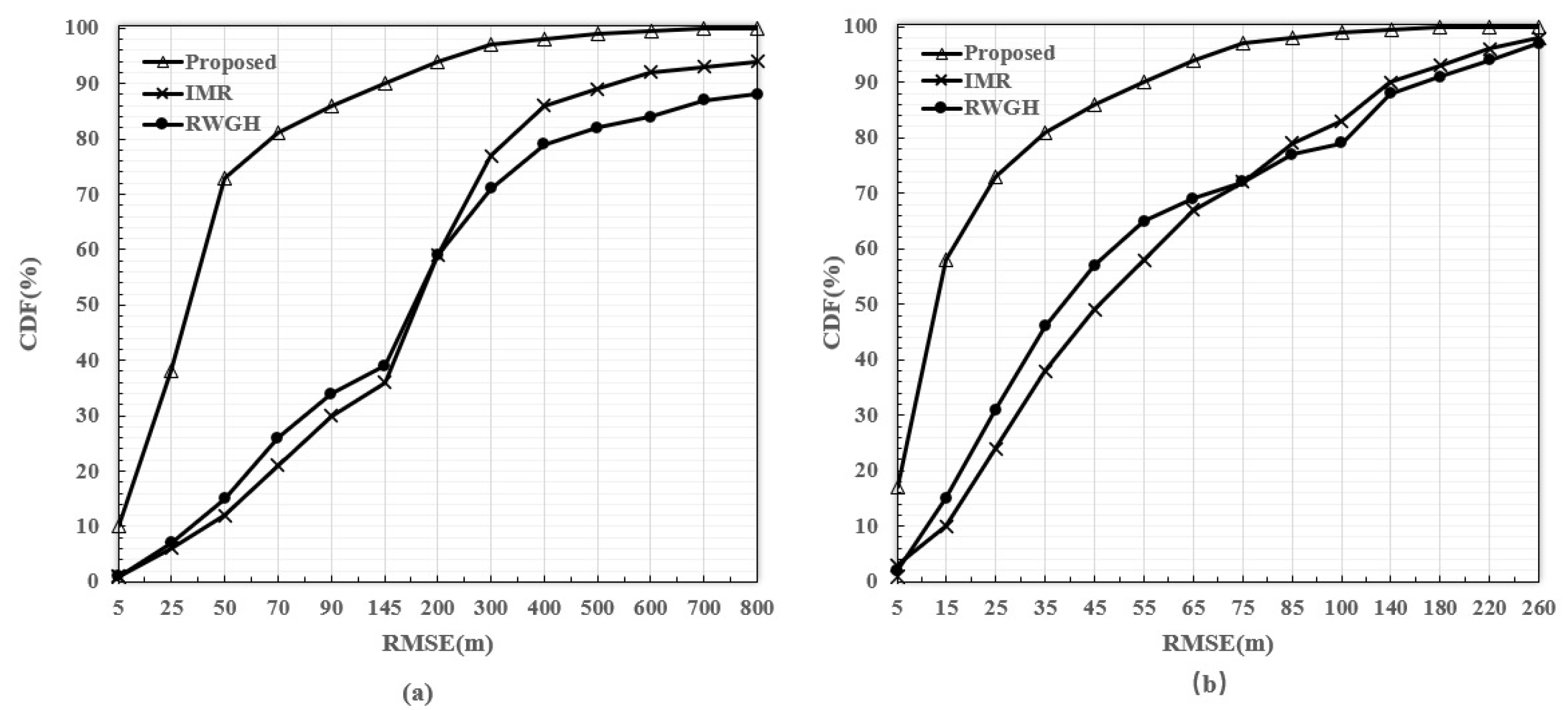
This experiment compared the corresponding cumulative distribution functions (CDFs) of the different algorithms when $\sigma$ was equal to 20 m. The results in Figure 11 illustrate the CDFs with and without an NLOS BS, which further verified the performance of the proposed algorithm in mixed NLOS and LOS environments. Here, the proposed DenseNet algorithm achieved optimal performance for the following reasons: (1) The data enhancement could fully excavate data features. The preliminary location grouping method allowed the DRSN model to identify the features of NLOS BSs. (2) The DRSN is a feature-learning method for strong noise and highly redundant data. DenseNet was adopted to establish skip connections between the front and back layers so that the layers of the whole neural network were deep enough to extract sufficient features.

For an analysis of the complexity of the different algorithms, the average computational time of each algorithm for N = 800 is shown in

Table 3. Training options for the DenseNet model.

Algorithm	Average Time
RWGH	1.16 s
IMR	0.62 s
SDP-SU	1.57 s
SDP-Robust	1.61 s
Proposed algorithm	2.19 s

. The proposed algorithm had the highest computational complexity because it needed data augmentation, which is a time-consuming process, especially for large environments. Since the proposed algorithm had a higher accuracy than that of the existing algorithms, it is the most attractive for practical applications.

6. Conclusions

In this paper, we proposed an effective method for identifying ships with abnormal AIS signals by comparing the positions and AIS tracks. The key problems with this technique are the influence of NLOS errors and the improvement of the positioning accuracy in special GDOP scenarios with fewer BSs. To address these issues, this paper proposes an efficient NLOS error mitigation scheme based on data enhancement and a DRSN. The input and output of the model are the radar-ranging information and the coordinates of the ship’s position, respectively. The simulation results demonstrated that the proposed method outperformed other range-based localization algorithms in a mixed LOS/NLOS environment. In the future, we intend to apply the proposed method to multi-device-fusion ranging scenarios, such as in the fusion radar ranging and visual ranging, because binocular stereo-vision ranging technology is easy to arrange and is more competitive than radar. There are also various interesting research topics, such as the time synchronization of radar ranging and visual ranging and the optimization of the anti-interference characteristics of visual ranging.

References

1. Joseph, A.; Dalaklis, D. The international convention for the safety of life at sea: Highlighting interrelations of measures towards effective risk mitigation. J. Int. Marit. Saf. Environ. Aff. Shipp. 2021, 5, 1–11. [Google Scholar] [CrossRef]
2. Katsilieris, F.; Braca, P.; Coraluppi, S. Detection of malicious AIS position spoofing by exploiting radar information. In Proceedings of the 16th International Conference on Information Fusion, Istanbul, Turkey, 9–12 July 2013; pp. 1196–1203. [Google Scholar]
3. Yu, K.; Guo, Y.J. Improved positioning algorithms for nonline-of-sight environments. IEEE Trans. Veh. Technol. 2008, 57, 2342–2353. [Google Scholar]
4. Guvenc, I.; Chong, C.C. A survey on TOA based wireless localization and NLOS mitigation techniques. IEEE Commun. Surv. Tutor. 2009, 11, 107–124. [Google Scholar] [CrossRef]
5. Qiao, T.; Liu, H. Improved least median of squares localization for non-line-of-sight mitigation. IEEE Commun. Lett. 2014, 18, 1451–1454. [Google Scholar] [CrossRef]
6. Gazzah, L.; Najjar, L.; Besbes, H. Improved hybrid AML algorithm without identification of LOS/NLOS Nodes. In Proceedings of the 2015 IEEE 81st Vehicular Technology Conference (VTC Spring), Glasgow, UK, 11–14 May 2015; pp. 1–5. [Google Scholar]
7. Zheng, X.; Hua, J.; Zheng, Z.; Zhou, S.; Jiang, B. LLOP localization algorithm with optimal scaling in NLOS wireless propagations. In Proceedings of the 2013 IEEE 4th International Conference on Electronics Information and Emergency Communication, Beijing, China, 15–17 November 2013; pp. 45–48. [Google Scholar]
8. Yang, K.; An, J.; Bu, X.; Lu, Y. A TOA-based location algorithm for NLOS environments using quadratic programming. In Proceedings of the 2010 IEEE Wireless Communication and Networking Conference, Sydney, NSW, Australia, 18–21 April 2010; pp. 1–5. [Google Scholar]
9. Chen, P.C. A non-line-of-sight error mitigation algorithm in location estimation. In Proceedings of the WCNC. 1999 IEEE Wireless Communications and Networking Conference (Cat. No. 99TH8466), New Orleans, LA, USA, 21–24 September 1999; Volume 1, pp. 316–320. [Google Scholar]
10. Wu, S.; Xu, D.; Wang, H. Adaptive NLOS mitigation location algorithm in wireless cellular network. Wirel. Pers. Commun. 2015, 84, 3143–3156. [Google Scholar] [CrossRef]
11. Li, X. An iterative NLOS mitigation algorithm for location estimation in sensor networks. In Proceedings of the 15 th IST Mobile and Wireless Communications Summit, Mykonos, Greece, 4–8 June 2006; pp. 1–5. [Google Scholar]
12. Wang, G.; So, A.M.C.; Li, Y. Robust convex approximation methods for TDOA-based localization under NLOS conditions. IEEE Trans. Signal Process. 2016, 64, 3281–3296. [Google Scholar] [CrossRef]
13. Su, Z.; Shao, G.; Liu, H. Semidefinite programming for NLOS error mitigation in TDOA localization. IEEE Commun. Lett. 2017, 22, 1430–1433. [Google Scholar] [CrossRef]
14. Tomic, S.; Beko, M. A bisection-based approach for exact target localization in NLOS environments. Signal Process. 2018, 143, 328–335. [Google Scholar] [CrossRef] [Green Version]
15. Falsi, C.; Dardari, D.; Mucchi, L.; Win, M.Z. Time of arrival estimation for UWB localizers in realistic environments. EURASIP J. Adv. Signal Process. 2006, 2006, 1–13. [Google Scholar] [CrossRef] [Green Version]
16. Marano, S.; Gifford, W.M.; Wymeersch, H.; Win, M.Z. NLOS identification and mitigation for localization based on UWB experimental data. IEEE J. Sel. Areas Commun. 2010, 28, 1026–1035. [Google Scholar] [CrossRef] [Green Version]
17. Mucchi, L.; Marcocci, P. A new parameter for UWB indoor channel profile identification. IEEE Trans. Wirel. Commun. 2009, 8, 1597–1602. [Google Scholar] [CrossRef]
18. Momtaz, A.A.; Behnia, F.; Amiri, R.; Marvasti, F. NLOS identification in range-based source localization: Statistical approach. IEEE Sensors J. 2018, 18, 3745–3751. [Google Scholar] [CrossRef]
19. Go, S.; Chong, J.W. An efficient TOA-based localization scheme based on BS selection in wireless sensor networks. IEICE Trans. Commun. 2014, 97, 2560–2569. [Google Scholar] [CrossRef]
20. Wang, Y.; Jing, Y.; Jia, Z. An indoor mobile localization strategy for robot in NLOS environment. Int. J. Distrib. Sens. Netw. 2013, 9, 758749. [Google Scholar] [CrossRef]
21. Yu, K.; Guo, Y.J. Statistical NLOS identification based on AOA, TOA, and signal strength. IEEE Trans. Veh. Technol. 2008, 58, 274–286. [Google Scholar] [CrossRef]
22. Sharp, I.; Yu, K.; Guo, Y.J. GDOP analysis for positioning system design. IEEE Trans. Veh. Technol. 2009, 58, 3371–3382. [Google Scholar] [CrossRef]
23. Muqaibel, A.H.; Al-Nimnim, R.A.; Landolsi, M.A.; Al-Ahmari, A.S. Mobile localization based on improved non-line-of-sight classification. In Proceedings of the 2010 17th International Conference on Telecommunications, Doha, Qatar, 4–7 April 2010; pp. 368–374. [Google Scholar] [CrossRef]
Figure 1. The location model in cellular networks.
Jmse 10 01952 g001
Figure 2. The location model for coastal scenarios.
Jmse 10 01952 g002
Figure 3. The influence of GDOP on location. (a) Two NLOS BSs in the same direction. (b) Two NLOS BSs in the opposite direction.
Jmse 10 01952 g003
Figure 4. Spatial coordinate relationship model with one MS and four BSs. Different node types and combinations have the same size and different colors.
Jmse 10 01952 g004
Figure 5. The structure of DenseNet with three dense blocks and two transitions.
Jmse 10 01952 g005
Figure 6. The layout of the BSs and the target.
Jmse 10 01952 g006
Figure 7. RMSEs of the DenseNet and ResNet models with the SGD and ADAM optimizers.
Jmse 10 01952 g007
Figure 8. RMSE performance with the training data for DenseNet and ResNet.
Jmse 10 01952 g008
Figure 9. RMSE performance (Y-axis) across different standard deviations of the measurement error (X-axis: σ ) without NLOS BSs.
Jmse 10 01952 g009
Figure 10. RMSE performance (Y-axis) across different standard deviations of the measurement error (X-axis: σ ) with one NLOS BS.
Jmse 10 01952 g010
Figure 11. CDFs of the RMSE with σ = 20 m. (a) The CDF with one NLOS BS. (b) The CDF without NLOS BSs.
Jmse 10 01952 g011