Abstract
As one of the ship energy efficiency optimization measures with the most energy saving and emission reduction potential, ship speed optimization has been recommended by the International Maritime Organization. In ship speed optimization, considering the influence of weather conditions, route segmentation and weather data loading methods significantly affect the reliability of speed optimization results. Therefore, taking the ocean-going container ship as the research object, on the basis of constructing the main engine fuel consumption prediction model and shaft speed prediction model based on machine learning methods, a route segmentation and weather loading-speed optimization iterative algorithm is proposed in this study. Single-objective speed optimization research is then conducted based on the algorithm. The research results show that the proposed algorithm effectively reduces the difference between optimized fuel consumption and actual fuel consumption, and can achieve a fuel-saving rate between 2.1% and 5.2%. This study achieves an accurate and reliable prediction of ship fuel consumption and shaft speed, and solves the strong coupling problem between route segmentation, weather loading, and speed optimization by iterative optimization of ship speed. The proposed algorithm provides strong technical support for ships to achieve the goal of energy saving and emission reduction.
1. Introduction
The impact of the shipping industry on the environment is increasing day by day, with the issue of greenhouse gas emissions generated by the shipping industry attracting extensive attention from the international community. In June 2021, the 76th session of the Marine Environment Protection Committee of the International Maritime Organization (IMO) formally adopted amendments to the International Convention for the Prevention of Pollution from Ships (MARPOL) Annex VI. These amendments introduced mandatory technical and operational approaches to reduce the carbon intensity of international shipping, requiring all ships to meet not only the Energy Efficiency Existing Ship Index (EEXI) requirements, but also annual operational carbon intensity indicator (CII) requirements after the rules come into force. At the same time, ship operators are also required to rate ships from A to E according to their annual operational energy efficiency. For ships rated below C, they may face a series of problems in their subsequent operations [1].
In an international environment with increasingly stringent requirements for reducing greenhouse gas emissions, shipping companies are eager to find a ship energy efficiency optimization measure to optimize ship operations, in order to reduce ship fuel consumption, greenhouse gas emissions, and operating costs. In 2018, the initial strategy for reducing greenhouse gas emissions from ships adopted by the IMO indicated that possible short-term emission reduction measures include improving the existing ship energy efficiency framework, optimizing or reducing ship speed, and developing alternative low-carbon or zero-carbon fuels, etc. [2]. Among them, ship speed optimization is one of the most effective and convenient ship operation optimization measures for existing ships to achieve energy saving and emission reduction, and can significantly reduce ship fuel consumption, emissions, and costs. Nevertheless, there are still some problems in the current research on ship speed optimization, such as the method of route segmentation based on the weather is not mature enough, and there is a large gap between the optimized fuel consumption and the actual fuel consumption.
The route segmentation and the weather data loading on the segment are the basis for ship speed optimization, so the route must be segmented and the weather on the segment must be obtained before speed optimization. At present, the route segmentation methods in the field of speed optimization can be roughly divided into two types: one is segmenting by one day, half a day, etc., according to the length of the sailing time [3,4]; the other is segmenting by cluster analysis based on the weather data on the route [5,6,7]. These two types of methods usually need to ensure that the ship’s course is the same at each waypoint within the segment, so the first type of method can be called the turning point-time segmentation method and the second type of method can be called the turning point-clustering segmentation method. At the same time, only one type of weather can be used for each segment and, thus, as the weather for the whole segment, the weather data within the segment are usually averaged.
From the perspective of sailing time, the turning point-time segmentation method takes relatively little consideration of the weather data on the route, which may cause the problem of large differences in weather at each point within a segment. However, this problem can be improved by shortening the sailing time used for route segmentation. The turning point-clustering segmentation method performs cluster analysis based on the weather data on the route to ensure that the weather at each point within the segment is as similar as possible, thus enabling weather-based route segmentation. Nevertheless, in speed optimization, the clustering methods used for route segmentation are usually unordered methods such as k-means [5,6,7], which do not consider the ordered attributes of each point on the route, making it difficult to control the quality and quantity of segmentation and increasing the uncertainty of route segmentation. Therefore, there is still some room for improvement and research on the methods related to ship speed optimization, with relevant research needed to promote the continuous development and maturity of ship speed optimization methods and strategies.
The rest of the paper is organized as follows. Section 2 reviews the relevant literature and clarifies the research gaps. Section 3 introduces the modeling method of fuel consumption and shaft speed, as well as the route segmentation-weather loading-speed optimization method. Section 4 describes the optimization objective and constraints. Section 5 conducts the case study and results discussion. Finally, conclusions are drawn in Section 6.
2. Literature Review and Research Gaps
2.1. Literature Review
In recent years, to achieve the goal of ship energy saving and emission reduction, a large number of scholars and practitioners in the shipping industry have conducted fruitful research on ship speed optimization [8,9,10,11,12,13]. In these studies, ship speed optimization considering the influence of weather conditions is one of the focuses of researchers. Noting that the fuel consumption of inland ships is affected by wind speed, wind direction, water speed, and water depth, Wang et al. [14] proposed a new dynamic (rolling) optimization method adopting the model predictive control strategy to optimize ship speed. Their method considers the influence of time-varying environmental factors, which is a progress in the field of speed optimization for inland ships. However, they segment the route only based on the time step, so their segmentation method is relatively simple. For ocean-going ships, Yang et al. [15] developed a speed optimization model considering the influence of ocean currents for a fixed route. Their experimental results show that the developed model can effectively reduce the error between estimated speed over ground (SOG) and measured SOG, thereby significantly reducing the fuel consumption and emissions of ships. Considering the time span and accuracy of the currently available weather forecast services, Tzortzis and Sakalis [16] proposed a method to dynamically determine the optimal ship speed on a fixed route. They address the problem of the decreased accuracy of weather forecasts for longer time periods by dividing the total time horizon of the route into smaller time periods. Their application on an actual container ship route verifies the effectiveness of the method. In addition, similar studies include Li et al. [17], which considers voluntary and involuntary speed loss, and Hu [11], which considers weather conditions for route selection and speed optimization. Nevertheless, these studies still seldom discuss route segmentation and weather data loading methods in depth in ship speed optimization.
Therefore, some studies focus on the problem of route segmentation based on weather conditions. Wang et al. [7] used the k-means clustering algorithm to cluster and analyze the historical data of wind speed, wind direction, water speed, and water depth on the inland river route, and then divided the route into 97 segments. Based on MapReduce’s distributed parallel k-means clustering algorithm, Yan et al. [6] realized the segmentation of inland river routes in the dry and rainy seasons, and then used the particle swarm algorithm to solve the optimal engine speed on each segment. Similarly, Wang et al. [5] first performed cluster analysis on the historical data of wind speed, wind direction, wave height, current speed, and current direction on the ocean route based on the k-means clustering algorithm to establish a knowledge base of sea state categories. On this basis, they realized the identification of sea state and route segmentation through the k-nearest neighbor classification algorithm, and finally completed the dynamic optimization of ship speed by using the genetic algorithm. The above studies preliminarily explored the route segmentation problem in ship speed optimization. However, due to the unordered clustering property of the k-means clustering algorithm that they adopted, the same type of segment is distributed in different positions of the route, and the number of segments is large and uncontrollable, which will eventually cause frequent adjustment of ship speed.
In addition, the development of machine learning methods is further advancing research in the field of ship speed optimization [18,19]. Lee et al. [20] used weather archive data to estimate the actual fuel consumption of ships in a speed optimization problem. They used the Copernicus dataset as a source of big data and applied data mining techniques to identify the impact of weather conditions on fuel consumption based on a given route. To quantify the synergistic effects of speed, displacement, trim, weather, and sea state on ship fuel consumption, Du et al. [3] first developed artificial neural network (ANN) fuel consumption prediction models based on voyage report data from two 9000-TEU container ships, and then conducted joint speed-trim optimization. They focused on the daily speed planning of ships and verified it with voyage report data. Finally, they reported that joint speed-trim optimization can achieve a fuel-saving rate of more than 4.96%. Zheng et al. [21] constructed an ANN model to predict cruise ship fuel consumption based on automatic identification system (AIS) data. Meanwhile, they used four improved particle swarm algorithms to optimize ship speed after dividing the route into 12 segments based on sailing stations. Their results show that the multi-swarm cooperative particle swarm optimization algorithm can achieve better optimization results. However, their method of dividing segments according to stations is relatively simple, and there is still some room for improvement. Based on the voyage report data of a dry bulk carrier and the random forest (RF) method, Yan et al. [4] constructed a fuel consumption prediction model for ship speed optimization. It is noteworthy that they applied a data smoothing algorithm to smooth the fuel consumption–ship speed trend predicted by the model considering the breakpoint problem of the RF model. On this basis, the comparison results with the daily voyage report data show that their optimization model can achieve a fuel-saving rate between 2% and 7%. Due to the better fuel-saving effect, the research on ship speed optimization based on the machine learning method gradually shows its advantages, but there is still some room for development in route segmentation and weather data loading.
2.2. Research Gaps
Ship speed optimization is usually performed for unsailed voyages, while the actual weather encountered by the ship during future voyages is closely related to the speed, i.e., the dynamic correlation between weather and time-position (speed). Therefore, before sailing, it is usually difficult to accurately determine the actual weather conditions encountered on the route in the future, which reveals the strong coupling among route segmentation, segment weather loading, and speed optimization. Through the literature review, it is not difficult to find the following research gaps in the existing literature:
- (1)
- At present, the research on ship speed optimization considering the actual weather influence on fixed routes between two ports is still immature, and the research on route segmentation and weather loading methods based on real-time weather has just started. Some studies segment the route only according to time steps [14,16], or segment after unordered clustering based on the ship’s historical navigation data [6,7], which leads to a large number of segments or difficulty controlling the number of segments. In addition, the dynamic correlation between real-time weather and ship speed is also less considered.
- (2)
- Some studies conduct ship daily speed optimization and verification based on ship navigation report data [3,4], but there are relatively few explorations on route segmentation and weather loading before sailing. Therefore, these studies usually validate the algorithms under the assumption that the route segmentation is known (the route is segmented by turning point (station) or by sailing time (one day) based on voyage reports), and that the weather conditions for each segment are known and fixed. On the one hand, segmentation of the route by turning point or time may result in large weather differences within each segment; on the other hand, before the ship sails, the daily distance the ship travels and the weather of each segment are usually unknown. Therefore, these problems cause some limitations and room for improvement in the practical application of this kind of research.
- (3)
- The existing studies usually solve the speed optimization problem only once [17,22], which will result in a gap between the theoretical calculation and the practical application, i.e., there is a difference between the optimized fuel consumption based on a specific set of weather and sea condition data in the theoretical calculation and the actual (simulated) fuel consumption obtained by the ship sailing at optimized speed. This is due to the change in weather and sea conditions encountered while the ship is sailing at the optimized speed compared to the beginning of the optimization.
2.3. Research Contributions
To bridge the research gap in the speed optimization literature in terms of the rationality of route segmentation, the dynamics of weather loading, and the accuracy of optimized fuel consumption, and to make the speed optimization results more practical, we propose a route segmentation-weather loading-speed optimization iterative algorithms considering the actual weather. We will report the related research on the weather loading-speed optimization iterative algorithm based on an improved turning point-time segmentation method in this paper. This study provides industry professionals with practical solutions for ship speed optimization and intensive experimental evidence from different case routes.
The contribution of this study to the field of ship speed optimization can be summarized in the following two aspects:
- (1)
- This study constructs an accurate and reliable ship main engine fuel consumption prediction model and shaft speed prediction model based on machine learning methods and model fusion ideas, thus realizing an effective trade-off between the accuracy and reliability of fuel consumption and shaft speed prediction in ship speed optimization. The constructed shaft speed prediction model solves the matching problem between the optimal ship speed and the optimal shaft speed in ship speed optimization and improves the practicality of the speed optimization results. The modeling method of this study provides a new way to obtain accurate and reliable ship fuel consumption and shaft speed in ship speed optimization.
- (2)
- This study proposes an iterative algorithm for route segmentation and weather loading-speed optimization, which solves the strong coupling problem between route segmentation, weather loading, and speed optimization. The proposed algorithm ensures the rationality of route segmentation, realizes the dynamic loading of weather data, and reduces the error between optimized fuel consumption and actual fuel consumption, thus reducing the gap between the theoretical research of speed optimization and the practical application of shipping companies. The optimization method of this study significantly improves the reliability and practicality of speed optimization in actual ship operation, achieves significant fuel-saving effects, and can provide effective technical means for shipping companies to achieve the goal of energy saving and emission reduction.
3. Model and Method
3.1. Prediction Models of Ship Main Engine Fuel Consumption and Shaft Speed
The prediction accuracy of ship main engine fuel consumption is related to the effectiveness of ship speed optimization results. Therefore, to accurately predict the ship main engine fuel consumption under the influence of weather, this paper adopts the machine learning method to construct a ship main engine fuel consumption prediction model. The data used for modeling come from the sensor data collected by a container ship (the main information is shown in Table 1) from May to November 2015, and the collection interval is 15 min. After the data pre-processing program, 11,821 data remain in the sensor dataset, with the distribution of speed over ground (SOG) and daily fuel consumption of the main engine shown in Figure 1.

Table 1.
Ship information.
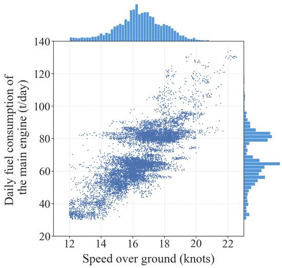
Figure 1.
Distribution of SOG and daily fuel consumption of the main engine.
Considering the application scenarios of the model, the selected model input features are SOG, trim, mean draft, wind speed, wind direction, wave direction, significant height of combined wind waves and swell (wave height), wave period, seawater temperature, current speed, and current direction, and the model output feature is the daily fuel consumption of the main engine. Since the sensor dataset does not contain wave, current, and seawater temperature data, the data fusion method proposed by Du et al. [23] is used to supplement the wave and seawater temperature data from the European Centre for Medium-Range Weather Forecasts (ECMWF) [24,25] (data granularity of 0.25° (longitude × 0.25° (latitude) × 6 (time)) and current data from the Copernicus Marine Service (CMEMS) [26] (data granularity of 0.25° (longitude) × 0.25° (latitude) × 3 (time)). All direction data in the modeling dataset are converted into the angle between the direction of the feature and the vector from the bow to the stern, ranging from 0° (head wind/wave/current) to 180° (following wind/wave/current). In addition, when modeling, the dataset is divided into a training set and a test set containing 80% and 20% of the data volume, respectively.
When choosing a machine learning method for modeling, we consider the following three aspects:
- (1)
- Li et al. [27] and Du et al. [23] suggest that the extremely randomized trees (ET) method [28], based on the principle of decision tree ensemble, has the highest prediction accuracy. The strategy used by the ET method to integrate decision trees is the bagging ensemble strategy, which essentially improves the model fitting performance by reducing the variance of the model. The ET method can reduce prediction errors and variance, and effectively prevent overfitting by combining different decision trees. Moreover, the comparison experiments on the prediction accuracy of multiple machine learning methods conducted on the modeling dataset of this study also confirm that the ET method has the highest fuel consumption prediction accuracy (see Appendix A for the specific comparison results). Therefore, the ET method is chosen as one of the methods to construct the fuel consumption prediction model in this study.
- (2)
- The results of Yan et al. [4] indicate that there is a breakpoint phenomenon in the variation trend of ship fuel consumption with speed predicted by the decision tree ensemble model. Therefore, it is necessary to find a suitable way to solve this problem.
- (3)
- The third-order polynomial regression (PR) method can better reflect the approximate cubic relationship between ship speed and main engine fuel consumption, and the predicted variation trend of ship fuel consumption with speed is relatively smooth and reliable.
Therefore, to balance the accuracy and reliability, this study uses the voting regressor in the scikit-learn library [29] to construct a VR integrated model based on the ET and PR model for the prediction of fuel consumption in ship speed optimization, with the Hyperopt library [30] used to optimize the model hyperparameters when building the ET model (see Appendix A and Li et al. [27] for the specific method). The idea behind the voting regressor is to combine conceptually different machine learning regressors and return the average predicted values. Such a regressor can be useful for a set of equally well performing models in order to balance out their individual weaknesses [29]. Table 2 and Figure 2 show the accuracy differences on the test set and the trend reliability differences on some test segments before and after model integration, respectively, where the accuracy evaluation metrics are R2, root mean square error (RMSE), mean absolute error (MAE), and mean absolute percentage error (MAPE).
Table 2.
Accuracy differences before and after fuel consumption model integration on the test set.
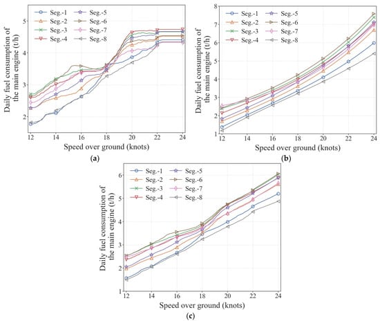
Figure 2.
Trend reliability differences before and after fuel consumption model integration on test segments. (a) ET model. (b) PR model. (c) VR model.
It can be seen from Table 2 that the prediction accuracy of the VR model is slightly weaker than that of the ET model but significantly stronger than that of the PR model, indicating that the VR model still has relatively high prediction accuracy. In terms of prediction reliability, it can be seen from Figure 2 that the VR model has a more reasonable and smooth speed-main engine fuel consumption variation trend than the ET model, and there is no obvious breakpoint phenomenon. The VR model combines the high accuracy advantages of the ET model and the strong reliability advantages of the PR model, laying a solid and reliable model foundation for the subsequent ship speed optimization.
In addition, in actual sailing, the ship usually changes the ship speed by directly adjusting the speed of the main engine (shaft). Therefore, to obtain the optimal shaft speed corresponding to the optimal ship speed, the shaft speed prediction VR model is constructed in the same integrated way as the main engine fuel consumption prediction model, with the input features of the two models consistent. Moreover, considering the approximate linear relationship between the ship speed and the shaft speed, the highest order of the integrated PR model is set to the first order. The prediction accuracy and trend reliability of the shaft speed prediction model are shown in Table 3 and Figure 3, respectively, from which it can be seen that the established model has high accuracy and reasonable trend, which provides a guarantee for the subsequent accurate and reliable prediction of shaft speed.
Table 3.
The prediction accuracy of the shaft speed prediction model on the test set.
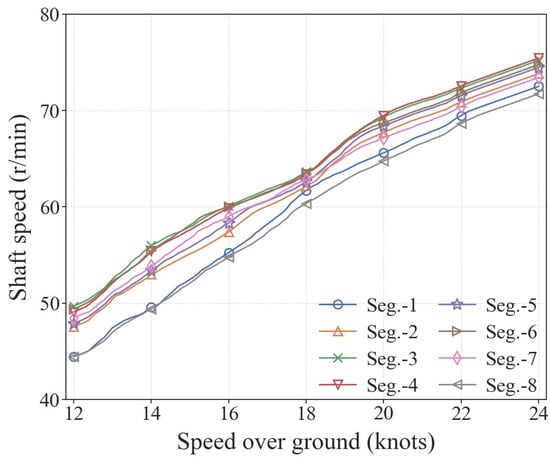
Figure 3.
The trend prediction reliability of the shaft speed prediction model on test segments.
3.2. Route Segmentation Method and Weather Loading-Speed Optimization Iterative Algorithm
The turning point-time segmentation method is simple in calculation and has a good engineering application effect. It is mostly used by shipping companies for daily ship speed planning. However, segmenting the route on a one-day basis may make the unique average weather of segments unrepresentative. Therefore, to solve the route segmentation problem, we improve the turning point-time segmentation method by shortening the sailing time used for route segmentation, and then propose an effective and practical route segmentation method. In addition, to avoid frequent changes in ship speed within a short period of time, the sailing time of the ship on each segment should not be too short, which requires a trade-off between the accuracy of route segmentation and the sailing time of the ship. To determine a suitable time benchmark for route segmentation and to match the actual ship navigation as much as possible, the SOG data of a certain day in the ship sensor dataset is visualized to analyze the speed change within a day, as shown in Figure 4.
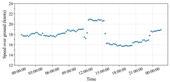
Figure 4.
Changes in SOG within a day.
From Figure 4, it can be seen that SOG has roughly four obvious changes in a day, and the relatively stable time periods for sailing speed are: 0:00 to 8:15, 8:45 to 11:30, 12:30 to 15:15, 15:45 to 20:15, and 20:45 to 23:15. By analyzing the SOG data, it can be seen that the shortest stable sailing time of the ship is about 3 h, the longest is about 9 h, and no more than 12 h. Therefore, to make the sailing time of the ship on each segment approximately range between 3 h and 12 h, a new turning point-time segmentation method is proposed, and specifically includes the following five steps:
(1) Based on the latitude and longitude data of the turning points given by the planned route, the ship course and distance between adjacent turning points are calculated according to the rhumb line formulas [31]:
where and are the longitudes of the starting and ending points, respectively; and are the latitudes of the starting and ending points, respectively; is the ship course between two adjacent turning points, deg; and is the distance between two adjacent turning points, n mile.
(2) The distance between adjacent turning points is accumulated to obtain the route distance, with the average ship speed on the route then calculated according to the route distance and the latest arrival time.
(3) The sailing time of the ship between adjacent turning points and the time to arrive at each turning point are estimated according to the average ship speed.
(4) Based on the formula for calculating the number of segments of the sub-route between adjacent turning points shown in Formula (6), the sub-route between adjacent turning points is divided into several segments equally by distance (the sub-route with a sailing time of less than 6 h is not segmented), so that the sailing time of the ship in each segment approximately ranges between 3 h and 12 h and the ship course at each point in any segment is guaranteed to be the same.
where is the number of segments of the sub-route between adjacent turning points; is the ceiling function; and is the ship sailing time between adjacent turning points, h.
(5) Based on the distance of each segment and the longitude and latitude of the turning points, the rhumb line formulas [31] are used to calculate the longitude and latitude coordinates of each segmentation point. At the same time, the time for the ship to arrive at each segmentation point is calculated according to the distance of each segment and the average ship speed, in order to obtain the final route segmentation data.
After completing the route segmentation, it is necessary to load the corresponding weather data on each segment as the input of the speed optimization model. The weather data on the route are related to the geographical location and time, but the time when the ship arrives at a specific position on the route is unknown before the ship speed optimization is performed. Therefore, to solve this contradictory relationship, an iterative algorithm for route weather loading-speed optimization is proposed, with the algorithm flow chart shown in Figure 5.
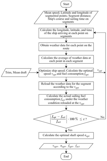
Figure 5.
Flow chart of weather loading-speed optimization iterative algorithm.
Figure 5 clearly shows the overall framework of the route weather loading-speed optimization iterative algorithm based on the turning point-time segmentation method, whose principle is to reduce the fuel consumption error to a small reasonable range through multiple weather loading iterations and speed optimization iterations. By using this algorithm, the matching degree between the route weather and the optimal speed can be gradually improved, and the gap between the optimal fuel consumption and the actual fuel consumption can be reduced. In addition, the waypoints used to obtain the weather data on segments in this algorithm are the position points reached by the ship every 15 min, which is consistent with the sensor data collection interval.
4. Objective and Constraints of Ship Speed Optimization
The ship speed optimization considering the weather conditions aims to optimize the ship speed on each segment according to the weather conditions on each segment to minimize the fuel consumption of the main engine on the whole route. Therefore, based on the establishment of an accurate and reliable main engine fuel consumption prediction model, the speed optimization objective with the lowest fuel consumption of the main engine for a single voyage is constructed, with the specific objective function as follows:
where is the total fuel consumption of the main engine of the ship on the route, t; is the number of segments of the route; is the fuel consumption of the main engine on the segment , t/h; is the distance of segment , n mile; is the SOG of the ship on segment , knots; is the main engine fuel consumption VR model; is the mean draft of the ship on the segment , m; is the trim of the ship on the segment , m; is the wind speed on segment , knots; is the wind direction on the segment , °; is the wave height on the segment , m; is the wave direction on the segment , °; is the wave period on the segment , s; is the current speed on segment , knots; is the current direction on the segment , °; and is the seawater temperature on the segment , ℃.
To ensure that the ship arrives at the destination port on time and operates normally and safely, the speed optimization problem should include the latest arrival time constraint (Formula (9)), the maximum speed constraint (Formula (10)), the minimum speed constraint (Formula (11)), and the critical speed constraint (Formula (12)). In these constraints, the critical speed of the ship is estimated according to the voluntary speed loss Formula (13) [17] under different sea conditions to ensure the safety of ship navigation as much as possible.
where is the latest arrival time, h; is the maximum speed of the ship in normal sailing, knots; is the minimum speed of the ship in normal sailing, knots; is the critical speed of the ship on segment , knots; is the design speed of the ship, knots; and and are two coefficients related to the wind direction and Beaufort scale on each segment, respectively [32].
The main engine fuel consumption model in the objective function of speed optimization is a data-driven model constructed based on machine learning methods, so it is highly nonlinear. On the one hand, nonlinear algorithms such as the interior point method are difficult to solve this optimization problem effectively; on the other hand, although heuristic algorithms such as the genetic algorithm can solve this optimization problem in a certain time, the optimization results obtained are feasible solutions rather than optimal solutions, and there are fluctuations in the optimization results. Therefore, these algorithms are relatively difficult to use for solving the speed optimization problem in this study.
Considering that the maximum adjustment accuracy of the speed in the actual navigation of the ship is 0.1 knots, the too-precise continuous solution of the optimized speed is meaningless in practical applications. Therefore, the idea of discrete optimization can be introduced to transform the nonlinear continuous optimization problem of speed optimization into a linear discrete optimization problem; thus, this speed optimization problem can be solved effectively. The specific variable discretization method is to discretize the speed from the minimum speed to the maximum speed at an interval of 0.1 knots: , and introduce the auxiliary decision variable to transform the nonlinear optimization problem into a 0–1 mixed integer linear programming problem. In this programming problem, each discrete speed on each segment corresponds to an auxiliary decision variable, and it is stipulated that only one auxiliary decision variable has a value of 1 on the same segment, while the rest are 0. After transformation, the objective function and constraints of ship speed optimization are:
The transformed 0–1 mixed integer linear programming problem is relatively easy to solve, and the optimal speed solution of the speed optimization problem can be obtained with the help of the Gurobi solver.
5. Case Study and Results Discussion
5.1. Analysis of Speed Optimization Results under Historical Trim and Draft Conditions
To verify the effectiveness of the proposed speed optimization method, the data of six routes are extracted from the sensor dataset for the case study, with the basic information of the routes shown in Table 4. In addition, the data used for segment weather data loading can usually be obtained from weather forecast data. For the convenience of verification, the wind, wave, and seawater temperature data used in this study are obtained from ECMWF and the current data used are obtained from CMEMS.
Table 4.
Basic information of each route.
To make the speed optimization results more reasonable, the iterative algorithm of route weather loading-speed optimization based on the turning point-time segmentation method is used to solve the speed optimization problem. First, the coordinates of the route segmentation points are calculated based on the turning point-time segmentation method, with the historical waypoints having the same or close coordinates taken out from the sensor dataset based on the segmentation point coordinates. Finally, the historical route is segmented based on the historical waypoints, with the historical fuel consumption of the route then calculated as the speed optimization comparison benchmark. In addition, to maintain comparability with historical fuel consumption, the trim and draft values on the route are averaged from the sensor data on the corresponding segments, so the trim and draft values on each segment are slightly different. The iterative results of the speed optimization are shown in Table 5, where the simulated fuel consumption represents the fuel consumption obtained by simulating the ship sailing at the optimized speed.
Table 5.
Comparison results of fuel consumption under historical trim and draft conditions.
From Table 5, it can be seen that the errors between the predicted fuel consumption and the historical fuel consumption on each route are very small, indicating the high accuracy of the established fuel consumption prediction model. In addition, in the first optimization iteration, the relative deviation between the optimized fuel consumption and the simulated fuel consumption is slightly larger on some routes because the adopted segment weather is obtained based on the average speed on the routes. Nevertheless, the maximum relative deviation is still below 1.1%, of which the relatively large ones are 1.04% for route 1 and 0.66% for route 5. After the second or third optimization iteration, the relative deviation between the optimized fuel consumption and the simulated fuel consumption on all routes is reduced to less than 0.1%, and the absolute deviation is reduced to less than 0.2 t, which proves the effectiveness of the speed optimization iterative algorithm and the necessity of iteration. After three iterations, the optimization results are basically stable, indicating that the weather loading-speed optimization iterative algorithm based on the turning point-time segmentation method has a fast convergence rate.
In terms of fuel-saving rate, the fuel-saving rate of each optimization iteration is basically stable, with no significant abnormal fluctuation. On all routes, the fuel-saving rates of optimized fuel consumption compared with historical fuel consumption range between 2.3% and 5.2%, while compared with predicted fuel consumption, the fuel-saving rates range between 2.5% and 5.2%. In terms of simulated fuel consumption, the fuel-saving rates range between 2.1% and 5.1% and between 2.3% and 5.2%, respectively. On the whole, the weather loading-speed optimization iterative algorithm based on the turning point-time segment method can achieve significant fuel-saving effects and is a relatively simple but practical and effective speed optimization method in actual navigation planning.
For the optimized speed and optimized shaft speed, consider route 3 as an example for analysis. Figure 6 indicates on each segment that the change trend of the optimized speed is similar to that of the optimized shaft speed, and has significant changes compared with the historical speed and historical shaft speed, especially on the segments near the beginning and end of the route. The changes in optimized speed and optimized shaft speed are relatively large between the segments near the beginning and the end of the route, but relatively small between the segments in the middle of the route. One of the reasons for this phenomenon is that the segments near the beginning and end of the route are in near-land waters such as straits, where the changes in ship draft, ship trim, and sea state are relatively large, while the segments in the middle of the route are in oceanic waters, where the changes in ship draft, ship trim, and sea state are relatively small and similar. In terms of optimized speed, the results of the first iteration are similar to those of the third iteration, indicating that it is reasonable to load the initial weather with the average speed. In addition, for the shaft speed prediction, the predicted shaft speed is basically the same as the historical shaft speed, with slight errors. There are two reasons for the prediction error: one is limited by the performance of the shaft speed model itself, while the other is due to the averaging of historical weather data, historical speed, and historical shaft speed within each segment. Nevertheless, the shaft speed prediction errors are within ±1 (r/min) in most segments. In a few segments, the prediction errors are slightly larger, but they are not more than ±2.5 (r/min), indicating that the prediction accuracy of the shaft speed model is relatively high and can meet the engineering requirements.
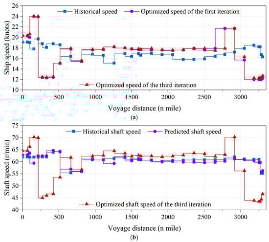
Figure 6.
Optimized speed and optimized shaft speed on route 3. (a) Ship speed. (b) Shaft speed.
5.2. Analysis of Speed Optimization Results under Single Trim and Draft Conditions
Before the ship sails, if the ship trim is not optimized, it is usually considered that the ship trim and draft maintain a single fixed value during the whole voyage in speed optimization, i.e., the adjustment of ship trim and draft is not considered during the whole voyage. In order to be closer to the actual application and eliminate the effect of different trim and draft values on fuel consumption in each segment, a comprehensive speed optimization study is conducted on six routes based on a single trim and draft value. The single trim and draft values of each route are set with reference to the sensor data, with the unstable data which change greatly due to the adjustment of ship trim and draft at the beginning and end of the route excluded, in order to be as close as possible to the trim and draft values of the voyage plan. The comparison results of fuel consumption under single trim and draft conditions after speed optimization are shown in Table 6. In addition, the comparability between the optimized and simulated fuel consumption and the historical fuel consumption in Table 6 is reduced because the trim and draft are single fixed values.
Table 6.
Comparison results of fuel consumption under single trim and draft conditions.
In terms of the difference between the optimized and simulated fuel consumption, the results in Table 6 show that the difference between the two can be reduced to less than 0.1% after at most three optimization iterations, again indicating that the speed optimization iteration algorithm has a fast convergence rate. In terms of fuel-saving rate, it can be seen from Table 6 that compared with the predicted fuel consumption, the fuel-saving rates of optimized and simulated fuel consumption on each route range between 2.4% and 5.0% and between 2.2% and 4.9%, respectively. The results of the case study reveal that the weather loading-speed optimization iterative algorithm based on the turning point-time segmentation method can achieve significant fuel-saving effects.
6. Conclusions
To address the problems of fuel consumption prediction, route segmentation, and weather data loading in ship speed optimization, this study integrates the ET model and PR model based on the idea of model fusion to construct the main engine fuel consumption prediction model and shaft speed prediction model. Based on the construction of the prediction models, an iterative algorithm of ship route segmentation and weather loading-speed optimization is proposed. To verify the effectiveness of the proposed algorithm, a single-objective speed optimization study is conducted on six case routes, and the conclusions are as follows:
- (1)
- The adopted model fusion idea provides a new way for building accurate and reliable fuel consumption prediction and shaft speed prediction models in ship speed optimization. Moreover, the main engine fuel consumption prediction model based on the machine learning method shows significant prediction accuracy, with the relative errors of fuel consumption prediction on six routes all less than 0.9%. The establishment of the shaft speed prediction model provides a reliable way to obtain the optimal shaft speed matching the optimal ship speed, thus improving the practicability and ease of use of the ship speed optimization method.
- (2)
- The proposed route segmentation method and weather loading-speed optimization iterative algorithm reduce the difference between optimized fuel consumption and actual (simulated) fuel consumption, and improve the matching degree between route weather data and optimized speed, as well as the practicability and reliability of speed optimization. In addition, the proposed speed optimization algorithm can achieve a fuel-saving rate between 2.1% and 5.2%, and is a simple but practical and effective speed optimization method in practical navigation planning.
Author Contributions
Conceptualization, X.L. and B.S.; Data curation, X.L.; Formal analysis, X.L.; Investigation, X.L., J.J. and J.D.; Methodology, X.L. and B.S. Software, X.L.; Supervision, B.S. and J.J.; Validation, X.L.; Visualization, X.L.; Writing—original draft preparation, X.L.; Writing—review and editing, B.S., J.J. and J.D. All authors have read and agreed to the published version of the manuscript.
Funding
This research received no external funding.
Institutional Review Board Statement
Not applicable.
Informed Consent Statement
Not applicable.
Data Availability Statement
Not applicable.
Acknowledgments
We thank the three anonymous reviewers for their time spent on this paper and their constructive comments.
Conflicts of Interest
The authors declare no conflict of interest.
Appendix A
To select suitable machine learning methods to construct the ship fuel consumption prediction model and shaft speed prediction model, this study compares the prediction performance of various machine learning methods through modeling experiments. The compared methods include random forests (RF), extremely randomized trees (ET), AdaBoost (AB), gradient tree boosting (GB), support vector regression (SVR), artificial neural network (ANN), ridge regression, LASSO regression, and third-order polynomial regression (PR) methods. The three-layer network structure commonly used in the literature is used in building the ANN model, where the number of neurons in the hidden layer is the same as the number of input features. Furthermore, to ensure the objectivity of the comparison results as much as possible, the Hyperopt library is used to optimize the hyperparameters of each model, with the hyperparameters of each model and the corresponding optimization range shown in Table A1, in which the PR model has no hyperparameters that can be optimized.
Table A1.
Model hyperparameters to be optimized.
Table A1.
Model hyperparameters to be optimized.
| Model | Hyperparameters | Package Reference |
|---|---|---|
| RF | max_depth [2~30], min_samples_leaf [1~20], min_samples_split [2~20], max_features [1~11], n_estimators [10~300], random_state = 7, n_jobs = −1 | scikit-learn |
| ET | max_depth [2~30], min_samples_leaf [1~20], min_samples_split [2~20], max_features [1~11], n_estimators [10~300], random_state = 7, n_jobs = −1 | |
| AB | max_depth [2~10], min_samples_leaf [1~20], min_samples_split [2~20], max_features [1~11], n_estimators [10~300], learning_rate [0.00001~1], random_state = 7 | |
| GB | max_depth [2~10], min_samples_leaf [1~20], min_samples_split [2~20], max_features [1~11], n_estimators [10~300], learning_rate [0.00001~1], subsample [0.4~1], random_state = 7 | |
| SVR | kernel = ‘rbf’, C [0.00001~100], gamma [0.00001~10] | |
| ANN | Activation [‘identity’, ‘tanh’, ‘logistic’, ‘relu’], solver [‘lbfgs’, ‘sgd’, ‘adam’], alpha [0.000001~2], learning_rate_init [0.000001~1], beta_1 [0~0.999], beta_2 [0~0.999], random_state = 7 | |
| Ridge | Alpha [0~10] | |
| LASSO | Alpha [0~10] |
Note: The brackets after the hyperparameter names list the value ranges of the hyperparameters.
The training set is used to build machine learning models and optimize hyperparameters. On the training set, Hyperopt is used to optimize the hyperparameters of the model, and the optimization goal is to maximize the R2 for 5-fold cross-validation. The same number of optimization iterations is used to ensure optimization fairness when optimizing the hyperparameters of different models. Machine learning models with optimal hyperparameters are run on the test set to evaluate the model prediction accuracy, with the fuel consumption prediction accuracy of each model shown in Table A2. Moreover, the variation trend of main engine fuel consumption with ship speed is calculated on some test segments using these models, with the corresponding results of each model shown in Figure A1.
Table A2.
Fuel consumption prediction accuracy of different machine learning models on the test set.
Table A2.
Fuel consumption prediction accuracy of different machine learning models on the test set.
| Model | R2 | RMSE (t/day) | MAE (t/day) | MAPE (%) |
|---|---|---|---|---|
| RF | 0.970 | 2.802 | 1.534 | 2.417 |
| ET | 0.975 | 2.565 | 1.365 | 2.161 |
| AB | 0.971 | 2.787 | 1.592 | 2.495 |
| GB | 0.973 | 2.687 | 1.511 | 2.377 |
| SVR | 0.967 | 2.944 | 1.798 | 2.813 |
| ANN | 0.913 | 4.804 | 3.473 | 5.376 |
| Ridge | 0.827 | 6.781 | 5.062 | 7.780 |
| LASSO | 0.827 | 6.781 | 5.062 | 7.780 |
| PR | 0.927 | 4.414 | 3.234 | 5.026 |
| VR | 0.963 | 3.154 | 2.126 | 3.313 |


Figure A1.
The variation trend of main engine fuel consumption predicted by each model with ship speed. (a) RF. (b) ET. (c) AB. (d) GB. (e) SVR. (f) ANN. (g) Ridge. (h) LASSO. (i) PR. (j) VR.
The model comparison results show that the ET model has the highest prediction accuracy, the PR model has the highest prediction reliability, and the rest of the models have different degrees of disadvantages in both aspects. Therefore, we finally choose to integrate the ET model with the PR model to construct the VR model for fuel consumption prediction, and the results of the VR model also confirm the advantages of model integration.
References
- IMO. Further Shipping GHG Emission Reduction Measures Adopted. Available online: https://www.imo.org/en/MediaCentre/PressBriefings/pages/MEPC76.aspx (accessed on 1 July 2022).
- IMO. Initial IMO GHG Strategy. Available online: https://www.imo.org/en/MediaCentre/HotTopics/Pages/Reducing-greenhouse-gas-emissions-from-ships.aspx (accessed on 1 July 2022).
- Du, Y.Q.; Meng, Q.; Wang, S.A.; Kuang, H.B. Two-phase optimal solutions for ship speed and trim optimization over a voyage using voyage report data. Transp. Res. Part B Methodol. 2019, 122, 88–114. [Google Scholar] [CrossRef]
- Yan, R.; Wang, S.A.; Du, Y.Q. Development of a two-stage ship fuel consumption prediction and reduction model for a dry bulk ship. Transp. Res. Part E Logist. Transp. Rev. 2020, 138, 101930–101951. [Google Scholar] [CrossRef]
- Wang, Z.; Wang, K.; Huang, L.; Chen, J.; Chen, W. Dynamic optimization method of ship speed based on sea condition recognition. J. Harbin Eng. Univ. 2022, 43, 488–494. [Google Scholar]
- Yan, X.P.; Wang, K.; Yuan, Y.P.; Jiang, X.L.; Negenborn, R.R. Energy-efficient shipping: An application of big data analysis for optimizing engine speed of inland ships considering multiple environmental factors. Ocean Eng. 2018, 169, 457–468. [Google Scholar] [CrossRef]
- Wang, K.; Yan, X.; Yuan, Y.; Jiang, X.; Lodewijks, G.; Negenborn, R.R. Study on route division for ship energy efficiency optimization based on big environment data. In Proceedings of the 4th International Conference on Transportation Information and Safety (ICTIS), Banff, AB, Canada, 8–10 August 2017; pp. 111–116. [Google Scholar]
- Psaraftis, H.N.; Kontovas, C.A. Speed models for energy-efficient maritime transportation: A taxonomy and survey. Transp. Res. Part C Emerg. Technol. 2013, 26, 331–351. [Google Scholar] [CrossRef]
- Psaraftis, H.N.; Kontovas, C.A. Ship speed optimization: Concepts, models and combined speed-routing scenarios. Transp. Res. Part C Emerg. Technol. 2014, 44, 52–69. [Google Scholar] [CrossRef]
- Fagerholt, K.; Gausel, N.T.; Rakke, J.G.; Psaraftis, H.N. Maritime routing and speed optimization with emission control areas. Transp. Res. Part C Emerg. Technol. 2015, 52, 57–73. [Google Scholar] [CrossRef]
- Hu, R.X. A route selection and speed optimization method for maritime traffic with emission control areas and weather conditions. Int. J. Sci. 2018, 5, 334–341. [Google Scholar]
- Ma, W.H.; Lu, T.F.; Ma, D.F.; Wang, D.H.; Qu, F.Z. Ship route and speed multi-objective optimization considering weather conditions and emission control area regulations. Marit. Policy Manag. 2021, 48, 1053–1068. [Google Scholar] [CrossRef]
- Wang, S.; Wang, X. A polynomial-time algorithm for sailing speed optimization with containership resource sharing. Transp. Res. Part B Methodol. 2016, 93, 394–405. [Google Scholar] [CrossRef]
- Wang, K.; Yan, X.P.; Yuan, Y.P.; Jiang, X.L.; Lin, X.; Negenborn, R.R. Dynamic optimization of ship energy efficiency considering time-varying environmental factors. Transp. Res. Part D Transp. Environ. 2018, 62, 685–698. [Google Scholar] [CrossRef]
- Yang, L.Q.; Chen, G.; Zhao, J.L.; Rytter, N.G.M. Ship speed optimization considering ocean currents to enhance environmental sustainability in maritime shipping. Sustainability 2020, 12, 93649. [Google Scholar] [CrossRef]
- Tzortzis, G.; Sakalis, G. A dynamic ship speed optimization method with time horizon segmentation. Ocean Eng. 2021, 226, 108840–108853. [Google Scholar] [CrossRef]
- Li, X.H.; Sun, B.Z.; Guo, C.Y.; Du, W.; Li, Y.J. Speed optimization of a container ship on a given route considering voluntary speed loss and emissions. Appl. Ocean Res. 2020, 94, 101995–102004. [Google Scholar] [CrossRef]
- Zhou, T.; Hu, Q.; Hu, Z.; Zhi, J.; Ke, R. Theory and Application of Vessel Speed Dynamic Control considering Safety and Environmental Factors. J. Adv. Transp. 2022, 2022, 5333171. [Google Scholar] [CrossRef]
- Yu, Z.; Wang, H. Real-time optimization of ship energy efficiency based on GWO. Sci. J. Intell. Syst. Res. 2020, 2, 27–33. [Google Scholar]
- Lee, H.; Aydin, N.; Choi, Y.; Lekhavat, S.; Irani, Z. A decision support system for vessel speed decision in maritime logistics using weather archive big data. Comput. Oper. Res. 2018, 98, 330–342. [Google Scholar] [CrossRef]
- Zheng, J.Q.; Zhang, H.R.; Yin, L.; Liang, Y.T.; Wang, B.H.; Li, Z.B.; Song, X.; Zhang, Y. A voyage with minimal fuel consumption for cruise ships. J. Clean. Prod. 2019, 215, 144–153. [Google Scholar] [CrossRef]
- Li, X.H.; Sun, B.Z.; Zhao, Q.B.; Li, Y.J.; Shen, Z.Y.; Du, W.; Xu, N. Model of speed optimization of oil tanker with irregular winds and waves for given route. Ocean Eng. 2018, 164, 628–639. [Google Scholar] [CrossRef]
- Du, Y.; Chen, Y.; Li, X.; Schönborn, A.; Sun, Z. Data fusion and machine learning for ship fuel efficiency modeling: Part III—Sensor data and meteorological data. Commun. Transp. Res. 2022, 2, 100073. [Google Scholar] [CrossRef]
- Berrisford, P.; Dee, D.; Poli, P.; Brugge, R.; Fielding, K.; Fuentes, M.; Kållberg, P.; Kobayashi, S.; Uppala, S.; Simmons, A. The ERA-Interim Archive; European Centre for Medium Range Weather Forecasts: Reading, UK, 2011. [Google Scholar]
- Dee, D.P.; Uppala, S.M.; Simmons, A.J.; Berrisford, P.; Poli, P.; Kobayashi, S.; Andrae, U.; Balmaseda, M.A.; Balsamo, G.; Bauer, P.; et al. The ERA-Interim reanalysis: Configuration and performance of the data assimilation system. Q. J. R. Meteorol. Soc. 2011, 137, 553–597. [Google Scholar] [CrossRef]
- Rio, M.H.; Mulet, S.; Picot, N. Beyond GOCE for the ocean circulation estimate: Synergetic use of altimetry, gravimetry, and in situ data provides new insight into geostrophic and Ekman currents. Geophys. Res. Lett. 2014, 41, 8918–8925. [Google Scholar] [CrossRef]
- Li, X.; Du, Y.; Chen, Y.; Nguyen, S.; Zhang, W.; Schönborn, A.; Sun, Z. Data fusion and machine learning for ship fuel efficiency modeling: Part I—Voyage report data and meteorological data. Commun. Transp. Res. 2020, 2, 100074. [Google Scholar] [CrossRef]
- Geurts, P.; Ernst, D.; Wehenkel, L. Extremely randomized trees. Mach. Learn. 2006, 63, 3–42. [Google Scholar] [CrossRef]
- Pedregosa, F.; Varoquaux, G.; Gramfort, A.; Michel, V.; Thirion, B.; Grisel, O.; Blondel, M.; Prettenhofer, P.; Weiss, R.; Dubourg, V. Scikit-learn: Machine learning in Python. J. Mach. Learn. Res. 2011, 12, 2825–2830. [Google Scholar]
- Bergstra, J.; Yamins, D.; Cox, D. Making a science of model search: Hyperparameter optimization in hundreds of dimensions for vision architectures. In Proceedings of the 30th International Conference on Machine Learning, Atlanta, GA, USA, 16–21 June 2013; pp. 115–123. [Google Scholar]
- Bennett, G. Practical rhumb line calculations on the spheroid. J. Navig. 1996, 49, 112–119. [Google Scholar] [CrossRef]
- Aertssen, G. Service performance and trials at sea. In Proceedings of the 12th International Towing Tank Conference, Rome, Italy, 22–30 September 1969; pp. 210–214. [Google Scholar]
Publisher’s Note: MDPI stays neutral with regard to jurisdictional claims in published maps and institutional affiliations. |
© 2022 by the authors. Licensee MDPI, Basel, Switzerland. This article is an open access article distributed under the terms and conditions of the Creative Commons Attribution (CC BY) license (https://creativecommons.org/licenses/by/4.0/).