Article

Simulating the Interconnected Eastern Mediterranean–Black Sea System on Climatic Timescales: A 30-Year Realistic Hindcast

Department of Marine Sciences, School of the Environment, University of the Aegean, 81100 Mytilene, Greece
*
Author to whom correspondence should be addressed.
J. Mar. Sci. Eng. 2022, 10(11), 1786; https://doi.org/10.3390/jmse10111786
Submission received: 16 September 2022 / Revised: 11 November 2022 / Accepted: 14 November 2022 / Published: 20 November 2022
(This article belongs to the Special Issue Hydrodynamic Circulation Modelling in the Marine Environment)

Abstract

:
Inter-basin water exchanges can be quite important in climatic-scale numerical studies simulating the circulation and hydrographic characteristics of neighboring oceanic basins connected through narrow straits. The crucial role of the interaction between the Mediterranean and the Black Seas is often overseen in simulations, which rely mostly on parameterizations to describe the exchange, essentially decoupling the two basins. In this study, the fully interconnected Eastern Mediterranean–Black Sea system is simulated for the historical period (1985–2015) using realistic boundary conditions (lateral, atmospheric and hydrological), with a hydrodynamic fully three-dimensional ocean modeling system. The setup of such a configuration is thoroughly described and the performance of the 30-year hindcast product is validated exhaustively against observations and model results, by evaluating the representation of surface fields, circulation, three-dimensional hydrographic characteristics, volumetric water exchanges, and the spatio-temporal variability of the above. The comparison shows exceptional performance, minimal drift, and substantial improvement compared to modeling studies that do not include the interaction. Moreover, due to the free-run configuration of the simulation (i.e., absence of assimilation schemes) no additional input is required other than the respective boundary conditions, making it possible to reliably extend the same setup for scenarios where observational data are not available, such as in future projections.

1. Introduction

The Mediterranean and the Black Seas constitute two neighboring and communicating marine basins which correspond to two contrasting textbook examples of a concentration and a dilution basin, respectively, regarding their thermohaline functioning and overturning circulation [1]. Thus, the Mediterranean exports dense water to its neighboring basins, while the Black Sea exports light, brackish water to the Mediterranean. The strongest signature of this contrasting behavior is recorded in the water exchange between the two basins through the system of the Bosphorus Strait, Marmara Sea and Dardanelles Strait (also often referred to as the Turkish Strait System, TSS), where the impressive intensity, stability and contrast between the surface and subsurface currents provided the stimulus to Count Luigi Ferdinando Marsigli in 1685 to found modern physical oceanography by attributing the exchange flow to the contrasting salinity of the two basins [2].
The important role of connecting straits in determining the oceanographic characteristics of the Mediterranean has been described in the past through several works (e.g., [3,4,5]). The Gibraltar exchange is almost two orders of magnitude higher than the exchange through the TSS, thus at first glance it appears that the latter can be ignored in either long-term hindcasts or climatic projections of the Mediterranean circulation. And indeed, this would be the case if the Aegean Sea, first receptor of the Black Sea waters into the Mediterranean, would not also be an alternative (to the Adriatic) source of Eastern Mediterranean Dense Waters [6,7]. The inflow of Black Sea waters (BSW) in the north Aegean tends to hinder dense-water formation in the following ways: (a) the lateral buoyancy inflow (in the form of light BSW) locally reduces surface density and increases upper water-column stratification and (b) the much lower temperature of BSW relative to the underlying Aegean/Levantine water masses drastically reduces heat losses from the sea to the atmosphere in the winter [8]. The North Aegean Sea (despite being a continuous buoyancy importer from the Black Sea) has been reported as the triggering region for the massive Eastern Mediterranean Transient event (hereafter EMT) [9,10]. Therefore, the exchange through the straits is considered a regulating factor of the Aegean Sea buoyancy budget and, consequently, of the overturning circulation of the Eastern Mediterranean Sea [9]. Although the relative importance of the role of the reduced buoyancy inflow through the Dardanelles in initiating the EMT has been challenged [11], it is clear that a good representation of the exchange through the TSS is required for the successful reproduction both of the vertical structure of the water column in the North and Central Aegean Seas, as well as the buoyancy budget (and thus the overturning processes) of the region. As the interannual variability of the exchange was gradually realized, more recent simulations of the North Aegean circulation have evolved from using parameterizations of the seasonal cycle of the exchange [12,13] to exploiting the water budget of the Black Sea [14].
The existing literature on numerical studies simulating the interconnected Eastern Mediterranean–Black Sea basins as a fully-coupled three-dimensional hydrodynamic system may be categorized into two broad categories based on spatio-temporal extent and resolution. In one category, studies that mainly focus on simulating the exchange and hydrodynamics at the straits (e.g., [15,16,17,18,19], to mention a few). These studies usually feature high-resolution, structured or unstructured mesh grids, implementing either hydrostatic or non-hydrostatic modeling systems with various vertical discretization schemes. Many of these implementations resolve the flow with impressive accuracy and realism, nevertheless, their high computational demands apply restrictions to either the simulation period (i.e., few months to a few years), the extent of the integration domain (i.e., regional to the straits), or both. The second category comprises of studies that simulate part of the system in climatic scales (i.e., tenths of years) either as a hindcast, a future projection or both (e.g., [4,20,21], and most simulations in [22] except one (namely [23])—see below). These studies simulate the Mediterranean Sea for longer periods of time, and use parameterizations for the exchanges at the Dardanelles and Bosphorus straits instead of numerically solving the flow. This is accomplished through various methods, some of which include imposing a seasonal cycle (deduced either from short-term observations, or short-term simulations), treating the straits as an open boundary source/sink of water, using the basins’ water budget to calculate flow rates (i.e., LOICZ method), etc. This second category also includes studies that simulate the fully interconnected domain, but do so only in a two-dimensional or barotropic sense, for example surface wave or tidal dynamics simulations (e.g., [24]). Very few studies fall outside of these two categories, namely, the recent [25], which resolves the whole system at a short-term (5 days forecast—14 days overall) operational level while not providing validation results for the Black Sea, [23] which resolves the whole system, but in very low resolution, especially in the Eastern Mediterranean/Black Sea (almost similar to that of a GCM), thus considered of low accuracy, and the recent [26], which is the only equivalent to our study (temporally and spatially), includes the whole Mediterranean and Black Seas and resolves the whole system in climatic scales. However, the validation of model performance in this recent study focuses mostly on surface fields (namely, Surface Height, Surface Temperature and Surface Salinity) and no validation results are provided for the Black Sea.
The majority of the above approaches fail to replicate the climatic behavior of the basin in a holistic fashion; in the first category of studies because of limits in coverage, temporal extent and boundary conditions, and in the second category because of the reduced variability of water characteristics in the exchange. This is expected to have a greater impact on model skill at regions closer to the exchange location (i.e., the Aegean Sea, the straits system and the benthic portion of the Black Sea), and becomes conspicuous when examining the temporal evolution of these water characteristics. Moreover, any climate-change-related signal that may exist in either basin is not conveyable to the other, limiting the ability of such setups as future projection tools. As an example of such a chain of events, a projected future precipitation anomaly over the Black Sea catchment area would affect the long term volumetric inflow of fresh water in the basin, changing the water characteristics of surface water inflow in the Aegean Sea, which would in turn affect the air–sea interaction through energy fluxes, and the thermohaline composition and functioning in a local sense as well as in the wider eastern-Mediterranean region.
Despite the emerging importance of regarding the Black Sea–Mediterranean Sea basins as an interconnected oceanographic system, the necessity of using very high resolution grids to resolve the flow at the straits increases the numerical cost and in some cases renders such approaches prohibitive for long-term simulations. This is apparent in the scientific literature; with the exception of the aforementioned [23,26], no other studies exist up to date that simulate the interconnected system as a whole for climatic periods of time, either in a historical or future projection sense. Aiming to an improved tool for climatic studies of the Aegean Sea, we have suitably designed a model set-up for the whole Mediterranean–Black Sea system. As a first application, a 30-year-long hindcast (covering the period 1985–2015) has been produced, and the results are presented here in the form of an extended validation of the simulation. Simulations like this might suffer from several factors, a common one (apart from numerical instabilities) being numerical drift. Numerical drift refers to the gradual increase or decrease over time of a quantity or variable (e.g., Temperature, Salinity, ssh) at a specific region or even throughout the whole domain, which is clearly distinguishable from the inherent interannual variability of the system. This can occur in simulations with large or diverse domains, especially when using low resolution boundary conditions and/or when the model is integrated over time for long periods with no intervention (i.e., data assimilation). Special care has been taken during the model configuration and grid construction process, to minimize numerical drift and to produce a tool capable of simulating long periods of time reliably, without the use of data assimilation schemes.
The present study addresses the aforementioned issues and introduces a simulation product that can realistically describe the climatology and physical oceanography of the Eastern Mediterranean with emphasis on the Aegean Sea (the region directly affected by the basin exchange), in terms of water transport, water characteristics, energy budget and buoyancy fluxes. Moreover, the dataset should cover the 1985–2015 historical period for validation and reanalysis purposes, while also having the capability of extending into the future for the exploration of climate-change-related scenarios in the wider region. The innovation of this modeling system lies within its ability of simulating processes in the interconnected system, as well as its capacity of being extended into the future with minimal intervention.

2. Materials and Methods

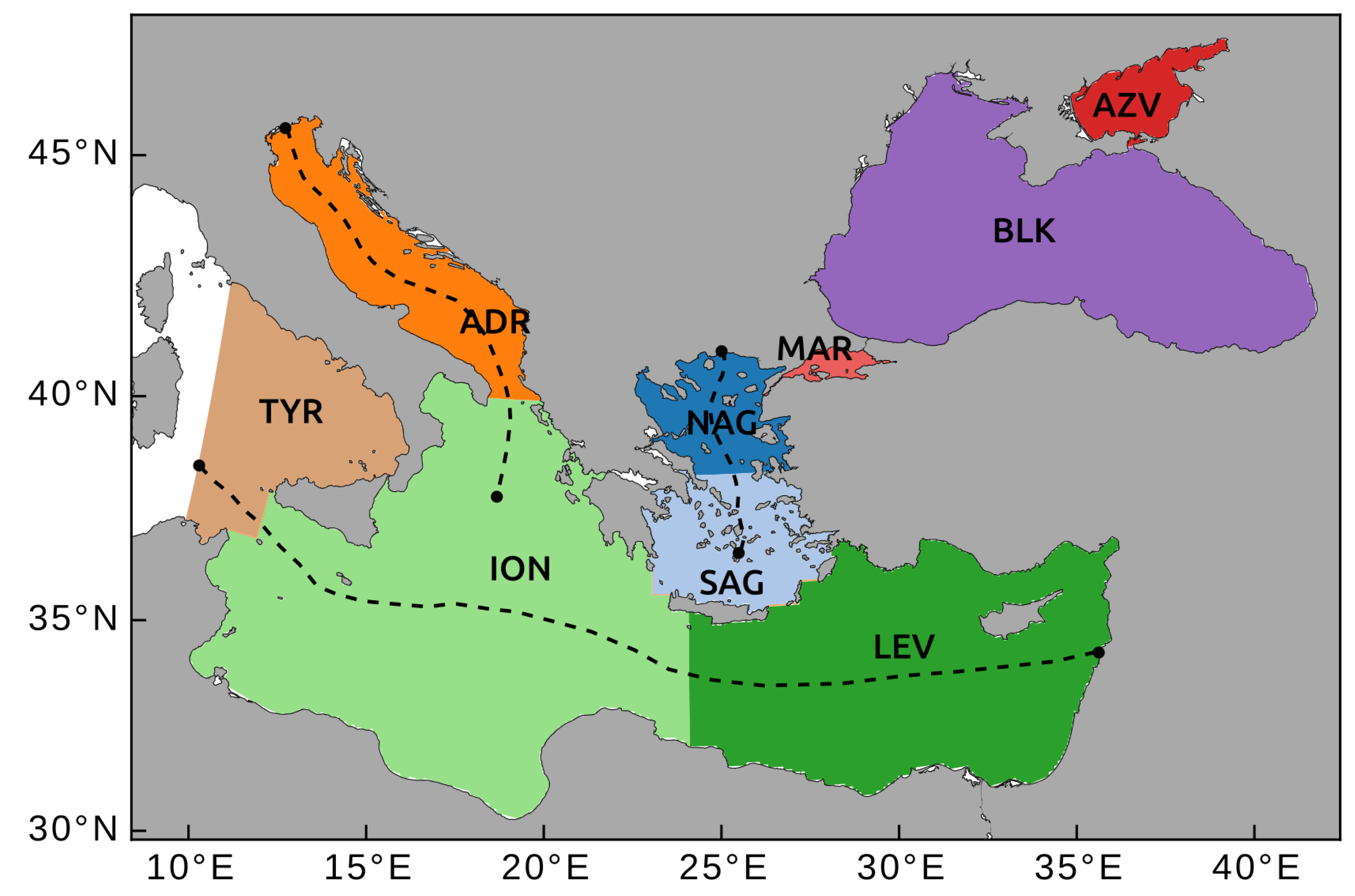
2.1. Domain Selection and Model Setup

The modeling system of choice for this simulation was the Regional Ocean Modeling System (ROMS) [27,28], a free–surface, hydrostatic, primitive equation model, featuring a highly versatile code with numerous vertical and horizontal mixing and advection schemes, as well as a terrain-following sigma coordinate system for the vertical levels.
The primary objectives of the model setup was to develop a product that (a) is able to simulate the physical characteristics of the Aegean Sea and their long-term climatic variability, as well as potential changes of those in a changing climate, while resolving interactions with the Black Sea that take place through the narrow straits of Bosphorus and Dardanelles; (b) can do so for long decadal-scale simulations without the need for corrective interventions (such as data assimilation or relaxation methods), giving it the ability to be used as both a historic simulation as well as a future projection tool; (c) does not require very high-frequency oceanic boundary conditions; and (d) is not excessively demanding of computational resources.
The above requirements determine to a large degree the simulation domain. In order to be able to dynamically reproduce potential future changes in the interaction between the Aegean and the Black Seas or its variability, an adequate simulation of the water properties of the two basins is needed alongside the resolution of the volumetric exchange between them. The Black Sea is a water body whose physical characteristics are strongly affected by the inflow of riverine water by major rivers draining through its very large catchment area, spanning a considerable part of central/eastern Europe and western Asia. Therefore, any potential future change in the riverine water volume inflow into the basin (either anthropogenic or not), would need to be accounted for in the simulation. This dictates the inclusion of the Black Sea and the components of its hydrological cycle in the model setup. Furthermore, an open boundary at the southern end of the Aegean would render the region of interest directly dependent on the quality of boundary conditions. Hence, although the above was not an issue for historical data, it was decided as part of planning ahead to set the open boundary further west at roughly the longitude of Sardinia, using the Tyrrhenian Sea as a buffer in order to be able to use lower resolution (either temporal-wise or spatial-wise) boundary condition data for the future projections. This would also provide a larger simulation area, giving the opportunity to follow the signature of water masses entering and leaving the Aegean basin, while rendering the whole eastern Mediterranean/Black Sea region a single, compact and closed simulation system with only one and relatively short open boundary at the west. The geography of the domain, as well as the definition used here for the individual sub-basins, is presented in Figure 1.
The grid was constructed in a curvilinear-coordinate geometry with a variable size, in order to better describe the relatively diverse and convoluted coastline of the eastern Mediterranean/Black Sea basins. Studies of straits in the Mediterranean Sea demonstrate that the Bosphorus and Dardanelles hydrodynamic regime is further away from the hydraulic-control limit and closer to the viscous–advective–diffusive form limit, when compared to the Gibraltar strait [15,29,30,31]. A past study [30] shows that a detailed description of processes in the straits system requires the use of a non-hydrostatic model of very high spatio-temporal resolution, providing the ability to reproduce the intensity of hydraulic jumps in the straits. However, the present work investigates the extent to which a hydrostatic model is able to reproduce the hydrographic impact of the exchange on the neighboring basins over climatic time scales. To that aim, the gridline density was increased at those regions, leading to a final grid size ranging from around 5–7 km in areas of lower hydrodynamic requirements, to around 1.2 km at the straits, with an average size of 3 km for the whole simulation area. In this approach, the straits’ resolution ranges from five grid cells in wider sections, down to one grid cell at their narrowest points, which in combination with the bathymetry presents a realistic topographic restraint to the flow, and can reasonably simulate—as will be shown—the long term water exchange and water properties’ advection, as well as their seasonal variability, for long-term studies. The geometry of the grid is presented in Figure 2, and the grid sizes for each basin in Table 1. The downsides of such a configuration is the deformation of the grid, and the relatively low resolution at the Northern Adriatic, the Azov Sea and at the Southern-most portion of the domain.
Previous experience in modeling the Aegean Sea has shown that boundary over-specification can propagate biased tracer and velocity-field values into the simulation domain. At the open boundary in the west, a sponge layer of 10 grid points of increased viscosity and diffusivity values was used to provide a buffer zone and avoid this issue. Throughout the rest of the domain, horizontal mixing is additionally adjusted, by linearly scaling around diffusivity and viscosity coefficients’ default values, with respect to grid cell area. Data output from the buffer zone is masked-out from the analysis.
In the vertical, 30 sigma coordinate levels of variable resolution where used, following the bathymetry provided by the 30 arcsecond General Bathymetric Chart of the Oceans (GEBCO) 2014 database [32], for the region of interest. In order to ensure the hydrostatic consistency of the grid and avoid pressure gradient errors, the bathymetry was smoothed via a direct iterative method [33] until rx0 [34] and rx1 [35] reached values of 0.13 and 7.39, respectively. The baroclinic timestep was 60 s with 20 barotropic timesteps in between, bringing the maximum barotropic Courant Number down to 0.56.
For the vertical mixing parameterization, the Mellor and Yamada level 2.5 closure scheme was chosen [36,37,38], together with the Kantha and Clayson [39] stability function formulation for further flexibility. The model’s default background values ( 5 × 10 6 m 2 s 1 ) were used for vertical viscosity and diffusivity. For the horizontal mixing, a harmonic Laplacian operator was selected for diffusion and viscosity. A quadratic drag law was used for the parameterization of bottom stress and a free-slip condition along the horizontal boundaries. The default third-order upstream scheme was used for the advection of momentum, and the recursive-flux-corrected MPDATA algorithm for the advection of tracers, with a further limiter in upwind corrector fluxes for stability [40].
A combination of boundary conditions were used for the open lateral boundary at the west; more specifically, Chapman boundary conditions for the free-surface elevation [41], an adaptive radiation-nudging condition for the 3D velocity and tracer fields [42], and the so-called Shchepetkin (or Flather) condition for the barotropic velocity field [43,44]. The Sea of Azov was included in the grid setup, with the intention of it functioning as a pre-mixing zone for the water inflow of Don and Kuban rivers into the Black Sea. This was designed in order to provide a more realistic representation of the water characteristics exiting the strait of Kerch, than what would result by assigning a point source at the strait. Moreover, it eliminates the need of oceanic boundary conditions in the Black Sea. Apart from the aforementioned functioning, Azov Sea fields are not considered part of the simulation and are excluded from the analysis. This is done mainly because of the relatively coarse resolution of the grid in this shallow basin, combined with considerations regarding realism of the topography/bathymetry at the strait.
Initial conditions were only provided for temperature and salinity (see Section 2.2), so a spin-up process was performed for the free-surface and velocity fields. A continuous 1985 year was used in a loop of two years, until the total kinetic energy of the model was stabilized (i.e., fluctuated around a value). The simulation was then initiated from the 1 January 1985, and ran for 30 years. Model output included daily averages for several relevant variables, among them tracers, barotropic and 3D velocity fields, density, heat and salt fluxes, energy fluxes, all of which were considered valuable for dynamic or climatic studies.
Special effort was put to keep the simulation as close to realistic conditions as possible. This would ensure that the hindcast can be used for climate analysis, and reproduces the climatic variability of the water characteristics and derivative physical parameters of the oceanography of the region. To that aim, realistic atmospheric forcing, open boundary conditions, river inflow data as well as initial conditions were chosen from well-established reanalysis/modeling studies (see Section 2.2) as external/forcing conditions. The model ran for a 30-year period from 1 January 1985 to 31 December 2014.
Finally, neither data assimilation schemes nor relaxation methods were employed during the simulation; this ensured that the same configuration could be used for future projections, using a reproducible setup without major changes and consequent loss in model confidence.

2.2. Realistic Forcing

The simulation was run under realistic atmospheric forcing from the ECMWF–ERA interim reanalysis dataset. The temporal resolution was 3-hourly, and the spatial resolution for all fields was 0.125 ° × 0.125 ° (which is provided in essence as an offline-upscaled version from 0.75 ° × 0.75 ° ). For a more realistic reproduction of the diurnal cycle, accumulated values were used, while fluxes of momentum and heat from the atmosphere into the ocean were derived using bulk flux parameterization [45]. The shortwave radiation flux was distributed among the surface/upper layers, using an absorption function dependent on the optical properties of the water following specific Jerlov water types [46], as this has a significant influence on vertical mixing dynamics. The Black, Azov and Marmara seas, along with the Bosphorus strait, were all assigned the eighth Jerlov water type (Black Sea), while the Dardanelles and the rest of eastern Mediterranean were assigned the second Jerlov water type (Mediterranean Sea).
Lateral boundary conditions for salinity (S), temperature (T), sea surface height ( ζ ) and velocity field (u,v) at the western boundary were calculated from daily averages of the Mediterranean Forecasting System at 0.0625 ° × 0.625 ° resolution and 72 vertical z-coordinate levels [47,48]. The dataset covers the period between 1 January 1985 to 31 December 2014. Initial conditions for salinity and temperature for 1 January 1985 were constructed through bi-linear interpolation of the SeaDataNet II–MEDAR/MEDATLAS II project’s observational dataset [49,50].
Riverine daily volumetric inflow data (including water temperature) were introduced for rivers within the simulation regime. Over-definition of river sources could introduce numerical noise in a disproportional degree to the added realism, so only nine major rivers with the largest average volumetric flow rates were included; Danube, Dnieper, Dniester, Don, Kuban, Red and Sakaraya in the Black Sea, and Po and Nile in the Mediterranean. For the first eight rivers draining from the European and Asian continents, data were provided from the results of the E-HYPE hydrological model of the Swedish Meteorological and Hydrological Institute (http://hypeweb.smhi.se, accessed on 28 January 2018) [51], and the dataset consists of daily volumetric flow and temperature values. For the Nile river, data were provided by the University of New Hampshire—Global Runoff Data Center—Composite Runoff Fields V1.0 (https://www.compositerunoff.sr.unh.edu, accessed on 28 January 2018), as monthly volumetric flow climatology, which was then temporally interpolated to daily values. In general, water with salinity values between 0.5 and 30 is considered brackish, while the average salinity of world’s riverine water is around 0.12 [52]. This value can be much higher close to the river mouth due to sea water intrusion [53]; in this simulation, the salinity of all riverine water entering the domain was set to a constant value of 5, which apart from being realistic (given the cell area), also helped to avoid numerical instabilities.

2.3. Validation Datasets

Sea surface temperature data (SST) at a resolution of 0.05 ° × 0.05 ° , from the CMEMS reprocessed Mediterranean SST dataset and the CMEMS reprocessed Black Sea SST dataset, were used as part of the model’s performance validation process [54,55,56]. Both datasets consist of daily SST fields fully covering the 30-year simulation period. The EMBS field was bi-linearly interpolated to the reprocessed satellite one. Estimated error standard deviation from the reanalysis process of converting satellite-swath data to a gridded dataset (mostly attributed to errors due to optimal interpolation of level 3 to level 4 data, and cloud-coverage-related uncertainties), is included in the CMEMS product and was used as a filtering variable for excluding data of lower quality. For each cell, days with an estimated error standard deviation larger than 0.5 were excluded, and monthly averages were then calculated for the comparison. Data for the Marmara Sea are absent in the CMEMS product, so this region is excluded from the comparison.
The all-satellites European Seas Gridded SSALTO/DUACS Sea Surface Height Level-4 product and derived variables altimetry was used for the validation of sea surface elevation [57], also referred to hereafter as the AVISO dataset; the dataset covers the period from 1993 to 2014. Again, because of the higher resolution of the EMBS model compared to the altimetry dataset, the former was bi-linearly interpolated to the latter, and monthly averages were calculated for the comparison. The AVISO dataset output includes the variables Absolute Dynamic Topography (ADT), Sea Level Anomaly (SLA), and geostrophic current velocities. The relation between these variables is that ADT is the sum of Mean Dynamic Topography (MDT) and SLA. The relevant output variable from the ROMS modeling system that can be used for comparison is sea surface height zeta ( ζ ), and here there are two considerations to be made. Firstly, regarding the datum of surfaces in the two datasets, AVISO’s ADT reference surface is the geoid, while in ROMS the default reference surface for ζ is depth-level zero (i.e., the sea surface of the computational domain at rest). It was decided to use this default configuration during the simulation, as the two surfaces can be offset to the same datum in post-processing by subtracting the spatial-mean of MDT from the local ADT. The second consideration is with respect to the steric effect (inverse barometer effects are present in both the AVISO and ROMS datasets, and is further discussed in Section 4). While ADT in altimetry includes the contribution of steric effect (differences in surface height due to expansion or contraction of the water column), in ROMS the steric height is not included in ADT. Nevertheless, our calculations suggest that steric effect contribution is very small (less than 5% of SLA), so it is considered adequate for the purposes of the present validation to directly compare ADT from altimetry with ζ from the numerical model. Nevertheless, because of differences in the datum as mentioned above, surfaces in both datasets need to be centered around a common level (by subtracting the mean value). Due to the large extent of the simulation basin, considerable spatial variability in ADT exists for both the simulation and the satellite datasets, making local variability challenging to discern. For this reason the comparison is performed in two ways. In a first approach, maps of temporally averaged ADTs for both simulation and satellite data, are centered around zero for specific sub-basins by subtracting the spatiotemporal mean of that basin, and then the comparison is performed. This gives a better overview of the simulation performance regarding elevation of the sea surface itself, in specific areas. In the second approach, the horizontal gradient of the sea surface ζ , and the barotropic component of geostrophic velocities are calculated by:
h ζ = ζ x ı ^ + ζ y j ^ , u g = g f ζ y , v g = g f ζ x ,
which makes possible the simultaneous comparison over the entire domain.
The validation of simulated volumetric water exchange through the straits is performed through the use of two datasets. One dataset comes from a theoretical study that employed a chain of hydraulic control Strait models and 1.5-dimensional ocean basin models to calculate water fluxes between the Black Sea and the Aegean Sea through the Dardanelles and Bosphorus straits [58]. These fluxes are given in daily values for the period 1985–2009, at both straits for the upper and lower layer; the upper or surface layer refers to the waters moving from the Black Sea towards the Aegean Sea, while the lower or bottom layer refers to the waters moving in the opposite direction. This dataset has been employed in previous numerical studies as boundary conditions, when the inclusion of the straits in the domain was not possible [59,60]. The second dataset used for the validation comes from a study that used direct current velocity observations at the Dardanelles strait, to infer volumetric transport through the cross-sectional area of the strait [61]. It is given in hourly values from 1 September 2008 and 31 August 2009. To calculate volumetric transport from the EMBS simulation current velocities, the product of each layer’s cross sectional area with the normal velocity vector was taken, then for each gridbox the depth at which velocity changed direction with respect to channel direction was used as the division between the upper and lower layers, and the sum of transport was calculated for the two layers. In addition, seasonal averages of salinity and temperature were calculated along a vertical transect running from the exit of Bosphorus in the Black Sea through the Sea of Marmara and to the exit of Dardanelles in the Aegean Sea, following the same routing as in [62], in order to examine whether the thermohaline composition patterns of the exchange at the straits are reproduced realistically when compared to hydrographic observations ([62,63]).
In order to perform a thorough and complete validation of hydrodynamic data, the entire three-dimensional domain needs to be examined. More specifically, a realistic ocean simulation is one that can adequately reproduce not only the surface or two-dimensional fields, but the entire water column. For this reason, observational datasets from oceanographic surveys describing temperature and salinity within the water column were extensively used during the model validation process. Data were provided from the MEDAR/MEDATLAS II and SeaDataNet II projects, forming a comprehensive collection of all available data from water column profile casts (CTDs, ARGO floats, etc.) for the Mediterranean and Black Seas [49,50]. The available quality control of the datasets was used to include only top-grade casts; i.e., in a quality scale from 1 to 4, only casts that consisted of quality 1 data in at least 95% of the water column were selected. Preparation included making the vertical level quantization of the model (being in sigma coordinates) and that of the cast profiles relevant, by interpolating them to standard oceanographic depth levels. It is usual for simulation products to exhibit small or even large deviations from observations, making it difficult to judge and quantify whether a simulation performance is as good as it could be. Naturally, there is an upper limit in the realism one could expect from a model, so as an additional tier in this validation process, we include in the comparison results from operational forecasting systems in the Mediterranean and Black Seas, featuring state-of-the-art assimilation and surface-relaxation methods, thus making them as realistic as possible. This is done in an effort to designate the upper performance limit for a simulation like EMBS, which is of similar resolution and setup, but runs without data assimilation. Moreover, such a comparison can showcase the importance of including the hydrodynamic interaction at the straits. The systems used for this reason here, are the Physical Reanalysis components of the Mediterranean Forecasting System (MFS) [47,48], and the Black Sea Monitoring Forecasting Center (BS-MFC) [64,65]. The MFS resolution is 1/16° with 72 vertical levels, and the simulation period is covering the range of the EMBS simulation (from 1985 to 2014), although years 1985 and 1986 are considered a spinup and were only obtainable through personal communication with the authors. The BS-MFC resolution is 1/36° × 1/27° with 31 vertical levels, and covering the period from 1993 to 2014. The modeling system for both MFS and BS-MFC is the Nucleus for European Modeling of the Ocean (NEMO), and a three-dimensional variational data assimilation scheme (OceanVar) was used for temperature and salinity profiles, satellite Sea Level Anomaly along track data and satellite SST data assimilation. Simulated (EMBS) and control-simulation (MFS/BS-MFC) vertical profile data are calculated at the same time and place as the observed survey profiles (MEDATLAS), and spatiotemporal averages as well as their variability are calculated and compared for the whole period within smaller areas (e.g., North Aegean Sea, Ionian Sea, etc.), in terms of average profiles.

3. Results

The validation of the EMBS simulation performance is done in five steps. In the first two steps, surface fields (namely Sea Surface Temperature and Sea Surface Elevation) are validated against satellite observations. In the third step, a timeseries of the volumetric water exchange at the straits is compared to theoretical as well as observational studies, while seasonal averages of tracers in along-strait cross-sections demonstrate the distribution of water characteristics within the straits. In the fourth step, the general circulation both in terms of horizontal surface and subsurface currents, as well as in terms of the zonal and meridional overturning streamfunctions, is compared to known circulation patterns of the region. In the fifth step, vertical profiles of Salinity, Potential Temperature and Potential Density Anomaly are compared to both observations and state of-the-art operational assimilated model results.

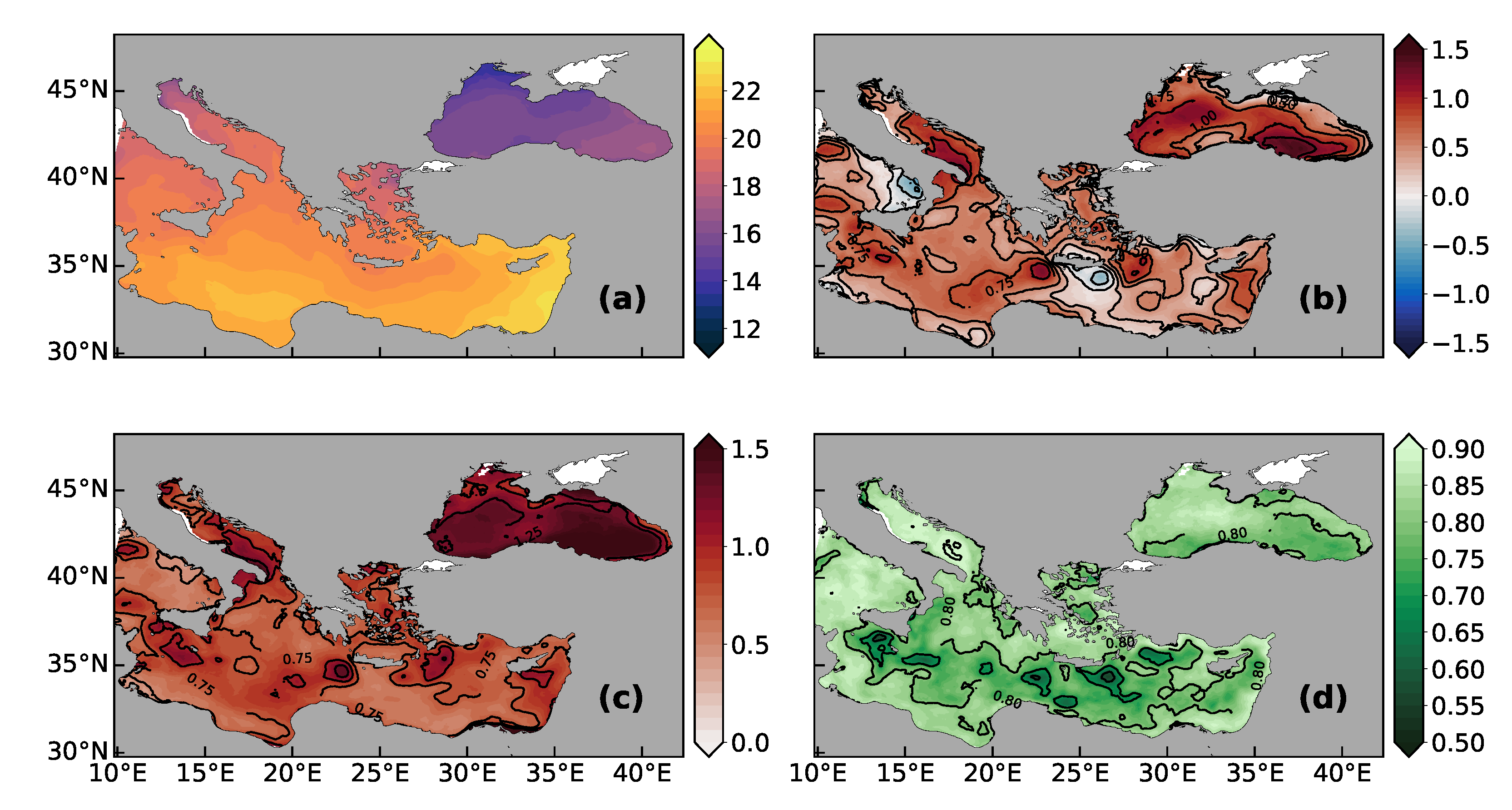
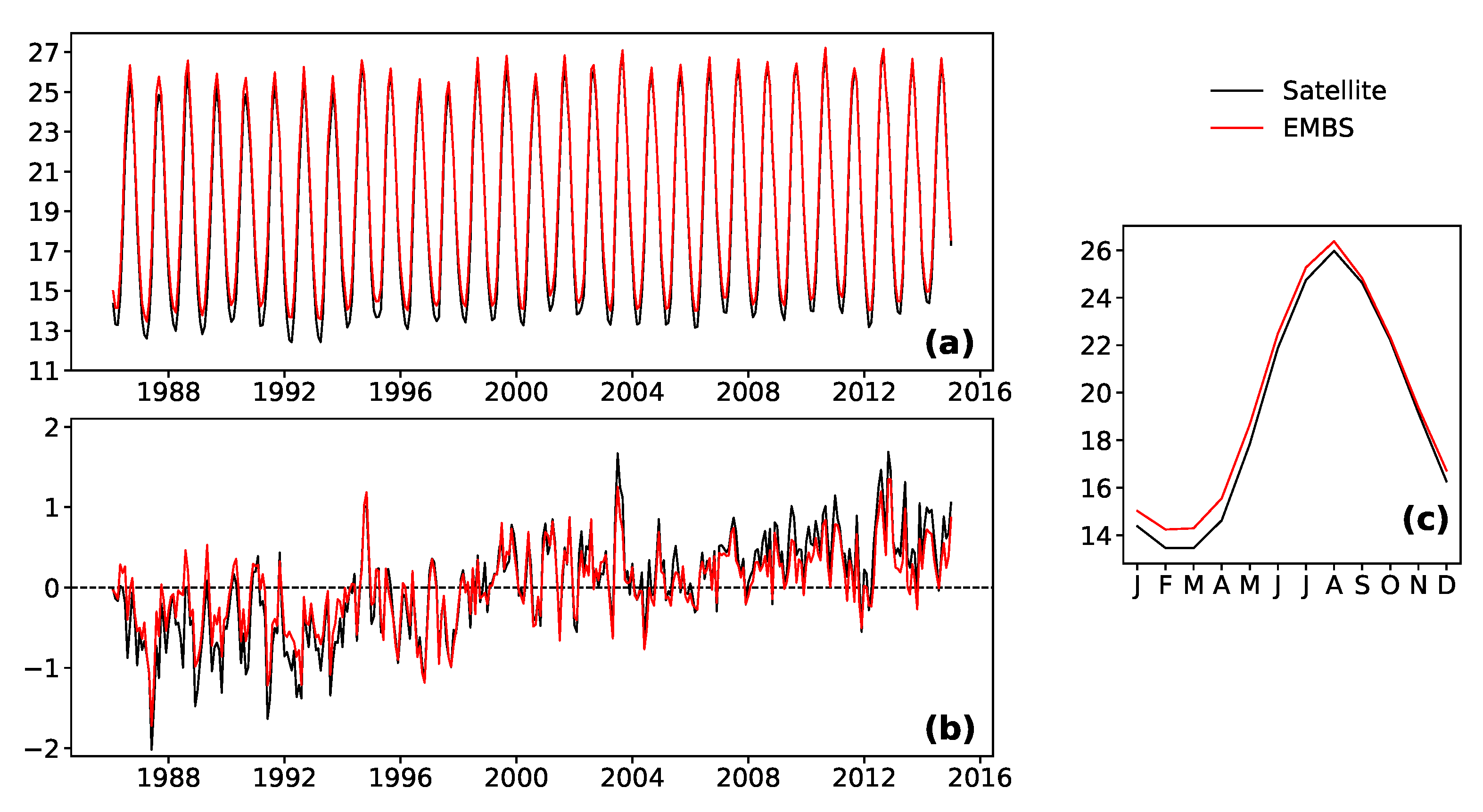
3.1. Sea Surface Temperature

In this first step of the validation process, we compare monthly-averaged SST observations in the form of level-4 Satellite-data reanalysis (AVHRR), to results of the EMBS simulation. The spatial variability of SST, as observed by satellite, is closely reproduced by our simulation (Figure 3). Bias over the whole domain is close to 0.55 °C, with largest bias/RMSE appearing in the Black Sea and lowest appearing in the Levantine Sea (Table 2). Regions of more significant deviation include areas of mesoscale gyres (see Figure 3b), like the Cretan cyclone (bias∼+0.85 °C) and Ierapetra anti-cyclone (bias∼–0.50 °C), the southernmost part of the Adriatic Sea (bias∼+0.75 °C), the eastern-southeastern part of the Black Sea (bias∼+1.25 °C), and the coastal area between the Nile river and Suez canal (bias∼+1.00 °C). The correlation between satellite and simulated SST’s, as described by Peason’s correlation coefficient, is above 0.98 for the whole domain due to the strong influence of the seasonal cycle. The same metric for the deseasoned signal shows high correlation of over 0.7 between simulated and observed SST’s for the whole domain (Figure 3d).
The domain-averaged temporal evolution of SST showcases the seasonal cycle as the most prominent source of variability in the timeseries (Figure 4), with the aforementioned overestimation of 0.55 °C for the simulation, emerging systematically on the seasonal cycle (Figure 4c). The temporal variability of SST is reproduced accurately, with the deseasoned 1985–2014 simulated timeseries closely following the deseasoned satellite observations (Figure 4b). The basin-wide long-term warming trend is underestimated, with 0.046 °C/yr for the satellite and 0.030 °C/yr for the simulation, both of which were tested for statistical significance with the Mann–Kendall test (with resulting s-values > 0, and p-values < 0.01).

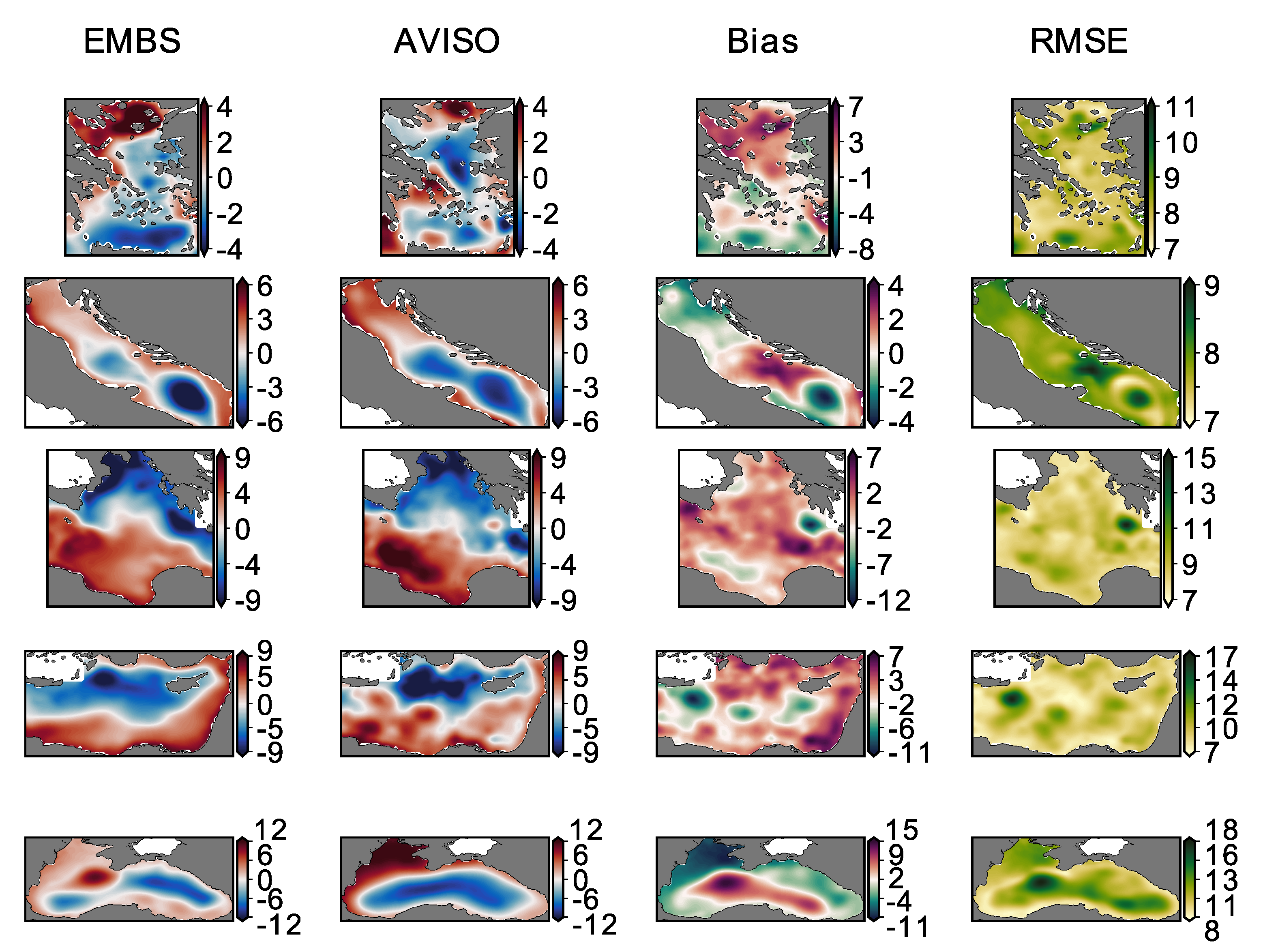
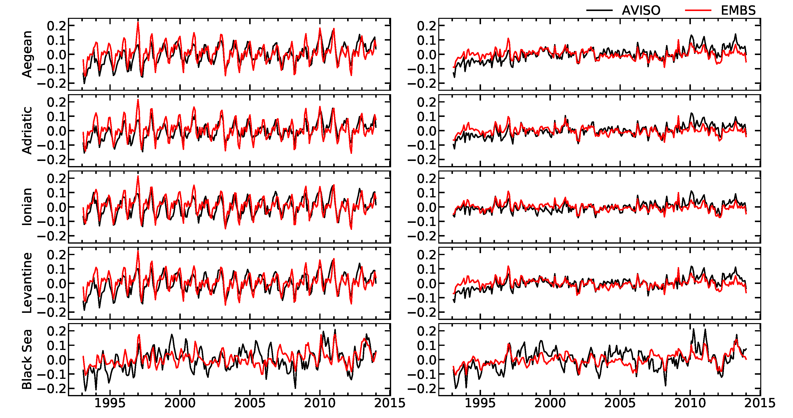
3.2. Sea Surface Elevation

A comparison of ADT as described in Section 2.3, between the EMBS simulation and satellite data for different sub-basins of the domain, can be seen in Figure 5. ADT in this analysis is zero-centered, meaning that the mean value is removed, which is almost the equivalent of moving the datum to zero meters. The overall shape of the sea surface for the period 1985–2014 closely resembles the one described by the satellite altimetry reanalysis product (AVISO). In combination with Figure 6, it can be seen that large and known elevation/flow patterns of the Mediterranean, are being reproduced qualitatively as well as quantitatively. More specifically, flows like the anti-cyclone of the North Aegean, the cyclone of the central Aegean and the front created by the Dardanelles outflow, the mid-Adriatic and south-Adriatic pit cyclones as well as the east and west Adriatic currents, the Atlantic Ionian Stream and the Atlantic Tunisian Current, the mid-Mediterranean Jet, the Lybio-Egyptian Current, the Asia Minor Current, the Rhodes Gyre, the East and West Black Sea gyres as well as the Sevastopol anti-cyclone, are all reproduced satisfactorily in terms of surface elevation. Although the majority of the jets, gyres and mesoscale features of the domain are properly reproduced by the simulation when compared to AVISO altimetry, there are some inaccuracies in a few mostly transient mesoscale structures in the Levantine and southern-Ionian Seas (i.e., Western Cretan Cyclonic Gyre, Ierapetra Gyre, Shikmona Gyre, Mersa Matruh Gyre and Pelops Gyre). The comparison with altimetry shows deviations in regions of shallow continental shelves like the north-west Black Sea and the north Adriatic, as well as areas closer to coasts.
The time-series of basin-averaged ADT and the deseasoned signal can be seen in Figure 7 for different sub-basins, and the associated metrics can be found in Table 3. The comparison reveals no significant disparities, with the mean value and the variability of sea surface being reproduced within acceptance levels by the simulation. The bias is lower than 1.1 cm for all basins, with RMSE being around 4.3 cm overall and 2.7 cm for the deseasoned signal, and Pearson’s coefficient shows satisfactory correlation for all basins. The largest deviations appear in the Black Sea, where bias is around 0.9 cm, RMSE around 7 cm, and R coeff. around 0.5.

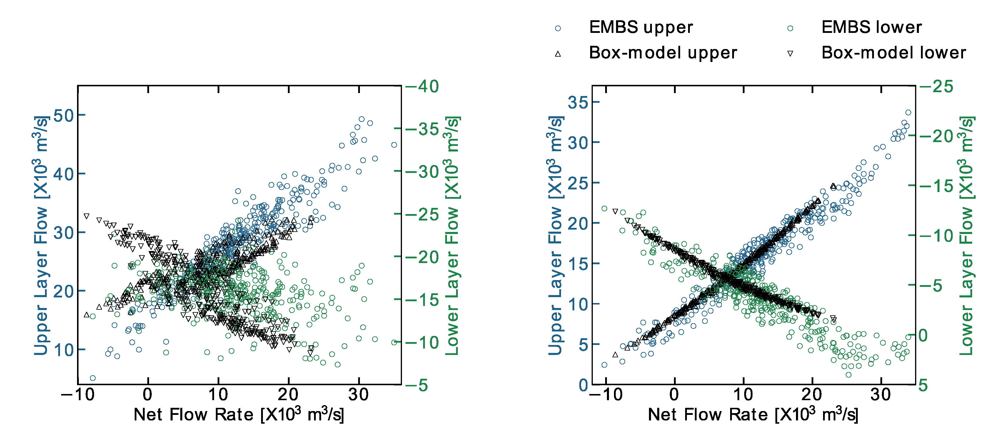
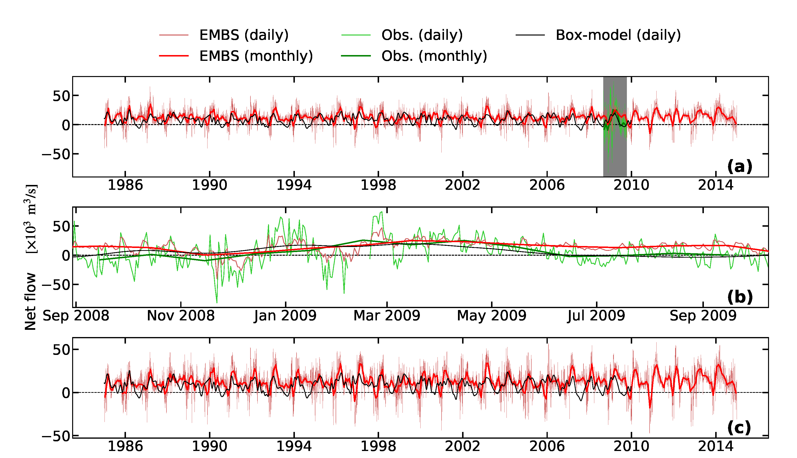
3.3. Water Exchange and Properties at the Straits

The volumetric water exchanges at the two narrow straits of Bosphorus and Dardanelles, as calculated by Maderich et al.’s chain-model, is reproduced by the EMBS simulation (Figure 8). A much higher variability is demonstrated by our simulation, while the upper limit of volume exchange is increased (for the upper as well as the lower layers). Both these changes seem to be improving the calculated flow rates when compared to hydrographic observations at Dardanelles, especially for the upper layer. The spread of both upper and lower layer flows in comparison to the net flow is simulated to be larger in the Dardanelles than in the Bosphorus strait. This difference in the behavior of the two straits is also seen in the chain-model of Maderich, as well as in the observations (see [58]). Time series of the net flow (Figure 9), and the corresponding metrics (Table 4), show that while upper layer flow rates are much higher in our simulation than in the Maderich et al. chain-model (in accordance with observations), the lower layer flow rates are of comparable or slightly lower magnitude, which results in net flow rates being higher overall in EMBS. For the period 2008–2009, this higher upper layer flows as well as the higher variability is an overall improvement when compared to the chain model. Figure 9b shows, as a closeup of Figure 9a, that the variability of the daily net volumetric exchange in our simulation is very similar to that calculated by observations at Dardanelles strait during 2008–2009, while for the chain model the variability of the same quantity is lower, as exhibited by the much smoother time-series.
The simulated seasonal evolution of water characteristics along the Bosphorus–Marmara–Dardanelles system, is compared to known patterns from published observational campaigns [62,63]. The simulated temperature and salinity fields exhibit exceptional agreement with the observed fields, and features like the cold surface waters of Black Sea origin during winter (Figure 10a), the cold tongue between 10–30 m depth during spring (Figure 10b), the relatively warmer deep waters of Aegean Sea origin during summer and autumn (Figure 10c,d) and the overall doming around spots of abrupt changes in bathymetry (the oceanic equivalent of orographic lift), are accurately reproduced. The salinity field remains vertically stratified throughout the year, with low surface values of Black Sea origin and high near-bed values of Aegean origin reflecting the known circulation pattern of water exchange between the two Seas (Figure 11).

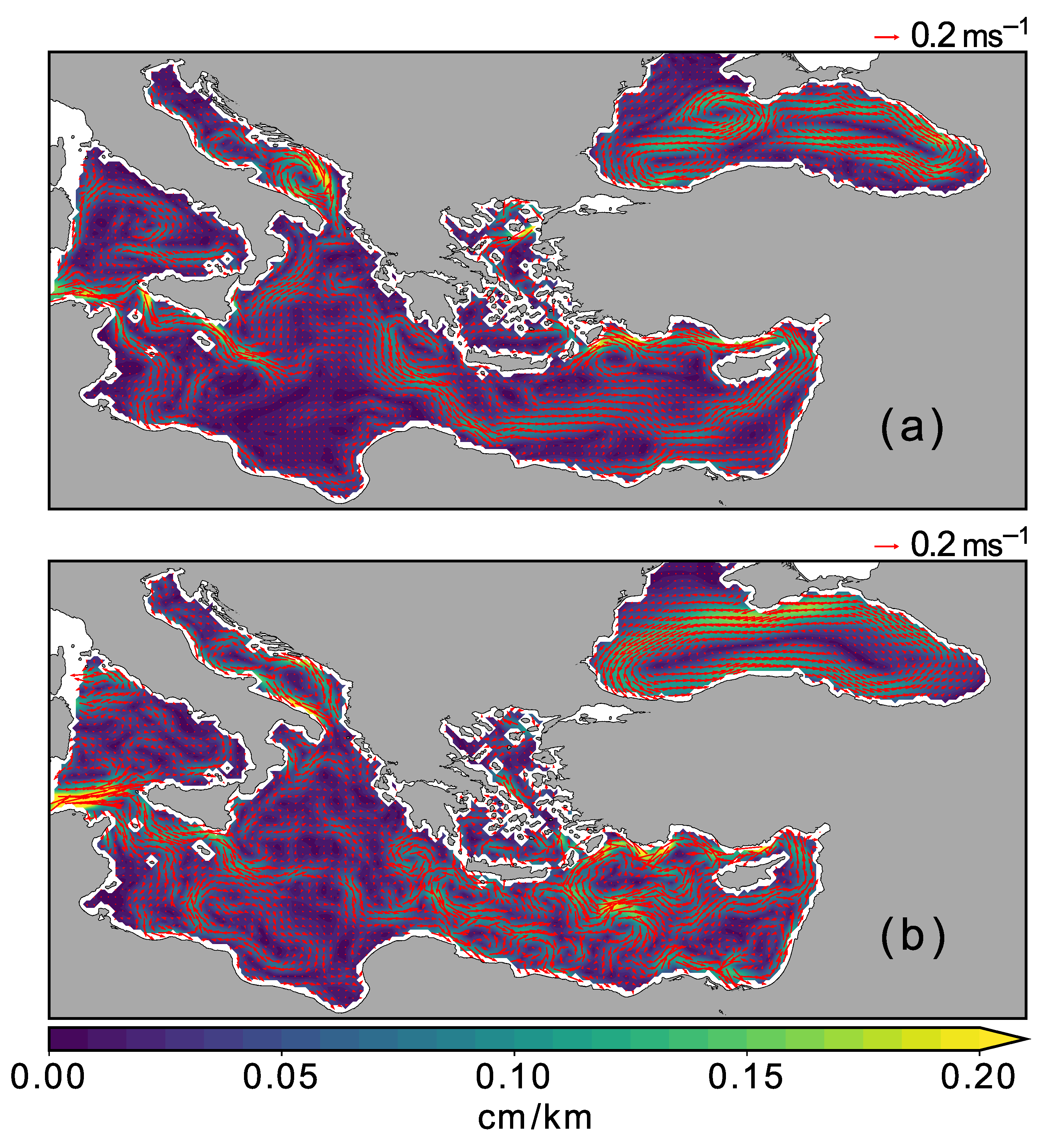
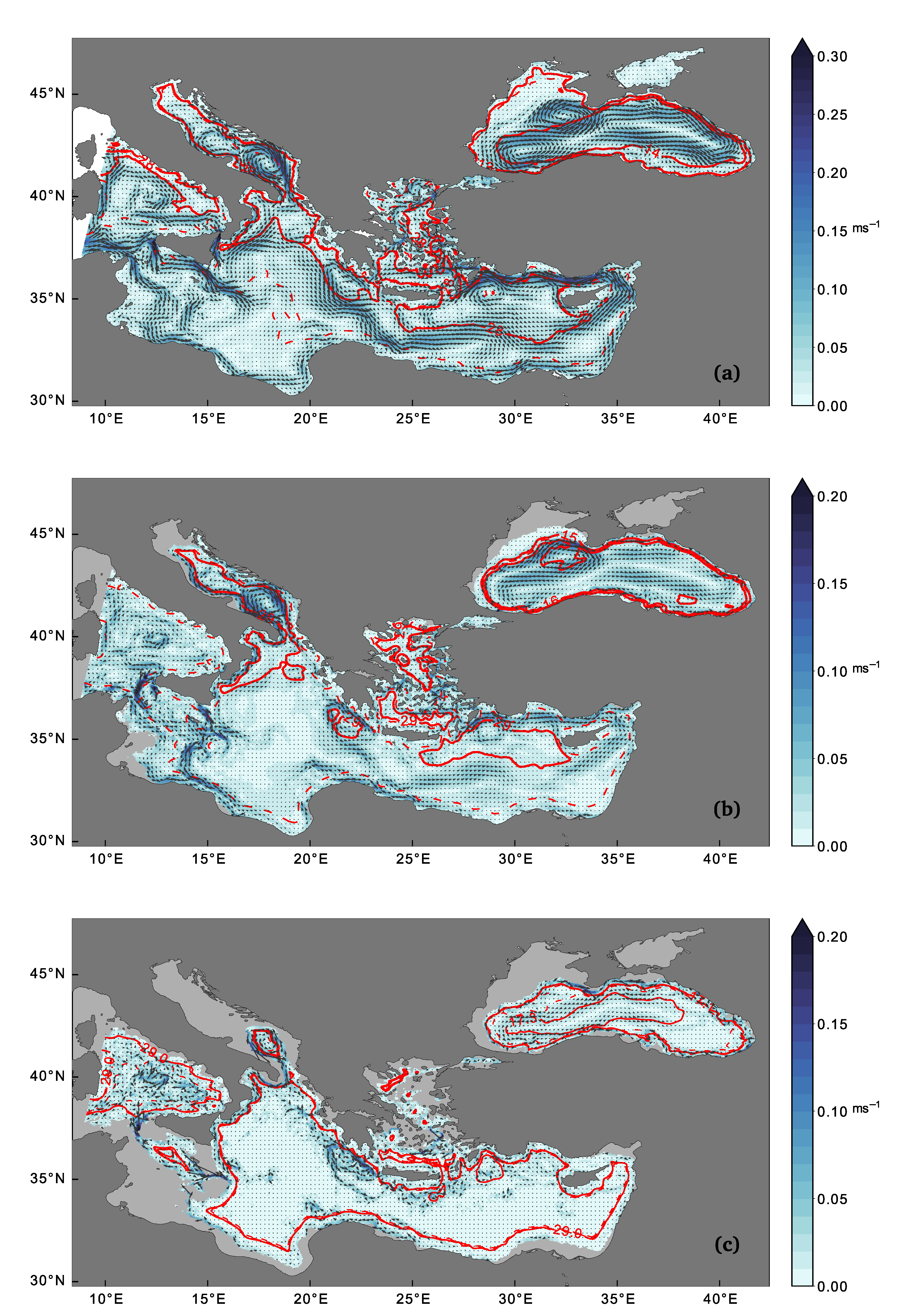
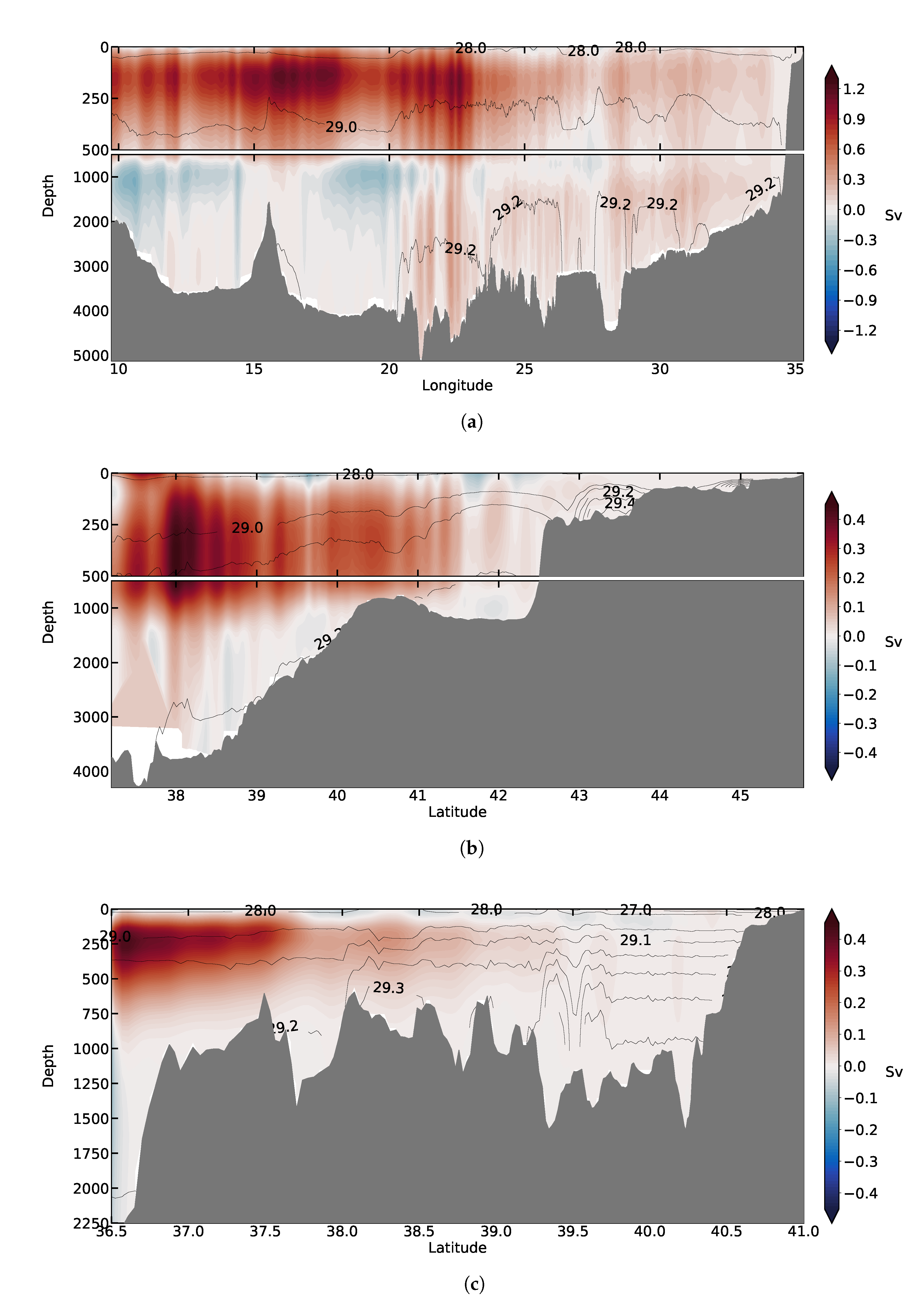
3.4. General Circulation

The simulated mean 1985–2014 current velocity is provided here, averaged over three different vertical layers of the water column (using layer width as the weighing factor), which in combination with meridional and zonal overturning streamfunctions throughout the domain, can provide useful insight regarding the general circulation, as well as the thermohaline circulation of the eastern Mediterranean and Black Sea system, as modeled in the EMBS simulation. The vertical extents of the three layers over which currents have been averaged—namely the surface layer (0–50 m), intermediate layer (50–400 m) and deep layer (400 m–max. depth) shown in Figure 12—were selected using the overturning streamfunctions as a guide for distinguishing between different water mass movements in the vertical (Figure 13).
The zonal overturning streamfunction for the whole eastern-Mediterranean, excluding the Black Sea, is shown in Figure 13a. The eastward moving west-Mediterranean waters of Atlantic origin (reaching 1.2 Sv in the top 120 m) are clearly visible in the clockwise rotating surface layer, which are subject to intense downwelling in the Ionian Sea (between 20°–25° E), stretching down to the bottom ( 22° E). Eastern Mediterranean Deep Waters (EMDW) of relatively high density ( σ θ 29.3 ) are formed near the bottom around that area. The anti-clockwise circulation cell at 1000 m and deeper (blue section roughly between 10 E and 22 E in Figure 13a) is transporting these EMDW further east as can be seen also in the density field at the bottom layers, while transporting Levantine Intermediate Waters (LIW) between 400–1000 m westward over the Sicily strait and into the western-Mediterranean. In the horizontal field, “pools” of increased density extend horizontally from south of the Otranto strait, following the Ionian coast of Greece, to South Crete and then filling the whole southern-Ionian basin (Figure 12). At deeper layers, one can locate the LIW formation site in the north-Levantine between Cyprus and southeast of Crete (Figure 12b), and the EMDW transported eastward around the Rhodes gyre and southeast of Crete (Figure 12c), both of which agree with the known general and thermohaline circulation in the eastern-Mediterranean. In the deep circulation field, increased westward velocities are observed along the bottleneck created by the Sicily straits, transporting LIW to the western Mediterranean (Figure 12b,c). Overall, the highest densities are found in the deep Adriatic (north and south pits 43° N and 42° N in Figure 13b), most of the deep Aegean (Lemnos, Athos, Skyros and Cretan basins, Figure 12c and Figure 13c), and the deep parts of the southern domain (south Ionian, Levantine seas), while the lowest densities are found in the surface waters over the northwest Black Sea shelf.
Following the meridional overturning streamfunction along the north-Ionian and Adriatic Seas (Figure 13b), a northward circulation of 0.1 to 0.4 Sv can be found in the surface to sub-surface layers up to the position of the south and north Adriatic pits ( 42 ° N and 43 ° N respectively), where downward motion is observed and a subsequent doming of the isopycnals, with a returning benthic circulation of high density deep waters ( 29.2 < σ θ < 29.4 ) overflowing back into the south Mediterranean Sea following the bathymetry in a catabatic-like fashion. At the surface and within the first ∼50 m, a southward moving circulation is observed at the northern-most part of the Adriatic, which corresponds to the contribution of riverine waters from Po river forming the west Adriatic current. A very similar picture can be seen in the meridional overturning streamfunction along the Aegean Sea (Figure 13c), with a northward circulation of comparable magnitude (0.1–0.4 Sv) and Levantine origin flowing into the Aegean through the Karpathos strait ( 35 ° N, 27 ° E Figure 12a), flowing up to about 38.5 ° N– 40 ° N, where downward motion contributes to dense water forming at the benthic layers, displaying some of the highest observed water densities of the whole domain ( σ θ 29.5 ). This northward moving surface circulation becomes sub-surface around 38 ° N– 38.5 ° N, under a southward moving surface circulation of North Aegean waters mixed with waters of Black Sea origin (seen as an anti-clockwise surface cell, stretching roughly from 37.5 ° N to 40 ° N—Figure 13c). The benthic southward-moving circulation still exists, but is very reduced when compared to the north-Ionian/Adriatic case, due to the protruding bathymetry of the Aegean, which constrains the southward movement of high density benthic waters; this is consistent with the high densities observed at relatively shallow waters in the north and south Aegean ( σ θ 29.3–29.4 at 500 m depth).

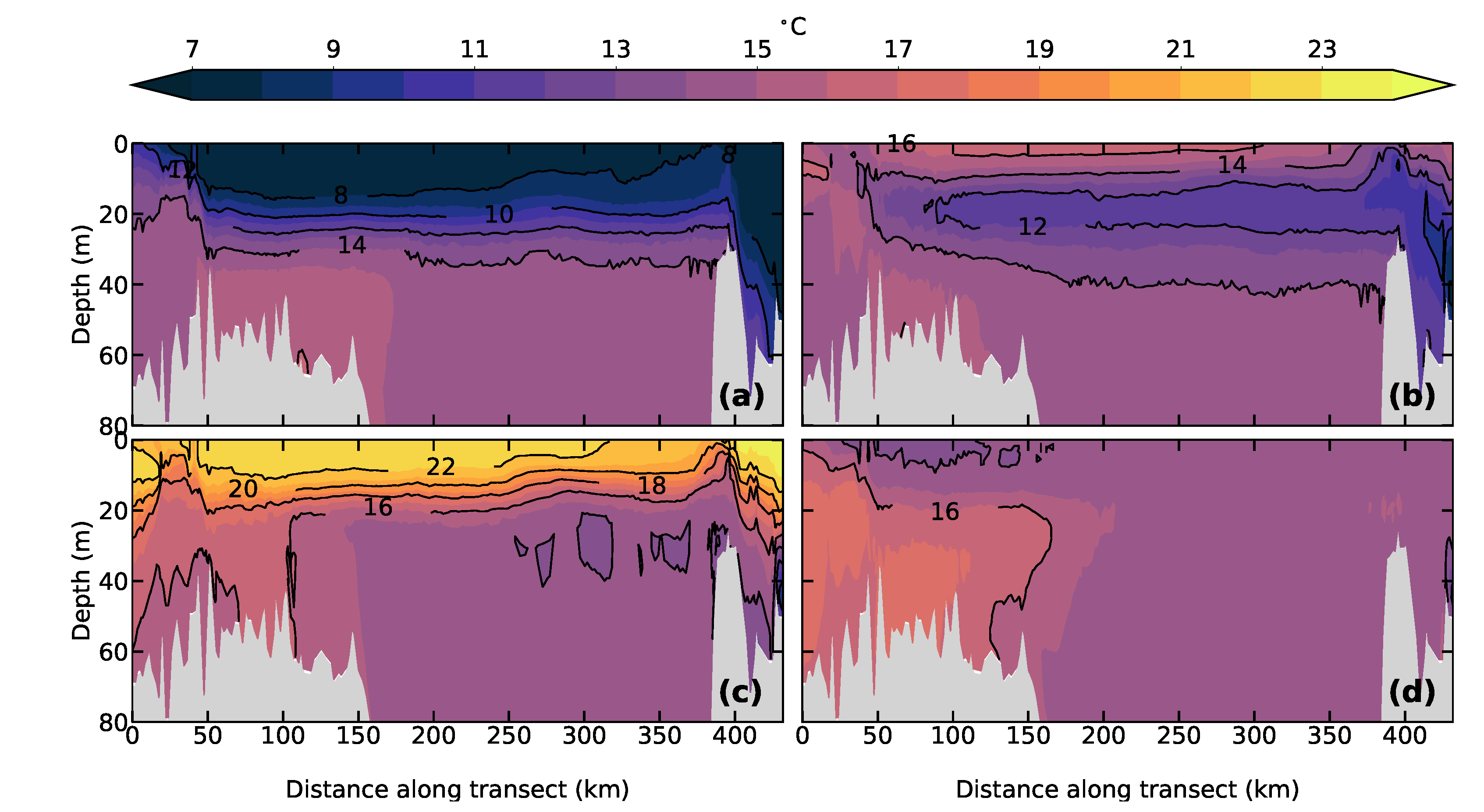
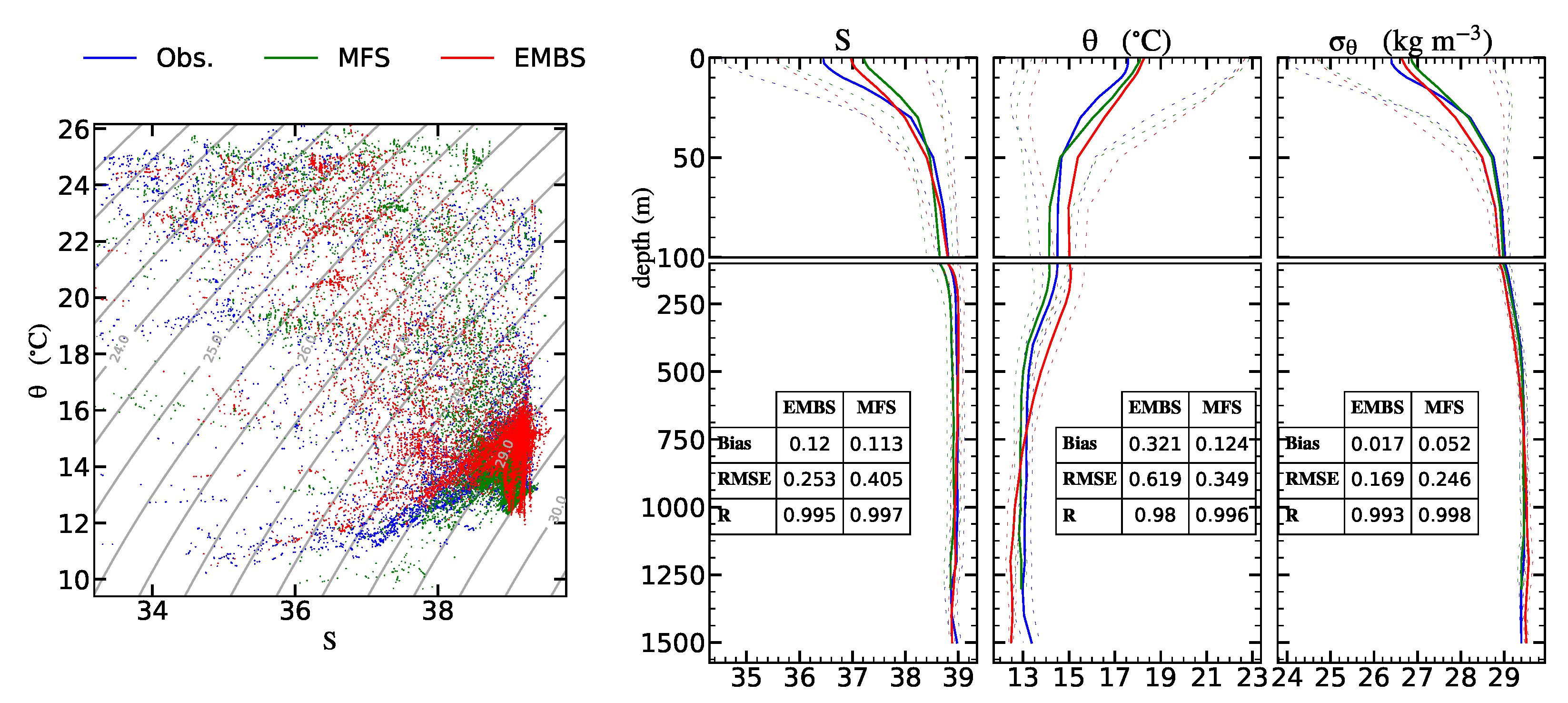
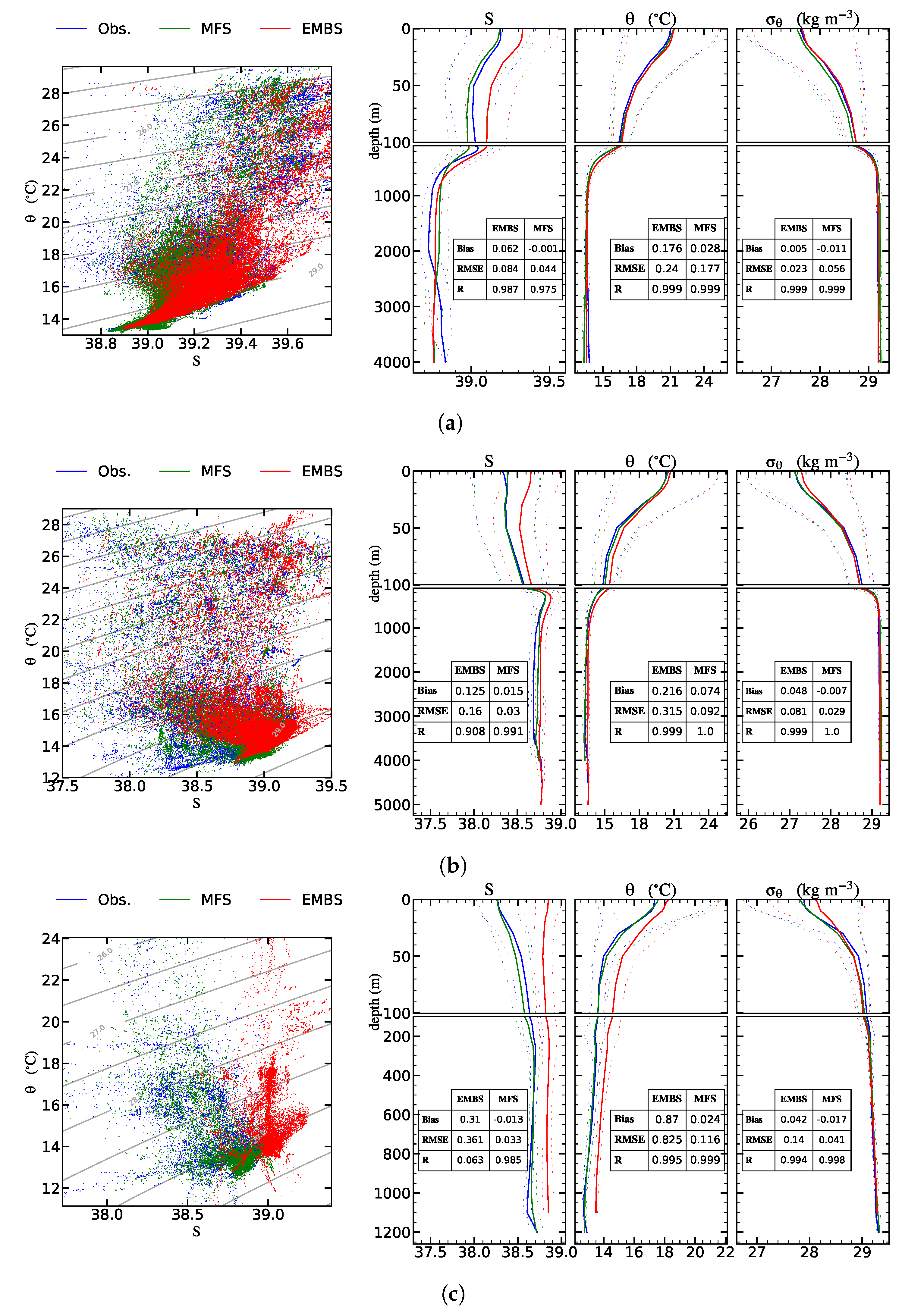
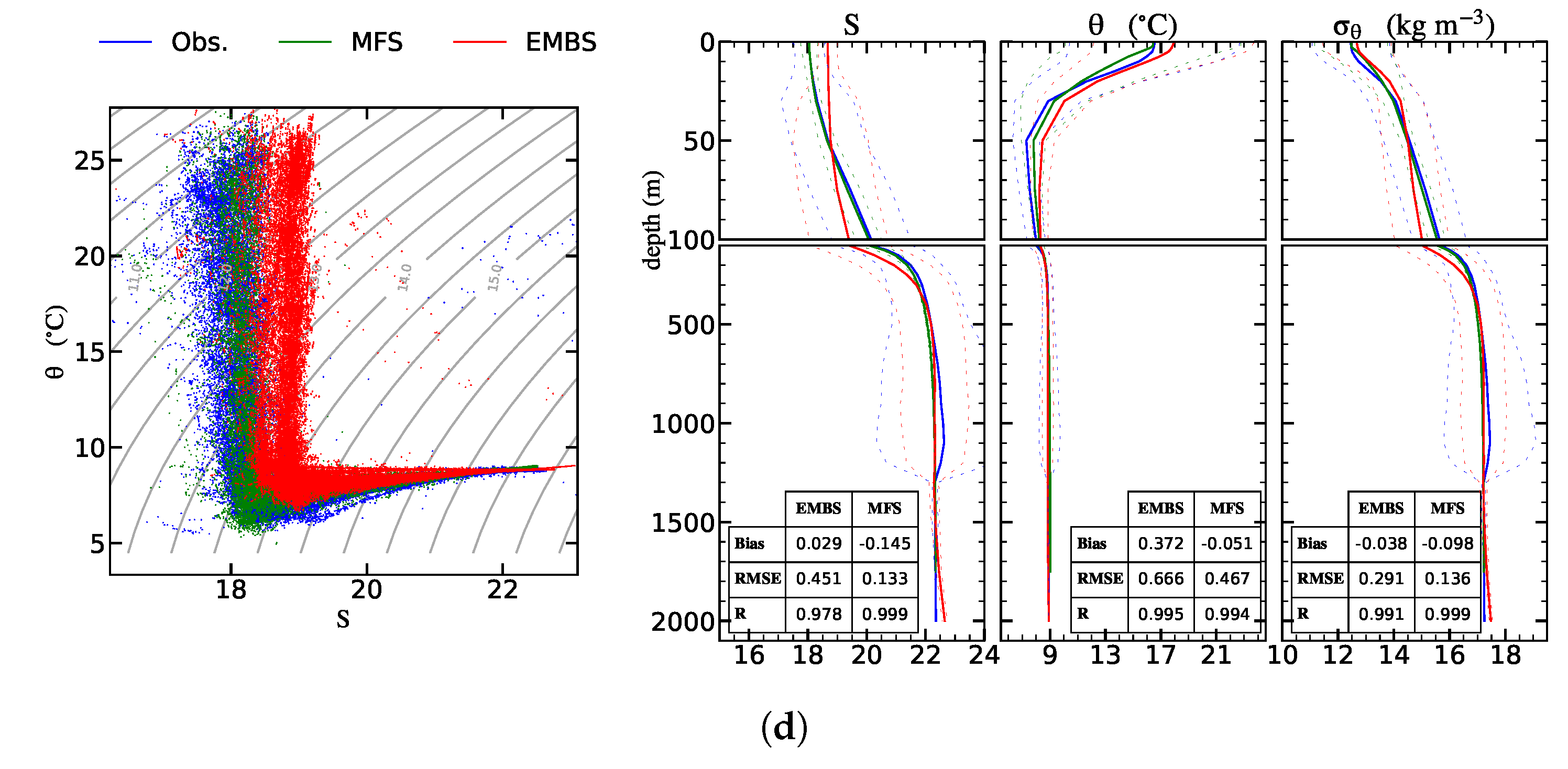
3.5. Column Structure—Profiles

In this final part of the validation process, the vertical structure of the water column is compared to observations and state-of-the-art modeling systems. The comparison shows good agreement with observations, and the variability is reproduced accurately overall. In general, the EMBS simulation overestimates both salinity and temperature systematically over the whole column almost everywhere, nevertheless biases and RMSEs remain fairly low, with a very high correlation coefficient. While the MFS simulation (which makes use of these observations among others, as inputs for its assimilation scheme) reproduces the observations better than the EMBS simulation, the differences are very small. Moreover, in the area of our immediate interest (i.e., the north Aegean Sea), the performance of the EMBS simulation is comparable to the MFS operational forecasting system, especially reproducing vertical structures of the water column and density ranges (Figure 14). As can be seen in the figure, salinity in the north Aegean has a bias of 0.12 and an RMSE of 0.253, and potential temperature has a bias of 0.32 °C and an RMSE of 0.62 °C. Potential density has a bias of 0.017, and an RMSE of 0.169, while the improvement is even higher at the surface layers for all fields. Apart from the mean profiles, points from all the individual profiles in the entire set can be seen in the θ / S diagram, which shows a satisfactory reproduction of the water characteristics of the area in a three-dimensional sense.
A similar profile comparison for different sub-basins can be seen in Figure 15, which demonstrates the spatio-temporal performance of the EMBS simulation (metrics are included as tables within the graphs, with all correlations being statistically significant). The Levantine basin (Figure 15a) is reproduced quite accurately, with surface salinity values being higher due to increased evaporation, and bias and RMSE remaining exceptionally low over all fields. The Ionian Sea (Figure 15b) shows a similar picture; the LIW are clearly visible at ∼100–400 m, and simulation performance remains very high. In the Adriatic, the bias and RMSE especially for potential temperature are among the highest found overall (Figure 15c), the bias at the surface for potential density is around 0.2, but gets much closer to observations when moving downwards into the column, which indicates that the density driven circulation should not be heavily affected. The MFS simulation performs at its best in this sub-basin. In the Black Sea (Figure 15d), again, the performance is acceptable, with most deviations appearing at the surface, especially for the salinity field. It is noteworthy that the EMBS surface salinities at both the Adriatic and the Black Seas exhibit a positive bias, possibly attributed to the omission of minor rivers and thus a potential underestimation of the riverine input in the basins.
Despite the presence of bias in the simulated fields, the θ / S diagram and the vertical profiles of the hydrographic properties reveal a very good reproduction of the distribution of water masses throughout the basin, thus a faithful simulation of the overturning circulation and the production of intermediate and deep waters.

4. Discussion

A novel modeling setup was hereby introduced for the simulation of the interconnected Eastern Mediterranean–Black Sea system (EMBS), in order to produce a tool for improved climatic hindcasts and future projections for the Aegean Sea. The evaluation of the EMBS simulation performance through comparison of the 30-year-long hindcast (1985–2014) to available hydrographic/oceanographic observations and data, exhibits positive results and reveals a satisfactory representation of the physical oceanography of the interconnected Eastern Mediterranean–Black Sea system on climatic timescales, also being among a handful of existing modeling configurations today able to simulate the interacting system. Despite the absence of relaxation and data assimilation schemes, the free-run simulation bias and RMSE are low and consistent for all fields, comparable to operational model results. The structure and intensity of the exchange flows in the straits of Dardanelles and Marmara were reproduced with impressive accuracy, despite the relatively low grid resolution of about 1 km at contraction points and the use of a hydrostatic model. All the goals that were established upon creation of the simulation were achieved (see Section 2.1), with the resulting model proving to be a very capable tool for climate studies in the region. Due to the extended validation of the model presented hereby, a presentation of the interannual variability revealed through the hindcasts is beyond the context of this work. However, as an example of the capacity of the model to reproduce the interannual variability of processes like deep-water formation and mixing during stagnation periods, the interannual variability of density in one of the deep North Aegean sub-basins, northern Skyros basin, as simulated by EMBS is presented in Figure 16. The isopycnal rise during 1987–1994, the subsequent gradual relaxation and deepening during the stagnation period (1994–2000), the following steady-state period until about 2006 and the more recent minor formation episodes are reproduced, as reported by several studies (e.g., [9,10,66]). Furthermore, the interannual variability of the seasonal cycle of the upper-layers is also visible, but a more thorough analysis of the results will be the subject of future work. The validation process and results are discussed in more depth hereafter, providing additional explanation to processes and possible contributing factors to errors or deviations from observations.
Although the representation of simulated surface fields (temperature and surface elevation) as validated against satellite observations/reanalysis is fairly accurate for such an extended free run, there are some discrepancies which can be attributed to either flaws in the model configuration (i.e., grid setup, atmospheric forcing, etc.), or the satellite reanalysis itself. In more detail, the simulation shows some inaccuracies in meso-scale phenomena in the southern part of the domain and especially eddies and gyres south of Crete and in the Levantine basin, specifically: the Pelops Gyre (SW of Peloponnese) appears cyclonic instead of anti-cyclonic, the northern gyre of the Mersa Matruh System (north of Alexandria, Egypt) is properly represented but the southern gyre is missing, the Shikmona Gyre (south of Cyprus), the Ierapetra Gyre (south of Crete) and the Western Cretan Gyre, are all represented, but they appear to be of much lower intensity and/or shifted in position. Spatial variability of the general circulation and sea elevation seems to be reduced when compared to the altimetry (see Section 3.1 and Section 3.2); however, it is similar to that of other modeling systems of comparable configuration like MFS (see [47]), while the gyres mentioned above are much better represented in shorter temporal averages (i.e., daily, monthly, seasonal, etc.—not shown here). The deformation of the grid due to variable resolution leads to a very low ratio of x to y gridbox dimensions in the region (Figure 2), which inserts different scales in the solver and is known by the model developers to be an impediment in smaller scale hydrodynamics. This, together with the relatively higher resolution in the area (5–7 km) can be part of the explanation for the misrepresentation of these few meso-scale phenomena in the southern-most part of the domain by our simulation. However, we cannot rule out the possibility that the discrepancy of the EMBS and AVISO fields could be attributed to the low temporal resolution of the satellite products, in comparison to the near-continuous record of the modeled results. In the latter case, transient mesoscale eddies would be averaged out in a 30-year long record, while averaging over a more discrete data set (as in the case of the satellite record) could result in aliasing causing high wavenumber artifacts. Further investigation of this is not within the context of the present work, but is planned for a subsequent analysis. In other parts of the domain, and especially in coastal regions, land contamination is reported to reduce the accuracy of satellite altimetry [67], while corrections for inverse barometer, tide and high frequency wind effects on the satellite data [68] can lead to reduced accuracy in regions where these corrections are difficult to model. Additionally, inaccuracies in the riverine-discharge dataset can lead to deviations in the temperature and salinity fields, which, keeping in mind the large volumetric flows of rivers involved in this simulation, can be responsible for a considerable fraction of the simulation bias. This is evident when comparing surface fields (e.g., SST in Figure 3) with vertical profiles (e.g., temperature in Figure 15d), where it can be seen that deviations are larger at the surface, but much lower further down the water column, indicating a connection to surface processes (e.g., fresh water input/output through river discharges or through atmospheric forcing precipitation/evaporation). All the above can provide the reasoning behind the larger Bias/RMSE of the simulation in shallow regions, like the north-western plateau in the Black Sea or the northern part of Adriatic Sea (both of which are shallow and recipients of major riverine discharges), the south-east/east coast of the Levantine and other such coastal areas. Nevertheless, on climatic scales the bias, RMSE, and more importantly, the seasonal variability and inter-annual variability of these fields are all very well reproduced. A comparison of the Aegean and Levantine Seas SST with results from comparable models like ALERMO in [69], shows a similar structure of the basin-averaged interannual timeseries and average SSTs, with temperatures being slightly higher overall in our model. This can be partly attributed to the different periods of reference (1960–2000 for the ALERMO run and 1985–2015 for the EMBS). When compared to AVHRR/satellite SSTs, temperatures are slightly overestimated by our simulation and slightly underestimated by ALERMO [11]. Results for the eastern Mediterranean SST from the MED36 simulation in [21], demonstrate an overestimation with respect to the AVHRR timeseries similar to that of EMBS, and a comparable warming trend.
The main reasoning for interconnecting the Black Sea with the Eastern-Mediterranean Sea in a single modeling domain, is the ability to simulate the exchange of water properties between the two domains, enabling one to influence the other as is the case in the physical world. Important efforts have already been established by other studies (i.e., the chain-model of Maderich et al.), towards a physically accurate representation of the long-term climatic water exchange at the Bosphorus–Marmara–Dardanelles straits, in terms of average volumetric flows with part of the respective variability being modeled. Nevertheless, there is plenty of room for improving both the average flow and the full extent of the seasonal/inter-annual variability of the exchange, which is of crucial importance for a physically accurate representation of the interactions taking place between the sub-domains. This has been achieved to a great extent in the EMBS simulation, with large improvements in the average upper layer flow as well as in the overall variability of the flow in both layers (when compared to the chain-model with respect to observations). There has not been such an improvement in the average lower layer flow (with values being comparable to those of the chain-model), and this means that the influence of the Black Sea on the Aegean Sea is going to be more prominent than vise versa (because the lower layer describes the flow from the Aegean to the deep layers of the Black Sea); this is acceptable for the purposes of our study, which focuses on the Aegean/Eastern-Mediterranean Seas. The proper representation of the lower layer flow is hindered in our case, mainly by the hydrostatic approximation of the model in combination with the intensely variable bathymetry at the Bosphorus and especially the Dardanelles straits. However, the improvement in the simulated water characteristics of the Aegean Sea compared to studies that do not incorporate the exchange properly in their resolution is evident in the vertical profiles analysis, proving both the importance and success of such a setup. The analysis of vertical transects along the Bosphorus–Marmara–Dardanelles line shows very good agreement with past observational studies, both for temperature and salinity. The two-layer flow is clearly well-reproduced in the fields. The larger variability of flow partitioning between upper and lower layers in Dardanelles strait, as seen in Figure 8, can be attributed to the physical shape of the two straits and the subsequent differences in hydrodynamic behavior. The Bosphorus strait’s shape is more consistent, with an almost constant width throughout its length, while the Dardanelles strait features a diverse geometry with several contractions and expansions in its width. The consistently narrow, channel-like width of Bosphorus leads to fewer degrees of freedom in a hydrodynamic sense, and a more stable partitioning of the flow between the upper and lower layers compared to Dardanelles. Another factor affecting the variability of partitioning of the flow between upper and lower layers, could be external forcing; the along-strait wind stress on the Dardanelles’ upper layer may display a larger variability compared to Bosphorus, due to the strait’s position as well its direction compared to the locally prevailing winds and/or seasonal systems (i.e., the etesians).
The general circulation follows known patterns as observed by satellite altimetry, and cyclonic and anticyclonic features as well as jets and currents are well reproduced, with the exception being meso-scale phenomena in the southern portion of the domain, as discussed above. In addition, there is a discrepancy in the Black Sea circulation and some patterns are being exaggerated while others depreciated in terms of intensity. The simulated horizontal circulation as discussed above, in combination with the simulated vertical overturning circulation as depicted in zonal and meridional streamfunctions, demonstrate that the thermohaline functioning of the basin is clearly and accurately reproduced, with surface western Mediterranean waters entering the eastern Mediterranean through the Sicily strait, branching in the Ionian to a northward branch towards the Adriatic and an eastward branch towards the Levantine. Intermediate waters are formed in the Levantine (LIW), which then flow towards the western Mediterranean, while Eastern Mediterranean Dense Waters (EMDW) are formed in the south Ionian Sea and disperse towards the deep Levantine. Meridional streamfunctions in the Adriatic and the Aegean highlight the special role and similar functioning of these two basins. It is clear that the diverse bathymetry of the Aegean Sea acts as a hindering factor in the transport of benthic dense water formed in its various deep pits and basins, in contrast with the natural southward slopping of the Adriatic/north-Ionian Seas’ bathymetry, making the transport of dense waters towards the south Ionian much easier in that case. Dense waters formed in the various deep Aegean pits gradually propagate southwards via either turbulent mixing with overlaying layers, or displacement by denser waters. The surface pools of less saline waters, one due to Black Sea inflow and the other due to riverine inflow, are visible in the overturning functioning of the Aegean and Adriatic Seas, respectively. The intensity, shape and volumetric transports of the eastern Mediterranean zonal streamfunction, as well as the Adriatic and Aegean meridional streamfunctions, compare very closely to that presented in [21]. However, the anti-clockwise circulation cell caused by Black Sea water inflow at 40 ° N and 0–250 m depth reaching southward to 38 ° N and 0–100 m depth (Figure 13c), is shallower and not as pronounced in the simulation results of Mavropoulou et al. This can be probably attributed to the better representation of the Black Sea water inflow and its variability in our simulation.
The evaluation of the simulation within the whole water column highlights its exceptional performance for a free-running model. Comparison with in situ profiles as well as operational assimilated model profiles, shows a very accurate representation of both the average profiles as well as their variability, with performance being very close to and even exceeding that of the assimilated model in specific areas. In the north Aegean Sea, there is an evident improvement in the modeling of water characteristics (especially salinity and potential density), which is attributed to the accurate representation of Black Sea water characteristics and inflow. In the Ionian and Levantine basins performance remains very high and close to that of the assimilated simulation (including variability). In the Adriatic and Black Sea, the bias and RMSE for all fields, but especially for salinity, point towards riverine inflow under-representation as a forcing term. It is very probable that the inclusion of only the Po river in the Adriatic leads to an overestimation of both salinity and temperature by the EMBS simulation, a fact nevertheless that translates to a slight overestimation of density only in the first 20–30 m, while being very close to the observations in the rest of the water column. In the Black Sea, similar overestimation is observed while the variability inherent in the observations is reproduced by our model, but not by the assimilated one. In general, all metrics show a very acceptable reproduction of the observed potential density, which is of paramount importance for proper simulation of the density driven flows in the domain.
It is evident from our results and their interpretation, that including the interaction of the Mediterranean with the Black Sea in the simulation configuration, highly improves our capacity to generate long-term simulations of the oceanographic properties and circulation of the domain, especially in the Aegean Sea. The absence of any need for assimilating observational data during the simulation and the minimal drift, if any, that the final product demonstrates, highlight the potential of this modeling setup to be used in hindcast as well as future projection climate studies.

5. Conclusions

Lately, there is an increasing interest on utilizing models as a tool to describe the physical properties of the Mediterranean Sea, either in a purely oceanographic or in a climatic sense. The recent discovery of some physical processes that are unique for the region (e.g., EMT, BIOS, etc.), has supplied the need to study them in retrospect while also projecting possible changes within a changing climate. The majority of modeling studies that investigate the above, use parameterizations to describe the water exchange with the Black Sea, with their results providing evidence that a better description of this interconnection is required for a more realistic representation of the aforementioned processes.
The present study addresses this by creating an ocean simulation tool that realistically replicates the physical oceanography of the Eastern Mediterranean and Black Seas, incorporating their interconnected nature. This tool produced a daily averaged, three-dimensional hindcast dataset for the period (1985–2014), whose performance was hereby exhaustively validated against remote sensing data for the surface fields, modeling and oceanographic survey data for the three-dimensional datasets, observational/modeling data for the volumetric water exchanges at the straits, and qualitative comparison with known features in the region (i.e., vertical overturning circulation, cross-sections of T and S along the straits, general circulation).
The validation process demonstrated that the two-layer exchange flow and its variability at the straits is adequately reproduced, with the lower layer flow being slightly underestimated, while water properties and their spatial and seasonal distribution are well reproduced. Satellite altimetry showed a good performance of the modeled sea surface elevation and its variability, as well as a proper reproduction of the surface general circulation, with a slight underestimation in the intensity and/or spatial variability of some meso-scale gyres. Comparison with satellite datasets showed good performance of the simulation SST and its variability in most regions. Average SSTs were slightly overestimated, the long-term surface warming trend was slightly underestimated, while RMSE was highest in the Black Sea. Validation against observational/modeling vertical profiles showed a good representation of the three-dimensional water properties across the domain, and a comparable performance to modeling systems that make use of data assimilation schemes. Finally, the three-dimensional circulation was examined using different horizontal levels and vertical overturning streamfunctions, matching the otherwise observed/expected behavior for the basin. The validation process has led to an overall positive assessment for the model’s performance (especially considering the absence of relaxation or data assimilation procedures), and the simulation results extend the possibilities for a more comprehensive climate study of the region.
Future work includes taking the hindcast analysis a few steps further, by delving into specific physical processes and/or focusing on sub-domains, while at the same time formulating the conditions for extending this dataset into future projections.

Author Contributions

Conceptualization, E.T. and V.Z.; methodology, S.P., E.T. and V.Z.; software, S.P. and I.G.M.; numerical modeling, S.P.; validation, S.P.; formal analysis, S.P., E.T. and V.Z.; investigation, S.P. and E.T.; data curation, S.P.; writing—original draft preparation, S.P., E.T. and V.Z.; writing—review and editing, S.P., E.T., V.Z. and I.G.M.; supervision, E.T. and V.Z.; project administration, E.T. and V.Z.; funding acquisition, V.Z. All authors have read and agreed to the published version of the manuscript.

Funding

This research received funding from the following two projects: (a) “Infrastructure development for the support of Blue Growth in the North Aegean: Coastal Environmental Observatory AEGIS” (MIS 5021550), funded by the Operational Program “North Aegean 2014–2020” of the European Regional Development Fund and the Region of the North Aegean. (b) European Union’s Horizon 2020 Research and Innovation Program under Grant Agreement No 874990” (EMERGE project). This work reflects only the authors’ view and CINEA is not responsible for any use that may be made of the information it contains.

Institutional Review Board Statement

Not applicable.

Informed Consent Statement

Not applicable.

Data Availability Statement

Not applicable.

Acknowledgments

We would like to thank Nadia Pinardi for the kind provision of all MFS model data used for the construction of oceanic boundary conditions and for the validation of vertical profiles, including periods in which they are not publicly available (i.e., 1985–1986). We also thank Vladimir Maderich for the provision of volumetric flow and hydrographic parameter time-series from his chain model, in the Dardanelles and Bosphorus. The time-series of observed volume fluxes in 2008–2009 from Jarosz et al. were kindly provided by Yiannis Androulidakis. This work was supported by computational time granted from the Greek Research and Technology Network (GRNET) in the National HPC facility—ARIS—under project ID petalas-EMBS2.

Conflicts of Interest

The authors declare no conflict of interest. The funders had no role in the design of the study; in the collection, analyses, or interpretation of data; in the writing of the manuscript; or in the decision to publish the results.

References

  1. Sverdrup, H.; Johnson, M.W.; Fleming, R.H. The Oceans Their Physics, Chemistry, and General Biology; Prentice-Hall: New York, NY, USA, 1942; Available online: https://publishing.cdlib.org/ucpressebooks/view?docId=kt167nb66r (accessed on 1 May 2022).
  2. Pinardi, N.; Özsoy, E.; Latif, M.A.; Moroni, F.; Grandi, A.; Manzella, G.; Strobel, F.D.; Lyubartsev, V. Measuring the Sea: Marsili’s Oceanographic Cruise (1679–80) and the Roots of Oceanography. J. Phys. Oceanogr. 2018, 48, 845–860. [Google Scholar] [CrossRef]
  3. Astraldi, M.; Balopoulos, S.; Candela, J.; Font, J.; Gacic, M.; Gasparini, G.; Manca, B.; Theocharis, A.; Tintoré, J. The role of straits and channels in understanding the characteristics of Mediterranean circulation. Prog. Oceanogr. 1999, 44, 65–108. [Google Scholar] [CrossRef]
  4. Sannino, G.; Herrmann, M.; Carillo, A.; Rupolo, V.; Ruggiero, V.; Artale, V.; Heimbach, P. An eddy-permitting model of the Mediterranean Sea with a two-way grid refinement at the Strait of Gibraltar. Ocean Model. 2009, 30, 56–72. [Google Scholar] [CrossRef]
  5. Dietrich, D.E.; Tseng, Y.H.; Medina, R.; Piacsek, S.A.; Liste, M.; Olabarrieta, M.; Bowman, M.J.; Mehra, A. Mediterranean Overflow Water (MOW) simulation using a coupled multiple-grid Mediterranean Sea/North Atlantic Ocean model. J. Geophys. Res. Ocean. 2008, 113, C07027. [Google Scholar] [CrossRef] [Green Version]
  6. Malanotte-Rizzoli, P.; Manca, B.B.; D’Alcala, M.R.; Theocharis, A.; Brenner, S.; Budillon, G.; Ozsoy, E. The Eastern Mediterranean in the 80s and in the 90s: The big transition in the intermediate and deep circulations. Dyn. Atmos. Ocean. 1999, 29, 365–395. [Google Scholar] [CrossRef]
  7. Roether, W.; Klein, B.; Manca, B.B.; Theocharis, A.; Kioroglou, S. Transient Eastern Mediterranean deep waters in response to the massive dense-water output of the Aegean Sea in the 1990s. Prog. Oceanogr. 2007, 74, 540–571. [Google Scholar] [CrossRef]
  8. Tragou, E.; Petalas, S.; Mamoutos, I. Air–Sea Interaction: Heat and Fresh-Water Fluxes in the Aegean Sea; Springer: Berlin/Heidelberg, Germany, 2022; pp. 1–21. [Google Scholar] [CrossRef]
  9. Zervakis, V.; Georgopoulos, D.; Drakopoulos, P.G. The role of the North Aegean in triggering the recent Eastern Mediterranean climatic changes. J. Geophys. Res. Ocean. 2000, 105, 26103–26116. [Google Scholar] [CrossRef]
  10. Gertman, I.; Pinardi, N.; Popov, Y.; Hecht, A. Aegean Sea Water Masses during the Early Stages of the Eastern Mediterranean Climatic Transient (1988–1990). J. Phys. Oceanogr. 2006, 36, 184–1859. [Google Scholar] [CrossRef]
  11. Vervatis, V.; Skliris, N.; Sofianos, S.S. INTER-annual/decadal variability of the north Aegean Sea hydrodynamics over 1960–2000. Mediterr. Mar. Sci. 2014, 15, 696–705. [Google Scholar] [CrossRef]
  12. Kourafalou, V.H.; Barbopoulos, K. High resolution simulations on the North Aegean Sea seasonal circulation. Ann. Geophys. 2003, 21, 251–265. [Google Scholar] [CrossRef] [Green Version]
  13. Kourafalou, V.; Tsiaras, K. A nested circulation model for the North Aegean Sea. Ocean Sci. 2007, 3, 1–16. [Google Scholar] [CrossRef] [Green Version]
  14. Androulidakis, Y.S.; Krestenitis, Y.N.; Kourafalou, V.H. Connectivity of North Aegean circulation to the Black Sea water budget. Cont. Shelf Res. 2012, 48, 8–26. [Google Scholar] [CrossRef]
  15. Kanarska, Y.; Maderich, V. Modelling of seasonal exchange flows through the Dardanelles Strait. Estuar. Coast. Shelf Sci. 2008, 79, 449–458. [Google Scholar] [CrossRef]
  16. Sannino, G.; Sözer, A.; Özsoy, E. A high-resolution modelling study of the Turkish Straits System. Ocean Dyn. 2017, 67, 397–432. [Google Scholar] [CrossRef]
  17. Sözer, A.; Özsoy, E. Modeling of the Bosphorus exchange flow dynamics. Ocean Dyn. 2017, 67, 321–343. [Google Scholar] [CrossRef]
  18. Aydoğdu, A.; Pinardi, N.; Özsoy, E.; Danabasoglu, G.; Gürses, O.; Karspeck, A. Circulation of the Turkish Straits System under interannual atmospheric forcing. Ocean Sci. 2018, 14, 999–1019. [Google Scholar] [CrossRef] [Green Version]
  19. Ilicak, M.; Federico, I.; Barletta, I.; Mutlu, S.; Karan, H.; Ciliberti, S.A.; Clementi, E.; Coppini, G.; Pinardi, N. Modeling of the Turkish Strait System Using a High Resolution Unstructured Grid Ocean Circulation Model. J. Mar. Sci. Eng. 2021, 9, 769. [Google Scholar] [CrossRef]
  20. Somot, S.; Sevault, F.; Déqué, M.; Crépon, M. 21st century climate change scenario for the Mediterranean using a coupled atmosphere–ocean regional climate model. Glob. Planet. Change 2008, 63, 112–126. [Google Scholar] [CrossRef] [Green Version]
  21. Mavropoulou, A.M.; Vervatis, V.; Sofianos, S. The Mediterranean Sea overturning circulation: A hindcast simulation (1958–2015) with an eddy-resolving (1/36) model. Deep Sea Res. Part I Oceanogr. Res. Pap. 2022, 187, 103846. [Google Scholar] [CrossRef]
  22. Soto-Navarro, J.; Jordá, G.; Amores, A.; Cabos, W.; Somot, S.; Sevault, F.; Macías, D.; Djurdjevic, V.; Sannino, G.; Li, L.; et al. Evolution of Mediterranean Sea water properties under climate change scenarios in the Med-CORDEX ensemble. Clim. Dyn. 2020, 54, 2135–2165. [Google Scholar] [CrossRef] [Green Version]
  23. Sein, D.V.; Mikolajewicz, U.; Gröger, M.; Fast, I.; Cabos, W.; Pinto, J.G.; Hagemann, S.; Semmler, T.; Izquierdo, A.; Jacob, D. Regionally coupled atmosphere-ocean-sea ice-marine biogeochemistry model ROM: 1. Description and validation. J. Adv. Model. Earth Syst. 2015, 7, 268–304. [Google Scholar] [CrossRef]
  24. Ferrarin, C.; Bellafiore, D.; Sannino, G.; Bajo, M.; Umgiesser, G. Tidal dynamics in the inter-connected Mediterranean, Marmara, Black and Azov seas. Prog. Oceanogr. 2018, 161, 102–115. [Google Scholar] [CrossRef]
  25. Napolitano, E.; Iacono, R.; Palma, M.; Sannino, G.; Carillo, A.; Lombardi, E.; Pisacane, G.; Struglia, M.V. MITO: A new operational model for the forecasting of the Mediterranean sea circulation. Front. Energy Res. 2022, 10, 941606. [Google Scholar] [CrossRef]
  26. Sannino, G.; Carillo, A.; Iacono, R.; Napolitano, E.; Palma, M.; Pisacane, G.; Struglia, M. Modelling present and future climate in the Mediterranean Sea: A focus on sea-level change. Clim. Dyn. 2022, 59, 357–391. [Google Scholar] [CrossRef]
  27. Shchepetkin, A.F.; McWilliams, J.C. A method for computing horizontal pressure-gradient force in an oceanic model with a nonaligned vertical coordinate. J. Geophys. Res. Ocean. 2003, 108, 3090. [Google Scholar] [CrossRef] [Green Version]
  28. Shchepetkin, A.F.; McWilliams, J.C. The regional oceanic modeling system (ROMS): A split-explicit, free-surface, topography-following-coordinate oceanic model. Ocean Model. 2005, 9, 347–404. [Google Scholar] [CrossRef]
  29. Hogg, A.M.; Ivey, G.N.; Winters, K.B. Hydraulics and mixing in controlled exchange flows. J. Geophys. Res. Ocean. 2001, 106, 959–972. [Google Scholar] [CrossRef]
  30. Sannino, G.; Carillo, A.; Artale, V. Three-layer view of transports and hydraulics in the Strait of Gibraltar: A three-dimensional model study. J. Geophys. Res. Ocean. 2007, 112, C03010. [Google Scholar] [CrossRef] [Green Version]
  31. Maderich, V.; Konstantinov, S.; Kulik, A.; Oleksiuk, V. Laboratory modelling of the water exchange through the sea straits. OKEANOLOGIYA 1998, 38, 665–672. [Google Scholar]
  32. Weatherall, P.; Marks, K.M.; Jakobsson, M.; Schmitt, T.; Tani, S.; Arndt, J.E.; Rovere, M.; Chayes, D.; Ferrini, V.; Wigley, R. A new digital bathymetric model of the world’s oceans. Earth Space Sci. 2015, 2, 331–345. [Google Scholar] [CrossRef]
  33. Martinho, A.S.; Batteen, M.L. On reducing the slope parameter in terrain-following numerical ocean models. Ocean Model. 2006, 13, 166–175. [Google Scholar] [CrossRef] [Green Version]
  34. Beckmann, A.; Haidvogel, D. Numerical simulation of flow around a tall isolated seamount. Part I: Problem formulation and model accuracy. J. Phys. Oceanogr. 1993, 23, 1736–1753. [Google Scholar] [CrossRef]
  35. Haney, R.L. On the Pressure Gradient Force over Steep Topography in Sigma Coordinate Ocean Models. J. Phys. Oceanogr. 1991, 21, 610–619. [Google Scholar] [CrossRef]
  36. Mellor, G.L.; Yamada, T. Development of a turbulence closure model for geophysical fluid problems. Rev. Geophys. 1982, 20, 851–875. [Google Scholar] [CrossRef] [Green Version]
  37. Galperin, B.; Kantha, L.H.; Hassid, S.; Rosati, A. A Quasi-equilibrium Turbulent Energy Model for Geophysical Flows. J. Atmos. Sci. 1988, 45, 55–62. [Google Scholar] [CrossRef]
  38. Allen, J.S.; Newberger, P.A.; Federiuk, J. Upwelling Circulation on the Oregon Continental Shelf. Part I: Response to Idealized Forcing. J. Phys. Oceanogr. 1995, 25, 1843–1866. [Google Scholar] [CrossRef]
  39. Kantha, L.; Clayson, C. Numerical Models of Oceans and Oceanic Processes. Int. Geophys. Ser. 1994, 66, 940. [Google Scholar]
  40. Smolarkiewicz, P.K.; Margolin, L.G. MPDATA: A Finite-Difference Solver for Geophysical Flows. J. Comput. Phys. 1998, 140, 459–480. [Google Scholar] [CrossRef] [Green Version]
  41. Chapman, D. Numerical Treatment of Cross-Shelf Open Boundaries in a Barotropic Coastal Ocean Model. J. Phys. Oceanogr. 1985, 15, 1060–1075. [Google Scholar] [CrossRef]
  42. Marchesiello, P.; McWilliams, J.C.; Shchepetkin, A. Open boundary conditions for long-term integration of regional oceanic models. Ocean Model. 2001, 3, 1–20. [Google Scholar] [CrossRef]
  43. Flather, R. A tidal model of the northwest European continental shelf. Mem. Soc. R. Sci. Liege 1976, 6, 141–164. [Google Scholar]
  44. Mason, E.; Molemaker, J.; Shchepetkin, A.F.; Colas, F.; McWilliams, J.C.; Sangrà, P. Procedures for offline grid nesting in regional ocean models. Ocean Model. 2010, 35, 1–15. [Google Scholar] [CrossRef]
  45. Fairall, C.W.; Bradley, E.F.; Rogers, D.P.; Edson, J.B.; Young, G.S. Bulk parameterization of air-sea fluxes for Tropical Ocean-Global Atmosphere Coupled-Ocean Atmosphere Response Experiment. J. Geophys. Res. Ocean. 1996, 101, 3747–3764. [Google Scholar] [CrossRef] [Green Version]
  46. Paulson, C.A.; Simpson, J.J. Irradiance Measurements in the Upper Ocean. J. Phys. Oceanogr. 1977, 7, 952–956. [Google Scholar] [CrossRef]
  47. Pinardi, N.; Zavatarelli, M.; Adani, M.; Coppini, G.; Fratianni, C.; Oddo, P.; Simoncelli, S.; Tonani, M.; Lyubartsev, V.; Dobricic, S.; et al. Mediterranean Sea large-scale low-frequency ocean variability and water mass formation rates from 1987 to 2007: A retrospective analysis. Prog. Oceanogr. 2015, 132, 318–332. [Google Scholar] [CrossRef]
  48. Simoncelli, S.; Fratianni, C.; Pinardi, N.; Grandi, A.; Drudi, M.; Oddo, P.; Dobricic, S. Mediterranean Sea Physical Reanalysis (CMEMS MED-Physics). 2019. Available online: https://www.cmcc.it/mediterranean-sea-physical-reanalysis-cmems-med-physics (accessed on 1 February 2020).
  49. Maillard, C.; Balopoulos, E.; The MEDAR Group. Recent advances in oceanographic data management of the Mediterranean and Black Seas: The MEDAR/MEDATLAS 2002 data base. The colour of Ocean Data. In Proceedings of the Internatinal Symposium on Oceanographic Data and Information Management with Special Attention to Biological Data, Brussels, Belgium, 25–27 November 2002. [Google Scholar]
  50. Simoncelli, S.; Schaap, D.; Schlitzer, R. SeaDataNet—Mediterranean Sea—Temperature and Salinity Observation Collection V2. 2015. Available online: https://sextant.ifremer.fr/record/8c3bd19b-9687-429c-a232-48b10478581c/ (accessed on 24 January 2019).
  51. Lindström, G.; Pers, C.; Rosberg, J.; Strömqvist, J.; Arheimer, B. Development and testing of the HYPE (Hydrological Predictions for the Environment) water quality model for different spatial scales. Hydrol. Res. 2010, 41, 295–319. [Google Scholar] [CrossRef]
  52. Venice System, Symposium on the Classification of Brackish Waters, Venice, April 8–14. Arch. Oceanogr. Limnol. 1958, 11, 1–248.
  53. Bellafiore, D.; Ferrarin, C.; Maicu, F.; Manfè, G.; Lorenzetti, G.; Umgiesser, G.; Zaggia, L.; Levinson, A.V. Saltwater Intrusion in a Mediterranean Delta Under a Changing Climate. J. Geophys. Res. Ocean. 2021, 126, e2020JC016437. [Google Scholar] [CrossRef]
  54. Pisano, A.; Buongiorno Nardelli, B.; Tronconi, C.; Santoleri, R. The new Mediterranean optimally interpolated pathfinder AVHRR SST Dataset (1982–2012). Remote Sens. Environ. 2016, 176, 107–116. [Google Scholar] [CrossRef]
  55. Buongiorno Nardelli, B.; Tronconi, C.; Pisano, A.; Santoleri, R. High and Ultra-High resolution processing of satellite Sea Surface Temperature data over Southern European Seas in the framework of MyOcean project. Remote Sens. Environ. 2013, 129, 1–16. [Google Scholar] [CrossRef]
  56. Buongiorno Nardelli, B.; Colella, S.; Santoleri, R.; Guarracino, M.; Kholod, A. A re-analysis of Black Sea surface temperature. J. Mar. Syst. 2010, 79, 50–64. [Google Scholar] [CrossRef]
  57. EU Copernicus Marine Service. Altimeter Satellite Gridded Sea Level Anomalies (SLA) Computed with Respect to a Twenty-Year 2012 Mean. Product SEALEVEL_EUR_PHY_L4_MY_008_068. Available online: https://data.marine.copernicus.eu/product/SEALEVEL_EUR_PHY_L4_MY_008_068/description (accessed on 21 November 2021).
  58. Maderich, V.; Ilyin, Y.; Lemeshko, E. Seasonal and interannual variability of the water exchange in the Turkish Straits System estimated by modelling. Mediterr. Mar. Sci. 2015, 16, 444–459. [Google Scholar] [CrossRef] [Green Version]
  59. Mamoutos, I.; Zervakis, V.; Tragou, E.; Karydis, M.; Frangoulis, C.; Kolovoyiannis, V.; Georgopoulos, D.; Psarra, S. The role of wind-forced coastal upwelling on the thermohaline functioning of the North Aegean Sea. Cont. Shelf Res. 2017, 149, 52–68. [Google Scholar] [CrossRef]
  60. Mamoutos, I.G.; Potiris, E.; Tragou, E.; Zervakis, V.; Petalas, S. A high-resolution numerical model of the North Aegean Sea aimed at climatological studies. J. Mar. Sci. Eng. 2021, 9, 1463. [Google Scholar] [CrossRef]
  61. Jarosz, E.; Teague, W.J.; Book, J.W.; Beşiktepe, S.T. Observed volume fluxes and mixing in the Dardanelles Strait. J. Geophys. Res. Ocean. 2013, 118, 5007–5021. [Google Scholar] [CrossRef] [Green Version]
  62. Beşiktepe, S.T. Density Currents in the Two-Layer Flow: An Example of Dardanelles Outflow. Oceanol. Acta 2003, 26, 243–253. [Google Scholar] [CrossRef] [Green Version]
  63. Beşiktepe, S.T.; Sur, H.I.; Özsoy, E.; Latif, M.A.; Oğuz, T.; Ünlüata, U. The circulation and hydrography of the Marmara Sea. Prog. Oceanogr. 1994, 34, 285–334. [Google Scholar] [CrossRef]
  64. Ciliberti, S.A.; Jansen, E.; Coppini, G.; Peneva, E.; Azevedo, D.; Causio, S.; Stefanizzi, L.; Creti’, S.; Lecci, R.; Lima, L.; et al. The Black Sea Physics Analysis and Forecasting System within the Framework of the Copernicus Marine Service. J. Mar. Sci. Eng. 2022, 10, 48. [Google Scholar] [CrossRef]
  65. Lima, L.; Masina, S.; Ciliberti, S.A.; Peneva, E.L.; Cretí, S.; Stefanizzi, L.; Lecci, R.; Palermo, F.; Coppini, G.; Pinardi, N.; et al. Black Sea Physical Reanalysis (CMEMS BS-Currents). 2020. Available online: https://www.cmcc.it/black-sea-physical-reanalysis-cmems-bs-currents (accessed on 20 July 2021).
  66. Kassis, D.; Korres, G. Recent hydrological status of the Aegean Sea derived from free drifting profilers. Mediterr. Mar. Sci. 2021, 22, 347–361. [Google Scholar] [CrossRef]
  67. Andersen, O.; Scharroo, R. Range and geophysical corrections in coastal regions: And implications for mean sea surface determination. In Coastal Altimetry; Vignudelli, S., Kostianoy, A., Cipollini, P., Benveniste, J., Eds.; Springer: Berlin/Heidelberg, Germany, 2011; pp. 103–146. [Google Scholar]
  68. Ponte, R.M.; Ray, R.D. Atmospheric pressure corrections in geodesy and oceanography: A strategy for handling air tides. Geophys. Res. Lett. 2002, 29, 6-1–6-4. [Google Scholar] [CrossRef]
  69. Vervatis, V.; Sofianos, S.; Skliris, N.; Somot, S.; Lascaratos, A.; Rixen, M. Mechanisms controlling the thermohaline circulation pattern variability in the Aegean–Levantine region. A hindcast simulation (1960–2000) with an eddy resolving model. Deep Sea Res. Part Oceanogr. Res. Pap. 2013, 74, 82–97. [Google Scholar] [CrossRef]
Figure 1. Spatial coverage of the individual sub-basins in the Eastern Mediterranean–Black Sea system, as defined within this study. Azov Sea (AZV), Black Sea (BLK), Marmara Sea (MAR), Aegean Sea (comprised by North Aegean, NAG and South Aegean, SAG), Levantine Sea (LEV), Ionian Sea (ION), Adriatic Sea (ADR), and Tyrrhenian Sea (TYR). Dashed lines indicate the mid-sections upon which potential density is calculated.
Jmse 10 01786 g001
Figure 2. Grid geometry of the simulation. For clarity reasons in this figure, grid lines are drawn at eight times lower resolution (8×) compared to the final product. The equivalent square area grid size of the simulation is shown in color-scale. Final grid is composed of 512 × 1024 horizontal points, with 30 vertical sigma levels.
Jmse 10 01786 g002
Figure 3. Time-averaged SST for the whole simulation period (1985–2014). (a) simulated, (b) bias from satellite (EMBS−AVHRR), (c) RMSE, and (d) Pearson’s R-coefficient for the deseasoned timeseries. All values in degrees Celsius.
Jmse 10 01786 g003
Figure 4. Basin-averaged monthly SST for the whole Eastern Mediterranean–Black Sea system. (a) SST timeseries, (b) deseasoned signal (monthly anomalies), and (c) seasonal SST cycle. All values in degrees Celsius, for satellite reanalysis (black) and EMBS simulation (red).
Jmse 10 01786 g004
Figure 5. Sub-basin temporal-averages of zero-centered ADT for the period 1985–2014, for the EMBS simulation and AVISO satellite reanalysis, with Bias (EMBS−AVISO) and RMSE. All values are in centimeters (cm).
Jmse 10 01786 g005
Figure 6. Horizontal gradient of surface elevation in cm · km−1, and barotropic component of geostrophic currents (red arrows), for the period 1985–2014. (a) EMBS simulation, and (b) AVISO satellite reanalysis.
Jmse 10 01786 g006
Figure 7. At the left column, time-series of spatially-averaged, zero-centered ADT in different sub-basins, for AVISO satellite reanalysis (black) and EMBS simulation (red). At the right column, as above with the seasonal cycle removed (deseasoned). All values in meters (m).
Jmse 10 01786 g007
Figure 8. Volumetric water exchange at Dardanelles (left) and Bosphorus (right), for the two-layers flow. The upper and lower layer flows (y-axes) are compared to the net exchange (x-axes). Results of EMBS simulation are shown with circles, while results from the model of Maderich et al. described in Section 2.3, are shown with triangles, for the whole period in monthly-averaged values.
Jmse 10 01786 g008
Figure 9. Time-series of net volumetric flow: (a) at Dardanelles, (b) at Dardanelles for the period denoted with the gray box, and (c) at Bosphorus. Comparison between the EMBS simulation, the model of Maderich et al., and 1-year-long observations at Dardanelles strait from Jarosz et al. described in Section 2.3, using daily values and monthly averages.
Jmse 10 01786 g009
Figure 10. Seasonally-averaged vertical cross section of potential temperature, along a transect in the Dardanelles–Marmara Sea–Bosphorus line. Horizontal axis spanning from the Dardanelles exit at the Aegean to the Bosphorus exit at the Black Sea. (a) Winter JFM, (b) spring AMJ, (c) summer JAS, and (d) autumn OND.
Jmse 10 01786 g010
Figure 11. Same as in Figure 10, for salinity. (a) Winter JFM, (b) spring AMJ, (c) summer JAS, and (d) autumn OND.
Jmse 10 01786 g011
Figure 12. Currents and potential density for the period 1985–2014, vertically weight-averaged between (a) 0–50 m, (b) 50–400 m and (c) 400 m to maximum depth. Potential density is indicated with red contour lines. In (a,b), increments of 1 kg m−3 are used for solid lines, and 0.5 kg m−3 for dashed lines, while in (c), 0.2 kg m−3 for solid lines, and 0.05 kg m−3 for dashed lines.
Jmse 10 01786 g012
Figure 13. Zonal and meridional overturning streamfunctions for the period 1985–2014. (a) Zonal streamfunction for the Eastern Mediterranean (excluding the Black Sea), (b) Meridional streamfunction for the Adriatic Sea, and (c) Meridional streamfunction for the Aegean Sea. Black contours indicate potential density along the midsection of the domain (see Figure 1).
Jmse 10 01786 g013
Figure 14. North Aegean Sea θ / S diagram containing all profiles (casts) for the period 1985–2014, and average vertical profiles of S , θ and σ θ in the North Aegean Sea. Observations (blue), MFS simulation (green) and EMBS simulation (red) both calculated using profiles at the same place and time as the observations. The range of one standard deviation is shown with dashed lines as a measure of overall variability. Additional metrics for the averaged profiles (Bias, RMSE and R-coefficient) are shown for the two simulations compared to observations, with all correlations being statistically significant (p-value < 0.01).
Jmse 10 01786 g014
Figure 15. Same as Figure 14, for (a) Levantine Sea, (b) Ionian Sea, (c) Adriatic Sea and (d) Black Sea.
Jmse 10 01786 g015aJmse 10 01786 g015b
Figure 16. Hovmöller diagram of simulated potential density with depth for the 30-year period, at Skyros basin, central-north Aegean Sea ( 39 ° N, 25 ° E). Color-scale contours have a spacing of 0.05 kg m 3 , while black contours are shown every 0.5 kg m 3 .
Jmse 10 01786 g016
Table 1. Minimum, maximum and average grid size in km, for each individual basin (side of equivalent square area).
Basin/LocationMin.AverageMax.
North Aegean Sea1.291.852.78
South Aegean Sea2.293.054.15
Ionian Sea2.054.437.34
Levantine Sea2.563.805.61
Black Sea1.492.493.64
Dardanelles/Bosphorus1.211.391.45
Overall1.213.057.34
Table 2. Mean SST from the EMBS-simulation along with metrics of the comparison with satellite reanalysis, for different basins. The Pearson’s R-coeff. is only shown for the deseasoned signal while being statistically significant for all individual grid points in the domain (p-value < 0.01).
BasinSST (°C)Bias (°C)RMSE (°C)Pearson’s R (De-Seasoned)
Aegean Sea19.370.460.8080.824
Adriatic Sea18.620.660.9520.852
Ionian Sea20.860.580.8020.790
Levantine Sea21.550.400.7710.783
Black Sea15.790.761.3100.808
Overall19.610.550.8910.804
Table 3. Metrics of ADT (zero-centered) time-series comparison between EMBS simulation and AVISO satellite reanalysis data, for each sub-basin. Correlations are statistically significant for the whole domain (p-value < 0.01).
BasinBias (m)RMSE (m)Pearson’s R
SeasonalDe-SeasonedSeasonalDe-Seasoned
Aegean Sea0.0120.0530.0350.6920.652
Adriatic Sea0.0120.0490.0310.7020.641
Ionian Sea0.0120.0480.0260.7220.636
Levantine Sea0.0120.0520.0320.6800.616
Black Sea0.0090.0690.0570.4940.590
Overall0.0110.0430.0270.6900.701
Table 4. Average two-layer (upper/lower) and net volumetric flow and standard deviation of flow at the Dardanelles and Bosphorus straits for the EMBS simulation and the box-model of Maderich et al. Comparison for the common period is first shown, while the additional comparison with observations at Dardanelles from Jarosz et al. is included for the period 2008–2009.
(All Flows in [ × 10 3 m 3 s 1 ] )EMBS SimulationBox-ModelObservations
PeriodLocation/LayerMeanStDMeanStDMeanStD
Bosp. Upper15.79.413.94.5
Bosp. Lower4.04.65.62.3
Bosp. Net11.812.18.46.8
1985–2009
Dard. Upper27.613.723.93.6
Dard. Lower15.65.815.74.1
Dard. Net12.011.28.36.8
Dard. Upper29.412.223.23.537.816.4
2008–2009Dard. Lower15.15.316.64.632.813.4
Dard. Net14.410.76.67.75.023.2
Publisher’s Note: MDPI stays neutral with regard to jurisdictional claims in published maps and institutional affiliations.

