Article

INS/GPS Integrated Navigation for Unmanned Ships Based on EEMD Noise Reduction and SSA-ELM

Navigation College, Dalian Maritime University, Linghai Road, Dalian 116026, China
*
Author to whom correspondence should be addressed.
J. Mar. Sci. Eng. 2022, 10(11), 1733; https://doi.org/10.3390/jmse10111733
Submission received: 20 October 2022 / Revised: 7 November 2022 / Accepted: 9 November 2022 / Published: 11 November 2022
(This article belongs to the Section Ocean Engineering)

Abstract

:
The primary problem faced by the integrated navigation system based on the inertial navigation system (INS) and global positioning system (GPS) is providing reliable navigation and positioning solutions during GPS failure. Thus, this study proposes an innovative integrated navigation algorithm to address the limitation of precise positioning when GPS fails. First, for the limitation of noise interference in INS, noise reduction technology based on ensemble empirical mode decomposition (EEMD) is proposed to improve the quality of the INS signal and enhance the noise reduction effect. Second, an INS/GPS integrated framework based on the sparrow search algorithm (SSA) and extreme learning machine (ELM) is proposed. During normal GPS conditions, SSA-ELM is used to develop a high-precision prediction model to estimate differences between INS and GPS. When the GPS signal is interrupted, the difference predicted by SSA-ELM is used as the measurement input and the INS is corrected. To confirm the effectiveness of this method, a real ship experiment is conducted with other commonly used methods. The experimental results demonstrate that the proposed method can improve positioning accuracy and reliability when GPS is interrupted.

1. Introduction

Ship navigation is an important navigation mode to maintain the safe navigation of ships at sea. The emergence and development of computers, sensors, and information technology have led to new ways to enhance ship navigation technology. Currently, the inertial navigation system (INS) and global positioning system (GPS) are the two most popular systems. The INS estimates the carrier’s attitude, position, and velocity information using the inertial measurement unit composed of accelerometers and gyroscopes [1,2,3] and can independently navigate without restrictions. However, cumulative errors accumulate because of the inherent deviation of the gyroscopes and accelerometers and the drift of the velocity and position of the INS over time [4]. GPS can then provide global all-weather continuous navigation information; however, the signal is vulnerable to external interference [5]. Therefore, a single navigation mode cannot meet the requirements of high accuracy and reliability of unmanned ships [6]. To complement each other, both INS and GPS are used for information fusion.
INS/GPS integrated navigation has been popular in dynamic ship navigation [7,8,9,10]. INS/GPS integrated navigation usually adopts a Kalman filter (KF) for the combination [11]. However, because a KF is only applicable to linear systems and requires that the state and measurement equations are linear, it can only be used to estimate the state vector of discrete linear systems. The integrated system exhibits highly nonlinear and non-Gaussian characteristics because of the influence of measurement error on the dynamic navigation of an actual unmanned ship. Thus, it is difficult for the standard KF algorithm to accurately complete data fusion. An extended Kalman filter (EKF) can be effectively applied in INS/GPS integrated navigation and can overcome the limitations of the linear KF [12].
Because the primary inertial measurement units of INS have different noise interferences, reducing the error interference by reducing the noise of the original measurement data is necessary. When the Allan variance analysis method proposed in [13] is used to analyze random errors, a problem of large oscillation occurs under a long correlation time, which affects the denoising effect of inertial measurement units. The wavelet analysis method suggested in [14] establishes a specific random model for denoising errors. The wavelet analysis method then overcomes the Fourier transform’s inability to reflect the instantaneous change in the time domain in the frequency domain [15]. However, the wavelet analysis method has a limitation: the wavelet coefficient is discontinuous at the threshold, and the reconstruction produces turbulence in hard threshold denoising. Soft threshold denoising exhibits excellent continuity, and the wavelet coefficient has a fixed deviation. Furthermore, the signal accuracy is affected after the reconstruction. Therefore, an improved threshold denoising method better than the traditional wavelet hard and soft threshold denoising was proposed in a previous study [15]. Although the improved wavelet threshold has advantageous effects, the coefficient introduced is difficult to determine, and the empirical process is complex [16,17]. To solve the problems associated with the wavelet denoising method, a noise reduction technology based on empirical mode decomposition (EMD) was used to obtain an accurate INS sensor output and improved generalization ability [18]. However, the EMD was prone to modal aliasing. To solve this limitation, an important data preprocessing algorithm based on an EMD interval threshold filter, which is used to remove the noise in inertial sensors and provide accurate information for subsequent modeling, is proposed in this study. Ensemble empirical mode decomposition (EEMD) can effectively solve the modal aliasing phenomenon generated by EMD, and the effect of the time length on the trend is reduced [19].
In recent years, many researchers proposed algorithms to improve the accuracy of INS/GPS integrated navigation when GPS is disturbed. In [20], an integrated positioning technology of an inertial navigator/magnetometer based on a neural network was proposed to solve the long-time interruption of GPS. However, because of the addition of a system, the training time and complexity of the overall system increase. A novel INS error compensation model combining strong tracking Kalman filter (STKF) and a wavelet neural network (WNN) algorithm is proposed in [21]. The authors of [22] presented a dual optimization method composed of the iterative volumetric Kalman filter feedforward neural network (ICKF-FNN) and the radial basis function volumetric Kalman filter (RBF-CKF) to compensate for the position and velocity errors of the integration. Their method improved the stability of the integrated navigation system; however, the network structure was complex. STKF replaced the KF to estimate the INS error. The WNN was used to establish a high-precision model based on STKF when GPS is working normally and to predict INS error during GPS interruption. In addition to the STKF/WNN algorithm, this model can effectively correct independent INS with high accuracy during GPS signal interruption. However, the impact of GPS interruption on the velocity error was not analyzed. In [23], an RBF neural network along with time series analysis was used to predict the measurement update of KF and improve the position, velocity, and attitude accuracy during GPS interruption. However, one limitation of this method is that when the input training samples increase, the structural complexity of the RBF neural network increases and the structure is extremely large, causing an increase in the computational load. In [7], an ELM algorithm for online training of ARIMA models using sliding windows was proposed. This algorithm suffered from not adding generalization performance because of the random generation of ELM initial thresholds and weights. In [24], a double optimization scheme comprising a volumetric Kalman filter (CKF), multilayer perceptron (MLP), and radial basis function (RBF) was proposed. CKF was used to compensate for position and velocity errors during GPS interruption. The double optimization process using different estimators yielded improved error compensation results compared to the single optimization method. However, it had the limitations of multiple hidden layers, large parameters, and challenging training. In [25], KF and the support vector machine (SVM) were used to reliably estimate the vehicle position by limiting the disadvantages of EKF. The sensor used was a GPS enhanced by an inexpensive wireless sensor network. The convolutional neural network short-term memory (CNN-LSTM) model was proposed in [26]. A convolutional neural network was used to quickly extract input features, and the LSTM network was used to output pseudo GPS signals as compensation objects to improve the performance of the integrated navigation system. When these neural network algorithms are applied to the INS/GPS integrated navigation system, the aim is to train the neural network with INS input data using the KF as training samples. When the GPS has a signal, INS/GPS integrated navigation uses a KF to correct INS position errors. During GPS interruption, the INS error is corrected using trained neural network output. However, in INS/GPS integrated navigation, the high-level random noise, uncertainty in INS sensors, and the complex model of real noise data form an important problem. In this uncertainty-oriented environment, intelligent structures with additional degrees of freedom can handle and model the high uncertainty in INS sensors; efficient noise reduction technology, the predecessor of intelligent structures, is an effective solution [18].
An unmanned ship induces significant estimation errors in the positioning information in a dynamic environment. Thus, to obtain reliable and accurate positioning information during GPS interruption, a new integrated navigation algorithm is proposed. First, a noise reduction method based on EEMD is proposed to reduce the original INS measurement noise, enhancing the input accuracy of training. There is considerable noise interference in the inertial measurement unit, and EMD is prone to modal aliasing [27]. EEMD first preprocesses the signal and then performs EMD. Therefore, EEMD can inherit all the advantages of the EMD algorithm and effectively limit the problem of modal aliasing [28], thus providing accurate information for subsequent INS/GPS data fusion and model training. Second, as the initial weights and thresholds of the extreme learning machine (ELM) are randomly generated, a sparrow search algorithm (SSA) is proposed to optimize the initial weights and thresholds in the neural network, improve the ELM prediction performance, and improve the prediction performance when GPS is interrupted. Finally, the high accuracy and reliability of the algorithm are confirmed by the real ship test.
The remainder of this paper is structured as follows. Section 2 details the basic principle of INS/GPS integrated navigation. Section 3 introduces the methods proposed in this study, including the noise reduction method based on EEMD to process the original inertial measurement unit (IMU) and the INS/GPS fusion model based on SSA-ELM during GPS interruption. Section 4 introduces the experiment and discusses and analyzes the experimental results to confirm the proposed hybrid method. Section 5 presents the conclusions.

2. INS/GPS Integrated Navigation System

2.1. INS System Error Equation

The constructed INS error equation uses the local geographic coordinate system as the navigation coordinate system (n system). The local geographical coordinate system comprises the east-north-up (ENU), carrier (b system), earth (e system), and inertial (i system) coordinate systems. INS obtains the initial velocity, position, and attitude through initial alignment and can predict the ship’s real-time position, velocity, and attitude through integral measurement. The INS solution diagram is shown in Figure 1. The INS navigation equation primarily includes the attitude, velocity, and position error equations:
  • Attitude error equation:
    φ ˙ n = δ ω i e n + δ ω e n n ω i e n + ω e n n × φ n C b n δ ω i b b  
    where the superscript n indicates the navigation coordinate system (n system), φ n = φ e   φ n   φ u is the attitude error matrix, ω i e n = 0   ω i e   c o s L   ω i e   s i n L is the angular rate vector of the earth relative to the system, ω e n n is the angular velocity vector from the n system to the earth and can be expressed as (2), C b n is the transformation matrix from the b to n system, and ω i b b is the random drift of the gyroscope under the b system.
    ω e n n = V n R n + h V e R m + h V e t a n L R m + h T  
  • Velocity error equation:
    δ V ˙ n = f n × φ n + δ V n × 2 ω i e n + ω e n n + V n × 2 δ ω i e n + δ ω e n n + δ g + C b n δ f b  
    where, in n system, f n is the specific force vector measured by the accelerometer, δ g is the gravity error, C b n is the conversion matrix from the b to n system, and in the n-coordinate system, δ f b is the deviation of the accelerometer.
  • INS position error equation:
    δ L ˙ δ λ ˙ δ h ˙ = 0 1 R n + h 0 s e c L R m + h 0 0 0 0 1 δ V e δ V n δ V u + 0 V n ( R n + h ) 2 V e s e c L t a n L R m + h V e s e c L ( R m + h ) 2   0 0 δ L δ h
    where the longitude, latitude, and earth height of the carrier position are φ , λ , and h respectively; δ L ˙ , δ λ ˙ , and δ h ˙ represent their corresponding errors; V e , V n , and V u . V u are the velocities of the carrier in the three directions of ENU in the n system; δ V e , δ V n , and δ V u are their corresponding errors; and R n and R m are the radii of curvature on the meridian and the primordial perpendicular, respectively.

2.2. Extended Kalman Filter

Because of the inertial measurement noise in the IMU, the independent INS rapidly diverges. To suppress the divergence of the independent INS and improve the INS equipment performance, the loose INS/GPS integrated navigation system is used in this paper, and the INS and GPS are integrated using EKF. The loosely integrated navigation system uses the position and velocity errors of INS and GPS to establish a 15-dimensional state vector:
X = φ E , φ N , φ U , δ v E , δ v N , δ v U , δ L , δ λ , δ h , ε x , ε y , ε z , σ x , σ y , σ z T
where the attitude angle error is φ E , φ N , φ U ; the east, north and up velocity errors are δ v E , δ v N , δ v U ; the longitude, latitude, and attitude position errors are δ L , δ λ , δ h ; and the gyro measurement error and accelerometer zero bias are ε x , ε y , ε z , σ x , σ y , σ z .
The state and measurement equations of the system are expressed as follows:
X ˙ = A × X + B × W Z = H × X + V = P I N S V I N S P G P S V G P S
where the state vector and its differential are X and X ˙ , respectively, and the 15 × 15 state transition matrix is A, which can be calculated based on the velocity, position, and attitude error equations of the INS. The system noise matrix and the system noise vector are B, W; the measurement matrix and measurement noise are H, V. The INS and GPS position observations are PINS, VINS. The INS and GPS velocity observations are PINS, VINS.. The corresponding observation matrix, 03, is shown in (7), which characterizes the 3 × 3 zero matrix, and the 3 × 3 identity matrix is I3.
H = 0 3   0 3   I 3   0 3   0 3 0 3   I 3   0 3   0 3   0 3
(6) is discretized based on the INS error model, as shown in (8):
X k = φ X k 1 , W k 1 Z k = h X k , V k  
where the nonlinear function of the state process is φ , the state vector is X k , the state vector at time k 1 is X k 1 , the process noise at time k 1 is W k 1 , the measurement vector is Z k , the nonlinear function of the measurement process, and the process noise is V k .
1.
Time update:
X ^ k ¯ = φ X ^ k 1 , 0 P k ¯ = A P k 1 A T + W Q W T
where P k stands for the prior estimation of the state at time k , X ^ k 1 stands for the posterior estimation at time k 1 , P k ¯ stands for the covariance matrix of the prior error, A stands for the state transition matrix from k 1 to k, R , W stands for the system noise distribution matrix, and Q stands for the process noise covariance matrix.
2.
Measurement update:
K k = P k ¯ H T H P k ¯ H T + V R V T 1 X ^ k = X ^ k ¯ + K k Z k h X ^ k ¯ , 0 P k = I K k H P k ¯
where K k is the K F gain, H is the measurement matrix, V is the measurement noise distribution matrix, R is the measurement noise covariance matrix, X ^ k is the state update, and P k is the covariance update.

2.3. Proposed INS/GPS Integrated Navigation System Framework

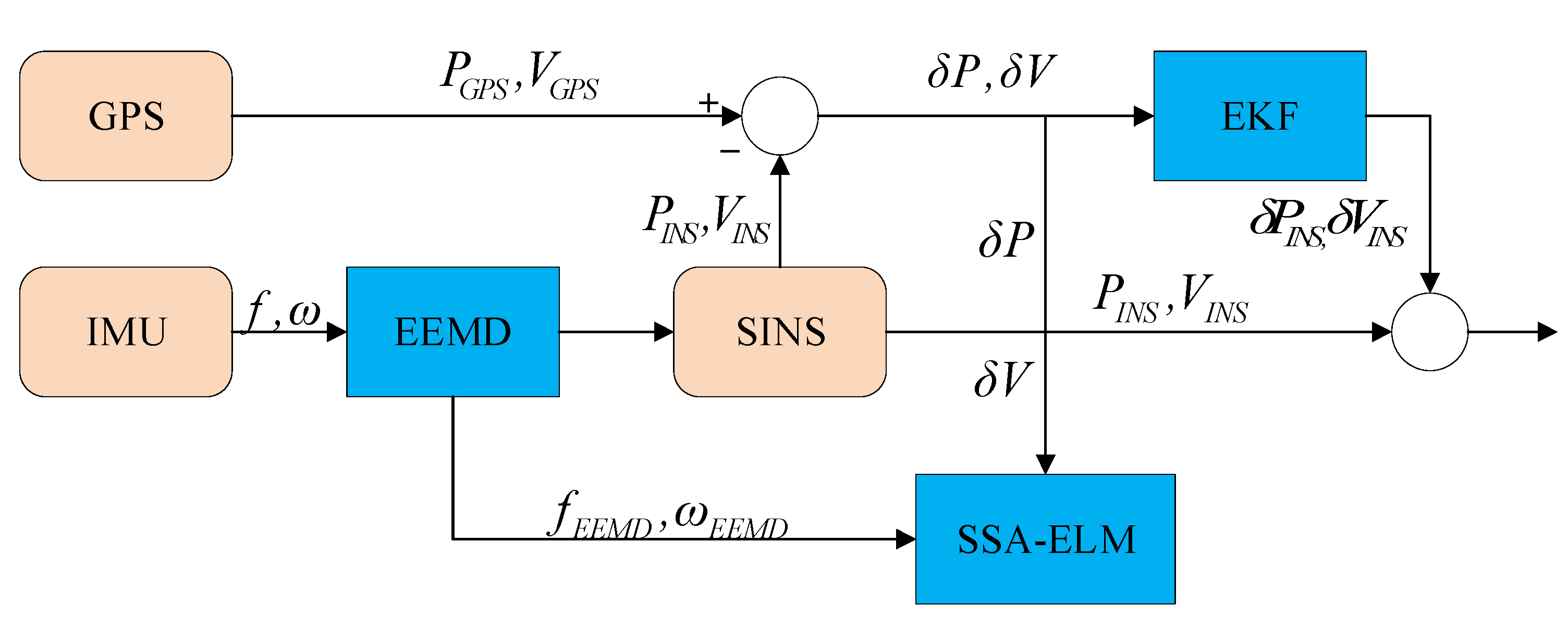
The proposed INS/GPS integrated navigation system, which includes the training and prediction modes, is shown in Figure 2 and Figure 3.
Figure 2 shows that the INS error accumulation is corrected when the GPS is available by fusing the GPS output information with INS. In the INS/GPS integrated navigation system, the three-axis acceleration ( f x , f y , f z ) and angular velocity ( ω x , ω y , ω z ) output of the IMU are obtained via the mechanization equation to obtain the position, velocity, and attitude information of the INS. There is noise interference in the IMU inertial measurement unit. In Figure 2, EEMD is used to denoise the three-axis acceleration and angular velocity of the IMU. The denoised acceleration and angular velocity are input into the INS mechanization equation to obtain accurate velocity, position, and attitude information. Then, the denoised acceleration and angular velocity are input into the neural network model, and the output is the observation value output by the system. The position and velocity difference of INS/GPS is considered as the measured value of EKF, and then the neural network model is trained.
Figure 3 shows that during GPS interruption, the INS/GPS integrated navigation system is in prediction mode and the INS error is predicted through the trained neural network model. In Figure 3, EEMD is used to denoise IMU and input the denoised information into the INS mechanization equation to obtain an accurate position, velocity, and attitude information. During GPS interruption, IMU acceleration and angular velocity information are input into the neural network model and the observation value of the integrated navigation system is predicted. The output result of SSA-ELM is the prediction result, which is used as the measurement input in the EKF update process to further improve the navigation accuracy of the integrated navigation system during GPS interruption. The predicted INS and GPS position and velocity errors are input in the EKF to estimate the INS position and velocity error and correct the INS output.

3. Proposed Method

3.1. EEMD Denoising

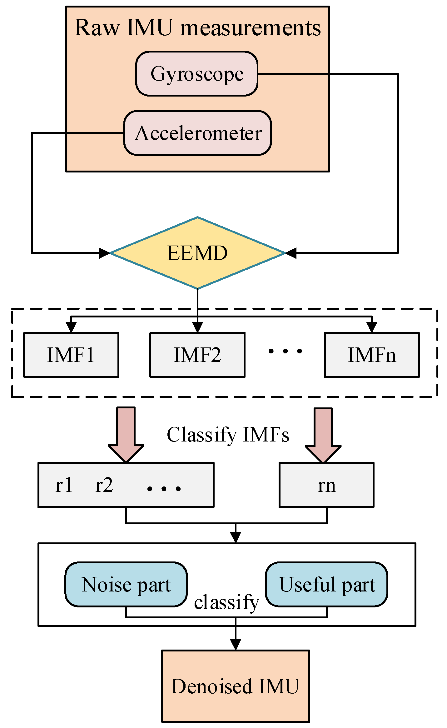
The EEMD method was proposed in [29] to solve the limitation of modal aliasing, which may occur during EMD decomposition. EEMD can decompose nonlinear signals into a series of intrinsic mode functions (IMFs), prevent modal aliasing and improve the analysis effect of signals [30]. EMD is popular in signal denoising, but modal aliasing is a limitation in EMD decomposition and affects the denoising effect. To solve this limitation, the EEMD method is suggested to improve modal aliasing. The EEMD decomposition diagram is shown in Figure 4, and the decomposition steps of EEMD are as follows:
1.
The overall average number M and the amplitude coefficient k of white noise are set. In this paper, M is 100, and k is 0.2 times the signal standard deviation.
2.
A random Gaussian white noise sequence n i ( t ) is added to the original signal x ( t ) to obtain a new signal x i ( t ) .
x i ( t ) = x ( t ) + n i ( t ) , i = 1 , 2 , , M .
3.
EMD decomposition is performed on the new signal x i ( t ) to obtain n IMF components c i , j ( t ) and a residual component r n , j ( t ) , j = 1 , 2 , , n .
4.
Steps 2 and 3 are repeated for M times of EMD decomposition, and the means of all IMF and participating components are calculated to obtain the EEMD decomposition result.
c j ( t ) = 1 M i = 1 M c i , j ( t )
r j ( t ) = 1 M i = 1 M r n , j ( t )
The original signal is decomposed into a limited number of IMF components through EEMD, the sequence from high frequency to low frequency is the arrangement of IMF components after decomposition, and the correlation between the original signal and each IMF component is calculated as per the correlation coefficient r . The calculation formula of r is shown in (14). The IMF component is divided into noise and useful signals as per r ; the noise signal is removed, and the useful signal is reconstructed to obtain the denoised signal.
r x y i = C o v x , y i V a r x V a r y i
where x is the original signal in the IMU, y i is the i-th IMF component, and r x y i is the correlation coefficient of x and y i .
Overall, the degree of correlation is determined according to Table 1. If the r is above 0.5, it is a noise signal; otherwise, it is an original signal. The original signal is reconstructed to form a denoised signal. Furthermore, the effects of EMD and EEMD are compared using the RMSE and SNR of (15) and (16).
R M S E = 1 N i = 1 N y i x 2
where N is the number of each IMF component, y i is each IMF component, and x is the original signal.
P S N R = 10 log 10 ( 2 n 1 2 M S E )
where MSE is the mean square error of the denoised and reference images.

3.2. SSA-ELM Model

The SSA can be used to solve the limitation of falling into an optimal local solution caused by random initialization of weights and thresholds. Furthermore, the initial weights and thresholds of ELM are optimized through SSA, and the fitness function is the mean square error (MSE) after training. Each individual in the population represents the initial weight and threshold of the ELM. When the MSE is reduced, the coincidence between the predicted and original data increases. The final optimized output is the optimal initial weight and threshold. Subsequently, the dataset is tested using the network trained by the optimal initial weight threshold.

3.2.1. Sparrow Search Algorithm

The inspiration of SSA comes from the feeding and anti-catching behavior of sparrows, and it is a new swarm intelligence optimization algorithm [31]. It has strong global optimization ability, does not rely on gradient information, and has good parallelism and fast convergence speed.
The initialization of the sparrow population is shown as follows:
X = x 1 1 x 1 2 x 1 n x 2 1 x 2 2 x 2 n x n 1 x n 2 x n d
The general sparrow fitness representation form is given as follows:
F x = f ( [ x 1 1   x 1 2     x 1 n ] ) f ( [ x 2 1   x 2 2     x 2 n ] ) f ( [ x n 1   x n 2     x n d ] )
During foraging, the producer’s position is constantly moving, and when he meets a predator, the moving rules will change:
X i , j t + 1 = X i , j e x p ( i α · i t e r max ) , i f   R 2 < S T X i , j + Q L , i f   R 2 S T
The updated mode of participants is given as follows:
X i , j t + 1 = Q e x p ( X w o r s t X i . j t i 2 ) , i f   i > n / 2 X P t + 1 + X i , j X P t + 1 A + L , o t h e r w i s e
The updated location of the watchman is given as follows:
X i , j t + 1 = X b e s t t + β X i , j t X b e s t t , i f   f i > f g X i , j t + K ( X i , j t X w o r s t t ( f i f w ) + e ) , i f   f i = f g
The main steps of the sparrow algorithm are as follows:
1.
Initialize the population. The total population of sparrows is expressed as y Set the number of sparrows aware of danger, the number of discoverers, the maximum number of iterations i t e r m a x and the alarm threshold R 2 .
2.
Select the mean square error (MSE) as the fitness function to calculate the fitness value of each sparrow, then identify the best and worst fitness values, which are respectively f g and f w .
3.
Use (19) and (20) to calculate the new position of the discoverer, the forager, and the sparrow aware of the danger. If the fitness value of the new position is better than that of the previous position, the position will be updated.
4.
Iterate, repeat step 3, and constantly update the position of the best sparrow. When the number of iterations increases i t e r m a x , the iteration should be stopped. The optimal solution is the sparrow of the lowest fitness value in all iterations.

3.2.2. Extreme Learning Machine

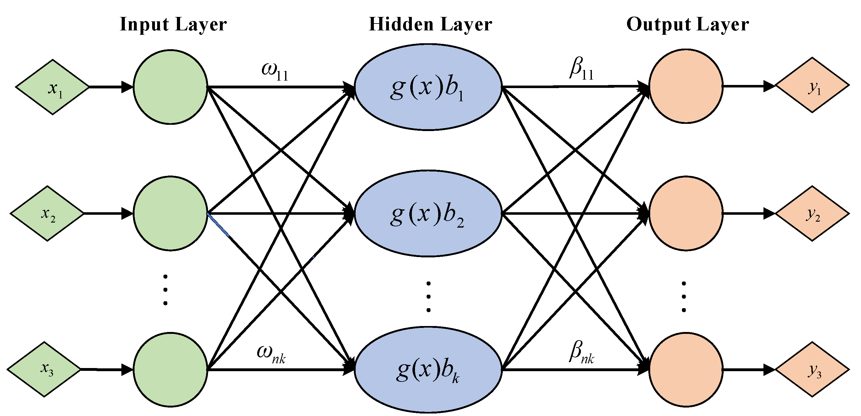
In [32], ELM for solving single hidden layer feedforward neural network is proposed, which mainly uses the generalized inverse theory of the matrix. Compared with the traditional neural network algorithm, the ELM algorithm has the advantages of fewer parameter settings, less computation, faster learning speed, better generalization ability, and higher function approximation ability. The ELM model diagram is shown in Figure 5.
In Figure 5, x 1 ~ x n is a node of an input neuron, ω 11 ~ ω n k is the weight between the input and hidden layers, g ( x ) is the activation function, b 1 ~ b k is the threshold of the hidden layer node, β 11 ~ β n k is the weight between the hidden and output layers, and y 1 ~ y n is the output for the model. Suppose that there are N training samples x i , t i i = 1 N , x i = x i 1 , x i 2 , x i 3 , , x i n T R n is the n-dimensional input data of the training set, and t i = t i 1 , t i 2 , t i 3 , , t i n T R m is the m-dimensional ideal output value of the training set. For K hidden layer nodes, the ELM network model’s expression of the activation function g i x i is as follows:
y j = i = 1 K β i g i ω i x j + b i , j = 1 , 2 , K
Here, ω i represents the input weight vector connected between the input and i t h hidden layer nodes, β i represents an output weight vector connected between the i t h hidden and output layer nodes, b i represents the threshold of the second hidden layer node, y j represents the actual output of the network model, and g i ω i x j + b i represents the activation function.
When the single feed neural network with K hidden layers may approach any N training samples of zero error, it is shown as follows:
i = 1 N y i t i = 0
At this time, the following is obtained:
t j = i = 1 K β i g i ω i x j + b i , j = 1 , 2 , , N
The N equations in the formula can be abbreviated as follows:
H β = T
wherein
H = g 1 ω 1 x 1 + b 1 g i ω K x 1 + b K g i ω 1 x N + b 1     g i ω K x N + b K N × K
where H represents the output matrix of the hidden layer, and T represents the ideal output vector.
Here, it is necessary to find the least square solution of the linear system H β = T . According to the generalized inverse theory of the matrix, the solution is as follows:
β ^ = H + T
Here, H + represents the augmented inverse matrix of the H matrix. The learning speed of ELM is very fast. Since ω and b are randomly generated by the network before training, we only need to determine the number of nodes in the hidden layer and the corresponding activation function g ( x ) to calculate β . The best solution only needs to be run once during the training process.

3.2.3. SSA-ELM Model

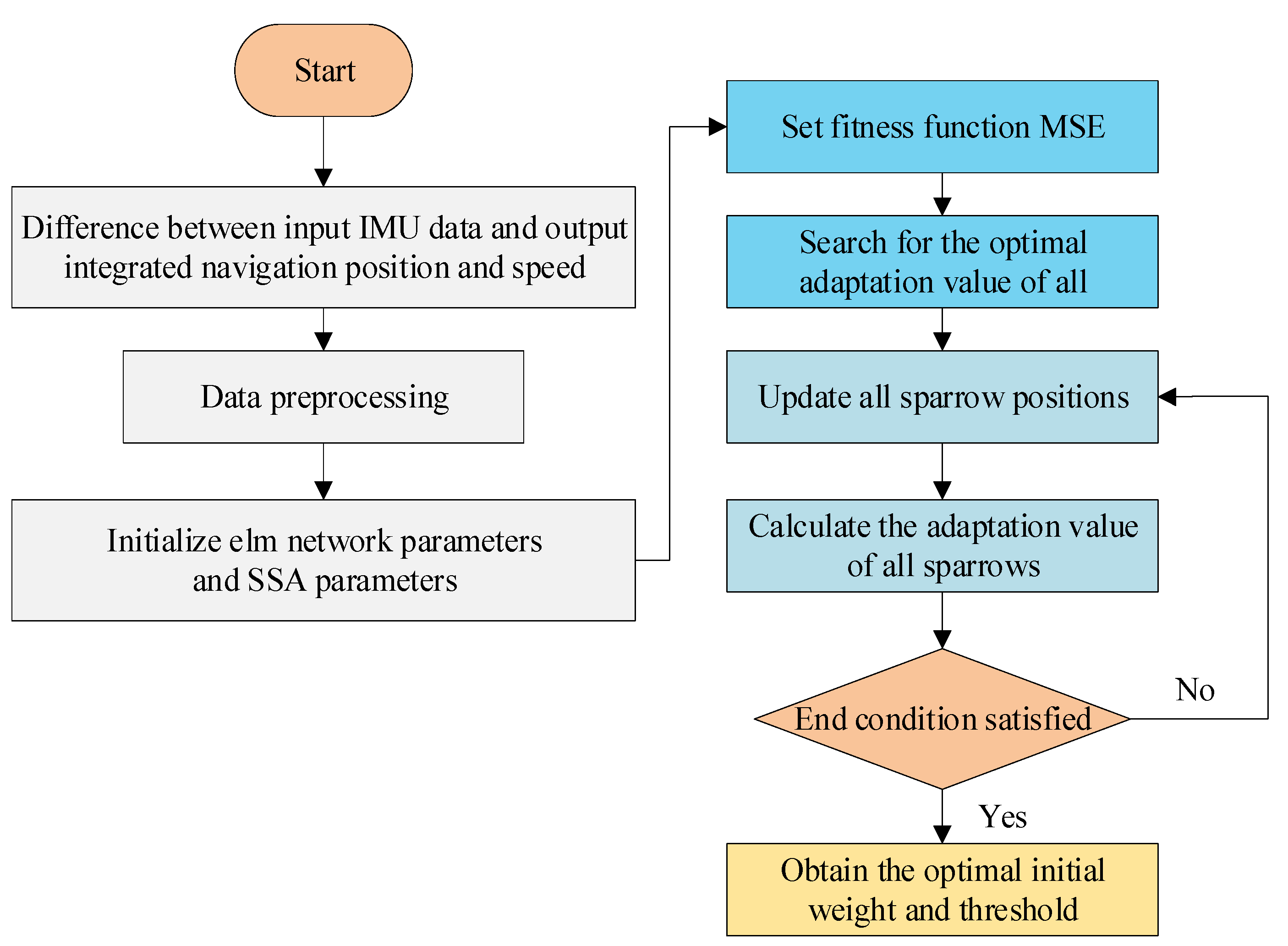
The flow chart of the SSA-ELM algorithm is shown in Figure 6. The INS/GPS integrated navigation data is first preprocessed, and the optimal weight and threshold for ELM are found using the SSA-ELM model. We use the neural network for training. Since the initial weight and threshold of the ELM neural network are randomly generated, the selection of the initial weight and threshold is vital for the learning ability of ELM. Furthermore, SSA has the advantages of strong optimization capacity and fast convergence speed. Thus, in this paper, a learning algorithm based on an SSA is proposed to optimize the ELM, and the initial weight and threshold of the ELM algorithm are optimized by SSA algorithm. The steps of the SSA-ELM model are as follows:
1.
The three-axis acceleration and angular velocity are obtained after noise removal and confirmed as input after data processing. Subsequently, they are output as the INS position and velocity errors.
2.
The SSA and ELM parameters, sample weights, and output weights are initialized. The MSE of ELM is obtained through calculation, the fitness function is selected, and the fitness value is calculated, as shown in (28). The MSE after ELM training is taken as the SSA fitness value.
3.
The fitness value corresponding to each sparrow and the sparrow position corresponding to the best fitness are calculated using the SSA (see (17–21)), and iteration is done to update the best fitness value and position.
f i t n e s s = a r g   m i n M S E p r e d i c t
4.
We determine whether the updated optimal position and adaptation value meet the maximum number of iterations. Subsequently, the optimal initial weight and threshold of ELM are obtained, and the ELM algorithm is used for prediction.

4. Results and Discussion

4.1. Experiment

In this experiment, when GPS works normally, the SSA-ELM model is trained using GPS and INS, and when GPS is interrupted, the SSA-ELM model that has been trained is used to predict navigation error. In the experiment, the sensor parameters are presented in Table 2. The interruption scheme is divided into four steps: low-speed straight-line navigation, high-speed steering, low-speed steering, high-speed straight-line navigation. As shown in Figure 7, these schemes are denoted by yellow, purple, blue and red lines, respectively. The experimental time is 850 s, and GPS data are hidden to simulate GPS interruption. In the experiment, the neural network predicts the velocity and position differences of integrated navigation during GPS interruption. Moreover, it inputs the predicted velocity and position difference value and INS information into the EKF to correct the velocity and position error of the INS. The designed navigation, GPS training, and GPS interruption times are shown in Table 3. During GPS interruption, SSA-ELM corrects the INS error using a trained neural network and replaces the GPS information with the velocity and position error information provided by SSA-ELM. The neural network input includes the IMU three-axis acceleration and three-axis angular velocity, and the output is the INS velocity and position error. The input is six neurons, and the output is one neuron.
Different test times are selected to interrupt the GPS artificially, indicating that the GPS is stopped. The GPS interruption times are 30, 60, 30, and 60 s in the high-speed steering phase, the low-speed steering phase, high-speed straight-line navigation phase, and low-speed straight-line navigation phase, respectively. The neural network is trained when the GPS is normally functioning. The neural network is tested when the GPS is interrupted. The normal duration is the training set, and the interruption is the test set.
The SSA-ELM algorithm proposed in this paper is compared with pure INS, BP (back propagation) neural network, and ELM. BP is a multilayer feedforward neural network trained according to the error back propagation algorithm, and is one of the most widely used neural network models. For the above tests, RMSE and MAE are introduced to evaluate the results:
R M S E = 1 m i = 1 m ( y i y ^ i ) 2
M A E = 1 m i = 1 m ( y i y ^ i )
In the above formulae, y ^ i is the predicted value estimated by the neural network, y i is the true value, y ¯ i is the average value of the true value, and m is the number of predicted result data.

4.2. EEMD Denoising

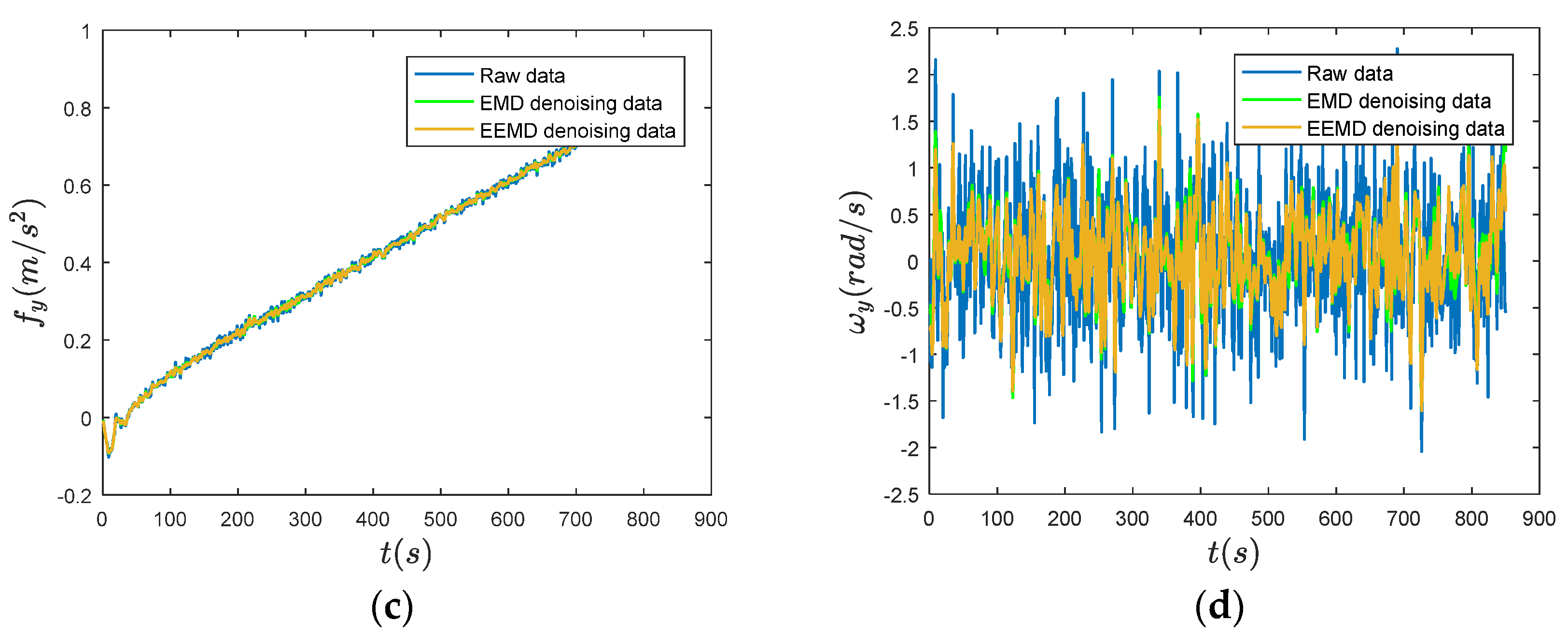
To suppress the influence of the IMU noise on the inertial navigation, a denoising method based on EEMD is adopted to denoise the three-axis angular velocity and acceleration of IMU and compare the de-noising results with the EMD de-noising results. The results demonstrate that EEMD can effectively suppress the modal aliasing of EMD. The standard deviation of adding Gaussian white noise to EEMD is set to 0.2, and the number of white noises is set to 100. Figure 8 reveals the denoising results of EMD and EEMD on three axes x , y for specific force and angular velocity, respectively. The original data are represented by a blue line, the EMD-denoised data are represented by a green line, and the EEMD-denoised data are represented by a red line. The denoising effects of EMD and EEMD evaluated by RMSE and PSNR are shown in Table 4 and Table 5. The tables show that EEMD has a better denoising effect on the IMU than EMD. The signal-to-noise ratio of the original signal can be improved through EEMD and input the IMU measurement value after noise removal into INS to obtain an accurate navigation solution. Additionally, EEMD provides accurate measurement information for integrated navigation and improves the prediction ability of the neural network during GPS interruption, ultimately improving the accuracy of integrated navigation.

4.3. SSA-ELM

In the SSA-ELM model, the input layer is a six-dimensional vector, the output layer is a one-dimensional vector, the activation function of the hidden layer is a ReLU function, the sparrow population size is 20, the number of iterations is 100, the proportion of discoverers in the population is 20%, the proportion of vigilantes in the population is 10%, and the safety threshold ST is 0.8.
The first 600 s of the IMU and GPS output are used in the training phase. The GPS interruption times in the high- and low-speed steering phases and the high- and low-speed straight-line navigation phases are 30 s, 60 s, 30 s, and 60 s, respectively. When GPS is interrupted and measurement information cannot be provided, the SSA-ELM model is used to train the measurement information with the GPS signal, predict the current measurement information, and integrate INS and GPS as the inputs of EKF. Furthermore, the prediction model of SSA-ELM is verified, and the error is analyzed.
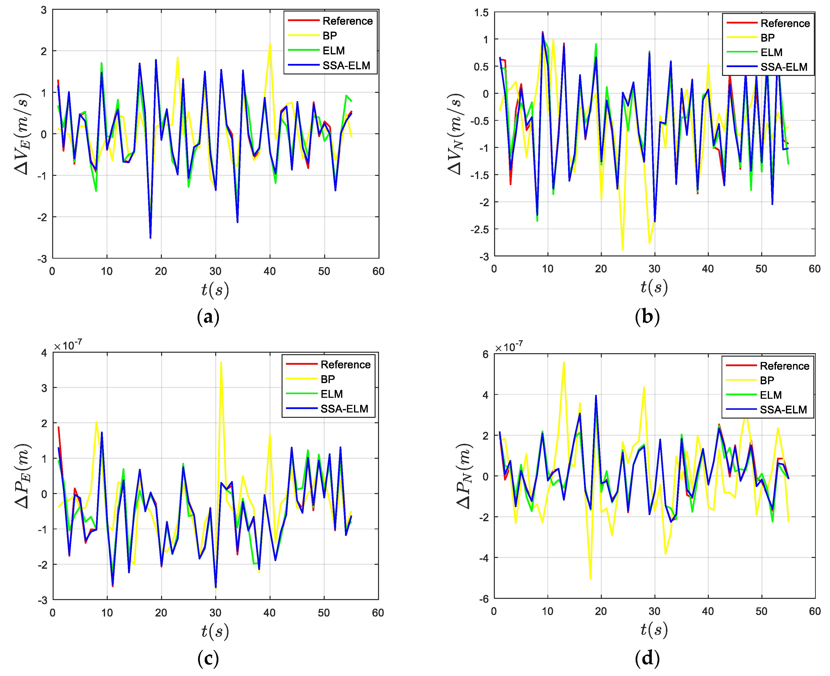
In the high-speed steering phase, the network is trained using the IMU output and GPS information, and the difference between east and north velocity and position are predicted through the trained network in 30 s during the first interruption. Figure 9 shows the east and north velocity and position differences during the first interruption. Table 6 lists the RMSE and MAE of the velocity and position differences in the east and north directions between the SSA-ELM model and the BP and ELM models. The results show that the SSA-ELM model effectively predicts the INS/GPS velocity and position differences. In RMSE, compared with the BP model, the prediction accuracy of the east velocity difference and the north velocity difference improved by 79.9% and 83.2%, respectively, and improved by 45.4% and 51%, respectively, compared with ELM. Meanwhile, compared with the BP model, the east and north position differences increased by 85.7% and 86.4%, respectively, and by 37% and 67.3%, respectively, compared with ELM. In MAE, compared with the BP model, the prediction accuracy of the east and north velocity difference improved by 84.2% and 82.6%, respectively, and by 58.8% and 55.2%, respectively, compared with ELM. In addition, the east and north position differences increased by 89.3% and 86.5%, respectively, compared with the BP model and by 54.6% and 69.4%, respectively, compared with ELM.
In the low-speed steering phase, the network is trained using the IMU output and GPS information. and the difference between east and north velocity and position are predicted through the trained network in 60 s during the second interruption. Figure 10 shows the east–north velocity and position differences during the second interruption. Table 7 shows the RMSE and MAE of the velocity and position differences in the east and north directions between the SSA-ELM model and the BP and ELM models. The results show that the SSA-ELM model effectively predicts the INS/GPS velocity and position differences. In RMSE, compared with the BP model, the prediction accuracy of the east and north velocity difference is improved by 91.5% and 84.9%, respectively, and by 73% and 31.4%, respectively, compared with ELM. Meanwhile, compared with the BP model, the east and north position differences increased by 89.3% and 93.1%, respectively, and by 69.4% and 71.6%, respectively, compared with ELM. In MAE, compared with the BP model, the prediction accuracy of the east degree difference and the north velocity difference improved by 91.8% and 86.7%, respectively, and by 76.5% and 48.7%, respectively, compared with ELM. In addition, the east and north position differences increased by 91% and 93.6%, respectively, compared with the BP model, and by 73.3% and 71.8%, respectively, compared with ELM.
In the high-speed straight-line navigation phase, the network is trained using the IMU output and GPS information. and the difference between east and north velocity and position are predicted through the trained network in 30 s during the third interruption. Figure 11 shows the east and north velocity and position differences during the third interruption. Table 8 shows the RMSE and MAE of the velocity and position differences in the east and north directions between the SSA-ELM model and the BP and ELM models. The results show that the SSA-ELM model effectively predicts INS/GPS velocity and position differences. In RMSE, compared with the BP model, the prediction accuracy of the east and north velocity difference improved by 89.8% and 96.3%, respectively, and by 68.7% and 79.6%, respectively, compared with ELM. Simultaneously, compared with the BP model, the east and north position differences increased by 99.2% and 93.5%, respectively, and by 76.4% and 86.1%, respectively, compared with ELM. In MAE, compared with the BP model, the prediction accuracy of the east and north velocity difference improved by 91.7% and 97.3%, respectively, and by 74.9% and 83.2%, respectively, compared with ELM. In addition, the east and north position differences increased by 91.5% and 93.9%, respectively, compared with the BP model, and by 77.2% and 88.1%, respectively, compared with ELM.
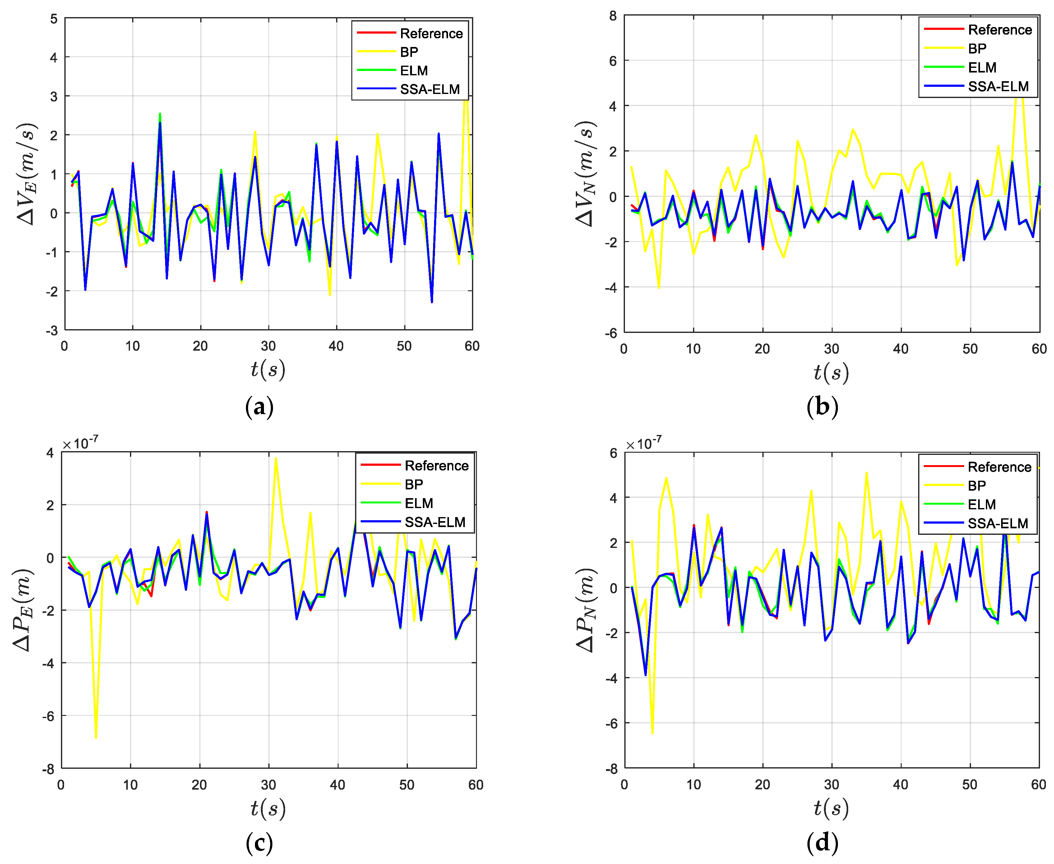
In the low-speed straight-line navigation phase, the network is trained using the IMU output and GPS information. and the difference between east and north velocity and position are predicted through the trained network in 60 s during the fourth interruption. Figure 12 shows the east and north velocity and position differences during the fourth interruption. Table 9 shows the RMSE and MAE of the velocity and position differences in the east and north directions between the SSA-ELM model and the BP and ELM models. The results show that the SSA-ELM model effectively predicts the INS/GPS velocity and position differences. In RMSE, compared with the BP model, the prediction accuracy of the east and north velocity differences improved by 96.2% and 96.2%, respectively, and improved by 88% and 60.3%, respectively, compared with ELM. Compared with the BP model, the east and north position differences increased by 93.06% and 97.7%, respectively, and by 40.9% and 77.3%, respectively, compared with ELM. In MAE, compared with the BP model, the prediction accuracy of the east and north velocity differences improved by 96.6% and 97.4%, respectively, and by 88.3% and 70.5%, respectively, compared with ELM. In addition, the east and north position differences increased by 95.3% and 98.3%, respectively, compared with the BP model, and by 65.4% and 80.3%, respectively, compared with ELM.

5. Conclusions

A neural network method based on EEMD and SSA-ELM are proposed to improve the positioning accuracy of GPS during an interruption in this study. The EEMD method can tackle IMU noise in a dynamic environment and improve the accuracy of INS equipment. The SSA-ELM model can optimize the initial weight and threshold of the ELM model and improve the prediction ability of the neural network. This provides a reliable navigation scheme for INS/GPS integrated navigation during GPS interruption. Future research may consider the addition of sensors to increase the accuracy and stability of the INS/GPS integrated navigation system. Combining the algorithm proposed in this paper with other new algorithms may be considered in order to achieve better results.

Author Contributions

Conceptualization, J.X., Y.L. and C.Z.; methodology, J.X.; validation, Z.Z. and C.Z.; writing—original draft preparation, J.X. and C.Z. All authors have read and agreed to the published version of the manuscript.

Funding

This work was supported by National Key R&D Program of China (2021YFC2800100) and Liaoning Revitalization Talents Program (XLYC2001002) and Applied Basic Research Plan of Liaoning Province in 2022 (2022JH2/101300265).

Acknowledgments

We are very grateful to the reviewers for their valuable comments that helped to improve the paper.

Conflicts of Interest

The authors declare no conflict of interest.

References

  1. Zhang, C.; Cao, C.; Guo, C.; Li, T.; Guo, M. Navigation multisensor fault diagnosis approach for an unmanned surface vessel adopted particle-filter method. IEEE Sens. J. 2021, 21, 27093–27105. [Google Scholar] [CrossRef]
  2. Noureldin, A.; Karamat, T.B.; Eberts, M.D.; EI-Shafie, A. Performance Enhancement of MEMS-Based INS/GPS Integration for Low-Cost Navigation Applications. IEEE Trans. Veh. Technol. 2009, 58, 1077–1096. [Google Scholar] [CrossRef]
  3. Bao, J.; Li, D.; Qiao, X.; Rauschenbach, T. Integrated navigation for autonomous underwater vehicles in aquaculture: A review. Inf. Process. Agric. 2020, 7, 139–151. [Google Scholar] [CrossRef]
  4. Ansari-Rad, S.; Hashemi, M.; Salarieh, H. Pseudo DVL reconstruction by an evolutionary TS-fuzzy algorithm for ocean vehicles. Measurement 2019, 147, 106831. [Google Scholar] [CrossRef]
  5. Atia, M.M.; Liu, S.; Nematallah, H.; Karamat, T.B.; Noureldin, A. Integrated indoor navigation system for ground vehicles with automatic 3-D alignment and position initialization. IEEE Trans. Veh. Technol. 2015, 64, 1279–1292. [Google Scholar] [CrossRef]
  6. Mu, X.; He, B.; Wu, S.; Zhang, X.; Song, Y.; Yan, T. A practical INS/GPS/DVL/PS integrated navigation algorithm and its application on Autonomous Underwater Vehicle. Appl. Ocean Res. 2020, 106, 102441. [Google Scholar] [CrossRef]
  7. Xu, Q.; Li, X.; Chan, C.Y. Enhancing localization accuracy of MEMS-INS/GPS/in-vehicle sensors integration during GPS outages. IEEE Trans. Instrum. Meas. 2018, 67, 1966–1978. [Google Scholar] [CrossRef]
  8. Liu, Y.; Fan, X.; Lv, C.; Wu, J.; Li, L.; Ding, D. An innovative information fusion method with adaptive Kalman filter for integrated INS/GPS navigation of autonomous vehicles. Mech. Syst. Signal Process. 2018, 100, 605–616. [Google Scholar] [CrossRef] [Green Version]
  9. Wang, Q.; Liu, S.; Zhang, B.; Zhang, C. FBLS-Based Fusion Method for Unmanned Surface Vessel Positioning Considering Denoising Algorithm. J. Mar. Sci. Eng. 2022, 10, 905. [Google Scholar] [CrossRef]
  10. Silson, P.M.G. Coarse Alignment of a Ship’s Strapdown Inertial Attitude Reference System Using Velocity Loci. IEEE Trans. Instrum. Meas. 2011, 60, 1930–1941. [Google Scholar] [CrossRef]
  11. Li, J.; Song, N.; Yang, G.; Li, M.; Cai, Q. Improving positioning accuracy of vehicular navigation system during GPS outages utilizing ensemble learning algorithm. Inf. Fus. 2017, 35, 1–10. [Google Scholar] [CrossRef]
  12. Godha, S.; Cannon, M.E. GPS/MEMS INS integrated system for navigation in urban areas. GPS Solut. 2007, 11, 193–203. [Google Scholar] [CrossRef]
  13. Tang, J.; Fu, Z.; Deng, Z. Identification method for RLG random errors based on Allan variance and equivalent theorem. Chin. J. Aeronaut. 2009, 22, 273–278. [Google Scholar] [CrossRef] [Green Version]
  14. Song, J.; Shi, Z.; Du, B.; Han, L.; Wang, H.; Wang, Z. MEMS gyroscope wavelet de-noising method based on redundancy and sparse representation. Microelectron. Eng. 2019, 217, 111112. [Google Scholar] [CrossRef]
  15. Eftekhari, H.R.; Ghatee, M. Hybrid of discrete wavelet transform and adaptive neuro fuzzy inference system for overall driving behavior recognition. Transport. Res.–Traf. Psychol. Behav. 2018, 58, 1369–8478. [Google Scholar] [CrossRef]
  16. Yang, X.H.; Ren, J.X.; Zhao, X.M.; Chen, R. MEMS gyro signal de-noising based on adaptive stationary wavelet threshold. Adv. Mater. Res. 2012, 466, 986–990. [Google Scholar] [CrossRef]
  17. Sheng, G.; Gao, G.; Zhang, B. Application of improved wavelet thresholding method and an RBF network in the error compensating of an MEMS gyroscope. Micromachines 2019, 10, 608. [Google Scholar] [CrossRef] [Green Version]
  18. Abdolkarimi, E.S.; Mosavi, M.R. A low-cost integrated MEMS-based INS/GPS vehicle navigation system with challenging conditions based on an optimized IT2FNN in occluded environments. GPS Solut. 2020, 24, 108. [Google Scholar] [CrossRef]
  19. Liu, H.; Jia, J.; Lin, Z.; Wang, Z.; Gong, H. Relationship between net primary production and climate change in different vegetation zones based on EEMD detrending—A case study of Northwest China. Ecol. Indic. 2021, 122, 107276–107287. [Google Scholar] [CrossRef]
  20. Wu, Z.; Wang, W. INS/magnetometer integrated positioning based on neural network for bridging long-time GPS outages. GPS Solut. 2019, 23, 88. [Google Scholar] [CrossRef]
  21. Chen, X.; Shen, C.; Zhang, W.; Tomizuka, M.; Xu, Y.; Chiu, K. Novel hybrid of strong tracking Kalman filter and wavelet neural network for GPS/INS during GPS outages. Measurement 2013, 46, 3847–3854. [Google Scholar] [CrossRef]
  22. Liu, F.; Sun, X.; Xiong, Y.; Huang, H.; Guo, X.; Zhang, Y.; Shen, C. Combination of iterated cubature Kalman filter and neural networks for GPS/INS during GPS outages. Rev. Sci. Instrum. 2019, 90, 125005–1250015. [Google Scholar] [CrossRef]
  23. Chen, L.; Fang, J. A hybrid prediction method for bridging GPS outages in high-precision POS application. IEEE Trans. Instrum. Meas. 2014, 63, 1656–1665. [Google Scholar] [CrossRef]
  24. Shen, C.; Zhang, Y.; Tang, J.; Cao, H.; Liu, J. Dual-optimization for a MEMS-INS/GPS system during GPS outages based on the cubature Kalman filter and neural networks. Mech. Syst. Signal. Process. 2019, 133, 106222–106235. [Google Scholar] [CrossRef]
  25. Belhajem, I.; Maissa, Y.B.; Tamtaoui, A. Improving vehicle localization in a smart city with low cost sensor networks and support vector machines. Mob. Netw. Appl. 2018, 23, 854–863. [Google Scholar] [CrossRef]
  26. Zhi, Z.A.; Liu, D.; Liu, L. A performance compensation method for GPS/INS integrated navigation system based on CNN–LSTM during GPS outages. Measurement 2022, 188, 110516–110530. [Google Scholar] [CrossRef]
  27. Fu, Q.; Jing, B.; He, P.; Si, S.; Wang, Y. Fault Feature Selection and Diagnosis of Rolling Bearings Based on EEMD and Optimized. IEEE Sens. J. 2018, 18, 5024–5034. [Google Scholar] [CrossRef]
  28. Li, S.; Qin, N.; Huang, D.; Huang, D.; Ke, L. Damage Localization of Stacker’s Track Based on EEMD-EMD and DBSCAN Cluster Algorithms. IEEE Trans. Instrum. Meas. 2019, 69, 1981–1992. [Google Scholar] [CrossRef]
  29. Wu, Z.; Huang, N.E. A study of the characteristics of white noise using the empirical mode decomposition method. Proc. Roy. Soc. London A. 2003, 460, 1597–1611. [Google Scholar] [CrossRef]
  30. Liu, Z.; Cui, Y.; Li, W. A Classification Method for Complex Power Quality Disturbances Using EEMD and Rank Wavelet SVM. IEEE Trans. Smart. Grid. 2015, 6, 1678–1685. [Google Scholar] [CrossRef]
  31. Xue, J.; Shen, B. A novel swarm intelligence optimization approach: Sparrow search algorithm. Syst. Sci. Control Eng. 2020, 8, 22–34. [Google Scholar] [CrossRef]
  32. Huang, G.B.; Wang, D.H.; Lan, Y. Extreme learning machines: A survey. Int. J. Mach. Learn. Cyb. 2011, 2, 107–122. [Google Scholar] [CrossRef]
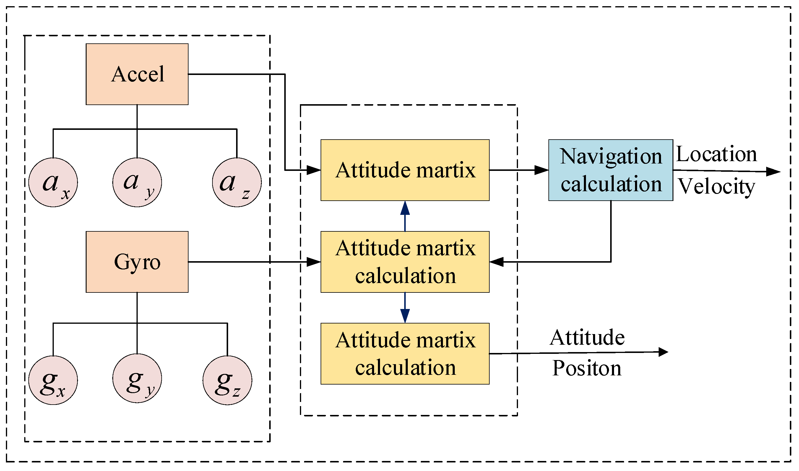
Figure 1. Inertial navigation system (INS) solution diagram.
Jmse 10 01733 g001
Figure 2. Training mode.
Jmse 10 01733 g002
Figure 3. Prediction mode.
Jmse 10 01733 g003
Figure 4. Ensemble empirical mode decomposition (EEMD) process.
Jmse 10 01733 g004
Figure 5. Extreme learning machine (ELM) model.
Jmse 10 01733 g005
Figure 6. Sparrow search algorithm (SSA)-ELM algorithm flow chart.
Jmse 10 01733 g006
Figure 7. Ship track chart.
Jmse 10 01733 g007
Figure 8. Comparison of specific force and angular velocity denoising effects: (a) specific force denoising effect in x−axis; (b) angular velocity denoising effect in x−axis; (c) specific force denoising effect in y−axis; (d) angular velocity denoising effect in y−axis.
Jmse 10 01733 g008aJmse 10 01733 g008b
Figure 9. Prediction of the velocity and position differences of different methods during the first interruption: (a) east velocity difference prediction; (b) north velocity difference prediction; (c) east position difference prediction; (d) north position difference prediction.
Jmse 10 01733 g009
Figure 10. Velocity and position difference prediction of different methods during the second interruption: (a) east velocity difference prediction; (b) north velocity difference prediction; (c) east position difference prediction; (d) north position difference prediction.
Jmse 10 01733 g010
Figure 11. Prediction of the velocity and position differences of different methods during the third interruption: (a) east velocity difference prediction; (b) north velocity difference prediction; (c) east position difference prediction; (d) north position difference prediction.
Jmse 10 01733 g011
Figure 12. Prediction of the velocity and position differences of different methods during the fourth interruption: (a) east velocity difference prediction, (b) north velocity difference prediction, (c) east position difference prediction, and (d) north position difference prediction.
Jmse 10 01733 g012
Table 1. Criteria for judging the degree of relevance.
Related CoefficientDegree of Correlation
0 < r < 0.3 no linear relationship
0.3 r < 0.5 low-degree linear relationship
0.5 r 0.8 significant linear relationship
r > 0.8 highly linear relationship
Table 2. Parameters of sensors.
Experimental EquipmentMain ParameterValue
 
Accelerometer
 
 
Gyroscope
 
Resolving power
Zero bias
Roman walk
resolving power
Zero bias
Roman walk
0.3 mg
0.2 mg
0.2 m/s h
0.07°/s
0.07°/s
1.9 s/ h
 
GPS
 
GPS update rate
Velocity error
Position error
1 Hz
0.1 m/s
2 m
Table 3. Setting of GPS interruption during prediction.
SchemeSailing Time
(s)
GPS Training Time
(s)
GPS Interruption Time
(s)
high-speed steering phase0–8500–85030
low-speed steering phase0–8500–85060
high-speed straight-line navigation phase0–8500–85030
low-speed straight-line navigation phase0–8500–85060
Table 4. RMSE effect evaluation.
ω x ω y f x f y
EMD denoising0.59040.56520.02970.0069
EEMD denoising0.58470.55340.02960.0063
Table 5. PSNR effect evaluation.
ω x ω y f x f y
EMD denoising4.57784.955730.537043.2673
EEMD denoising4.66095.139830.546344.0195
Table 6. RMSE and MAE of the velocity and position differences of different methods during the first interruption.
Error IndicatorBPELMSSA-ELM
Δ V E /m/sRMSE
MAE
1.0878
0.7920
0.4006
0.3036
0.2186
0.1252
Δ V N /m/sRMSE
MAE
1.2776
0.8443
0.4392
0.3271
0.2151
0.1467
Δ P E / m RMSE
MAE
1.7131 × 10⁻⁶
1.2222 × 10⁻⁷
3.8987 × 10⁻⁸
2.8924 × 10⁻⁸
2.4579 × 10⁻⁸
1.3118 × 10⁻⁸
Δ P N / m RMSE
MAE
1.4452 × 10⁻⁷
9.7608 × 10⁻⁸
5.9862 × 10⁻⁸
4.3075 × 10⁻⁸
1.9601 × 10⁻⁸
1.3199 × 10⁻⁸
Table 7. RMSE and MAE of the velocity and position differences of different methods during the second interruption.
Error IndicatorBPELMSSA-ELM
Δ V E /m/sRMSE
MAE
0.8561
0.5968
0.2713
0.2097
0.0732
0.0492
Δ V N /m/sRMSE
MAE
0.9955
0.6615
0.2188
0.1713
0.1502
0.0879
Δ P E / m RMSE
MAE
1.0118 × 10⁻⁷
6.9115 × 10⁻⁸
3.5438 × 10⁻⁸
2.3357 × 10⁻⁸
1.0840 × 10⁻⁸
6.2258 × 10⁻⁹
Δ P N / m RMSE
MAE
1.9017 × 10⁻⁷
1.4695 × 10⁻⁷
4.6257 × 10⁻⁸
3.3467 × 10⁻⁸
1.3135 × 10⁻⁸
9.4451 × 10⁻⁹
Table 8. RMSE and MAE of the velocity and position differences of different methods during the third interruption.
Error IndicatorBPELMSSA-ELM
Δ V E /m/sRMSE
MAE
0.9642
0.6691
0.3144
0.2209
0.0983
0.0555
Δ V N /m/sRMSE
MAE
1.3712
1.1762
0.2460
0.1886
0.0503
0.0316
Δ P E / m RMSE
MAE
8.2396 × 10⁻⁷
5.5197 × 10⁻⁸
2.9593 × 10⁻⁸
2.0574 × 10⁻⁸
6.9779 × 10⁻⁹
4.6938 × 10⁻⁹
Δ P N / m RMSE
MAE
1.0313 × 10⁻⁷
7.4401 × 10⁻⁸
4.7877 × 10⁻⁸
3.8411 × 10⁻⁸
6.6536 × 10⁻⁹
4.5647 × 10⁻⁹
Table 9. RMSE and MAE of the velocity and position differences of different methods during the fourth interruption.
Error IndicatorBPELMSSA-ELM
Δ V E /m/sRMSE
MAE
0.8471
0.5344
0.2698
0.1554
0.0323
0.0182
Δ V N /m/sRMSE
MAE
2.1322
1.6591
0.2016
0.1446
0.0801
0.0426
Δ P E / m RMSE
MAE
1.4343 × 10⁻⁷
8.2507 × 10⁻⁸
1.6845 × 10⁻⁸
1.1292 × 10⁻⁸
9.9519 × 10⁻⁹
3.9092 × 10⁻⁹
Δ P N / m RMSE
MAE
2.6129 × 10⁻⁷
2.0455 × 10⁻⁷
2.7082 × 10⁻⁸
1.7762 × 10⁻⁸
6.1381 × 10⁻⁹
3.4930 × 10⁻⁹
Publisher’s Note: MDPI stays neutral with regard to jurisdictional claims in published maps and institutional affiliations.