Application of Singularity Theory to the Distribution of Heavy Metals in Surface Sediments of the Zhongsha Islands

Abstract

This research aimed to use nonlinear theory and technology to describe the spatial distribution of heavy metals in the surface sediments of the Zhongsha Islands Sea region. The goal of this study is to explore the spatial distribution characteristics of heavy metals in the surface sediments of the Zhongsha Islands. The singularity theory and method were used to delineate heavy metal geochemical anomalies and the generalized self-similarity analysis method was used to decompose heavy metal geochemical anomalies and background concentrations. The results showed that there were abnormally high concentrations of heavy metals in the deep-sea plain area and in the western central sand trough area. The results of this study can inform priority areas for environmental monitoring. The element anomalies extracted by the singularity analysis method in this paper can be a guide to the next step in the investigation and provide the basis for the regional environmental assessment.

1. Introduction

In order to study the spatial distribution characteristics of heavy metal content in surface sediments of the Zhongsha Islands, the singularity analysis method was used in this paper. The Zhongsha Islands in the center of the South China Sea serve as the research study area. Previous studies on the sea area of the Zhongsha Islands mostly focused on the characteristics of trough sedimentation [1,2], structural systems [3], marine geology and geophysics [4], surface sediment analysis [5,6,7], and seawater geochemical analysis [8]. However, there has been relatively little focus on marine sediment pollution in the Zhongsha Islands, particularly on the analysis of heavy metal anomalies. The sediment heavy metal contents reflect spatiotemporal changes in pollutants [9,10,11]. Therefore, sedimentary heavy metal concentrations may be used as a proxy for the total amount of metals in a given body of water [10,12]. The contamination of an environment by heavy metals beyond a certain threshold will be more difficult to remediate [13,14]. Under these conditions, secondary pollution can occur if the hydrodynamic conditions change or heavy metals are released from the sediments and biological activities transport metals to the ecological environment [15,16]. Therefore, it is crucial to spatially examine heavy metal concentrations in marine sediments.

Dispersed elements are usually characterized by a normal or lognormal distribution [17,18,19]; the thresholds of anomalies are determined using percentages, means, and standard deviations. However, these widely applied statistical methods do not consider variability in the spatial distribution of geochemical data, particularly when there is little difference between anomalies and backgrounds. Therefore, these methods cannot effectively identify anomalies in areas with high background concentrations in heavy metals and ignore weak anomalies. Statistical techniques for analyzing spatial variability, such as geostatistics and fractal methods, may be more appropriate [20,21,22]. Many sub-disciplines within geoscience have applied fractal theory. A study by Cheng et al., 1994, on the geochemical elements concluded that they have fractal characteristics. A study by [23] Xie and Bao (2004) using the de Wijs model concluded that the geochemical domain has multifractal characteristics. Agterberg concluded that small concentrations of heavy metals represent the mixing of different groups [24] (Agterberg, 2007), whereas higher concentrations satisfy the Pareto distribution, but with a wider tail than the lognormal distribution. Cheng introduced the principle of multifractal singularity into geochemical data analysis and showed that the fractal method is more effective than traditional statistical geochemical data analysis methods for identifying heavy metal anomalies [25] (Cheng et al., 1994).

Most heavy metals are harmful to organisms. For example, heavy metals discharged with wastewater can accumulate in algae and sediment; even if the concentration is small, it can be adsorbed by fish and shellfish, resulting in food chain concentration, thus causing public hazards. In this study, if we can know which parts have high heavy metal content, it will help us to take next steps to guide environmental assessment. The present study applied the singularity theory to the observed data for the Zhongsha area collected during the Zhongsha voyage. The current study′s findings are expected to enable future research on the regional distributions of heavy metals and guide environmental management in this region. The increasing prominence of Chinese shipping has emphasized the need for coastal conservation measures in the South China Sea, such as marine environmental protection, marine fishery resources development, and maritime shipping management.

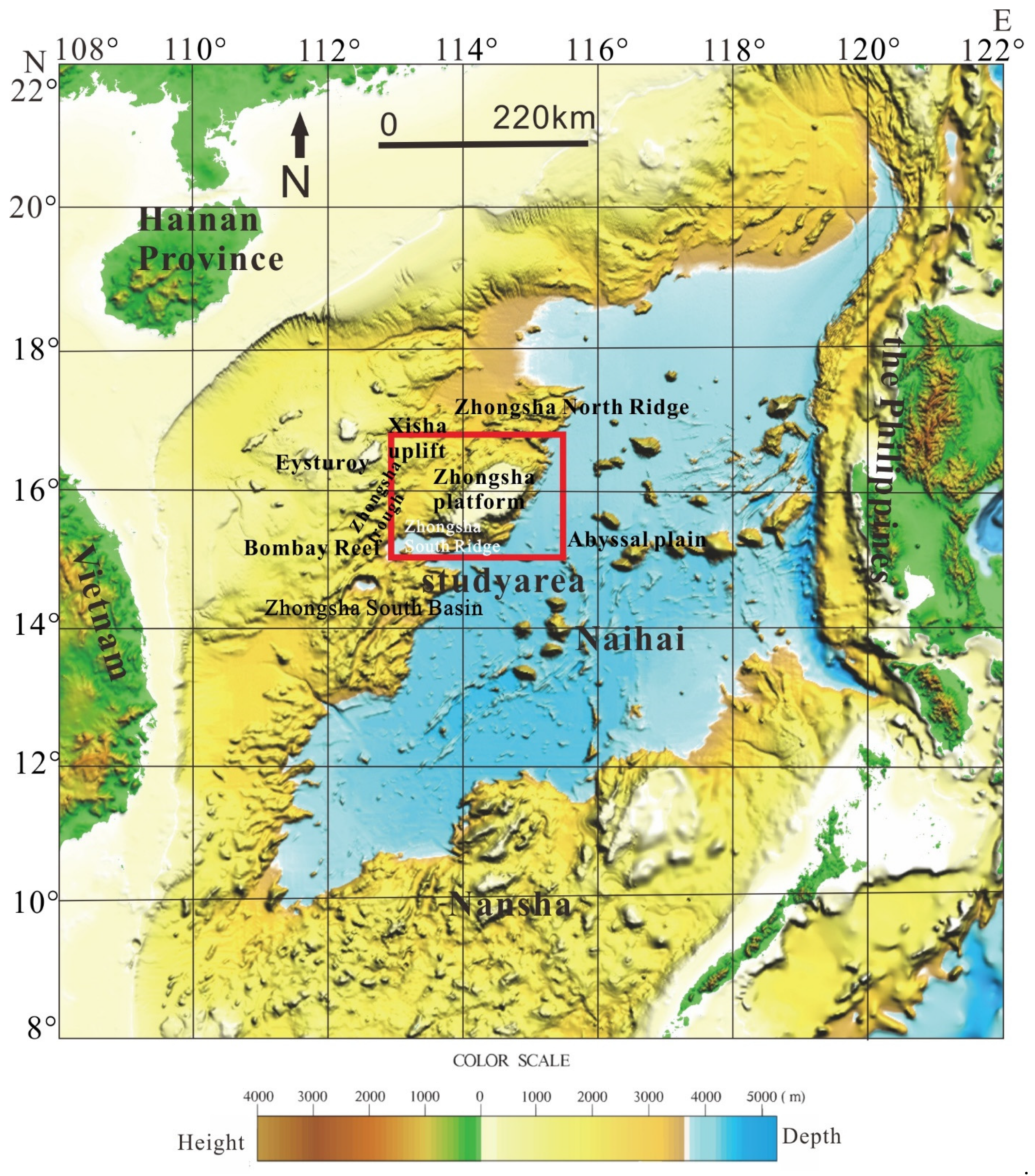
2. Study Area

The Zhongsha Islands marine region is bordered by the northwest, the eastern, and the southwestern sub basin, respectively. It is located in the South China Sea′s transition zone between the northern continental slope and the oceanic crust basin [3]. Large geomorphic units, such as the Zhongsha Platform, Xisha Uplift, Zhongsha Trough, South Zhongsha Basin, deep sea plain, North Zhongsha Ridge, and South Zhongsha Ridge, are enveloped in the study area (Figure 1). The Zhongsha Atoll [26] is in the northwest edge of the central basin. This atoll is the largest atoll in the South China Sea and has a strike direction of NE–SW and water depth of 15–600 m. The atoll has a series of dark sands and reefs and many submarine canyons. The northern part of the study area is surrounded by terraces leading to the sea slope. The Xisha Uplift is in the northwest part of the study area with a water depth of 500–2500 m. The Zhongsha Trough is at the junction of the Zhongsha Platform and Xisha Uplift, has a water depth of 2600–3200 m, is distributed in the NE–SW direction, and has a relatively flat terrain. The South Zhongsha Basin is in the southwest part of the study area, is surrounded by high terrain, and has a water depth of 3380–3840 m. The terrain inside the basin is flat.

3. Methods

3.1. Analysis of Local Singularities

The spatial distribution of geochemical anomalies comprehensively reflects the characteristics of anomalies. The analysis of geochemical anomalies can provide a much more accurate reflection of concentrations of geochemical elements and can continuously reflect multi-scale spatial changes in anomalies compared with other types of anomalies, such as geophysical anomalies. Therefore, the quantitative analysis of local structural patterns in heavy metal anomalies conducted in the present study can increase understanding of anomalies and how to identify them. The singularity index defined by multifractal theory Δα [27] can be used to measure the local scaling and singularity of anomalies. The local singularity method developed based on the singularity index can be used to delineate various types of local anomalies on multiple scales and to measure the degree of singularity.

The principle of the local singularity method is to define the field value (usually the field density) over a small range according to the scale of the field <ρ(ε)>. The field value is then split into two components:

<ρ(ε)> = cε^α−2 = cε^−Δα

(1)

In Equation (1), c is the density component related to the measurement scale unit, and has a density property that can be referred to as “fractal density” (unit g/m^α, possibly g/cm^1.5); Δα is a scale component independent of the measurement scale unit; and index α is the corresponding fractal dimension. Local singularity analysis aims to identify the fractal density c and fractal dimension α and is a measurement of the intensity or density of the field in the fractal space. The difference in spatial dimension between fractal density and normal density is represented as:

Δα = 2 − α

(2)

In Equation (2), when Δα is not an integer, the density is referred to as “fractal density”; as the range of measurement is reduced, such as ε→0, the density will tend to become infinitely large or infinitely small. For example, under a fractal density and Δα = 2 − α > 0, the density will become infinite as the measurement range is reduced (ε→0), and nonlinear singularities, such as unsmooth, unstable, and non-convergent singularities, will appear at this position. Under Δα = 2 − α ≌ 0, density is independent of the size of the measurement range. In terms of the geochemical field, Δα > 0 represents the positive singular region, corresponding to the element enrichment region, Δα < 0 (the negative singular region) corresponds to the element deficiency region, and the non-singular region corresponds to the background field. The background region generally occupies most of the geochemical field [27] The singularity index shows spatial variability, referred to as “multifractal distribution”. Various geological conditions and other factors can result in enrichment of elements to produce fractal density. Most normal data (Δα ≈ 0) conform to a normal or lognormal distribution when sampling points are evenly distributed. However, a small subset of data (Δα ≠ 0) may conform to the fractal distribution [25]. The local singularity method differs from traditional statistical methods in that the information provided by the former represents the multifractal dimension and the fractal density of the field, whereas the traditional statistical methods generally measure the density of the normal area or nonsingular data. The singularity method is a novel method that describes the characteristics of the geochemical field from a new perspective.

3.2. Multifractal Filtering Technology

The fractal method decomposes, compounds, and stacks anomalies based on the generalized self-similarity principle. The aim of the fractal method is to identify anomalies in the energy spectrum space, referred to as “energy spectrum analysis” or the “S-A” method [27]. The fractal method transforms the geochemical map into a frequency domain using Fourier transform, following which a fractal filter is constructed in the frequency domain based on generalized self-similarity, and finally information is transformed back to a spatial domain through inverse Fourier transform to obtain the decomposed anomaly and background map:

A(≥S)∝S^−β

(3)

In Equation (3), S is the energy spectral density, A(≥S) is the area in space in which the energy spectral density exceeds S, and β is the exponential coefficient of the fractal model. Under A(≥S), S adheres to the exponential relationship and the logarithms of A(≥S) and S are simultaneously plotted on the double-logarithm graph. Different linear segments on the lnS − lnA(≥S) graph represent different fractal relationships, and different value intervals of s correspond to different linear relationships. The points dividing each interval can be used to determine the threshold value of the fractal filter.

The S-A method not only separates isotropic anomalies due to geological bodies with different burial depths, but also separates anisotropic anomalies resulting from more complex geological processes.

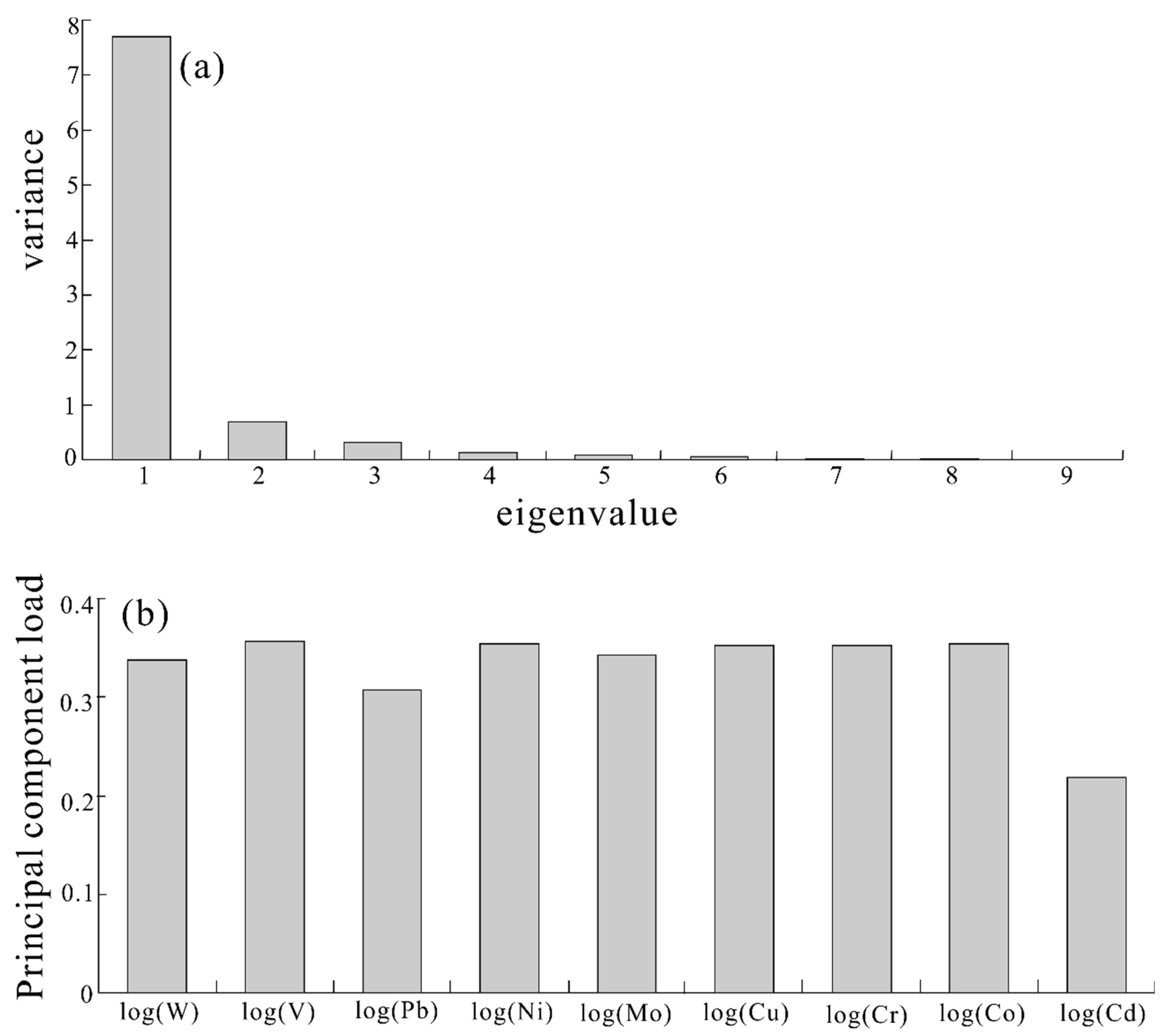
3.3. The Principal Component Analysis Method

Principal component analysis (PCA) is widely used in the analysis of geochemical anomalies for spatial delineation of geological features [28,29]. PCA is a statistical technique used to identify the geological variables that are connected and to decrease the number of variables in a dataset. The PCA algorithm is used to transform a series of interrelated geological variables into several uncorrelated geological variables through orthogonal transformation, which are referred to as principal components (PCs). Each PC is the weighted sum of all input variables. The weight of the obtained variables (the load) can be interpreted by geologists to obtain useful geological information. PCA has been a popular tool for predicting minerals in recent years [30] and environmental assessment [17,31,32,33].

4. Data Section

Data for the study area were obtained through sampling using geological equipment, mainly large-scale gravity piston, cylindrical, box, and grab samplers. The present study conducted chemical analysis and inductively coupled plasma mass spectrometry of seafloor sediments (GB/T 20260-2006). The shortest sample length of this geological sampling is 1.5 m and the longest is 5 m, both of which are surface samples. The elements were analyzed at Haikou Geological Survey Center. The elements are obtained by chemical analysis method of seabed sediment, trace and trace component analysis, and inductively coupled plasma mass spectrometry. The equipment used is an inductively coupled plasma mass spectrometer (ICAPQ).

The primary means of transport and storage for contaminants in the water are the sediments that comprise the ocean bottom. High toxicity, resistance to breakdown, and a propensity for bio-accumulation are characteristics of heavy metals. Therefore, heavy metals can have a large impact on the marine ecological environment. The present study collected 226 surface sediment samples within the boundary of the study area (see Figure 1) and the content of heavy metal elements Cu, Pb, Ni, Co, W, Mo, Cr, Cd, and V in the samples were determined.

5. Results and Discussion

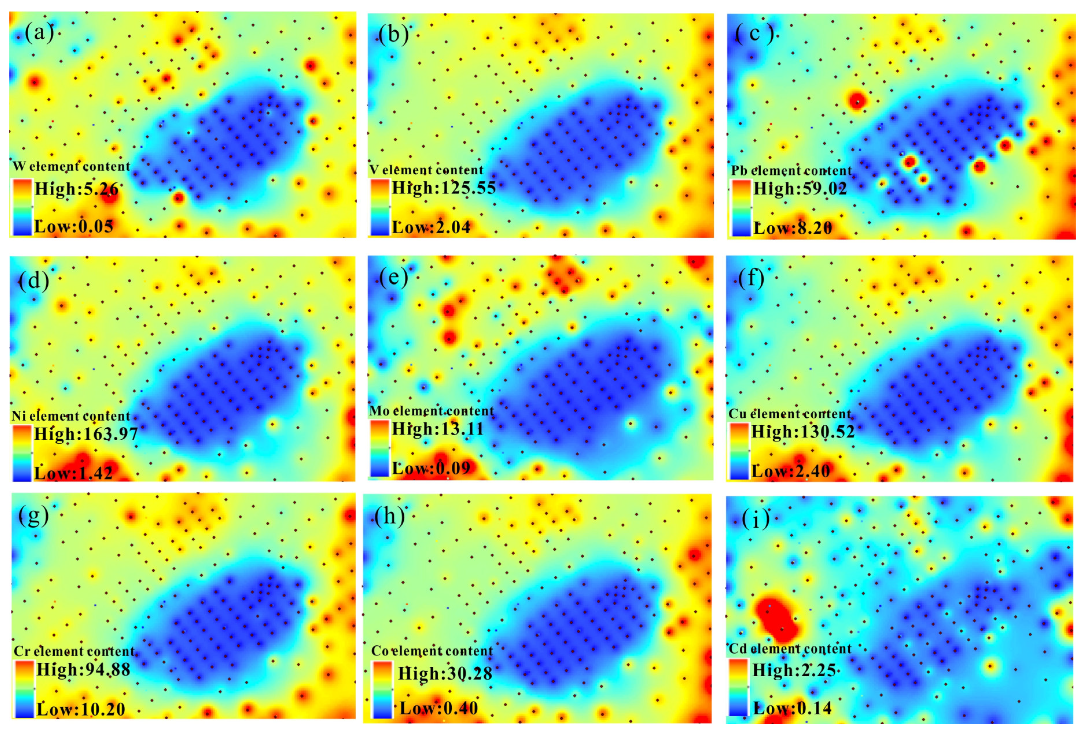
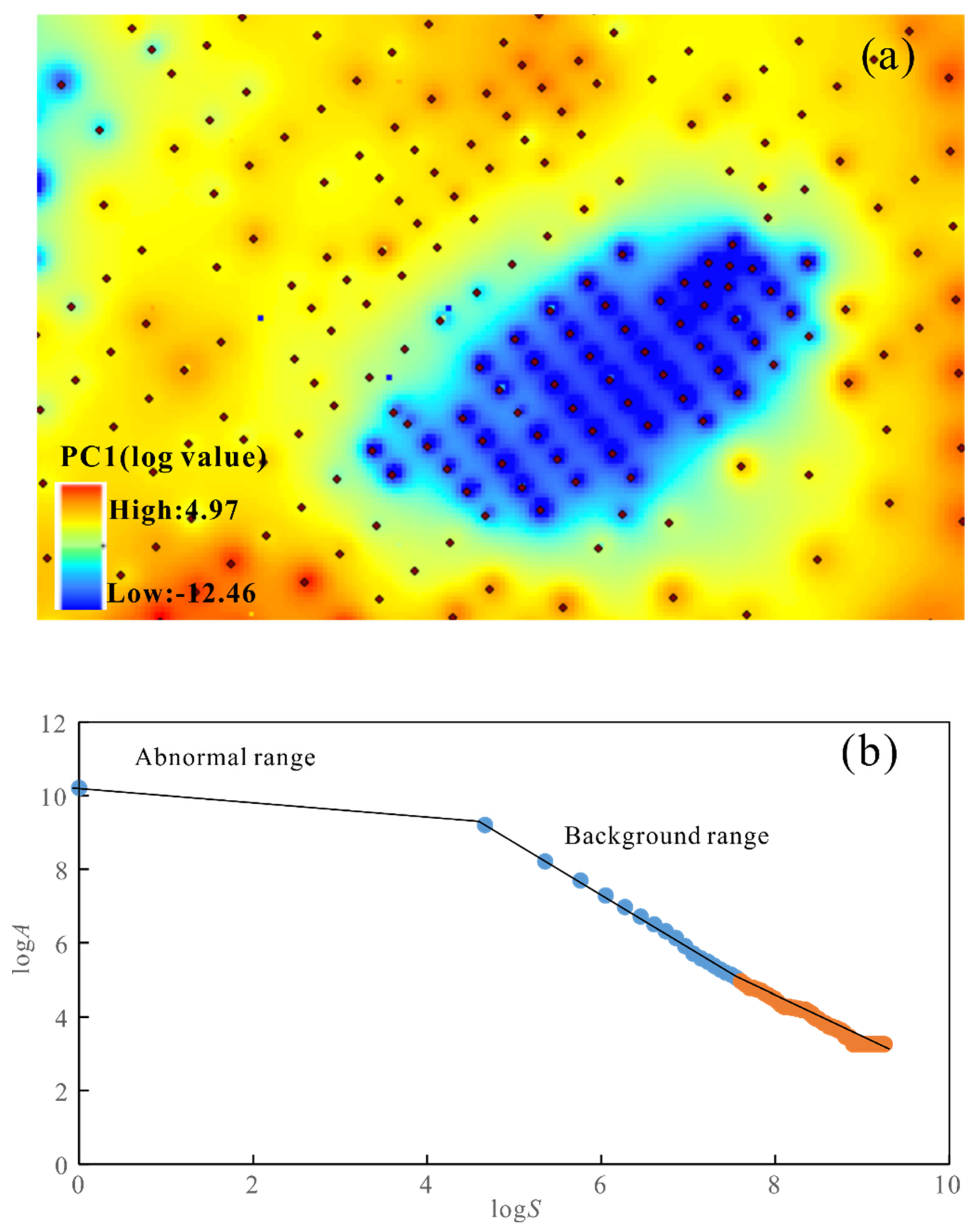
5.1. Extraction of Weak Anomalies and Delineation of Prospective Areas

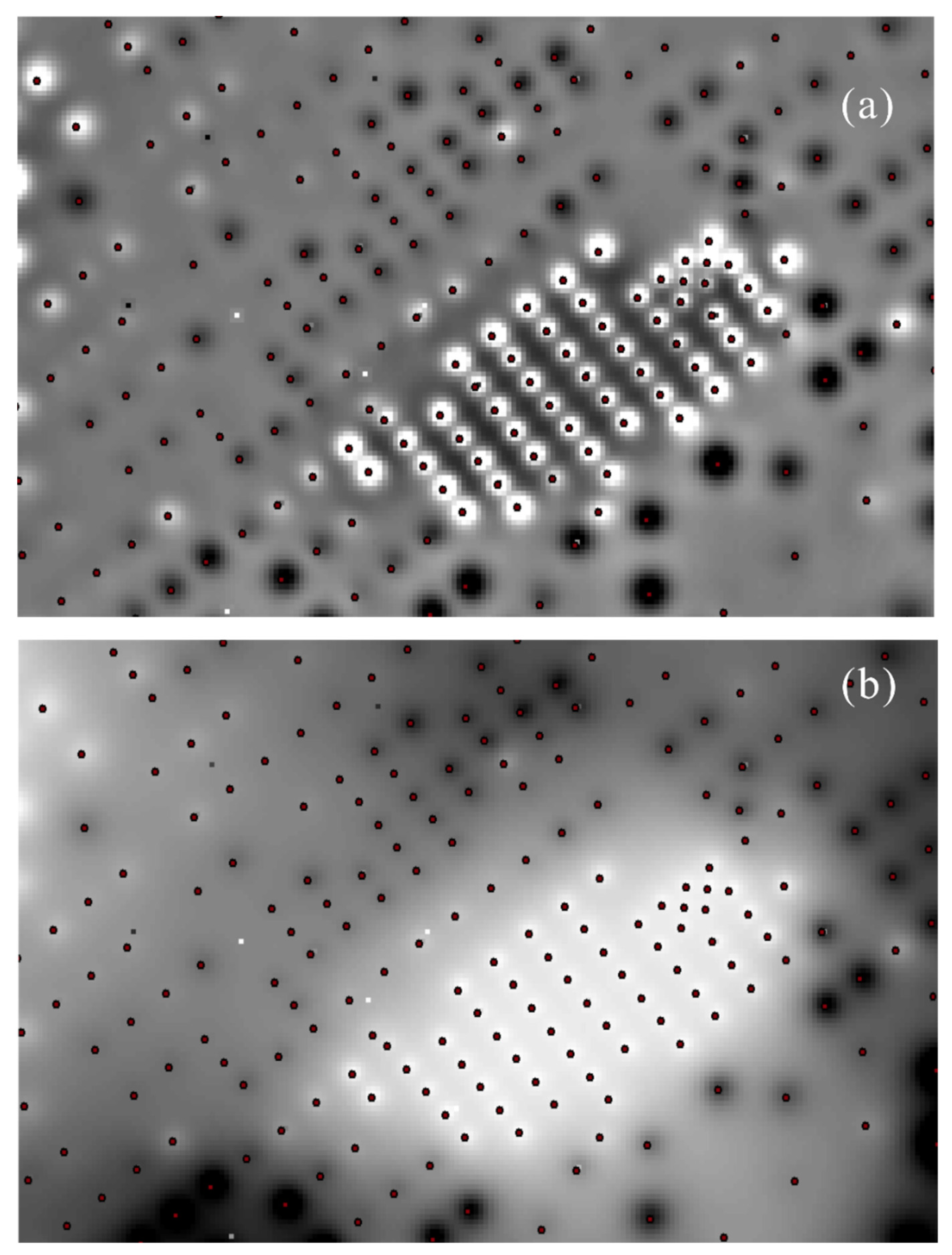
Analysis of Local Singularities and Delineation of Local Anomalies

The present study calculated the local singularity index of the spatial distributions of W, V, Pb, Ni, Mo, Cu, Cr, Co, and Cd using local singularity analysis and compiled a geochemical anomaly map to enhance and highlight local anomalies. The results showed that local singularity analysis can identify local anomalies while being relatively insensitive to the influence of background field values.

When calculating the singularity index, square windows of different sizes were formed on the geochemical map, with each point as the center, and the window sizes were (ε × ε): 2 km × 2 km, 6 km × 6 km, 10 km × 10 km, 14 km × 14 km, 26 km × 26 km. The average element density of each window was calculated, the relationship between the average density and the window size was plotted on the double logarithmic graph, and least square linear regression was applied to the data obtained from multiple windows. The slope of the regression line represented the singularity index value (Δα). The local singularity index graph was generated by mapping the local singularity index calculated at each sampling point. Figure 2 shows the distributions of W, V, Pb, Ni, Mo, Cu, Cr, Co, and Cd according to the local singularity index. As shown in Figure 3, the inverse distance ratio method with a minimum of 12 sample points and a maximum search window of 26 km × 26 km was conducted to identify the moving average of the original data for the above elements.

As shown in Figure 3, besides for the low concentrations of the nine elements W, V, Pb, Ni, Mo, Cu, Cr, Co, and Cd in the Zhongsha plateau area, higher concentrations of the elements showed scattered distributions in other parts, particularly in the deep-sea plain area in the eastern part of the study area. However, extremely high geochemical background values strongly masked possible weak and gradual anomalies around the Zhongsha Plateau, which highlights the limitations of distinguishing between the geochemical background and anomalies by concentration. As shown in Figure 2, α < 2 can clearly reflect element abnormalities, the low value region of α reflects the abnormal region of elements.

Figure 4 shows a comparison of anomalies delineated by the local singularity method and the traditional IDW method. The anomalies determined by both methods were related to the spatial distributions of known areas of high heavy metal concentrations. However, the results obtained by the singularity method also provided an improved delineation of anomalies in the uncharacterized region, indicating its greater predictive performance.

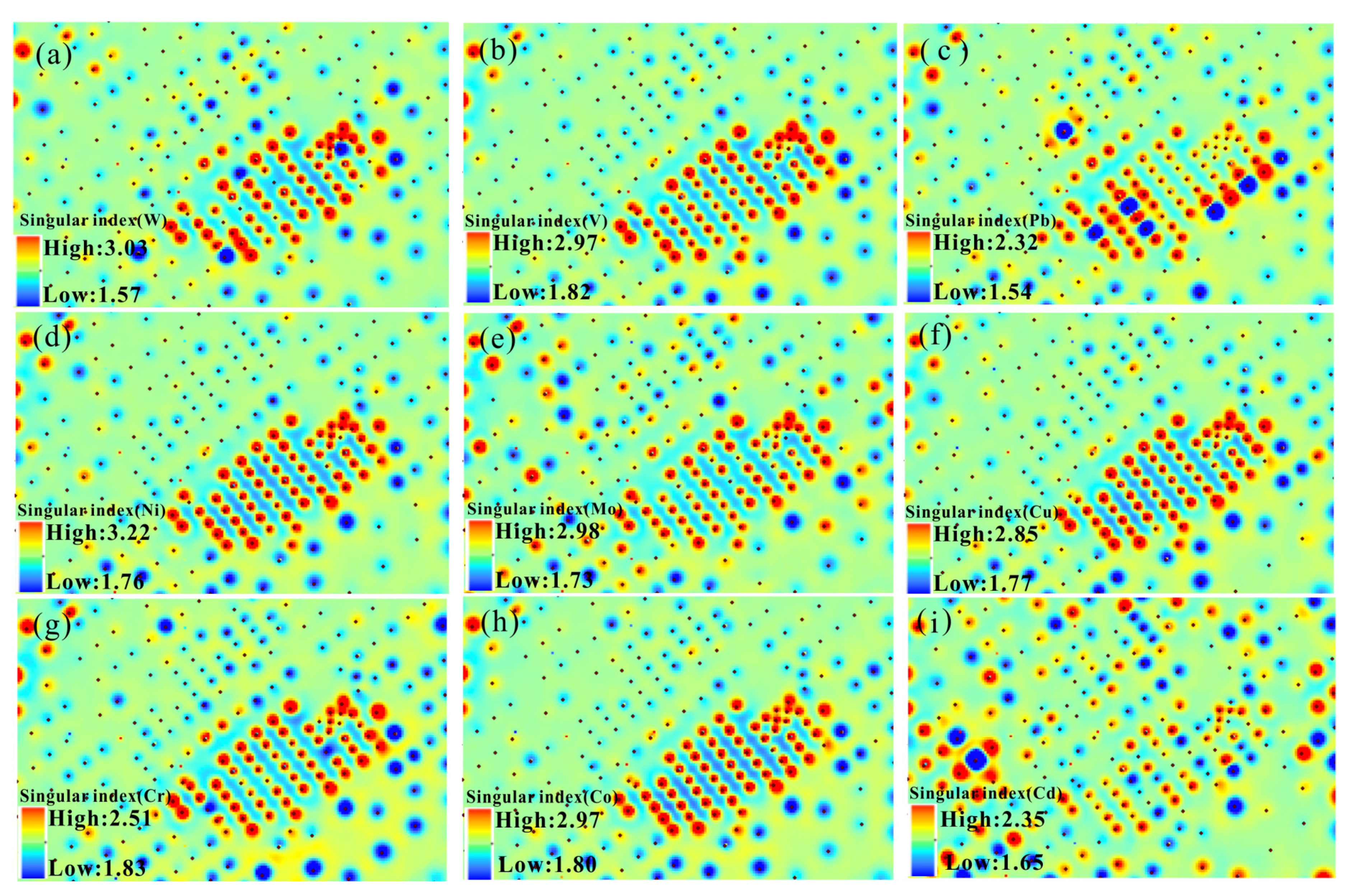
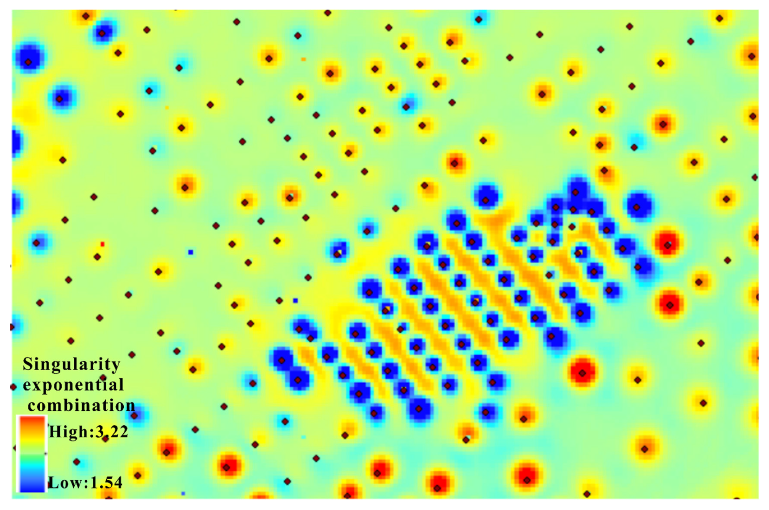
5.2. Local Singularity Analysis and Combined Local Anomaly Delineation

The present study performed PCA on the singular values of elements W, V, Pb, Ni, Mo, Cu, Cr, Co, and Cd (Figure 5) to delineate anomalies. The first PC of nine in total had the largest eigenvalue, accounting for ~70.5% of observed variance, and was composed of W, V, Pb, Ni, Mo, Cu, Cr, Co, and Cd. The comprehensive local singularity map formed by this combination of elements clearly reflected the spatial anomaly in local singularities in the Zhongsha area.

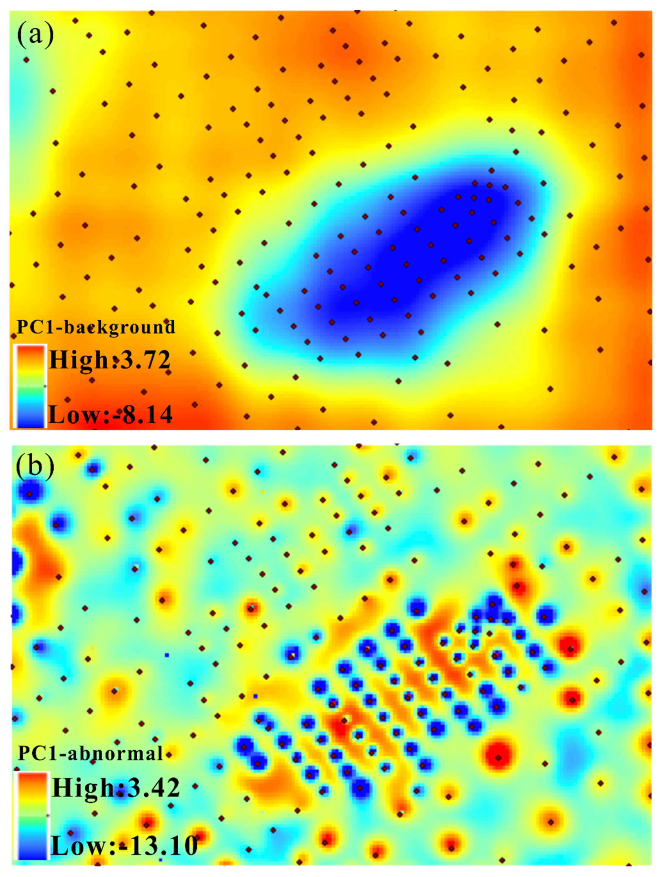
5.3. Decomposition and Delineation of Compound Anomalies

PCA was used to analyze data for W, V, Pb, Ni, Mo, Cu, Cr, Co, and Cd in the Zhongsha area. Since the distributions of these elements showed multifractal characteristics, logarithmic transformation of the original data was conducted before applying PCA. Figure 6a shows the characteristic distribution diagram calculated by PCA, whereas Figure 6b shows the load diagram of the first PC, which reflects the common contribution of all nine elements. Figure 7 shows the score diagram of the first PC.

The S-A method was used to transform the combined element anomaly diagram (Figure 7a) into a frequency domain by using Fourier transform to form the phase distribution diagram and the power spectrum distribution diagram, respectively. The relationship between the energy spectrum density (S) and the cumulative area was then plotted on the double logarithm diagram (Figure 7b). The relationship between the energy spectral density (S) and the cumulative area (A(≥S)) can be fitted by the least-squares method with two straight-line segments to form two value ranges of the energy spectral density S, which are separated by the threshold S = 1906. The relationship between energy spectral density and area in the first value range was log[A(≥S)] = 16.09S^−1.46. The standard error of the fitted result was 0.002, and the relationship between energy spectral density and area in the second value range was log[A(≥S)] = 13.41S^−1.12. The standard error of fitting was 0.007. Two filters can be constructed using the above two value ranges [32]: (1) the energy spectrum range with an energy spectrum density <1906, referred to as the “anomaly filter”; (2) the energy spectrum range with an energy spectrum density >1906, referred to as the “background filter”. Both the anomaly and background filters have irregular shapes. The two filters maintain the anisotropy of the corresponding geochemical fields and the internal structure in the two-dimensional energy spectrum space. The energy spectrum density and area in the corresponding energy spectrum interval of each filter obey the power-law distribution (fractal distribution). In other words, the energy spectrum density distributions in the two intervals have self-similarity.

The above anomaly and background filters can be used to decompose the original geochemical map into a background map and anomaly map (Figure 8a,b, respectively). The background map reflected the difference between the Zhongsha Plateau area and the surrounding area, whereas the heavy metal anomaly map showed where the metals were most concentrated in the deep sea plain. These maps can inform priority areas for the implementation of environmental pollution control measures.

6. Conclusions

The present study conducted the processing of geochemical data and delineation of anomalies in heavy metal concentrations in the surface sediments of the Zhongsha sea area using nonlinear theory. The current study introduced the application of the local singularity analysis method and generalized self-similarity analysis for the Zhongsha area. The spatial distributions of the local singularity index values for various heavy metals were first calculated, following which the composite anomalies were decomposed using the generalized self-similarity method. Future research on heavy metals in the Zhongsha region may benefit from the local anomalies discovered in the present study. The combined anomalies of the heavy metals W, V, Pb, Ni, Mo, Cu, Cr, Co, and Cd were delineated using local singularity analysis and the S-A generalized self-similarity anomaly decomposition method, combined with spatial PCA. Several combined anomalies in unknown regions are delineated by the heavy metal anomalies in the research area, which also represent the distribution of places with known high concentrations of heavy metals. Although these anomalies display different intensities and sizes and occur in different locations, they show self-similarity in the frequency domain and the characteristics of fractal density. In other words, the seemingly different anomalies evident in the geochemical maps for various heavy metals in the Zhongsha area can show self-similarity and comparability in the frequency domain.

References

- Wang, S.; Wang, S.; Liu, Y.; Wu, S. Tectonics and sedimentation of the Zhongsha trough basin: Implication to the basin evolution in distal rifting margin [J/OL]. Earth Sci. 2022, 47, 1094–1106. [Google Scholar]
- Chen, J.; Liu, S.; Wang, S.; Zhang, H.; Qin, Y.; Chen, W.; Wu, S. Characteristics and mechanism of the development of gravity flow deposits in Zhongsha Trough. Acta Sci. Nat. Univ. Sunyatseni 2022, 61, 39–54. [Google Scholar]
- Li, Y.; Huang, H.; Qiu, X.; Du, F.; Long, G.; Zhang, H.; Chen, H.; Wang, Q. Wide-angle and multi-channel seismic surveys in Zhongsha waters. Chin. J. Geophys. 2020, 63, 1523–1537. [Google Scholar]
- Zhao, B.; Gao, H.; Zhang, H.; Li, L. Structure study of the northeastern Zhongsha Trough Basin in the South China Sea based on prestack depth migration seismic imaging. J. Trop. Oceanogr. 2019, 38, 95–102. [Google Scholar]
- Yan, Q.; Shi, X.; Wang, K. Mineral provinces and matter source in surface sediments near the Zhongsha Islands in the South China Sea. Acta Oceanol. Sin. 2007, 29, 97–104. [Google Scholar]
- Yan, Q.; Wang, K.; Shi, X. Provinces and provenance of heavy minerals in surface sediments of the sea area near Zhongsha Islands in South China Sea. Mar. Geol. Quat. Geol. 2008, 28, 17–24. [Google Scholar]
- Zhang, J.; Peng, X.; Zhang, Y.; Wang, Y. Distribution of carbonate content in surface sediment from north of Zhongsha Islands to Northern slope in the South China Sea. Trop. Geogr. 2011, 31, 125–132. [Google Scholar]
- Wang, L.; Yu, K.; Wang, Y.; Wang, S.; Huang, X.; Zhang, R.; Wang, L. Distribution characteristic of heavy metals in coral reefs located in the Zhongsha Islands and Xisha Islands of South China Sea. Trop. Geogr. 2017, 37, 718–727. [Google Scholar]
- Michelutti, N.; Simonetti, A.; Briner, J.P.; Funder, S.; Creaser, R.A.; Wolfe, A.P. Temporal trends of pollution Pb and other metals in east-central Baffin Island inferred from lake sediment geochemistry. Sci. Total Environ. 2009, 407, 5653–5662. [Google Scholar] [CrossRef]
- Zhang, W.; Feng, H.; Chang, J.; Qu, J.; Xie, H.; Yu, L. Heavy metal contamination in surface sediments of Yangtze River intertidal zone: An assessment from different indexes. Environ. Pollut. 2009, 157, 1533–1543. [Google Scholar] [CrossRef]
- Hayaty, M.; Tavakoli Mohammadi, M.R.; Rezaei, A.; Shayestehfar, M.R. Risk Assessment and Ranking of Metals Using FDAHP and TOPSIS. Mine Water Environ. 2014, 33, 157–164. [Google Scholar] [CrossRef]
- Çevik, F.; Münir, Z.L.G.; Osman, B.D.; Fındık, Ö. An assessment of metal pollution in surface sediments of Seyhan dam by using enrichment factor, geoaccumulation index and statistical analyses. Environ. Monit. Assess. 2009, 152, 309–317. [Google Scholar] [CrossRef] [PubMed]
- Fu, F.; Wang, Q. Removal of heavy metal ions from waste waters: A review. J. Environ. Manag. 2011, 92, 407–418. [Google Scholar] [CrossRef]
- Rodríguez, L.; Ruiz, E.; Alonso-Azcárate, J.; Rincón, J. Heavy metal distribution and chemical speciation in tailings and soils around a Pb-Zn mine in Spain. J. Environ. Manag. 2009, 90, 1106–1116. [Google Scholar] [CrossRef]
- Christophoridis, C.; Dedepsidis, D.; Fytianos, K. Occurrence and distribution of selected heavy metals in the surface sediments of Thermaikos Gulf, N. Greece: Assessment using pollution indicators. J. Hazard. Mater. 2009, 168, 1082–1091. [Google Scholar] [CrossRef] [PubMed]
- Fang, H.; Chen, M.; Chen, Z. Environmental Characteristics and Models of Surface Sediments; Beijing Science Press: Beijing, China, 2009; pp. 1–3. [Google Scholar]
- Ali, R.; Hossein, H.; Seyedeh, B.F.M.; Sara, H.; Nima, J. Assessment of Heavy Metals Contamination in Surface Soils in Meiduk Copper Mine Area, SE Iran. Earth Sci. Malays. 2019, 3, 1–8. [Google Scholar]
- Ali, R.; Hossein, H.; Seyedeh, B.F.M.; Nima, J. Evaluation Of Heavy Metals Concentration In Jajarm Bauxite Deposit In Northeast Of Iran Using Environmental Pollution Indices. Malays. J. Geosci. 2019, 3, 12–20. [Google Scholar] [CrossRef]
- Limpert, E.; Stahel, W.A.; Abbt, M. Lognormal distributions across the sciences: Keys and clues. Bioscience 2001, 51, 341–352. [Google Scholar] [CrossRef]
- Xie, S.; Cheng, Q.; Xing, X.; Bao, Z.; Chen, Z. Geochemical multifractal distribution patterns in sediments from ordered streams. Geoderma 2010, 160, 36–46. [Google Scholar] [CrossRef]
- Zuo, R.; Wang, J. ArcFractal: An ArcGIS Add-In for Processing Geoscience Data Using Fractal/Multifractal Models. Nat. Resour. Res. 2020, 29, 3–12. [Google Scholar] [CrossRef]
- Buccione, R.; Mongelli, G.; Sinisi, R.; Boni, M. Relationship between geometric parameters and compositional data: A new approach to karst bauxites exploration. J. Geochem. Explor. 2016, 169, 192–201. [Google Scholar] [CrossRef]
- Xie, S.; Bao, Z. Fractal and multifractal properties of geochemical fields. Math. Geol. 2004, 36, 847–864. [Google Scholar] [CrossRef]
- Agterberg, F. Mixtures of multiplicative cascade models in geochemistry. Nonlinear Process. Geophys. 2007, 14, 201–209. [Google Scholar] [CrossRef]
- Cheng, Q.; Agterberg, F.; Ballantyne, S. The separation of geochemical anomalies from background by fractal methods. J. Geochem. Explor. 1994, 51, 109–130. [Google Scholar] [CrossRef]
- Huang, J. Features of the Zhongsha Atoll in the South China Sea. Mar. Geol. Quat. Geol. 1987, 7, 23–26. [Google Scholar]
- Cheng, Q. Multifractality and spatial statistics. Comput. Geosci. 1999, 25, 949–961. [Google Scholar] [CrossRef]
- Carranza, E.J.M.; Hale, M. Wildcat mapping of gold potential, Baguio district, Philippines. Trans. Inst. Min. Metall. B Appl. Earth Sci. 2002, 111, B100–B105. [Google Scholar] [CrossRef]
- Carranza, E.J.M. Improved wildcat modelling of mineral prospectivity. Resour. Geol. 2010, 60, 129–149. [Google Scholar] [CrossRef]
- Cheng, Q.; Bonham-Carter, G.; Wang, W.; Zhang, S.; Li, W.; Xia, Q. A spatially weighted principal component analysis for multi-element geochemical data for mapping locations of felsic intrusions in the Gejiu mineral district of Yunnan, China. Comput. Geosci. 2011, 37, 662–669. [Google Scholar] [CrossRef]
- Zhang, L.; Wang, G.; Yao, D.; Duan, G. Research and environmental significance of heavy metal in offshore sediment. Mar. Geol. Lett. 2003, 19, 6–9. [Google Scholar]
- Cheng, Q.; Zhao, P.; Chen, J.; Xia, Q.; Chen, Z.; Zhang, S.; Xu, D.; Xie, S.; Wang, W. Application of Singularity Theory in Prediction of Tin and Copper Mineral Deposits in Gejiu District, Yunnan, China: Weak Information Extraction and Mixing Information Decomposition. Earth Sci.-J. China Univ. Geosci. 2009, 34, 232–242. [Google Scholar]
- Cicchella, D.; De Vivo, B.; Lima, A.; Albanese, S.; McGill, R.A.R.; Parrish, R.R. Heavy metal pollution and Pb isotopes in urban soils of Napoli. Ital. Geochemistry: Exploration, Environment. Analysis 2008, 8, 103–112. [Google Scholar]
Publisher’s Note: MDPI stays neutral with regard to jurisdictional claims in published maps and institutional affiliations. |
© 2022 by the authors. Licensee MDPI, Basel, Switzerland. This article is an open access article distributed under the terms and conditions of the Creative Commons Attribution (CC BY) license (https://creativecommons.org/licenses/by/4.0/).
Share and Cite
Zhang, Y.; Liu, S.; Zhang, L.; Zhou, Y.; Liang, J.; Lu, J.; Hu, X.; Liu, L.; Chen, L.; Zhang, J.; et al. Application of Singularity Theory to the Distribution of Heavy Metals in Surface Sediments of the Zhongsha Islands. J. Mar. Sci. Eng. 2022, 10, 1697. https://doi.org/10.3390/jmse10111697
Zhang Y, Liu S, Zhang L, Zhou Y, Liang J, Lu J, Hu X, Liu L, Chen L, Zhang J, et al. Application of Singularity Theory to the Distribution of Heavy Metals in Surface Sediments of the Zhongsha Islands. Journal of Marine Science and Engineering. 2022; 10(11):1697. https://doi.org/10.3390/jmse10111697
Chicago/Turabian StyleZhang, Yan, Shiqiao Liu, Li Zhang, Yongzhang Zhou, Jinqiang Liang, Jing’an Lu, Xiaoqiang Hu, Liang Liu, Liang Chen, Jingwei Zhang, and et al. 2022. "Application of Singularity Theory to the Distribution of Heavy Metals in Surface Sediments of the Zhongsha Islands" Journal of Marine Science and Engineering 10, no. 11: 1697. https://doi.org/10.3390/jmse10111697
APA StyleZhang, Y., Liu, S., Zhang, L., Zhou, Y., Liang, J., Lu, J., Hu, X., Liu, L., Chen, L., Zhang, J., Xu, C., & Dong, X. (2022). Application of Singularity Theory to the Distribution of Heavy Metals in Surface Sediments of the Zhongsha Islands. Journal of Marine Science and Engineering, 10(11), 1697. https://doi.org/10.3390/jmse10111697