Path Planning of Multi-Objective Underwater Robot Based on Improved Sparrow Search Algorithm in Complex Marine Environment

Abstract

Autonomous underwater vehicle (AUV) path planning in complex marine environments meets many chanllenges, such as many influencing factors, complex models and the performance of the optimization algorithm to be improved. To find a path with minimum cost of the actual environmental threats, navigation height changes and the minimum energy consumption of the AUV, an improved sparrow search algorithm is designed under the impact of the time-varying characteristics of the current in the complex marine environment on the AUV and the physical constraints of the AUV movement. In the proposed algorithm, an adaptive weight factor balance strategy is introduced into the position update of the discoverer to improve the convergence speed and search ability. In the follower position, the variable spiral search strategy is improved based on the position update formula to enhance the local jumping ability of the algorithm. After the position update, Levy flying strategy is added, and Cauchy–Gaussian mutation is performed on the optimal individual to increase the population diversity, which improves the anti-stagnation ability of the algorithm. Finally, the AUV global path with minimum cost in the sense of multi-objective weighting is obtained. The simulation results show that the proposed algorithm can plan a path with less cost and quickly converge to an optimized point, and finally it can meet the global path planning requirements of AUV when navigating in complex sea areas.

1. Introduction

In recent years, marine exploration and exploitation have received increasing attention as the demand for marine resource exploration and data collection has increased, and marine resources have shown great value [1]. As an important part of underwater survey, autonomous underwater vehicle (AUV) have been widely applied in scientific research, military and civil fields due to their energy, high autonomy, high flexibility and wide detection range [2,3,4]. AUV research, manufacturing technology, sensors, computing power and battery technology have been continuously developed. A reliable and fully automatic decision-making robot system is the current goal of AUV research [5]. However, in the complex marine environment, how to perform efficient path planning of AUV is an important key technology.

There are many commonly used global path planning methods in AUV path planning, including traditional and intelligent path planning. The traditional AUV path planning methods include the A* algorithm [6], D* algorithm [7] and artificial potential field method [8], etc. The intelligent AUV path planning methods include the particle swarm algorithm [9], ant colony algorithm [10], genetic algorithm [11] and path planning method based on machine learning [12], etc. On this basis, researchers continue to propose new path planning methods or improve and fuse previous algorithms. Zhang et al. [13] proposed an improved particle swarm optimization algorithm for the global path planning problem of AUV in the sea area with complex conditions, but this method only considered the prior environmental information and did not consider the dynamic environmental model. Yin et al. [14] proposed an imperial competition for AUV path planning in static terrain obstacles and irregular current environments. Still, they did not consider the real seabed environment and time-varying current information. Cao et al. [15] proposed a velocity vector synthesis method combined with a belief function method to overcome the influence of current on AUV navigation. Although the method considered the influence of time-varying ocean current, it did not consider the real terrain and multiple constraints.

However, most of the above studies ignore the effects of time-varying ocean current, real terrain and multiple constraints on AUV navigation. These impacts often directly affect AUV navigation; for example, strong ocean current will threaten AUV navigation safety, but reasonable use of ocean current energy can save AUV energy consumption [16]. On this basis, this paper considers the effect of time-varying current characteristics on navigation and takes the actual environmental threat, the change in navigation altitude and minimum AUV energy consumption as the path planning objectives under the physical constraints of AUV motion. An improved sparrow search algorithm is designed to obtain the global path of the AUV with minimum cost in a multi-objective weighted sense.

2. Modeling Multi-Objective AUV Path Planning Problems in Complex Ocean Environments

Real terrain, the time-varying current model, potential threats and physical constraints of the AUV should be considered when the AUV performs its mission in complex oceanic environments. From this perspective, a comprehensive cost function for AUV navigation is established in terms of topography, sailing altitude change, energy consumption under time-varying currents, underwater threats, physical constraints, etc. Suppose a complete route has $n$ nodes, where the coordinates of the $i$th navigational trajectory point are denoted (X_i, Y_i, Z_i) noted as $g_i$. This paper considers that the physical constraint is that the turning angle does not exceed 90°. The terrain constraint means that the planned path point needs to be higher than the terrain. The total cost function is as follows:

$$\min F={\omega }_1{f}_H+{\omega }_2{f}_T+{\omega }_3{f}_E$$

(1)

$$s.t.{\displaystyle \sum _{i=1}^3{\omega }_i=1}$$

(2)

$${\alpha }_{\max }\le {90}^{°}$$

(3)

$$z_i-h_i\ge 0$$

(4)

where ${\omega }_i$ is the weight coefficient; ${\alpha }_{\max }$ is the maximum turning angle; $z_i$ is the vertical height of the $i$th track point from the seafloor; $h_i$ is the terrain elevation value corresponding to the $i$th track point; $f_H$, $f_T$ and $f_E$ are the height cost [17], threat cost [18] and energy cost [19], respectively; Equations (2)–(4) are the weight coefficient constraint, maximum turning angle constraint and terrain constraint, respectively. The respective costs are as follows:

$$\{\begin{array}{c}{f}_H=\sqrt{\frac{1}{n}{\displaystyle \sum _{i=0}^{n-1}{(z_i-\overline{z})}^2}}\\ \overline{z}=\frac{1}{n}{\displaystyle \sum _{i=0}^{n-1}{z}_i }\end{array}$$

(5)

where $f_H$ is the standard deviation cost function of the navigational altitude, and $\overline{z}$ is the mean of the sailing altitude. Reference [15] mentioned that the navigation height should not change too much, and a stable navigation height can reduce the burden of the control system and save more energy.

$$f_T=\{\begin{array}{cc}{\displaystyle \sum _{i=0}^{n-1}\frac{K_T}{{(d_{ij})}^4}},\hfill & d_{ij}<R_{Tj}\\ 0,\hfill & d_{ij}>R_{Tj}\end{array}$$

(6)

where $K_T$ is the threat coefficient; $d_{ij}$ is the straight-line distance from the $i$th trajectory point to the center $j$ of the spherical obstacle or threat area; $R_{Tj}$ is the radius of the spherical obstacle or the radius of the threat area.

$$\{\begin{array}{c}{f}_E={\displaystyle \sum _{i=0}^{n-1}k·|V_e{|}^3·\frac{\left|\stackrel{\rightharpoonup }{g_i{g}_{i+1}}\right|}{\left|V\right|}}\\ V=\left|V_e+V_c\cos (V_e,V_c)\right|\end{array}$$

(7)

where $k$ is the drag coefficient, the value of which is determined by the AUV design and is taken as 3.425 in this paper based on experience; $\left|\overrightarrow{g_i{g}_{i+1}}\right|$ is the modulo value of the path point $g_i$ to $g_{i+1}$ vector; $V$ is the real speed; $V_e$ is the desired speed, which is taken as 2.5 m/s; $V_c$ is the time-varying seawater velocity, which can be obtained from the time-varying ocean current equation in the literature [20]. The literature only considers the cost of AUV sailing time and does not comprehensively consider other costs during sailing. $\cos (V_e,V_c)$ is the cosine of the angle between the desired speed and the seawater flow velocity vector.

3. An Improved Sparrow Search Algorithm

The sparrow search algorithm (SSA) is an optimization algorithm proposed by imitating the group foraging behavior of sparrows [21]. The main difference between this algorithm and the traditional group algorithm is that the population is divided into three categories: discoverers, followers and vigilantes. There is also an early warning mechanism. The discoverer generally has a good fitness value and is responsible for providing discovery for other individuals in the entire population to obtain food; the follower improves fitness by following the discoverers for food; the vigilant are predators that watch their surroundings for companions and threats, and sparrows that sense danger will sound an alarm to warn their companions away from it. In the process of foraging, the positions of the three will be constantly updated to obtain the optimal food source, and the position of the optimal food source is the optimal solution. To improve the optimization performance of the sparrow algorithm and improve the algorithm’s shortcomings, the following focuses on the improvement strategy of the sparrow algorithm.

3.1. Discoverer Adaptive Adjustment Strategy

The discoverer adopts a random search strategy in the foraging process, and this strategy slows down the convergence rate to some extent. Inspired by [22], this paper introduces adaptive inertial weights into the discoverer’s update equation, which are described mathematically as follows:

$$X_{i,j}^{t+1}=\{\begin{array}{cc}{X}_{i,j}^t·\exp (-\frac{\omega ·i}{\alpha ·ite{r}_{\max }})\hfill & if R_2<ST\hfill \\ X_{i,j}^t+Q·L\hfill & if R_2\ge ST\hfill \end{array}$$

(8)

$$\omega =a\times {\left(1-{\left(\frac{t}{Ite{r}_{\max }}\right)}^{\eta }\right)}^{1/\eta }$$

(9)

where $X_{i,j}$ is defined as the position of the $i$th sparrow in the $j$th dimension; $t$ is the current iteration number; $R_2$ is a random number from 0 to 1; $ST\in [0.5,1]$, which is taken as 0.5 in this paper; $Q$ is a random number that obeys a normal distribution; $L$ represents a 1 × d matrix, where each element in the matrix is 1; $Ite{r}_{\max }$ is the maximum iteration number; $a$ is a constant, which is set to 1 in this paper; $\eta$ is the step size adjustment coefficient, which is taken as 1.2 in this paper. $\omega$ is an adaptive inertial weight, and the value of $\omega$ decreases with the number of iterations. At the beginning of the iteration, the $\omega$ value is larger, corresponding to a wider range of sparrows preying. However, the $\omega$ value of the later iterations is small, which is beneficial to the algorithm’s convergence.

3.2. Follower Variable Spiral Search Strategy

In the SSA, the follower follows the discoverer’s lead and performs a detailed search around it. One can see that the discoverer has stronger global exploration ability, while the follower is better at local development. This also leads to an insufficient search range for followers, and it is easy to fall into local optimum, resulting in reduced accuracy.

Inspired by the helical flight of moths [23], this paper introduces a variable helical position update strategy, which enables the follower to have multiple search paths to update the position better while balancing the global and local search of the algorithm. After integrating the spiral strategy, the participants explore the search space in the form of a spiral, which increases the ability of the participants to explore unknown areas, then increases the possibility of the algorithm jumping out of the local optimum and is conducive to improving the global search performance of the algorithm.

The improved follower position update is as follows:

$$X_{i,j}^{t+1}=\{\begin{array}{cc}{e}^{zl}·\cos (2\pi l)·Q·\exp (\frac{X_{worst}-X_{i,j}^t}{i^2})\hfill & if i>n/2\hfill \\ X_p^{t+1}+|X_{i,j}^t-X_p^{t+1}|·A^{+}·L·e^{zl}·\cos (2\pi l) \hfill & otherwise\hfill \end{array}$$

(10)

$$z=e^{k\times \cos (\pi \times (1-(t/Ite{r}_{\max })))}$$

(11)

where $z$ varies according to the number of iterations; $k$ is the coefficient of variation taken as 5 in this paper; $l$ is a random number within [−1,1]. $X_P$ is the current best position occupied by the finder, and $X_{worst}$ represents the global worst position in the current sparrow population. $A$ denotes a $1\times d$ matrix where each element is randomly assigned a value of 1 or −1, and $A^{+}=A^T{(A{A}^T)}^{-1}$.

3.3. Levy Flight Strategy

This paper adds the random walk generated by the Levy flight strategy into sparrow updating. After the discoverers and followers complete the position update, the sparrow individuals satisfying the condition of Equation (12) are updated by the Levy flight strategy. The uncertainty in Levy’s direction of flight and step length reinforces the diversification of search directions, which improves the diversity of population positions and avoids falling into the local optimum. The random Levy flight step size [24] can be obtained by the following equation:

$$X_i^{t+1}=\{\begin{array}{cc}{X}_i^t+L·(X_i^t-X_{best}),& if rand(1)>P\&f(X_i^{t+1})<f(X_i^t)\hfill \\ X_i^t& \mathrm{otherwise}\hfill \end{array}$$

(12)

$$\{\begin{array}{l}\begin{array}{l}P=(1-t/Ite{r}_{\max })\\ L=\mu /{\left|v\right|}^{1/\beta },\beta =3/2\end{array}\hfill \\ \mu ~N\left(0,{\sigma }_{\mu }^2\right),v~N\left(0,{\sigma }_v^2\right)\hfill \\ {\sigma }_{\mu }={\left\{\frac{\Gamma (1+\beta )\sin (\pi \beta /2)}{\beta ·\Gamma [(1+\beta )/2]·2^{(\beta -1)/2}}\right\}}^{1/\beta },{\sigma }_v=1\hfill \end{array}$$

(13)

where $X_{best}$ is the position representing the current global optimum, $f(X_i^t)$ is the fitness value of the current sparrow individual, and $f(X_i^{t+1})$ is the fitness value after the revised Levy flight strategy. If the v fitness value is smaller than the current fitness value, then update the position according to the Levy flight strategy; otherwise, it will not be updated. $L$ is the Levy flight path, $\mu$ and $v$ are random numbers that follow the normal distribution, $\mu ~N(0,{\sigma }_{\mu }^2)$, $v~N(0,{\sigma }_v^2)$, the range of the parameter $\beta$ takes the value $0<\beta <2$, and generally, $\beta =1.5$.

3.4. Cauchy–Gaussian Mutation Strategy

In the foraging process, sparrows gradually move closer to the optimal individuals, resulting in insufficient population diversity, and the algorithm easily falls into local optimality. To solve this problem, this paper introduces the Cauchy–Gaussian mutation strategy [25], which mutates the individuals with the current optimal fitness to improve their global foraging ability. The mathematical description of the mutation strategy is as follows:

$$U_{best}^{t+1}=X_{best}^t[1+{\lambda }_{1}cauhy(0,{\sigma }^2)+{\lambda }_{1}Gauss(0,{\sigma }^2)]$$

(14)

$$\sigma =\{\begin{array}{c}1, f(X_{best})<f(X_i)\\ \exp (\frac{f(X_{best})-f(X_i)}{|f(X_{best})|}), otherwise\end{array}$$

(15)

where $U_{best}^{t+1}$ denotes the position of the optimal individual after mutation; ${\sigma }^2$ denotes the standard deviation of the Cauchy–Gaussian mutation; $Gauhy(0,{\sigma }^2)$ is a random variable satisfying the Cauchy distribution; $Gauss(0,{\sigma }^2)$ is a random variable satisfying the Gaussian distribution; ${\lambda }_1=1-t^2/{(Ite{r}_{\max })}^2$ and ${\lambda }_2=t^2/{(Ite{r}_{\max })}^2$ are dynamic parameters that adjust adaptively with the number of iterations, with ${\lambda }_1$ gradually increasing and ${\lambda }_2$ gradually decreasing in the process of finding the optimal.

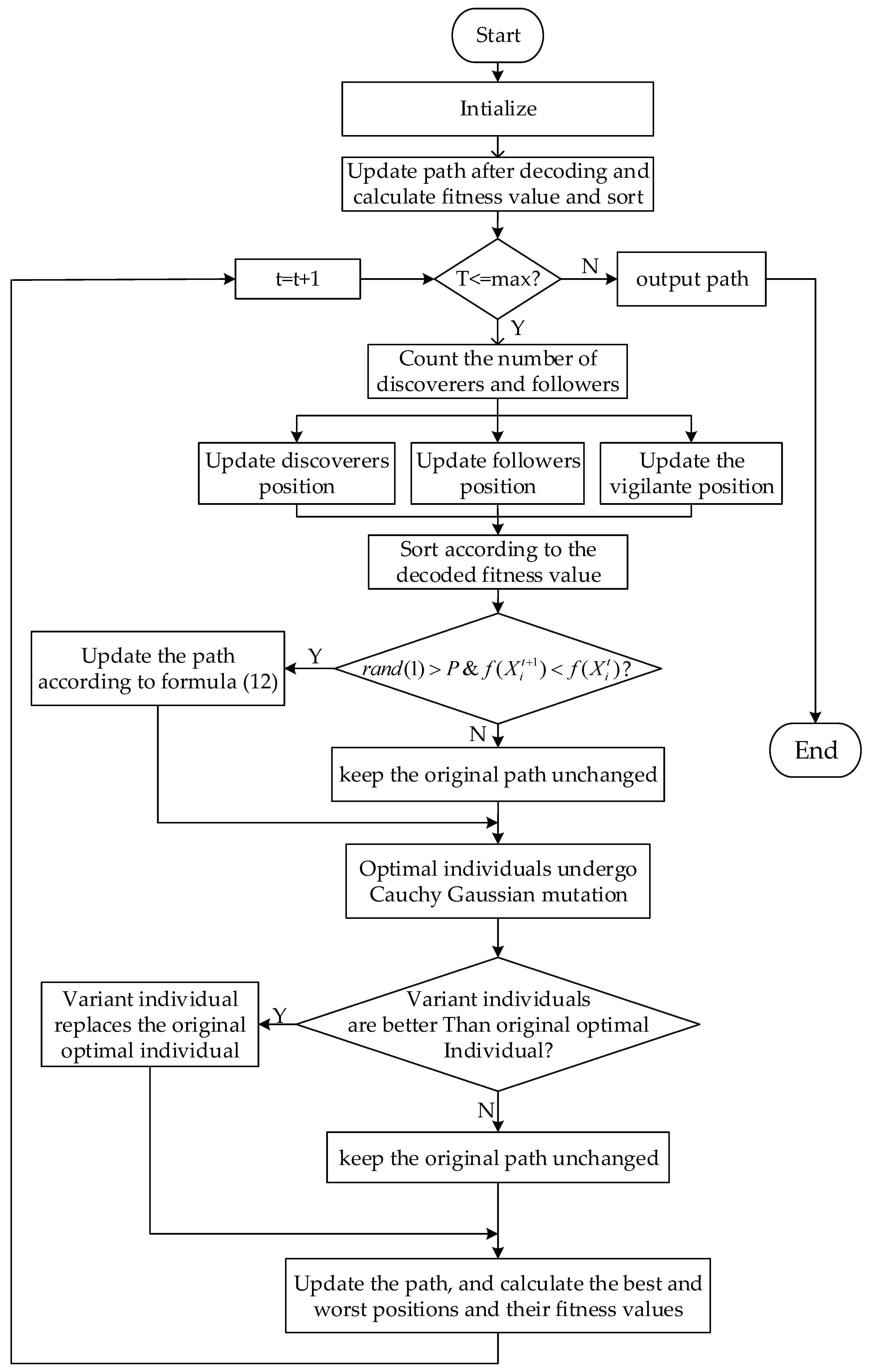
4. Method for AUV Path Planning Based on Improved SSA

4.1. Path Coding

When solving path planning problems using the sparrow search algorithm, each path is a line consisting of multiple trajectory points connected. A sparrow in the population is defined as a path $X_i=[X_{i,1},X_{i,2},\cdots X_{i,j}]$, and every three dimensions $X_{i,j}$ in the sparrow represent the coordinates of the trajectory points in the $x,y,z$ directions in turn, so there are $j/3$ navigation track points. In solving the AUV 3D path planning problem using the SSA, the number of track points $n$ is determined, and the optimal navigation route is determined by optimizing the $x$, $y$ and $z$ coordinates.

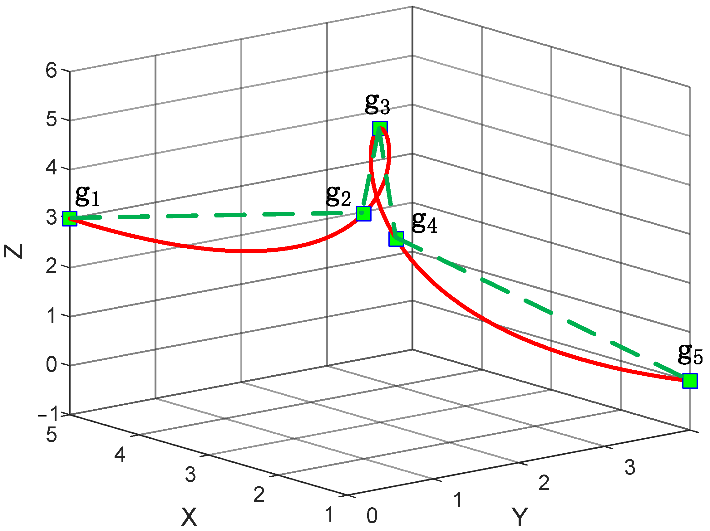
4.2. Decoding of Path Smoothing Based on B-Spline Interpolation

The AUV navigation trajectory is composed of line segments. To ensure the smooth turning of the path and avoid the physical constraints of the AUV, the B-spline curve is used to smooth the path. The method is characterized by overall global optimization, geometric invariance, continuity, symmetry, recursion, convexity preservation and microperformance [26]. Assuming that the AUV path is $g=(g_1,g_2,\cdots ,g_n)$, each path point $g_i(i=1,2,\cdots ,n)$ has three dimensions $(x,y,z)$, and the cubic spline interpolation is performed on $(x_1,x_2,\cdots ,x_n)$, $(y_1,y_2,\cdots ,y_n)$ and $(z_1,z_2,\cdots ,z_n)$, respectively, and finally, a smooth path is formed. The effect of cubic spline curve is shown in Figure 1. The green line segment is the original path, and the red curve is the smoothed path.

4.3. Improved SSA for AUV Path Planning

This section describes the calculation steps of path planning using the improved SSA. The pseudo-code of the algorithm is shown in Algorithm 1, and the flow chart is shown in Figure 2.

Algorithm 1: Improved SSA algorithm AUV path planning pseudo-code

/*Initialization*/

1. Set the maximum iterations as $Ite{r}_{\max }$;

2. Set the total number of sparrows as $M$;

3. Set the number of discoverers as $PD$;

4. Set the number of sparrows perceiving danger as $SD$;

5. Set the alarm value as $R_2$;

6. Set the start point $(x_S,{\mathrm{y}}_S,z_S)$, target point $(x_G,y_G,z_G)$, the boundaries of the map space and the number of control points $n$;

7. Set the position and range of threat areas and spherical obstacles, initialize the currents and initialize the sparrow population by the principle of trajectory coding;

/*Iterative search*/

8. While(t < $Ite{r}_{\max }$)

9. Each sparrow represents a path. After decoding the generated path, the cost is calculated using the cost function Equation (1), and then the sparrow population is sorted;

10. $R_2=rand(1)$;

11. for $i=1:PD$

12.        Update the discoverer’s position using Equation (8);

13. end for

14. for $i=(PD+1):M$

15.        Update the follower’s position using Equation (10);

16. end for

17. for $i=1:SD$

18.     Update the threatened sparrow’s position;

19. end for

20. for $i=1:M$

21.        if $rand(1)>P$

22.            if $f(X_i^{t+1})<f(X_i^t)$

23.                Update the sparrow position using Equation (12);

24.            end if

25.         end if

26. end for

27. Update the optimal sparrow position using Equation (14);

28. Get the current new path;

29. If the new path is better than before, update it;

30. $t=t+1$

31. end while

32. Output the best route and its cost value.

33. Post-processing and visualization

5. Simulation Experiment and Result Analysis

The simulation experiments were performed on a computer with a CPU of AMD Ryzen 7 5800H 3.5 GHz and 16 GB of RAM, operating system of Windows 10 and compiled software of Matlab R2020b. The topographic data in this paper were obtained from the Global Bathymetric Chart of Oceans (GEBCO) [27], and the latitude and longitude used are (Lng: 117.0000° W, Lat: 23.9099° N) and (Lng: 137.0000° W, Lat: 17.9099° N). Among them, the selected area is 100*100 km, the deepest point in the sea area is $Z=0$, and the depth of other positions is determined according to the difference from this point. The X-axis is the direction of increasing longitude, and the Y-axis is the direction of increasing latitude. To reduce the calculation and improve the map diversity, the range is compressed to 200 × 200 × 200 in scale. The reciprocal interpolation method is used to approximate the environmental information of the continuous space, and the three-dimensional underwater terrain is established. Figure 3 is the three-dimensional map creation diagram. Figure 3a is the GEBCO plug-in display diagram. The red square in the figure is the selected sea area box. Select the specified sea area box to download the corresponding sampling matrix for subsequent global path planning research. Figure 3b shows the established 3D static environment map.

The experimental part of this paper is divided into the offshore sea scene and the distant sea scene, in which there are cylindrical threats in the offshore sea scene and spherical obstacles in the distant sea scene. As shown in

Table 1. Position parameter settings in two sea area scenarios.

Terrain Scene	Start Point	Target Point	Center Point Coordinates	Action Radius(Units)
Offshore sea scene with cylindrical threat source	(15, 14, 80)	(172, 185, 80)	(150, 50), (50, 150), (40, 50), (150, 150), (120, 10), (110, 100)	10
Distant sea scene with spherical obstacles	(23, 174, 120)	(190, 10, 150)	(150, 40, 130), (50, 165, 110), (50, 110, 140), (150, 150, 110), (120, 10, 120), (110, 90, 150), (95, 55, 140), (40, 50, 130), (155, 65, 140)	10

, the coordinates of the starting point, end point, cylindrical threat source or spherical obstacle center of path planning in the two terrain scenarios, as well as their respective radius units are displayed.

There are five algorithms in the experiment, including the improved SSA, SSA, particle swarm optimization (PSO) [28], artificial bee colony (ABC) [29] and artificial fish swarm algorithm (AFSA) [30]. The PSO algorithm, ABC algorithm and AFSAS algorithm are standard original algorithms. All three algorithms are widely used in the field of 3D path planning and are therefore chosen for comparison. In this experiment, the parameters of all algorithms were set according to their respective references, and the population of each algorithm was set to 50, with a maximum number of 200 iterations. For the improved SSA and SSA, the number of discoverers is 20% of the total number of sparrows, the number of sparrows aware of the danger is 15% of the total, and the safety threshold is 0.8. Each algorithm is run independently 30 times, and the performance of each algorithm is evaluated and compared through the experimental results.

The simulation experiment in this paper is divided into two types of sea areas: Scenario 1: Distant Seas and Scenario 2: Offshore Seas. In the offshore sea area, there are usually defensive radar detection threat areas, so the threat cost of operating in this sea should focus on consideration. Meanwhile, the execution of distant sea operations often navigates a long distance, so the simulation under this condition should focus on the energy consumption cost. Therefore, in this paper, different coefficient weights are set in the two sea areas. Equation (1) is used as the cost in both scenarios, where

Table 2. The main parameters for Scenario 1.

Parameter	Symbol	Parameter Value
Threat source threat factor	$K_T$	10,000
Height constraint weights	${\omega }_1$	0.3
Threat source constraint weights	${\omega }_2$	0.4
Energy constraint weights	${\omega }_3$	0.3

is the main parameters of offshore sea and

Table 3. The main parameters for Scenario 2.

Parameter	Symbol	Parameter Value
Threat source threat factor	$K_T$	10,000
Height constraint weights	${\omega }_1$	0.2
Threat source constraint weights	${\omega }_2$	0.2
Energy constraint weights	${\omega }_3$	0.6

is the main parameters of distant sea.

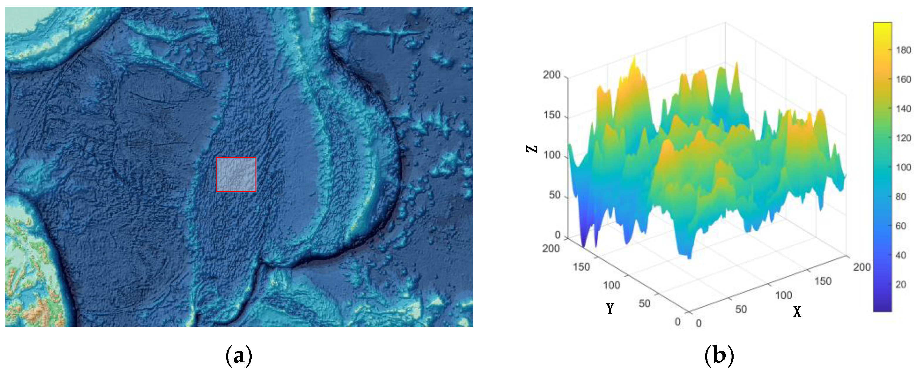
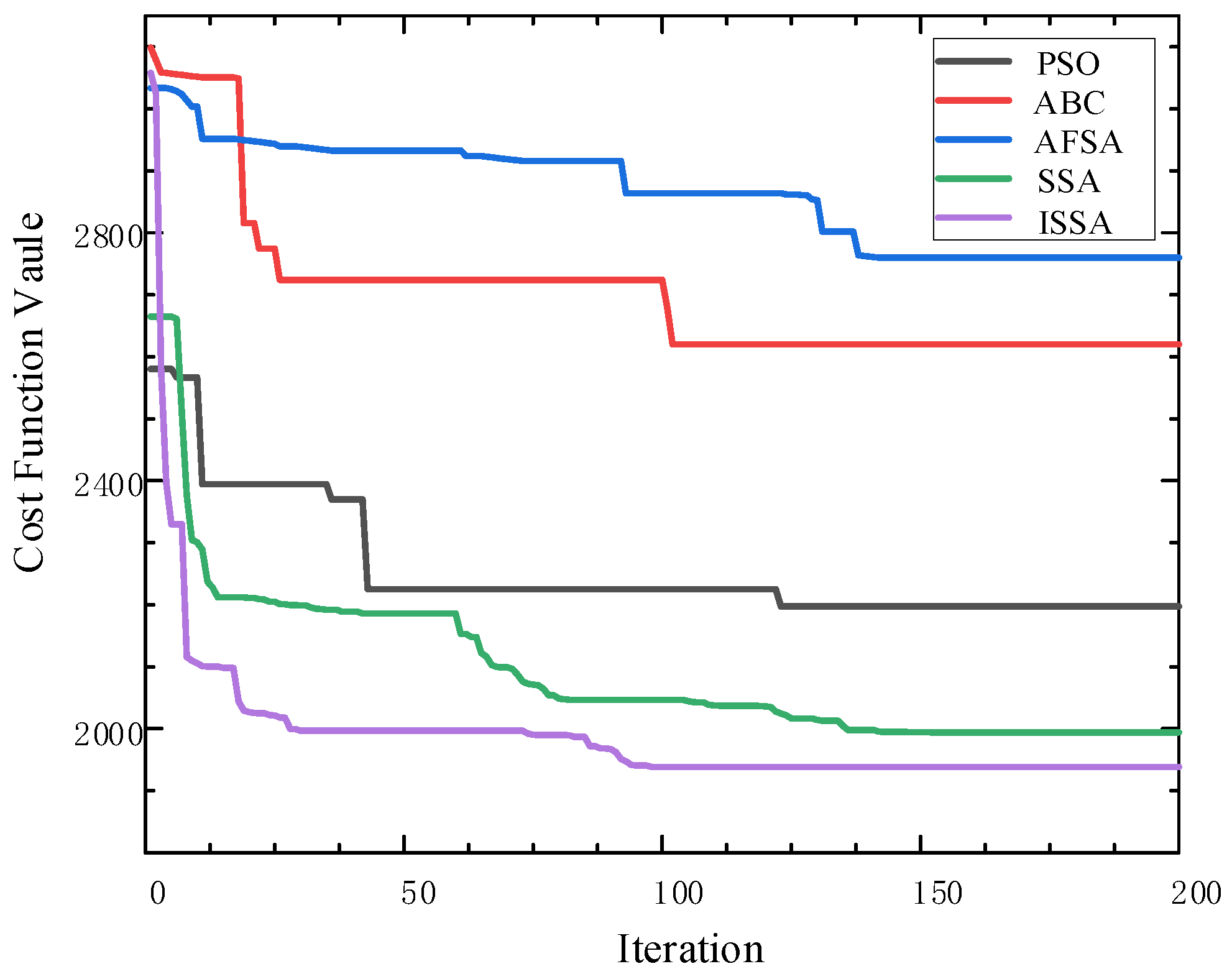
5.1. Comparison of Simulation Results in Offshore Sea Scenarios

The defensive-oriented offshore sea area is usually deployed with defensive radars to detect the threat area operation, and the blue columns are used to represent the inaccessible threat area for such a sea area. When the AUV accomplishes its mission in this terrain, avoiding such a dangerous area becomes one of the most important objectives.

Figure 4 shows the path trajectory of the improved SSA and the other four algorithms in the offshore sea scenario. Wherein, a and b are the route comparison map and side view in three-dimensional space, respectively, and c, d and e are potential field maps of current at T = 25, T = 50 and T = 80, respectively. The route in the figure is the plan of the AUV navigation path, the marked points are the navigation points corresponding to these moments, and the yellow circle represents the plane area of the threat area.

Table 4. Comparison of algorithms results in offshore sea scenarios.

Algorithm	Best Value	Worst Value	Average Value	Standard Deviation
PSO	1919.86	2933.71	2445.83	343.75
ABC	2161.51	3118.46	2660.74	243.80
AFSA	2489.44	3349.52	2873.51	323.69
SSA	1804.47	2099.64	1954.81	93.51
ISSA	1777.53	2020.13	1900.73	83.11

shows the comparison of algorithms for navigation results in the offshore area scenario.

Table 5. Comparison of error percentage of each algorithm in the offshore scene. (Improved SSA as benchmark.)

Algorithm	Best Value Error Percentage	Worst Value Error Percentage	Average Value Error Percentage
PSO	8.01%	45.22%	28.68%
ABC	21.60%	54.37%	39.99%
AFSA	40.05%	65.81%	51.18%
SSA	1.52%	3.94%	2.85%

is the comparison of cost error percentage, with the improved SSA as the benchmark. Figure 5 shows the cost curve of algorithms in the AUV offshore area scenario.

It can be seen from the above figure that in the offshore sea scene, the improved SSA can not only plan a collision-free path but also the average cost is better than that of the other four algorithms. From the side view of the route comparison in Figure 4b, it can be seen that the improved SSA plans out a smoother height change than the other four algorithms, so the corresponding height change constraint is smaller. At first, it can be seen from Figure 4c that in the early stage of planning, only the AFSA can use the ocean current to navigate, and the ocean current has little influence on the planning of the other four algorithms. Secondly, as the time increases to the T = 50 moment, as shown in Figure 4d, it can be seen that the paths planned by the improved SSA, PSO algorithm and ABC algorithm can better use the ocean current energy to navigate and reduce the navigation cost. Finally, in the later stage of the navigation, as shown in Figure 4e, with the improvement at time T = 80, compared with the other three algorithms, the paths generated by the improved SSA and the SSA can still make better use of the ocean current for navigation and reduce the navigation cost. Considering comprehensive AUV navigation at different moments, from the energy consumption constraint Equation (7), it can be seen that the improved SSA can use the ocean current navigation in the main navigation phase, and the navigation distance is shorter than that of other algorithms, so the energy consumption constraint is also smaller.

Table 4 shows that the values of the improved SSA are better than those of the other four algorithms in the offshore scene. The standard deviation of the first three algorithms is significant, and the standard deviation of the last two algorithms is small. This is because the environment is more complex, and the first three algorithms have to choose a longer route to meet the navigation conditions. The improved SSA performs better on this complex optimization problem because the performance of the sparrow algorithm itself is better than that of other algorithms, and our improvement strategy is effective. Table 5 is the comparison of cost error percentage, with the improved SSA as the benchmark. Refer to literature [31] for the calculation method of error percentage. It can be seen that the performance of the first three algorithms has a gap compared with the improved SSA. There is a small gap between the improved SSA and the SSA. This is because the two algorithms have essentially been close to the extreme value in the optimization process. The improved SSA is still better than the SSA in the extreme value range. It can be seen from the above figure and table that in the offshore sea area, the improved SSA has a smaller navigation altitude change cost and can make better use of ocean current energy to reduce the energy consumption cost. The global path cost is smaller than that of other algorithms.

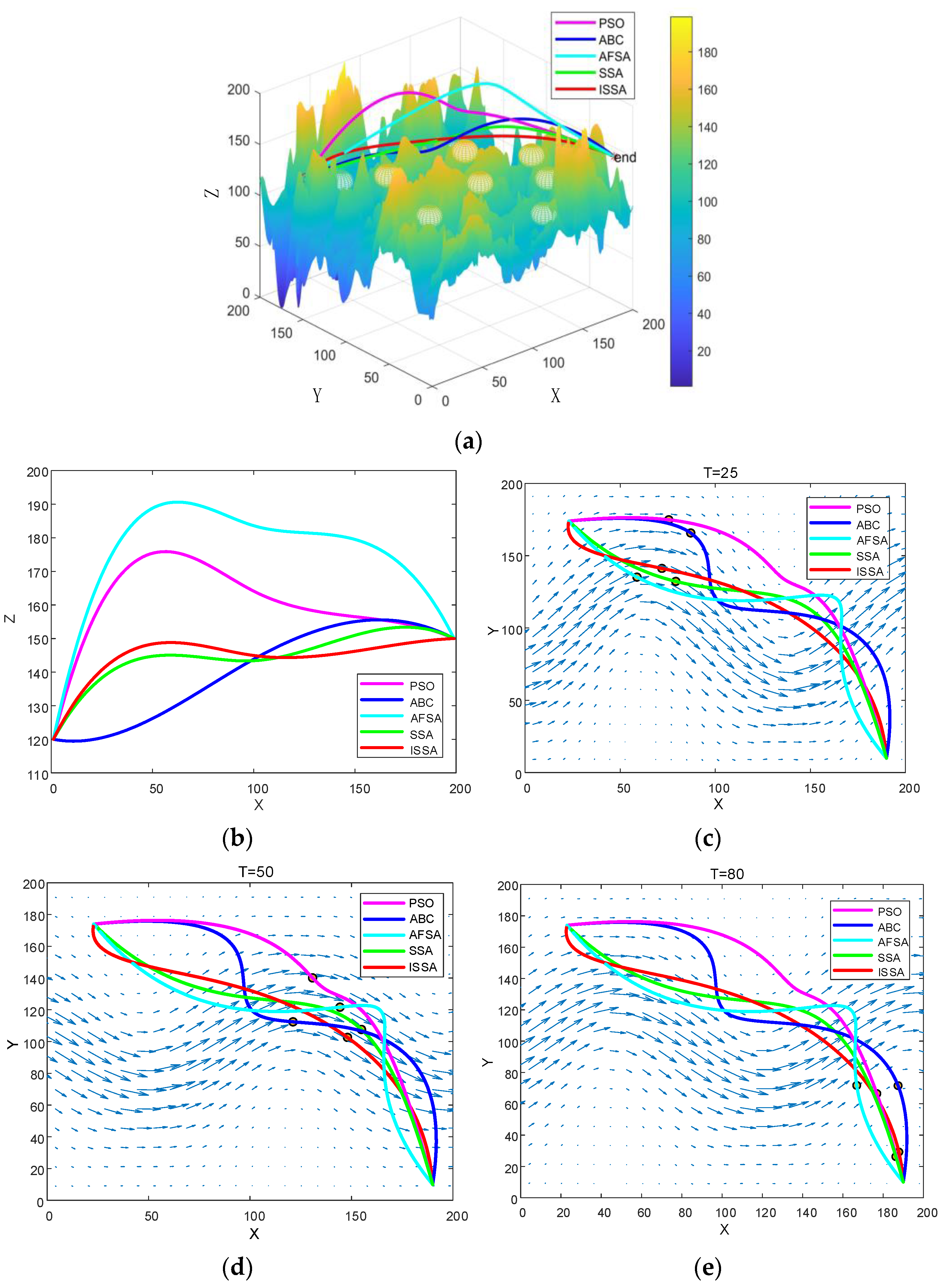
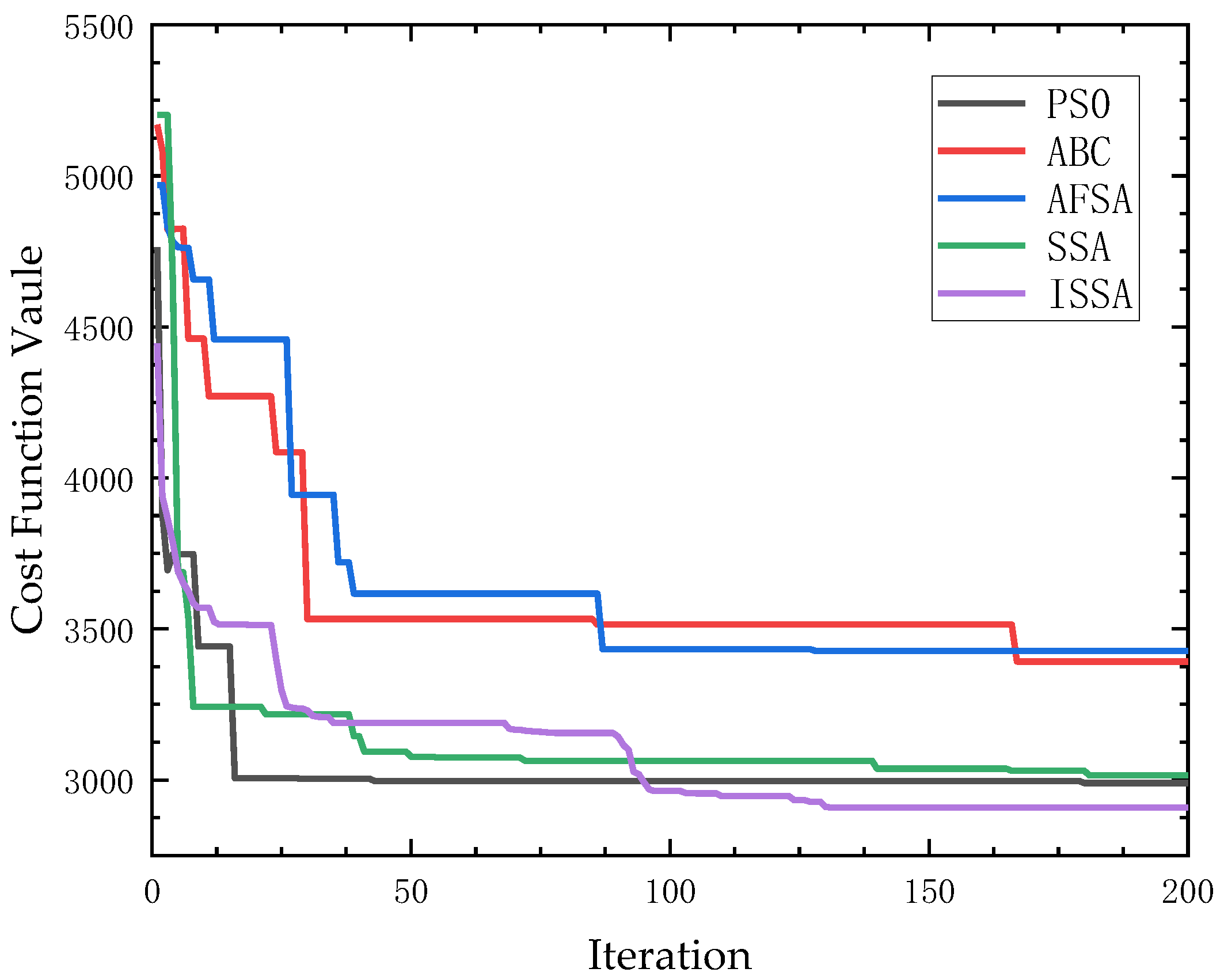
5.2. Comparison of Simulation Results in Distant Sea Scenarios

Distant sea areas are often faced with unfamiliar and complex terrains. Affected by ocean wind field, seawater temperature, salinity and density, ocean currents change greatly, and there are many non-topographic obstacles in such areas, such as large creatures and shipwrecks. Spherical obstacles are used to simulate these threats. This section takes the Pacific Ocean as an example to conduct a simulation study on the path planning of AUV in the distant sea scenario.

Figure 6 shows the path trajectory of the improved SSA and the other four algorithms in the distant sea scenario. Wherein, a and b are the route comparison map and side view in three-dimensional space, respectively, and c, d and e are potential field maps of current at T = 25, T = 50 and T = 80, respectively. The marked points in the figure are the navigation points corresponding to these times.

Table 6. Comparison of the results of each algorithm in the distant sea scene.

Algorithm	Best Value	Worst Value	Average Value	Standard Deviation
PSO	2818.51	3441.57	2975.58	135.79
ABC	3054.11	3793.68	3345.41	169.49
AFSA	3240.39	3781.73	3472.54	157.29
SSA	2762.27	3323.29	3015.51	132.24
ISSA	2777.45	3269.97	2908.54	122.14

shows the comparison of algorithms for AUV navigation results in the distant sea scenario.

Table 7. Comparison of error percentage of each algorithm in the distant scene. (Improved SSA as benchmark.)

Algorithm	Best Value Error Percentage	Worst Value Error Percentage	Average Value Error Percentage
PSO	1.48%	5.25%	2.30%
ABC	9.96%	16.02%	15.02%
AFSA	16.67%	15.65%	19.39%
SSA	−0.55%	1.63%	3.68%

is the comparison of cost error percentage, with the improved SSA as the benchmark. Figure 7 shows the cost curve of algorithms for AUV in the distant sea scenario.

It can be seen from the above figure that in the distant sea area, the improved SSA can not only plan a collision-free path but also the average cost is better than that of the other four algorithms. From the side view of the route comparison in Figure 6b, it can be seen that the improved SSA plans out a smoother height change than the other four algorithms, so the corresponding height change constraint is smaller. At first, it can be seen from Figure 6c that at the beginning of the planning, the path planned by the improved SSA and SSA can sail along the current direction and reduce the navigation cost. The AFSA algorithm goes against the current in the longitudinal direction, while the PSO and ABC algorithms are less affected by the current. Secondly, as time increases to time T = 50, it can be seen in Figure 6d that the improved SSA, SSA and ABC algorithms can make good use of the ocean current energy to sail and reduce the navigation cost. Finally, at the later stage of navigation, as shown in Figure 6e, the current at time T = 80 has little influence on the navigation trajectory and the navigation cost. Considering comprehensive AUV navigation at different moments, from the energy consumption constraint Equation (7), it can be seen that the improved SSA can use the ocean current navigation in the main navigation stages, and the navigation distance is shorter than that of other algorithms, so the energy consumption constraint is also smaller.

Table 7 is the comparison of cost error percentage, with the improved SSA as the benchmark. It can be seen that there is a gap between the AFSA algorithm and ABC algorithm compared with the improved SSA. There is a small gap between the improved SSA, SSA and PSO algorithm. This is because the three algorithms approached the extreme value in the optimization process, while the improved SSA is still better than the SSA and PSO algorithm in searching for the average value in the extreme value range. It can be seen from the above figure and table that in the distant sea area, the improved SSA has a smaller navigation altitude change cost and can make better use of ocean current energy to reduce the energy consumption cost. The global path cost is smaller than that of other algorithms.

6. Conclusions

Aiming at the navigation problem of AUV in the time-varying ocean current environment, this paper proposes a three-dimensional path planning method based on the improved sparrow search algorithm. According to the GEBCO database, the prior map information is obtained, and the continuous space submarine terrain information is approximately obtained by using the reciprocal difference method of adjacent point distance. The cost function is determined by combining the threat model, navigation height change model, underwater vehicle physical constraint model and energy consumption model under the time-varying ocean current environment, which need to be focused on in AUV path planning [32]. The experimental results show that the average cost of the improved SSA is lower than that of other algorithms in different cases. The improved SSA algorithm is used as a benchmark to determine the cost error percentage. The average cost error percentages of PSO, ABC, AFSA and SSA in the offshore sea scenario are 28.68%, 39.99%, 51.18% and 2.85%, respectively. The average cost error percentages of PSO, ABC, AFSA and SSA in the distant sea scenario are 2.30%, 15.02%, 19.39% and 3.68%, respectively. In this paper, we use a multi-strategy approach to improve the sparrow algorithm, which also makes the improved SSA algorithm perform better than other algorithms in the experiment. Therefore, applying the improved SSA to the three-dimensional path planning of AUV can effectively reduce the cost of AUV path navigation, avoid underwater obstacles and threats and use the velocity component of current to select the optimal path.

References

1. Cheng, C.; Sha, Q.; He, B.; Li, G. Path planning and obstacle avoidance for AUV: A review. Ocean Eng. 2021, 235, 109355. [Google Scholar] [CrossRef]
2. Teng, M.; Ye, L.; Yuxin, Z.; Yanqing, J.; Zheng, C.; Qiang, Z.; Shuo, X. An AUV localization and path planning algorithm for terrain-aided navigation. ISA Trans. 2020, 103, 215–227. [Google Scholar] [CrossRef] [PubMed]
3. Kim, J.; Kim, S.; Choo, Y. Stealth path planning for a high speed torpedo-shaped autonomous underwater vehicle to approach a target ship. Cyber-Phys. Syst. 2018, 4, 1–16. [Google Scholar] [CrossRef]
4. Kumar, S.V.; Jayaparvathy, R.; Priyanka, B. Efficient path planning of AUVs for container ship oil spill detection in coastal areas. Ocean Eng. 2020, 217, 107932. [Google Scholar] [CrossRef]
5. Sahoo, A.; Dwivedy, S.K.; Robi, P. Advancements in the field of autonomous underwater vehicle. Ocean Eng. 2019, 181, 145–160. [Google Scholar] [CrossRef]
6. Mandloi, D.; Arya, R.; Verma, A.K. Unmanned aerial vehicle path planning based on A* algorithm and its variants in 3d environment. Int. J. Syst. Assur. Eng. Manag. 2021, 12, 990–1000. [Google Scholar] [CrossRef]
7. Sun, B.; Zhang, W.; Li, S.; Zhu, X. Energy optimised D* AUV path planning with obstacle avoidance and ocean current en-vironment. J. Navig. 2022, 75, 685–703. [Google Scholar] [CrossRef]
8. Zhu, D.; Yang, S.X. Path planning method for unmanned underwater vehicles eliminating effect of currents based on artificial potential field. J. Navig. 2021, 74, 955–967. [Google Scholar] [CrossRef]
9. Che, G.; Liu, L.; Yu, Z. An improved ant colony optimization algorithm based on particle swarm optimization algorithm for path planning of autonomous underwater vehicle. J. Ambient Intell. Humaniz. Comput. 2020, 11, 3349–3354. [Google Scholar] [CrossRef]
10. Ma, Y.N.; Gong, Y.J.; Xiao, C.F.; Gao, Y.; Zhang, J. Path planning for autonomous underwater vehicles: An ant colony al-gorithm incorporating alarm pheromone. IEEE Trans. Veh. Technol. 2018, 68, 141–154. [Google Scholar] [CrossRef]
11. Cao, Y.; Wei, W.; Bai, Y.; Qiao, H. Multi-base multi-UAV cooperative reconnaissance path planning with genetic algorithm. Clust. Comput. 2019, 22, 5175–5184. [Google Scholar] [CrossRef]
12. Yuan, J.; Wang, H.; Zhang, H.; Lin, C.; Yu, D.; Li, C. AUV Obstacle Avoidance Planning Based on Deep Reinforcement Learning. J. Mar. Sci. Eng. 2020, 9, 1166. [Google Scholar] [CrossRef]
13. Zhang, Y.; Wang, Y.; Li, S.; Wang, X. Global path planning for AUV based on charts and the improved particle swarm opti-mization algorithm. Robotics 2020, 42, 120–128. [Google Scholar]
14. Yin, S.; Mao, J.; Li, B. AUV 3D Path Planning Based on Improved Empire Competition Algorithm in Ocean Current Environment. In Proceedings of the 6th International Conference on Computing, Control and Industrial Engineering (CCIE 2021), Hangzhou, China, 15–16 January 2021; pp. 36–49. [Google Scholar]
15. Cao, X.; Sun, C.; Chen, M. Path planning for autonomous underwater vehicle in time—Varying current. IET Intell. Transp. Syst. 2019, 13, 1265–1271. [Google Scholar] [CrossRef]
16. MahmoudZadeh, S.; Powers, D.M.W.; Yazdani, A.M.; Sammut, K.; Atyabi, A. Efficient AUV Path Planning in Time-Variant Underwater Environment Using Differential Evolution Algorithm. J. Mar. Sci. Appl. 2018, 17, 585–591. [Google Scholar] [CrossRef]
17. Cheng, Y.; Mei, Y.; Yu, J.; Su, X.; Xu, N. Three-dimensional unmanned aerial vehicle path planning using modified wolf pack search algorithm. Neurocomputing 2017, 266, 445–457. [Google Scholar]
18. Zhang, R.; Li, S.; Ding, Y.; Qin, X.; Xia, Q. UAV Path Planning Algorithm Based on Improved Harris Hawks Optimization. Sensors 2022, 22, 5232. [Google Scholar] [CrossRef]
19. Yao, X.; Wang, F.; Wang, J.; Wang, X. Energy-optimal path planning for AUV with time-variable ocean currents. Control Decis. 2020, 35, 2424–2432. [Google Scholar]
20. Eichhorn, M. Optimal routing strategies for autonomous underwater vehicles in time-varying environment. Robot. Auton. Syst. 2015, 67, 33–43. [Google Scholar] [CrossRef]
21. Xue, J.; Shen, B. A novel swarm intelligence optimization approach: Sparrow search algorithm. Syst. Sci. Control Eng. 2020, 8, 22–34. [Google Scholar] [CrossRef]
22. Li, M.; Xu, G.; Fu, Y.; Zhang, T.; Du, L. Improved whale optimization algorithm based on variable spiral position update strategy and adaptive inertia weight. J. Intell. Fuzzy Syst. 2022, 42, 1501–1517. [Google Scholar] [CrossRef]
23. Mirjalili, S.; Lewis, A. The whale optimization algorithm. Adv. Eng. Softw. 2016, 95, 51–67. [Google Scholar] [CrossRef]
24. Yıldız, B.S.; Pholdee, N.; Bureerat, S.; Erdaş, M.U.; Yıldız, A.R.; Sait, S.M. Comparision of the political optimization algorithm, the Archimedes optimization algorithm and the Levy flight algorithm for design optimization in industry. Mater. Test. 2021, 63, 356–359. [Google Scholar] [CrossRef]
25. Nautiyal, B.; Prakash, R.; Vimal, V.; Liang, G.; Chen, H. Improved Salp Swarm Algorithm with mutation schemes for solving global optimization and engineering problems. Eng. Comput. 2021, 7, 1–23. [Google Scholar] [CrossRef]
26. Noreen, I. Collision Free Smooth Path for Mobile Robots in Cluttered Environment Using an Economical Clamped Cubic B-Spline. Symmetry 2020, 12, 1567. [Google Scholar] [CrossRef]
27. Hu, Z.; Wang, Z.; Yang, Y.; Yin, Y. Three-dimensional global path planning for UUV based on artificial fish swarm and ant colony algorithm. Acta Armamentarii 2022, 43, 1676–1684. [Google Scholar]
28. Zhan, B.; An, S.; He, Y.; Wang, L. Three-Dimensional Path Planning for AUVs Based on Standard Particle Swarm Optimization Algorithm. J. Mar. Sci. Eng. 2020, 10, 1253. [Google Scholar] [CrossRef]
29. Karaboga, D.; Basturk, B. On the performance of artificial bee colony (ABC) algorithm. Appl. Soft Comput. 2008, 8, 687–697. [Google Scholar] [CrossRef]
30. Pourpanah, F.; Wang, R.; Lim, C.P.; Wang, X.-Z.; Yazdani, D. A review of artificial fish swarm algorithms: Recent advances and applications. Artif. Intell. Rev. 2022, 6, 1–37. [Google Scholar] [CrossRef]
31. Patil, V.S.; Bano, F.; Kurahatti, R.; Patil, A.Y.; Raju, G.; Afzal, A.; Soudagar, M.E.M.; Kumar, R.; Saleel, C.A. A study of sound pressure level (SPL) inside the truck cabin for new acoustic materials: An experimental and FEA approach. Alex. Eng. J. 2021, 60, 5949–5976. [Google Scholar] [CrossRef]
32. Guo, Y.; Liu, H.; Fan, X.; Lyu, W. Research Progress of Path Planning Methods for Autonomous Underwater Vehicle. Math. Probl. Eng. 2021, 2021, 8847863. [Google Scholar] [CrossRef]
Figure 1. Schematic diagram of B-spline curve optimization.
Jmse 10 01695 g001
Figure 2. Improved SSA algorithm AUV path planning flowchart.
Jmse 10 01695 g002
Figure 3. Three-dimensional terrain creation. (a) GEBCO plug-in display diagram; (b) 3D static environment map.
Jmse 10 01695 g003
Figure 4. Path trajectory in the offshore sea scene. (a) Route comparison map in 3D space; (b) route comparison side view; (c) sailing position at the moment T = 25; (d) sailing position at the moment T = 50; (e) sailing position at the moment T = 80.
Jmse 10 01695 g004
Figure 5. Variation diagram of optimal route cost in offshore defensive sea area.
Jmse 10 01695 g005
Figure 6. Path trajectory in the distant sea scene. (a) Route comparison map in 3D space; (b) route comparison side view; (c) sailing position at the moment T = 25; (d) sailing position at the moment T = 50; (e) sailing position at the moment T = 80.
Jmse 10 01695 g006
Figure 7. Variation of optimal route cost in distant sea scenario.
Jmse 10 01695 g007