1. Introduction
Fishing vessels are the most common ship type by number in the world, with 25,607. This represents 21.3% of the total world fleet, most of them being small- and medium-sized ships [
1]. In the case of Spain, its fishing fleet is one of the most important in relation to the number of vessels belonging to European Union countries, corresponding to 22% or 335,000 GT [
2]. In 2020, Spanish authorities had 8937 registered fishing vessels, the small- and medium-size fishing vessels being the most common [
3]. Furthermore, the daily work on board this type of vessel is considered to be some of the most dangerous, with the mortality per year very high in comparison with other sectors [
4,
5,
6]. According to the last report available from EMSA (European Maritime Safety Agency) about marine casualties and incidents [
7], from 2014–2020 a general decrease is visible in the average occurrence indicators of all type of ships, except for fishing vessels. A loss of stability, with the result of capsizing or large heeling, characterizes the type of accidents in which more deaths are registered than any other, in spite of many vessels being compliant with IMO (International Maritime Organization) stability regulations. However, the lack of stability is not only an issue related to fishing vessels, but also to merchant vessels and passenger ships in spite of the efforts of the IMO to improve stability requirements [
8].
The IMO current stability criteria might not consider the dynamic, heterogeneous and inconstant waves conditions that ships can encounter during the sea passage or during fishing tasks. As a consequence, since the start of the IMO and due to serious incidents occurring, specific research has attempted to understand and reduce the number of incidents related with stability. However, there are still produced accidents related to large amplitude motions, resulting in many cases in capsizing and the loss of lives. Among these undesired accidents, those which have most attracted the attention of researchers and institutions such as the IMO are the causes that lead to ships capsizing. For this reason, some research was carried out to improve the safety of, specifically, the fishing fleet. Mantari et al. (2011) [
9] studied the intact stability of ships, taking into account the actions of fishing gear loads and beam waves, and the wind influence, via a comparison of inclining and righting arms lever points of view for different operational conditions, including the influence of hull parameters and even the selection of fishing vessel machinery. Tello et al. (2011) [
4], through new operability criteria, proposed limiting values based on seakeeping calculations of several Portuguese fishing vessels in some sea states conditions, establishing certain hull shapes which optimize and fulfil the proposed criteria from an early ship’s design point of view. Mata-Santullano et al. (2014) [
5] studied the intact stability and operability characteristics of some Galician fishing vessels which were lost, and considered the stability curves in certain loading conditions, defined from KG and GZ values which allow us to fulfill the IMO intact stability criteria, but only in two sea state conditions. These results were confronted with decommissioned vessels, which ended their service life in a regular way and which were operated in similar conditions that sank ones. Míguez, et al. (2018) [
10] carried out an investigation to ascertain and obtain simplified models for roll response for medium-sized stern trawlers in regular beam and longitudinal waves and in static conditions. Alvite et al. (2020) [
2] proposed a new criterion for small Galician vessels (length less than 24 m) based on metacentric height (GM), dynamic stability and the value of the critical wave height according to specific Galician fishing grounds conditions. Santiago-Caaamaño et al. (2018) [
11] consider that most accidents in fishing fleets are caused by, among others, an incorrect operation of the ship and sailing in very bad weather conditions, which can lead to stability problems and, in consequence, sudden capsizing. For that reason, they proposed a guidance system which was as simple as possible based on naval architecture software and the Fast Fourier Transform which, without interaction from the crew, can predict automatically and in real time the ship’s initial stability based on natural roll frequency, transverse mass moment of inertia and displacement, although the proposed methodology was only tested on head waves. In the same sense, Santiago-Caamaño et al. (2019) [
12] proposed another system to monitor in real time the stability-integrating advanced signal processing, which was tested in beam seas but without considering the dynamic influence, especially the rough weather conditions. Although, obviously they are very interesting proposals, the question remains is if the small fishing vessel’s master would know how to interpret the presented values of GM, and most important, how they should proceed to decrease the risk level immediately with navigational parameters. Furthermore, some of the previously discussed research referred only to specific sea state conditions and static conditions, without considering the navigational parameters, which can be modified in real time by the duty officers.
Concerning merchant fleets, which also suffer stability and cargo shifting with the consequent claims, following Woo et al. (2021) [
13] the evaluation of ship’s stability only considering GM is not sufficient, because ships have to fulfill eight intact stability parameters. With that objective, a methodology was proposed with empirical formulas to calculate all these parameters once it has first calculated GM, in such a way that the duty officer can evaluate if a vessel is complying IMO requirements. Although a ship may fulfill the IMO requirement in static conditions, it will likely not do so in dynamic situations sailing in waves. For this reason, it is important to keep in mind that most of the operational life of ships takes place in the presence of waves, and occasionally quite severe conditions are faced. However, in some cases, fatal accidents have also occurred without facing extreme conditions, specified in the fishing fleet; in addition to the claims by damages, the shifting of cargo on board merchant ships can also produce the capsizing. This was demonstrated in the interesting research of Spandonidis et al. (2016) [
14], where systematic numerical research of granular material and vessel motion in regular and pure beam seas of different amplitudes was described.
Of the six degrees of freedom of a ship, the rolling motion is the most important, followed by the large amplitude motion and finally other dynamic effects which can produce the sudden loss of a ship [
10]. For this reason, the aim of this paper is to analyze the ship’s behavior in rolling motion, considering the navigational parameters involved in possible causes of capsizing, which are not treated by the current 2008 IS Code (IMO). The sudden loss of vessels is determined by the large roll angle at which downflooding occurs or when a synchronism situation is reached. Then, in order to reduce accidents improving the ship’s behavior, it is necessary that operators have the previous knowledge and tools about how they should proceed when the rolling motion starts reaching unacceptable levels for safety. Amongst the ship navigational parameters that a duty officer can alter immediately are the ship’s heading and speed. To do so, an officer needs to know how much time they have to alter these parameters, i.e., the specified time (t) elapsed from the rolling motion start at a certain loading condition until reaching a capsizing or downflooding situations. Therefore, in addition to the safe time frame available, the present work discusses also the headings and speed the ship’s operators need to adopt in order to conduct the navigation safely. These results are not only valid for fishing fleets, but also for others such as general cargo vessels, container vessels or RORO vessels. In these vessels, the avoidance of large roll angles is essential in order to minimize the possibility of cargo shifting, and to reduce the claims at the destination port and even diminish the loss of stability due to the lack of sufficient stability [
13].
It is important to note that the sudden losses of ships are concentrated in small fishing vessels [
15], specifically in some cases where the crew training in stability matters can be considered subpar. Therefore, in these ships the stability matters are arranged by the masters according to their own experience, i.e., without conducting a deep theoretical study of stability parameters [
11,
16]. This aspect was also mentioned in the last available report of the EMSA about analysis on marine casualties and incidents involving fishing vessels [
17] where it is considered that not correctly assessing of the vessel’s limitations (bad weather conditions) had contributed to listing/capsizing accidents. For this reason, it is essential to provide these crews with the tools and knowledge, and to make it as easy as possible to act accordingly, altering speed and heading in order to deal with unforeseen wave conditions. However, capsizing is a dynamic phenomenon, from a stability and environmental conditions point of view. Thus, if the operator’s stability training is subpar, understanding these motions while a ship is sailing in bad weather conditions can be a little difficult for them. This is due to lack of knowledge of dynamic stability and the large number of parameters involved. With the objective of minimizing the probability of accident, specifically large-amplitude roll angles and capsizing, in this paper a new methodological proposal is proposed to be used by ship operators in order to improve the seakeeping, considering parameters very easy to use and obtain. The first parameter for controlling the stability is the ship’s loading conditions, expressed as natural roll period (Td), which can be easily measured by any sailor in calm conditions. The second parameter is the waves’ period (Tw), measured on board and taken as reference to determined points along the ship’s length and, finally, the encounter period (Te), which can be calculated using a very simple equation.
Operability is a very important factor for the ship’s master in order to establish vessel safety. As limited literature analyses maneuverability in waves, this paper intents to deal the maneuverability and seakeeping jointly, despite the fact that in the literature they were typically treated separately. Furthermore, the present research can be considered as a continuation of previous research carried out by authors [
18] about the study of ship motion around the longitudinal axis, i.e., the rolling motion. In that case, the ship’s rolling motion sailing between pure beam waves was studied, both without resistance and in static conditions. The aim of the present paper is to carry out research about the ship’s behavior from a point of view closer to reality, studying the ship’s performance sailing in any type of waves, with resistance and the ship being hit from any influence angle. Thus, the optimal heading and speed to be set by the ship’s operator are being studied implicitly in order to keep the sea passage as safe and comfortable as possible. Furthermore, the specified time (t) elapsed from the rolling motion start until a capsizing or downflooding situations occurs is being studied in order to give to masters an idea about the available time to modify or alter certain parameters. For this mission, different mathematical models were applied to rolling motion, which is independently studied in the following sections.
2. Materials and Methods
As the ship’s behavior leading to capsizing in irregular waves is similar to that in regular waves [
19], in the first subsection in which it is presented the mathematical models of regular waves corresponded to any sea state conditions registered. Secondly, the mathematical model which represents the ship’s rolling motion sailing in pure beam waves and with resistance was studied. Finally, considering the two previous sections together, the mathematical model that allows for determining the ship’s behavior of sailing, while receiving the waves from any constant direction and considering the ship’s navigational parameters which can be modified by the master, is studied i.e., the speed and the heading.
2.1. Waves
As was already established in previous research, it is difficult to accurately predict the ship motion in irregular seas [
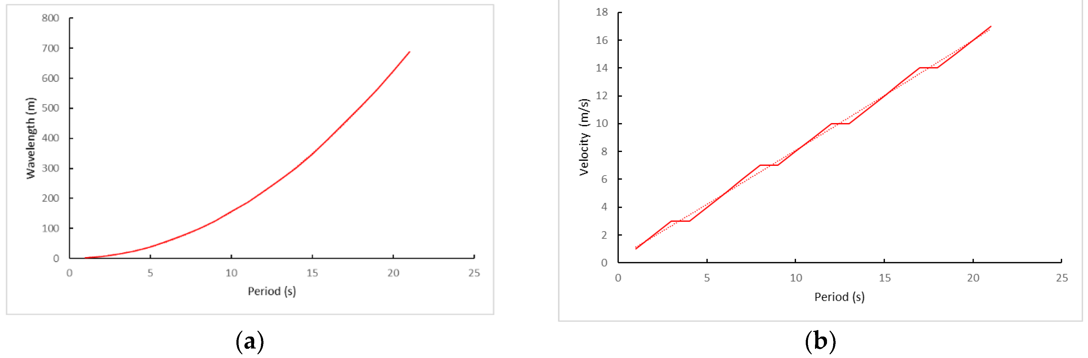
18]. Thus, as usual, the waves with a trochoidal profile, which correspond to tender regular sea (after the wind ceases), are studied here from a mathematical point of view. In the field of waves’ study, three parameters have always been considered: wavelength (Lw), translation velocity (Vw) and period (Tw). With that objective, empirical observations of any sea state condition have allowed the building a scale of 21 types of waves relating to these three parameters. Considering the values of the period (Tw) and the registered empirical observations, the following several polynomial regression equations were obtained (wavelength in m; velocity in knots and velocity in m·s
−1), as a function of wave period.
In
Figure 1 the high precision for the determination factor of Equations (1)–(3) can be observed.
However, one of the easiest and most practical parameters for sailors to use is the wave amplitude (Aw), i.e., half of the height (Hw), so it was necessary to relate it with the three previous parameters (wavelength, period and velocity). However, as the wave height (Hw) is affected by, among others, the fetch and duration of the wind swell generator, there are no formulas which allow the linking together of all these parameters. Nevertheless, it is possible to link the maximum wave slope (θ
MW) with the wavelength (Lw) and the height (Hw), as is shown in the following equation.
The empirical observation of waves around the world has allowed for registering the wave characteristics [
20], concluding that θ
MW, regardless of smooth or very rough sea, is almost constant and equal to 0.1047 (6°). Therefore, with the help of Equation (4), and wavelength calculated according to Equation (1), Hw and Aw can be obtained.
Table 1 includes all data calculated according to Equations (1)–(4) for the full spectrum of regular waves considered in the present research.
2.2. Rolling Motion in Static Conditions and under the Influence of Beam Waves with Resistance
In reality, the free rolling motion produced by an external and punctual force is affected by the resistance of water and air, which cause the roll angle amplitude to be damped until the ship is at rest again. In the case of air resistance, its value is very low, therefore, its practically null effect on roll damping means that air resistance can be disregarded. The same does not happen with water resistance, so the inertia moment, the moment of water resistance and the ship’s righting torque are involved in the equation of the ship’s rolling motion sailing in beam waves with resistance. In the ship’s righting torque (Ma) the angle of wave’s slope, θ
w, is introduced so in the initial stability, i.e., for low rolling angles, it can be established:
where D is the ship’s displacement; GM is the initial transverse metacentric height; and (θ − θ
W) is the angle of relative rolling between the normal to the wave’s slope and the diametrical plane. In consequence, the equation of the ship’s rolling motion sailing between transversal waves and with resistance is expressed as follows:
where Ig is the inertia moment of the ship’s mass about a longitudinal axis through its center of gravity and A
R is a damping coefficient.
Considering that in regular seas it is common that the angle of wave’ slope is low compared to the absolute rolling angle between the perpendicular to the surface of the water in calm conditions and the ship’s center line, Equation (6) can be simplified as follows:
Now, several transformations on Equation (8) are performed with the aim of obtaining the relationship between rolling periods. So, in the first stage Equation (8) is divided by the inertia moment Ig:
Knowing that the inertia moment is:
where g is the gravity acceleration and k is the turning radius of the ship’s mass with respect to the longitudinal axis passing through its center of gravity.
Operating for convenience:
Replacing Equations (10) and (11) in Equation (9):
Knowing that natural roll frequency is;
Equation (14) is now introduced in Equation (13):
In Equation (16), the first three terms match with the general equation of the rolling motion sailing in calm water conditions with resistance, the fourth term (
) being the disturbing (induced) force of the waves. When studying the rolling motion of a ship sailing in waves without resistance, the same disturbing force of the wave’s slope is obtained, being the resulting term;
Replacing Equation (17) in Equation (16):
If it is taken as a particular solution of Equation (18),
And Equation (19) is derived twice:
Replacing the particular solution and its derivatives in Equation (18):
Taking out common factor
and
of Equation (22):
Equation (23) must satisfy any value of t, and for that mission it is necessary that
Clearing F
K in Equation (25):
In order to find E
K,
is cleared in Equation (24) and the value of F
K found is introduced;
Taking out common factor E
KThis Equation (32), according to Equation (26), can be also expressed as follows:
Developing the trigonometric relationship:
The first term of Equation (37) is equal to the first parenthesis of the first term of Equation (31), therefore:
Equation (19) is divided by E
K, which is the particular solution of the differential equation of the ship’s rolling motion between waves, in which the resistance of water Equation (18) is considered, and considering Equation (32):
Then, the absolute rolling angle is equal to:
If in Equation (44) E
K is replaced by its value of Equation (39):
Equation (48) is similar to the equation of rolling motion induced by transversal waves, but without the resistance studied in the previous research of authors [
18], although it is now included by the β angle, which depends on damping factor λ. Thus, the rolling angle of Equation (48) is the angle of rolling motion induced by waves’ disturbances.
According to Equation (48) and with the equation of rolling motion in calm water conditions with resistance [
21], the equation of a ship’s rolling motion sailing in waves and with resistance can be expressed as follows:
The first term represents the damped rolling, where λ is the factor damping and θM is the initial maximum angle of roll.
If the damping factor is equaled by a factor sub-1 by time unit:
In addition, the ships’ and the waves’ frequencies are replaced by their corresponding periods (Td and Tw), Equation (49) is:
Moreover, considering that:
Numerator and denominator of the second term of Equation (52) is divided by ω
2:
Equation (53) can be expressed, taking into account the corresponding periods (Td and Tw):
2.3. Rolling Motion in Underway Conditions and Under the Influence of Waves of Any Constant Direction
In this section, the ship rolling motion for when waves are hitting it from any constant value of α angle is analyzed, formed between the ship’s center line (heading), which can be modified by the duty officer, and the waves’ direction.
According to basic plane trigonometry, the encounter velocity (Ve) can be expressed as follows:
where Vw is the waves’ velocity and Vs is the ship’s velocity. Furthermore, considering that the relationship between the waves’ length (Lw), the waves’ period (Tw) and the waves’ velocity (Vw) is:
It can be expressed in the following relationship:
Replacing in Equation (58) the encounter velocity (Ve) given in Equation (56):
The term is positive when α is in the first or fourth quadrant (when the swell comes from port and starboard bow), and negative when is in the second and third quadrant (when the swell comes from port and starboard quarter), considering the line forward-aft as a positive axis. According to Equation (59), when the ship receives the waves from the bow, the encounter period (Te) is lower than the wave period (Tw); when it receives them from the quarter, the encounter period is higher than the wave period.
The wave’s slope depends on its length (Lw) and height (Hw). Decomposing the incoming wave in a longitudinal and a transversal wave, the length of the last one (L
BEAM) is:
As a consequence, the transversal component of the wave’s slope is affected by sin α and by the maximum wave’s slope (θ
MW ROLLING), which is of interest in the study of induced rolling motion:
Therefore, Equation (51) of rolling motion sailing in waves with resistance can be generalized by introducing the encounter period (Te) and the maximum wave’s slope of the transversal component, which can be expressed as follows:
Considering that, according to Equation (55);
The obtained Equation (62) represents the real rolling motion of a ship in waves, where the two navigational parameters are included. This can be adjusted by operators at any time, as can the heading and ship’s speed. The heading is included in the second term as sin α, and the ship’s speed is indirectly included in the Te variable, while at the same time it also has influence the heading (α). Furthermore, that the rolling angle is a function and changes with the time (t) has been shown, and so in the Results section a deep analysis applied to the case studies is carried out.
3. Results
This section provides a study of a ship’s behavior, expressed as a function of the rolling angle reached in the linear time domain. In the first subsection, the rolling motion in static conditions was analyzed under the influence of beam and regular waves with resistance. In a way, this approach is considered to be interesting due to it being the worst situation found when the ship was at zero speed. Following the same approach, afterwards the rolling motion was studied from a more realistic point of view, i.e., when the ship’s movement is underway at any ship’s speed and heading, and under the influence of all registered waves coming from any direction.
In order to validate the obtained results in the previous section checking that they are valid to any sea state condition, simulations were conducted with the 21 swell conditions, which were previously modelled in Equations (1)–(4).
For the objective proposed in this paper, the mathematical models, the appearance of figures and the general conclusions obtained from them are the most important aspects of this paper. For the case study used for validations, the usual parameters found in some of the fishing vessels of the Spanish fleet were selected. These have lost stability in the last 20 years, resulting in the loss of many lives. Although the exact loading condition in the moment when an accident happens is unknown, Bonilla de la Corte (1994) [
22] considers that usual Td for fishing vessels is between 8 s and 14 s. Furthermore, in Bonilla de la Corte (1994) [
22] we can find that Td can be estimated as follows:
where B is the beam and GM is the metacentric height.
Moreover, the classification society DNV (2016) [
23] considers that the relationship between GM and B is the following:
In addition, according to DNV (2016) [
23], knowing the beam (B) and the metacentric height (GM), the Td can also be calculated by the following equation:
Then, included in
Table 2 are the most relevant data of several capsized fishing vessels, and the calculated Td according to previous equations.
Obviously, Equations (64)–(66) only allow for an estimated idea of Td and GM. This is because the exact value of both parameters depends on the specific ship’s loading condition, expressed as natural roll period (Td). For that reason, from the proceedings literature it can be extracted Td values are substantially different from those calculated as per the mentioned equations. Miguez et al. (2016, 2017, 2018) [
24,
25,
26] consider that, in a trawler fishing vessel with a beam of 8.0 m, the Td assigned was between 11.1 s and 10.3 s, while the calculated Td according to equations would be 8.2 s. Oliva-Remola (2017) [
27] considers that in a trawler fishing vessel with a beam of 11.50 m, the assigned Td was 10.6 s, and the calculated Td was 9.9 s.
Considering the above, and with the objective proposed in this research of being as generic as possible, a natural roll period (Td) of 9.0 s can be considered representative enough of the type of fishing vessel fleet which has sustained problems in terms of the stability of sailing on waves. This value is in line with the Td values used in previous works [
12], where the models were evaluated with 7.8 s < Td < 12.2 s for a fishing trawler with a length of 34.5 m and a beam of 8.00 m.
Regarding the initial maximum angle of roll, θ
M, 10° was considered in our simulations, understanding that, in bad weather conditions, it can be a roll angle easily reached by medium-sized fishing vessels. In terms of the roll-damping factor, λ, following recommendations of the literature review [
28,
29], a median coefficient of 0.015 was selected. As the roll-damping factor depends on each rolling angle reached, and they are not constant, the results of proposed models can be considered as simplified and a first approach to be validated in scale model tests or in computer programs. There, the influence of different underwater shapes (bilge keels or not), block coefficients and appendices as different types of roll stabilizations systems (active fins) could be discussed.
3.1. Rolling Motion in Static Conditions under Beam—Regular Wave’s Influence with Resistance
In this subsection, the ship’s performance during rolling motion is calculated from a mathematical point of view, both for when the ship is in static conditions and receiving the waves from beam, although with resistance.
Analyzing the first term of Equation (49) and the variation with the time (t) of the damped rolling, it is concluded that when the ship is with zero speed and under pure beam seas influence, it would end up disappearing due to its decreasing geometric (
) quality. Theoretically, the ship would end up rolling according to the waves’ period (Tw) instead of its natural roll period (Td), i.e., according to the second term of the equation, which corresponds to the induced rolling (forced), reaching a synchronism condition. However, due to the lack of regularity in the waves and the tendency of a ship to roll according to its natural period, in the reality it is usual that synchronism is not reached. Considering this premise, the maximum rolling angle is produced with the following periodicity:
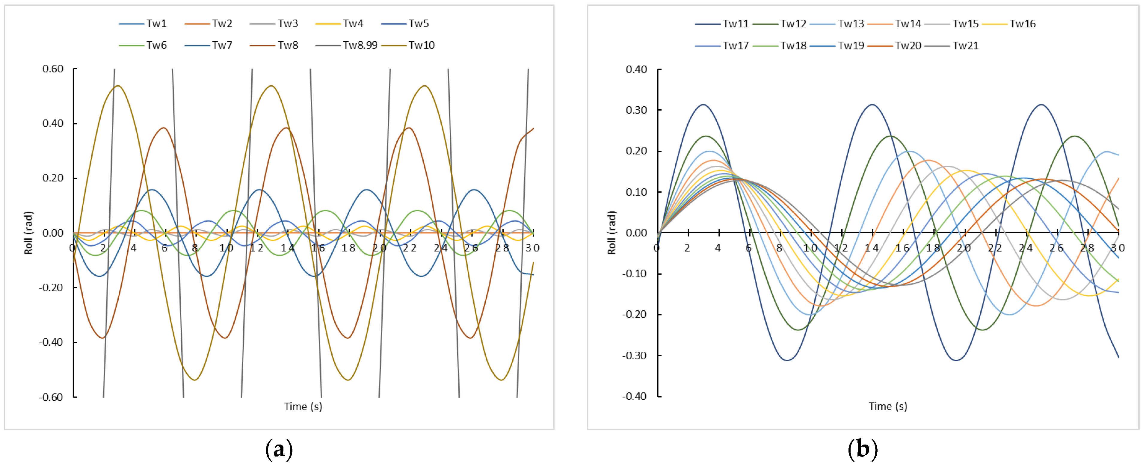
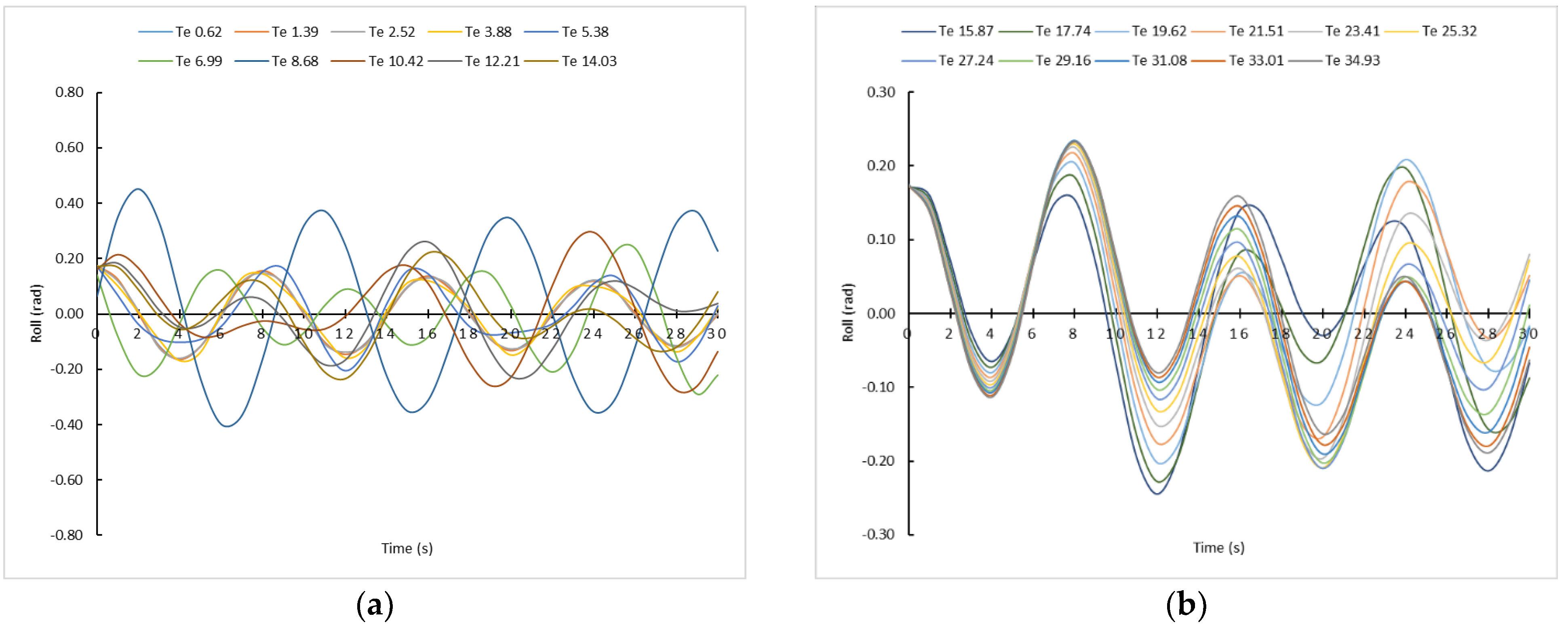
This interesting conclusion expressed in Equation (67) can be corroborated in
Figure 2, where it was represented by the rolling motion under the influence of the 21 types of waves (Tw). For clarifying purposes, the representation was divided into two graphs, i.e., from Tw = 1 s to Tw = 10 s (
Figure 2a), and from Tw = 11 s to Tw = 21 s (
Figure 2b). Furthermore, it is observed that, with Tw = 8.99 s, it theoretically produced the synchronism phenomenon (Td = Tw), with the appearance of asymptotic curves. However, another relevant result is that the amplitude of rolling for Tw = 8 s and Tw = 10 s is not the same, even though both are 1 s apart from the Tw = 9 s.
Moreover, although the relative maximum rolling angle is reached according to our results expressed in Equation (67), it is also noted that the maximum amplitude does not always have the same value, and it varies as time increases. The reason for this is that the amplitude of roll depends on cos β in such a way that, as β increases, the roll angles decrease, being consistent with the water resistance.
Another relevant observation is that the absolute maximum angle is not always reached in the first moments, as it can be deduced from, for example, Tw = 11 s and Tw = 12 s. That is to say, maybe that master would have enough time to act and then, improve the ship’s behavior, for example, modifying the Td, i.e., ballasting, deballasting or transferring the ballast vertically.
3.2. Rolling Motion in Underway Conditions and under the Influence of Waves of Any Constant Direction
In this subsection the ship’s behavior in rolling motions closest to the reality experienced by a ship during the sea passage is studied, i.e., for a given ship’s speed and heading. The last component, together with the waves’ influence direction, defines the angle α, i.e., the angle formed between the ship’s heading and the waves influencing direction.
Once analyzed in deep the Equation (62), it is observed that the first term is related with the damped factor rolling, and then that it will decrease geometrically (
) as time (t) goes on. In consequence, over time, the roll motion will be determined by the second term of Equation (62), i.e., following to encounter period (Te) and the angle α of influence of the waves. According to this reasoning, and considering the ship’s speed and heading as constant, the maximum roll angle is reached when:
In order to validate our conclusion mentioned in Equation (68), and according to Equation (62), it is necessary to establish the ship’s speed (Vs) and the α angle. The Vs can be considered between 0–12 knots, and the α angle between 000° and 180°, regardless of whether the waves are received from port or starboard side. This is because the only difference is the rolling side, not the amplitude or the moments (t) when a certain roll angle is reached. As it is not practical to represent here all the graphs for all these combinations, in this paper the simulations carried out are shown, with a selected speed of 8 knots and an α angle of 45°, i.e., for receiving the waves by the bow. In
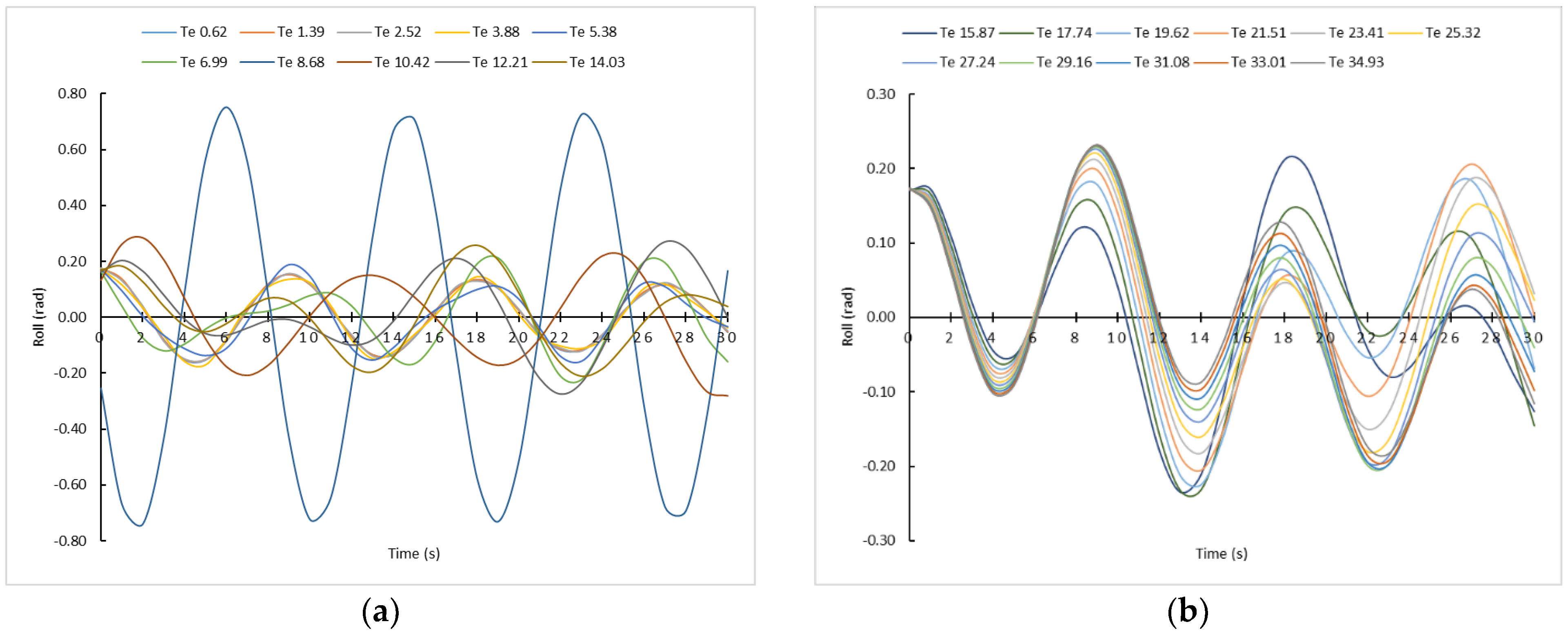
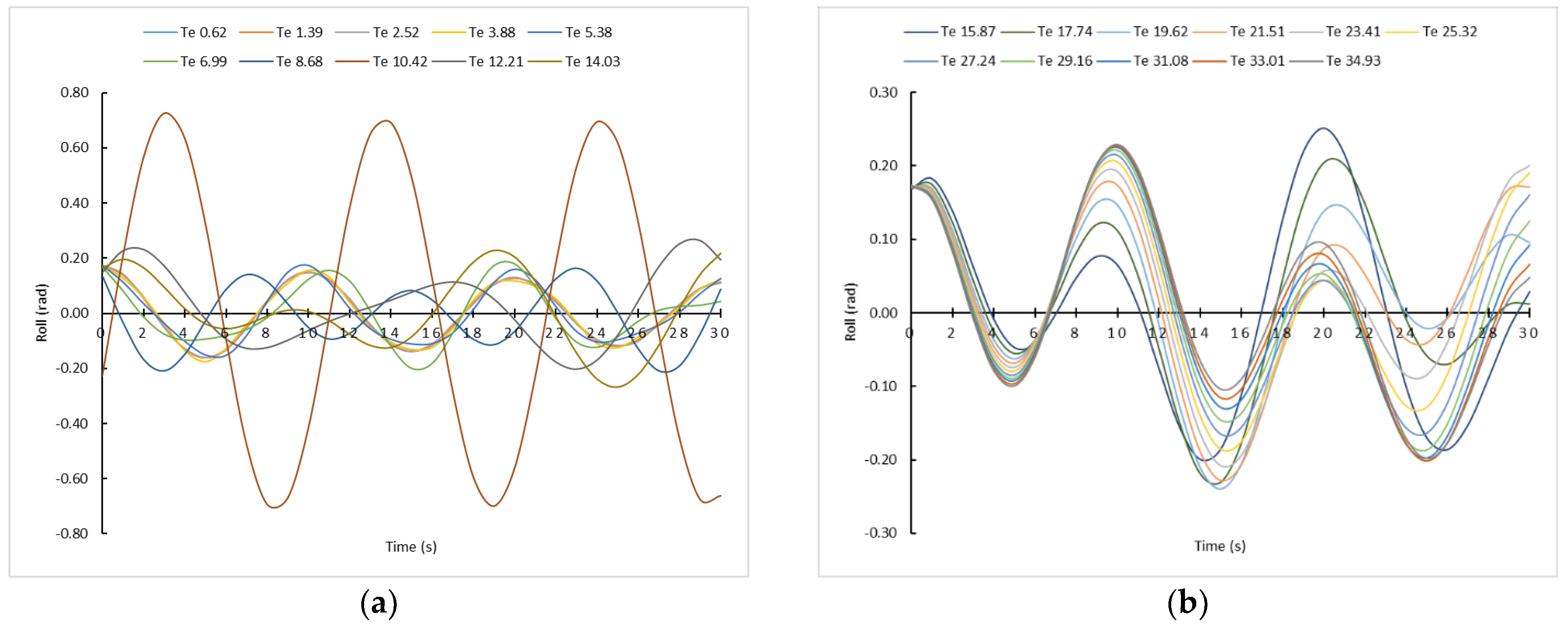
Figure 3, the influence of all sea state conditions (21 types) is depicted in a ship with the parameters commented above. In this case, unlike those established in the previous subsection, the influence of waves is represented through Te instead of Tw. As it is shown, in all sea state conditions our Results expressed in Equation (68) are satisfied.
As it can be observed from
Figure 3a, with a Te = 8.68 s, corresponding to Tw = 7 s, the ship would reach a roll angle of about 0.75 rad (43° approx.). However, no asymptotic curve corresponding to the synchronism phenomenon is observed, although theoretically it should be registered. For this reason, it is noted that, in real situations, Te must be analyzed in depth, far more so than Tw. This consideration is considered important because, although waves’ characteristics found at sea cannot be modified, the ship’s master can influence Te, altering the ship’s speed and/or the heading.
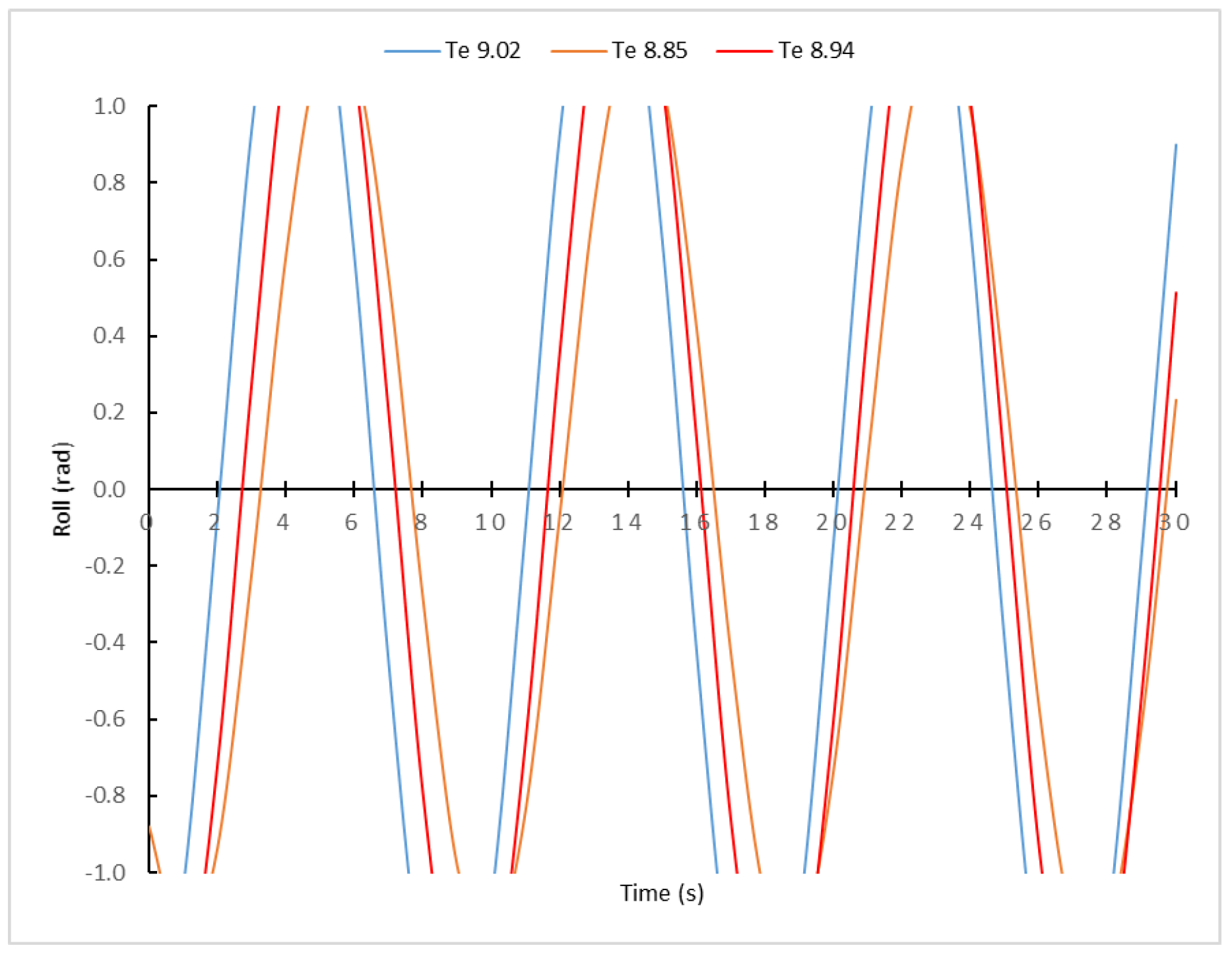
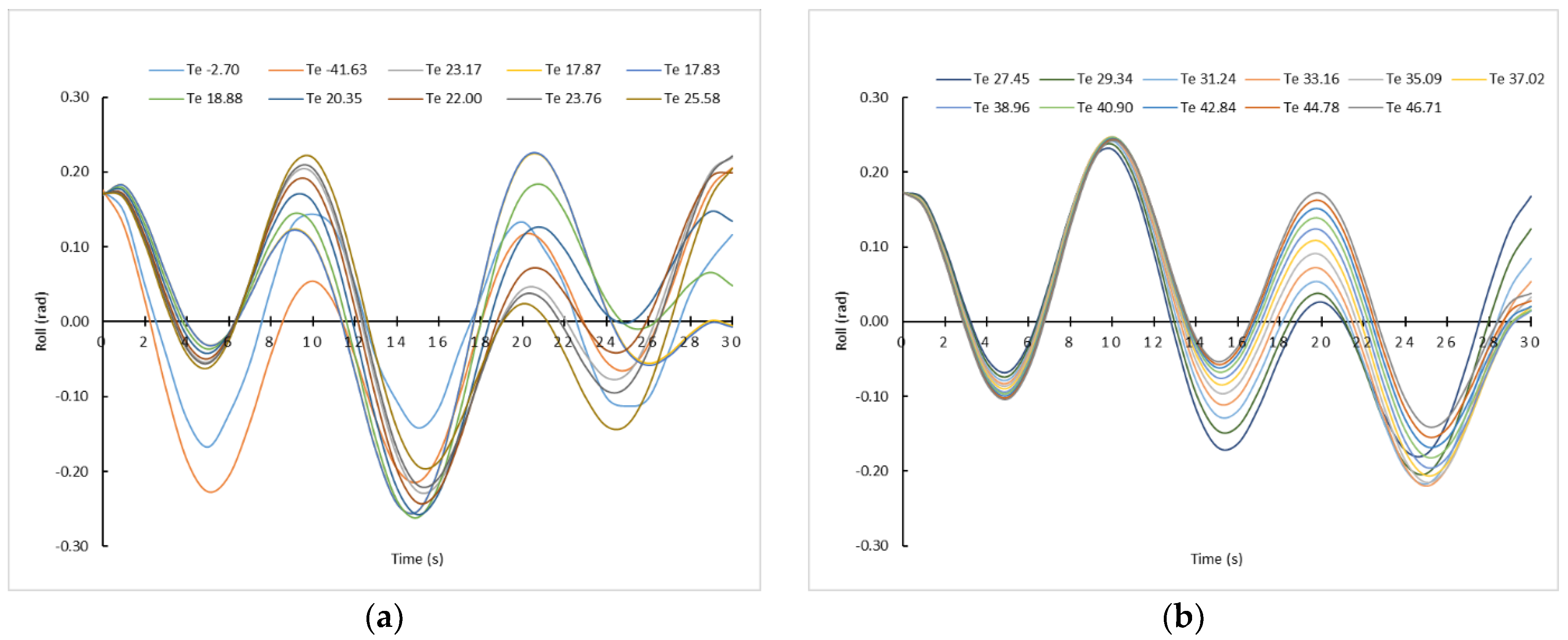
In order to check more in detail what the worst Te, and in consequence the Tw, are to face the rolling motion, in
Figure 4 the rolling motion was represented for Te = 8.85 s (Tw = 7.1 s); Te = 8.94 s (Tw = 7.15) and Te = 9.02 s (Tw = 7.2 s). For that, it was necessary to appeal to Equations (1)–(3) of waves, which were previously modelled. In
Figure 4, it can be observed how the curves tend to be asymptotic, being a dangerous situation for the ship’s safety, even though all the ship’s parameters were in keeping with the optimal range. Therefore, with the results presented here, it is demonstrated that it is necessary to carry out a more detailed analysis of each sea state condition in order to not compromise the ship’s stability. Then, if ships masters pay attention only to the categorization of the sea state according to the wave period (Tw) typical from the weather forecast, for example, they can think that the ship is sailing in a more or less safe situation, when this is not the case.
4. Discussion
In our simulations, 10° was considered to be the initial maximum angle of roll. If we consider that initially the ship is in the upright position it is relevant to note that, in simulations with the ship in a static position and between pure beam seas, as it can be observed in
Figure 5, for Tw = 8 and 10 s the amplitude of the maximum rolling angle is lower than when the initial maximum roll is 10°. In the rest of the wave conditions (Tw), the amplitude of the rolling angle is lower with the ship initially in an upright position. Therefore, depending on which position is taken as the origin of time (t), the obtained results can be surprising, because as it is shown, it would be better that initially the ship has a maximum roll angle of 10° that it would be upright position, something that goes against good seamanship.
In dynamic conditions, with respect to the parameters simulated in our research referred to real conditions, i.e., Vs = 8.0 knots, α = 45°, θMAX = 10° and Td = 9 s, if Td is altered from 9 s to 8 s and 10 s, i.e., the closest loading conditions which can be reached most easily during sea passage altering weights, relevant conclusions are obtained too.
As it can be observed in
Figure 6, with Td = 8 s, the amplitude of maximum roll angle is greatly reduced almost in half for Te = 8.68 s (Tw = 7 s), i.e., for the same sea conditions that with Td = 9 s. It is evident that if the ship’s operators are alert well in advance, the fact of reducing 1 s the Td, can suppose avoid very dangerous situations or even the ship’s capsizing. In the other Te conditions, the amplitude of angle rolling is almost the same.
However, if simulations are carried out with Td = 10 s, the most important variation is the Te (Tw) condition in which the maximum amplitude of roll is reached, in this case Te = 10.42 (Tw = 8 s). For other waves’ conditions, as it can be noted in
Figure 7, the amplitude of maximum roll angle hardly changes, except obviously the moment (t) when these relative maximum roll angles are reached, as was concluded previously in the Results section.
As is shown in
Figure 8, if the ship’s operator decides to change the ship’s heading so that an α angle of 120° is reached, the ship’s behavior and the maximum rolling angles are substantially improved. There are hardly any significant variations between the different sea state conditions.
Once again, it is clear the importance for ship’s operators not only to control the ship’s loading conditions to improve the ship’s behavior sailing in waves, but also to control the waves’ parameters and the navigation parameters as the ship’s speed and heading, which are included in Te variable. Furthermore, sailing in waves conditions, it is shown again that it is more important to verify Te than Tw, with the consequence that maybe Tw lower implies a worse ship’s behavior.
It is worth mentioning that, sailing in longitudinal waves (α =000° or 180°), theoretically no rolling motion is registered, so it is an option that the master should be in mind. However, in bad weather conditions receiving the waves exactly by the bow or astern are not recommended for safety of seakeeping conditions due to different factors as slamming, propeller’s emergence and others.
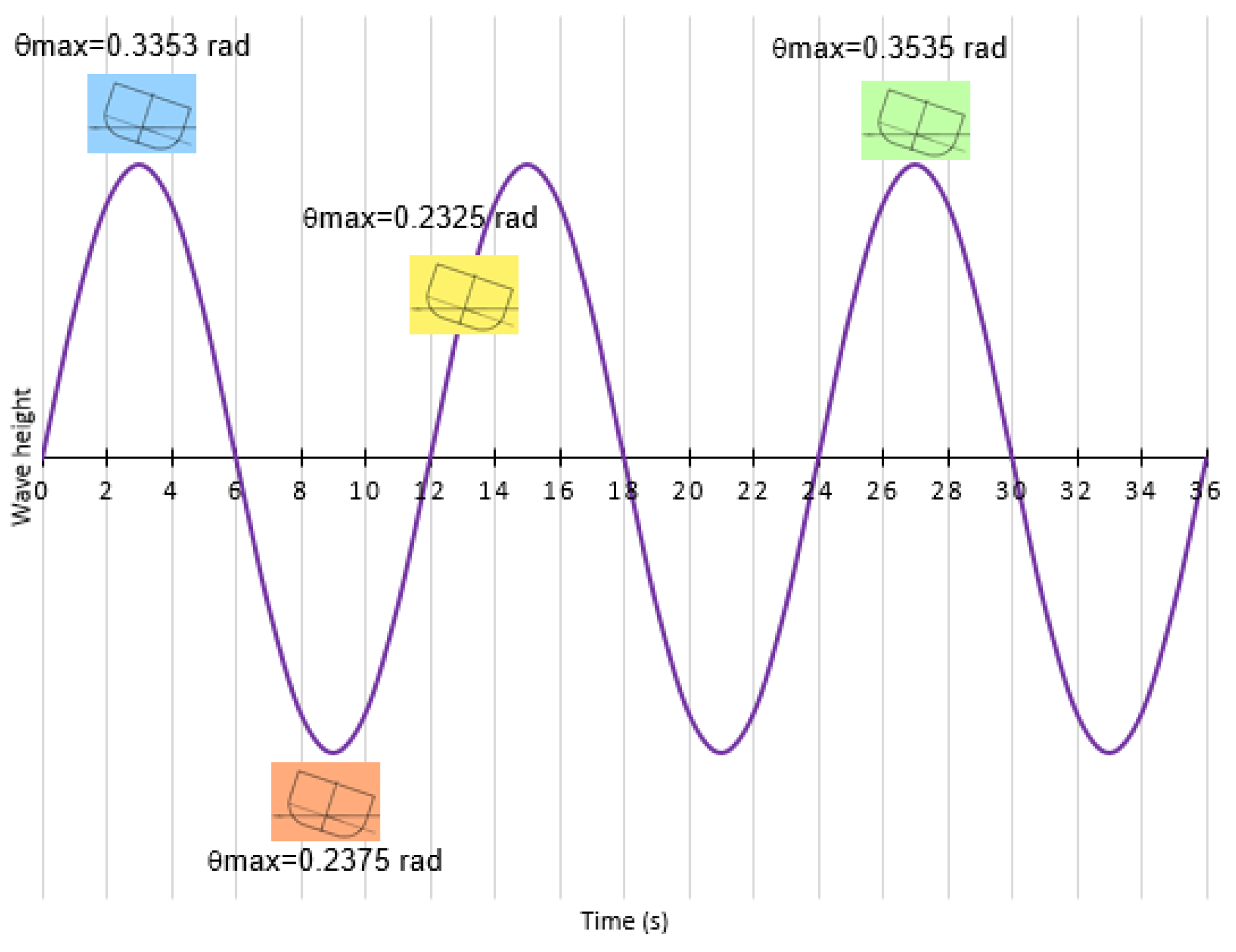
Finally, in
Figure 9 a schematic diagram of waves with period of 12 s (Tw), which corresponds with a height of 7.42 m and a ship with a loading condition of Td = 9 s. Over the wave profile, it is shown the maximum rolling angle and the moment (t), when they are reached, and in different situations as are the follows:
In static conditions, under a beam wave’s influence without resistance (blue colour).
In static conditions, under the abeam waves influence with resistance (green colour).
In dynamic conditions, sailing with a ship’s speed of 8 knots and an α angle of 45° (orange colour).
In dynamic conditions, sailing with a ship’s speed of 4 knots and an α angle of 120° (yellow colour).
In this
Figure 9, it is graphically shown that, in dynamic conditions, in some cases, the fact of altering substantially the combination between heading and ship’s speed there hardly causes differences in the maximum rolling angle reached, but the time to reach this rolling angle changes considerably. Furthermore, it is also relevant that the maximum rolling angle in static conditions and realistic conditions (with resistance), under the influence of pure beam seas, is reached at 27 s, i.e., quite some time after starting the rolling motion, unlike what happens in dynamic conditions and in theoretical conditions (pure beam seas without resistance).
5. Conclusions
In this research, the ship’s behavior was studied and modeled in rolling motion at zero-speed conditions with beam seas, as well as in underway conditions receiving the waves from any direction. Once the corresponding models had been obtained, it was concluded that as time goes on, in static conditions, the ship will roll according to waves’ period (Tw) instead of its natural roll period (Td), and that in dynamic conditions, the ship will roll according to the encounter period (Te) instead of Td or Tw. As in the Te value, the heading and ship’s speed and included, and it is essential that ship operators have under control the influence of Te in the ship’s behavior. What is more, these results permit vessel operators to know how they must proceed in order to change heading and/or ship’s speed to improve the ship’s behavior, from a scientific point of view and without leaving these changes at discretion of master experience. This is required because the watch officer can be a novice operator without the necessary experience to face adverse conditions. Furthermore, given that the particular sea state conditions are imposed during the sea passage, it of the utmost importance for ships’ operators to know the navigational parameters (heading and speed) or the loading conditions to be set, modified or avoided. Thus, using the obtained models several simulations were carried out in order to obtain relevant results. For a given loading condition (Td), the available time (t) before reaching the maximum rolling angle that ships’ operators have in order to act and thus change the ship’s behavior was obtained. This is a direct function, in static conditions, of waves’ period (Tw), expressed as and in dynamic conditions, of the encounter period (Te), shown as . Knowing the available time (t) before reaching the relative maximum angle is essential in order to alter the navigational parameters (heading and speed) or even the loading condition, ballasting, deballasting or transferring ballast. It must be taken into account that reaching high rolling angles compromises the safety of the ship, crewmembers and cargo, and can even produce capsizing or reaching a downflooding angle.
The action of change of heading and ship’s speed is a usual procedure followed by ship masters in order to improve the ship’s behavior when sailing in rough seas. However, these changes are left in many cases to the discretion of master experience or based on empirical facts experienced in real time on which the master adjusts according to ship’s performance, i.e., without considering an objective and scientific analysis. Through the case studies included in the Discussions section, it was demonstrated, from a scientific point of view, that through modifying the loading condition or altering the heading, the ship’s behavior improves and the maximum relative rolling angle reached is reduced very considerably. However, many of the obtained results are not within what is normally expected in the ship’s behavior by a sailor. These results show the importance for ships operators of of knowing the available time to act accordingly in stable conditions to improve the ship’s behavior, both to potentially avoid a very dangerous situation, or what is more usual and faster during sea passage, that is, alter the heading and/or the speed.
Finally, future research can be guided towards validating these theoretical results in a scale model test in a seakeeping basin or perform simulations by means of a computer program and in different vessel configurations.


