Combined LOFAR and DEMON Spectrums for Simultaneous Underwater Acoustic Object Counting and F₀ Estimation

Abstract

In a typical underwater acoustic target detection mission, we have to estimate the target number (N), perform source separation when $N>1$, and consequently predict the motion parameters such as fundamental frequency (F₀) from separated noises for each target. Although deep learning methods have been adopted in each task, their successes strongly depend on the feed-in features. In this paper, we evaluate several time-frequency features and propose a universal feature extraction strategy for object counting and F₀ estimation simultaneously, with a convolutional recurrent neural network (CRNN) as the backbone. On one hand, LOFAR and DEMON are feasible for low-speed and high-speed analysis, respectively, and are combined (LOFAR + DEMON) to cope with full-condition estimation. On the other hand, a comb filter (COMB) is designed and applied to the combined spectrum for harmonicity enhancement, which will be further streamed into the CRNN for prediction. Experiments show that (1) in the F₀ estimation task, feeding the filtered combined feature (LOFAR + DEMON + COMB) into the CRNN achieves an accuracy of 98% in the lake trial dataset, which is superior to LOFAR + COMB (83%) or DEMON + COMB (94%) alone, demonstrating that feature combination is plausible. (2) In a counting task, the prediction accuracy of the combined feature (LOFAR + DEMON, COMB included or excluded) is comparable to the state-of-the-art on simulation dataset and dominates the rest on the lake trial dataset, indicating that LOFAR + DEMON can be used as a common feature for both tasks. (3) The inclusion of COMB accelerates the convergence speed of the F₀ estimation task, however, it penalizes the counting task by a depression of 13% on average, partly due to the merging effects brought in by the broadband filtering of COMB.

1. Introduction

Vehicles such as ships and AUVs (autonomous underwater vehicles) radiate large amounts of noise into the water during movements, including mechanical noises, propeller noises, flow noises, and so on. Therefore, the state parameters of each target could be monitored by analyzing the noises collected with a nearby hydrophone [1,2].

Since multiple targets often appear simultaneously, the signal collected by the hydrophone is a mixture of several acoustic sources. Therefore, before the explicit parameter analysis, it is necessary to estimate the number of targets (N) [3] and separate each source from the noise mixture when $N>1$, which is the so-called BSS (blind source separation) because no prior information on targets is available [4,5]. Then, the motion and physical parameters, such as shaft frequency and blade frequency, blade number and size, tonnage, and velocity of the vehicle, can be extracted from the separated noises for each target. The shaft frequency (also named fundamental frequency and denoted F₀ usually) is numerically equal to the rotation speed of the main shaft. Unfortunately, the spectra of different targets overlap seriously, which impacts the object counting, source separation, and object recognition tasks. Besides that, in broadband continuous spectrums with the same frequency range, the spectral lines interleave with each other, due to the closeness in blade number and rotation frequency. For example, the typical blade number ranges from 2 to 9 and the cruising speed is limited to 3 to 12 knots, which means that it is very difficult to precisely locate the shaft or blade frequency for object recognition.

In [6], we have reported the progress on underwater acoustic source separation, where an algorithm based on U-Net has been designed to extract a remote target noise when the SNR (signal-to-noise ratio) of target-noise to self-noise is not lower than −10 dB. Recently, we tried to separate the mixture signal of multiple sources when $N>2$ in the framework of deep clustering. In another work [7], we proposed a method to estimate the fundamental frequency by feeding the DEMON (demodulation of envelope modulation on noise) [8] spectrum matrix into a cascaded network made up of a CNN (convolutional neural network) and an LSTM (long short-term memory) network. Its performance is promising when the target is sailing with high speed, and however is infeasible for the low-speed situation where little cavitation happens. Before parameter estimation or object recognition, we have to estimate the source number and separate each source in the preprocessing stage. Up to date, exquisite hand-crafted features are extracted in different tasks or even in different stages to train the network, such as STFT (short-time Fourier transform) [9], LOFAR (low-frequency analysis and recording) [10,11], DEMON, and so on. However, such a procedure largely depends on the prior information or the experience of experts, introducing certain uncertainties to the final classification results. Therefore, it is necessary to build a universal feature extraction principle that is applicable to the common noise analysis mission, which not only should be suitable for both the early stage object counting task and later-stage target recognition task, but also covers different working conditions, that is, compatible for both high speed and low speed conditions.

The state of the art in acoustic object counting and F₀ estimation are reviewed in the following subsections.

1.1. Acoustic Object Counting

Most research on object counting is based on array signal processing, and can be roughly divided into three categories:

• Information theory-based methods. Denote sensor number M and source number N. Generally, $M\ge N$ should be satisfied to guarantee that the problem is well-posed. Methods based on information theory try to estimate the source number $\widehat{n}$ by optimizing a specific criterion derived from the covariance matrix of the received noise signal. Common criteria include AIC (Akaike information criterion) [12], MDL (minimum description length) [13], and HQ (Hannan Quinn) [14], but they are prone to fail when the number of snapshots is small or the noise is non-Gaussian [15].
• Direction of arrival (DOA). Assume the position of each remote source does not change drastically in a short period. Under the far-field assumption, DOA-based methods estimate the source number and arrival direction simultaneously by clustering the sparse point set extracted from the time-frequency spectrum with a mixture Gaussian model, where the number of components corresponds to source number N [16].
• Deep learning. Deep networks have also been introduced to count acoustic sources in recent years. In [17], a spatial pseudo-spectrum derived from MUSIC (multiple signal classification) is fed into the CNN network to estimate the source number and DOA simultaneously. In [18], the CNN network is trained to predict the source number from the eigenvalues of the covariance matrix.

It can be concluded that model-driven methods rely on prior knowledge of target information and background noises, and are very sensitive to slight variations in SNR, while deep learning-based algorithms have better generalization ability. It is worth noting that recently, source counting research based on single-channel noise signal [19,20] also uses deep networks to predict source numbers from various time-frequency spectrums.

1.2. F₀ Estimation

In the underwater noise analysis community, researchers have special interests in the motion and physical parameters of the targets, including F₀, blade frequency, tonnage, and the number of blades or shafts. As a typical representative, we consider the F₀ estimation in this paper. However, the method can be extended to other parameter estimation problems (propeller recognition [21], for example) by minor modifications, for example, replacing the final full-connection layer when required. In practical engineering, the DEMON spectrum analysis method is often adopted to extract the modulation spectrum, which corresponds to the low-frequency line spectrum where F₀ and blade number could be estimated from the integral multiplication relationship between F₀ and its harmonics [7]. Traditional F₀ estimation methods include the GCD (greatest common divisor) method [22,23], sequence matching method [24], etc. Yin et al. [22] weighted the line spectrum from each sub-band under a low SNR ambient noise, and then calculated the shaft frequency of the propeller by the GCD algorithm. Yang et al. [24] used an improved DEMON method to extract the line spectrum of the propeller shaft frequency by the average energy accumulation, improving the SNR of the line spectrum and reducing errors in line spectrum detection. Rao et al. [25] proposed to use the CSEA (cyclic spectral entropy algorithm) to obtain the DEMON spectrum for fundamental frequency estimation, however, the frequency resolution in the CSEA must be manually adjusted. Similar to the trends in acoustic object counting, deep learning has also been applied to underwater acoustic object recognition, please refer to [26] for a review. It is worth noting that deep learning has been used for pitch estimation in speech and music signal processing community [27,28,29].

1.3. Overview of Our Work

Three conclusions can be drawn from above discussions:

• Single hydrophone. Acoustic object counting methods are mainly divided into two categories: single microphone and microphone array. In practice, the premise that the number of array elements is equal to or more than the number of sound sources may not be satisfied. For example, due to the limits in space and aperture, only one or a few hydrophones could be loaded on a mini-AUV. We choose hence to perform the underwater acoustic object counting and recognition task with a single hydrophone.
• Deep learning. Attributed to their plasticity and adaptability in modeling complex space-time relationships, deep networks have good generalization abilities in practical acoustic applications, including object counting, sound source separation, and object recognition. Consequently, we carry out related research on object counting and recognition in the deep learning framework.
• Feature extraction. It is strenuous for deep networks to extract high-level semantic information or frequency-related information from noise signals directly, especially in the case of strong ambient noises and multi-path effects. It is thus more reasonable to extract and evaluate the time-frequency feature at first.

Therefore, we decide to discuss the time-frequency features for underwater acoustic object counting and F₀ estimation under the framework of deep learning with a single hydrophone. Firstly, to ensure the feature works in both high-speed and low-speed movement conditions, the LOFAR and DEMON features are extracted and combined to form a uniform time-frequency spectrum. Secondly, to alleviate the deteriorations brought by ambient noises and multi-path propagation in underwater acoustics, the combined time-frequency spectrum feature is enhanced with the comb filtering [30,31]. Finally, the performance of the combined feature and comb filter in object detection and F₀ estimation tasks is evaluated through simulation and lake trial datasets, where CRNN is chosen as a workhorse classification network.

The paper is organized as follows. The pipeline of the proposed object counting and F₀ estimation method, including the combined feature, comb filter, and network structure, is explicitly described in Section 2. The simulation model for the ship-radiated noises and the lake trial settings are presented in Section 3. The experimental results are provided in Section 4, and the paper is concluded and discussed in Section 5.

2. Methodology

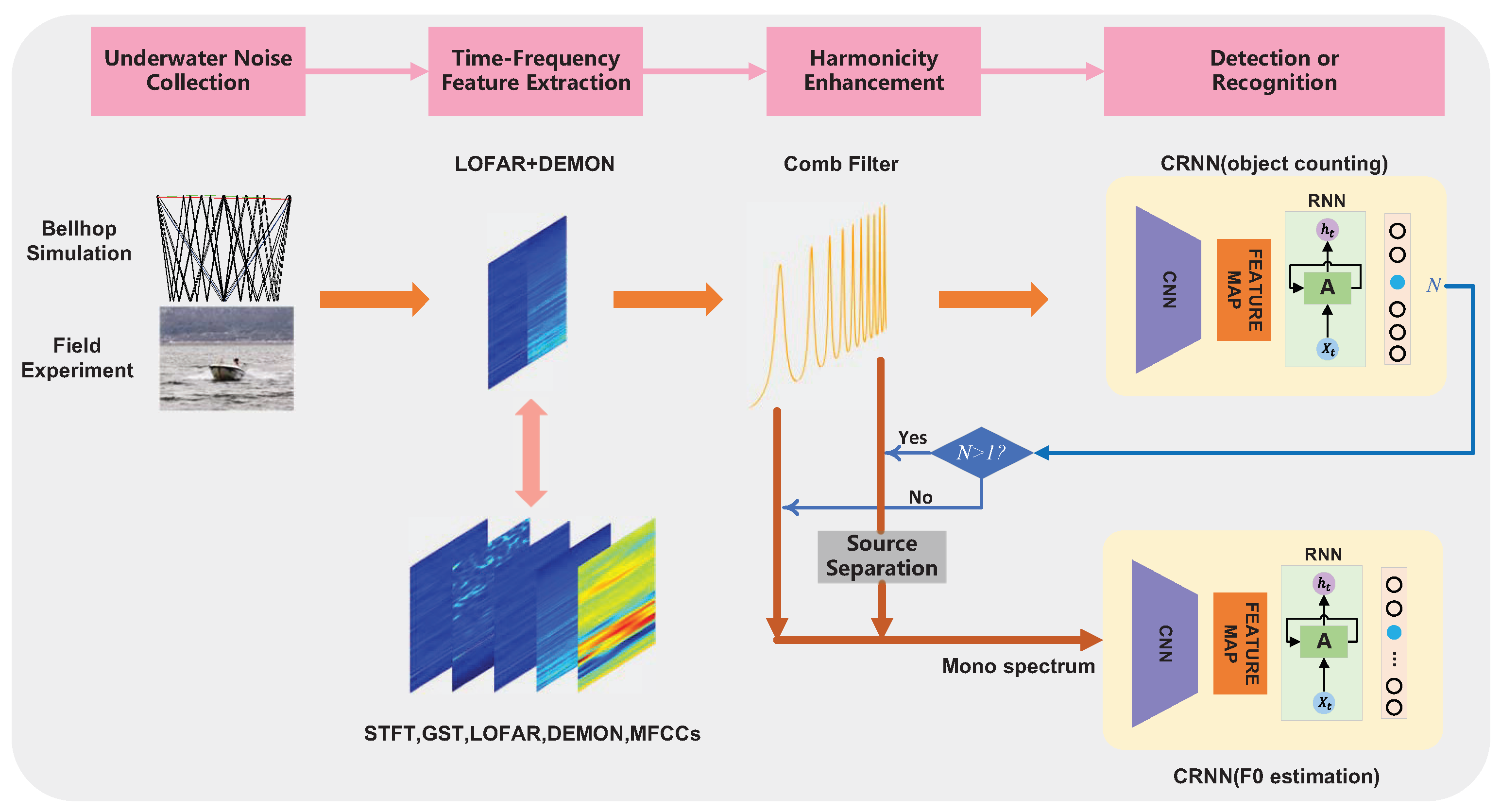
The proposed algorithm is composed of four steps, including radiated noise data acquisition, time-frequency feature extraction, harmonic enhancement, and CRNN-based object counting and F₀ estimation. Firstly, the radiated noises emitted by underwater acoustic targets are collected by the seabed or shore-based hydrophone, or the towed array or flank array carried by ship or AUV (single hydrophone towed by the mother ship in our experiment, see Section 3.2). Then, a time-frequency feature, which is the combination of LOFAR and DEMON and will be explained later in Section 2.1, is extracted from the incoming noise signal. For comparison, the traditional STFT, GST [32], LOFAR, DEMON, and MFCCs [33] are also extracted to predict the target number or F₀ in the experiment section. The feature combination of low-velocity compatible LOFAR and high-velocity compatible DEMON supports the radiated noise analysis in all working conditions. Due to the multi-path effects in underwater sound propagation and the disturbance from underwater ambient noise, the harmonic components of F₀ may be out of place, translated, weakened, broadened, or even distorted. Therefore, the comb filter is employed to enhance the harmonics and improve the quality of the time-frequency features. Finally, considering that the CRNN has become one of the standard tools for time series signal analysis and our main purpose is to optimize the feature extraction in detection and recognition tasks, we choose the basic CRNN as the classifier and do not modify the network structure in this paper. The proposed acoustic target detection system is displayed in Figure 1. The later three steps will be described in the following paragraphs, while the noise signal collection, including the noise simulation method, lake trial settings, and the corresponding noise datasets, will be presented in detail in Section 3 and Section 4.

2.1. Feature Extraction

2.1.1. Feature Combination

Radiated noise of underwater acoustic targets mainly includes the continuous spectrum, modulation spectrum, and line spectrum. A major source of continuous spectrum and modulation spectrum is cavitation noises, while the line spectrum and modulation spectrum are determined by the propeller rotations. The spectrum range to be analyzed should be carefully selected according to the relative intensity of each spectral component, which is largely related to the rotation speed of propellers.

• Low-speed case: With a low-speed rotation, the cavitation of the propeller is so weak that the peak of the continuous spectrum mainly lies on the high-frequency range. Therefore, the spectral lines are very prominent in the low-frequency range, and F₀ can be estimated directly by using the simple variants of STFT, such as the LOFAR spectrum. Please refer to [34] for a full introduction of LOFAR.
• High-speed case: With the increasing of rotation speed, the continuous spectrum grows rapidly, which reduces the comparative advantages of spectral lines to the continuous spectrum. On the other hand, the peak of the continuous spectrum gradually shifts to the low-frequency range, which further hinders the protrusion of spectral lines from the continuous spectrum. Fortunately, the periodic motion of the propeller has a very significant modulation effect on the strong high-frequency cavitation noises, from which the rotation parameters could be estimated confidently, such as in DEMON analysis. Please refer to [35] for an explicit description of DEMON.

It can be inferred from the above discussion that LOFAR and DEMON alone are unable to cope with arbitrary rotation speed estimation. In machine learning, the fusion of complementary features or classifiers helps improve the generalization ability of expert systems. Fusion can be accomplished at the feature level, for example, by concatenation, principal component analysis, and linear discriminant analysis, or the decision level, such as by Bayesian inference, Dempster–Shafer evidence theory, and so on [36]. Since both LOFAR and DEMON are time-frequency maps, we choose to concatenate them in the time dimension, which enriches the information of the feature without losing the physical attribution of both spectrums. Another reason for preferentially selecting feature-level fusion is that LOFAR and DEMON are appropriate for completely unrelated situations, which implies that only one estimation result is trustworthy, leading to the failure of decision-level fusion.

To demonstrate the speed selectivity of LOFAR and DEMON, two examples for the combined LOFAR + DEMON feature when the “Hailangdao” ship (see Section 3.2) moves with a lower rotation speed of 600 r·min${}^{-1}$ (F₀ = 10 Hz) and with a higher-rotation speed of 1200 r·min${}^{-1}$ (F₀ = 20 Hz) are given in Figure 2 and Figure 3, respectively, where LOFAR and DEMON are laying on the top and bottom panels, respectively. For the low-speed case in Figure 2, due to low-level cavitation, spectral lines in the LOFAR spectrum are very clear to identify, however, those in the DEMON spectrum are very hard to retrieve. The positions of spectral lines are A = 60 Hz, B = 90 Hz, C = 116 Hz (out of place), D = 150 Hz, and E = 180 Hz.

For the high-speed case in Figure 3, the positions of spectral lines are A1 = 120 Hz, A2 = 240 Hz, A3 = 360 Hz, B1 = 60 Hz, B2 = 120 Hz, B3 = 180 Hz, and B4 = 240 Hz. It can be seen that the spectral lines in LFOAR and DEMON satisfy the harmonic relationship approximately, however, on the other hand, not all the harmonics of the fundamental frequency are equally legible.

2.1.2. Availability of DEMON in the Case of Multiple Targets

To our knowledge, the DEMON spectrum has not been employed for object counting. When there are multiple targets, the continuous spectrum of each vehicle is modulated by the respective line spectrum. An additional cross-term will be introduced in the square step and may hinder the sequential demodulation step. Therefore, it is necessary to explain whether the DEMON spectrum is appropriate for the multiple-target case or not.

The radiated noise for a single target can be modeled by $s\left(t\right)=(1+m(t\left)\right)g\left(t\right)+l\left(t\right)$, where $m\left(t\right)$ represents the modulation spectrum, $g\left(t\right)$ for continuous spectrum and $l\left(t\right)$ for line spectrum, and $s\left(t\right)$ is the synthesized noise signal. Please refer to Section 3.1 for details.

According to square-law demodulation,

$$\begin{array}{cc}\hfill {\left(\sum _{i=1}^N{s}_i\left(t\right)\right)}^2& ={\left(\sum _{i=1}^N\left(1+m_i\left(t\right)\right)g_i\left(t\right)\right)}^2+2\sum _{i=1}^N\left(1+m_i\left(t\right)\right)g_i\left(t\right)\sum _{j=1}^N{l}_j\left(t\right)+{\left(\sum _{i=1}^N{l}_i\left(t\right)\right)}^2\hfill \\ \hfill & =\sum _{i=1}^N{\left(1+m_i\left(t\right)\right)}^2{g}_i^2\left(t\right)+\sum _{i=1,j=1,i\ne j}^N\left(1+m_i\left(t\right)\right)g_i\left(t\right)·\left(1+m_j\left(t\right)\right)g_j\left(t\right)\hfill \\ \hfill & +2\sum _{i=1}^N\left(1+m_i\left(t\right)\right)g_i\left(t\right)\sum _{j=1}^N{l}_j\left(t\right)+{\left(\sum _{i=1}^N{l}_i\left(t\right)\right)}^2\hfill \end{array}$$

(1)

where N is the target number and i for the ith target. Define

$$d_1\left(t\right)=\sum _{i=1}^N{\left(1+m_i\left(t\right)\right)}^2{g}_i^2\left(t\right),$$

(2)

$$d_2\left(t\right)=\sum _{i=1,j=1,i\ne j}^N\left(1+m_i\left(t\right)\right)g_i\left(t\right)·\left(1+m_j\left(t\right)\right)g_j\left(t\right),$$

(3)

$$d_3\left(t\right)=2\sum _{i=1}^N\left(1+m_i\left(t\right)\right)g_i\left(t\right)\sum _{j=1}^N{l}_j\left(t\right),$$

(4)

$$d_4\left(t\right)={\left(\sum _{i=1}^N{l}_i\left(t\right)\right)}^2.$$

(5)

Now, let us have a look at each term:

• $d_1\left(t\right)$
  Let $y_i\left(t\right)=g_i^2\left(t\right)$ and $z_i\left(t\right)={(1+m_i\left(t\right))}^2$, we have $d_{1i}\left(t\right)=y_i\left(t\right)z_i\left(t\right)$, and, in the frequency domain

  $$D_{1i}\left(f\right)=Y_i\left(f\right)\ast Z_i\left(f\right)$$

  (6)
  Because $z_i\left(t\right)$ is composed of Gaussian pulses with a fixed period ${\tau }_i$,

  $$z_i\left(t\right)=1+2\sum _n\frac{{\xi }_i}{\sqrt{2\pi }}{e}^{-\frac{{\left(t-n{\tau }_i\right)}^2}{2{\sigma }_i^2}}+\sum _n\frac{{\xi }_i^2}{2\pi }{e}^{-\frac{{\left(t-n{\tau }_i\right)}^2}{{\sigma }_i^2}},$$

  (7)

  its spectrum $Z_i\left(f\right)$ is also made up of a series of periodic pulses.
  According to [25], the power spectrum density (PSD) of $y_i\left(t\right)$ is $S_{y_i}\left(f\right)=R_G^2\left(0\right)\delta \left(f\right)+2S_G\left(f\right)\ast S_G\left(f\right)$, where $R_G\left(\tau \right)=E\left[g_i\left(t\right)g_i\left(t-\tau \right)\right]$ and $S_G$ is the PSD of $g_i\left(t\right)$.
  Note that $Y_i\left(f\right)$ has a relatively strong DC component and $Z_i\left(f\right)$ is composed of a series of impulses, thus, convolving $Z_i\left(f\right)$ with $Y_i\left(f\right)$ (refer to Equation (6)) leads to the enhancement of line spectrum. Therefore, the harmonic relationship is well preserved in $d_1\left(t\right)$.
• $d_2\left(t\right)$
  Take $d_2^{ij}\left(t\right)=\left(1+m_i\left(t\right)\right)g_i\left(t\right)·\left(1+m_j\left(t\right)\right)g_j\left(t\right)$, then $d_2^{ij}\left(t\right)=(1+m_i\left(t\right)+$
  $m_j\left(t\right)+m_i\left(t\right)m_j\left(t\right))g_i\left(t\right)g_j\left(t\right)$, where $m_i\left(t\right)$, $m_j\left(t\right)$ and $m_i\left(t\right)m_j\left(t\right)$ are periodic signals with periods of ${\tau }_i$, ${\tau }_j$, and ${\tau }_i{\tau }_j$, respectively. Let $m^{{}^{\prime }}\left(t\right)=m_i\left(t\right)+m_j\left(t\right)+m_i\left(t\right)m_j\left(t\right)$, spectral line structure in $m^{{}^{\prime }}\left(t\right)$ is dominated by the first two modulation terms because $m_i\left(t\right)m_j\left(t\right)$ can be treated as an additional modulation signal. Now that $g^{{}^{\prime }}\left(t\right)=g_i\left(t\right)g_j\left(t\right)$ is a continuous function, then $d_2^{ij}\left(t\right)=(1+m^{{}^{\prime }}\left(t\right))g^{{}^{\prime }}\left(t\right)$ can be seen as the assemble of the spectral lines of two targets (ith and jth). Therefore, the modulation spectrum structure of all targets is well preserved in $d_2\left(t\right)$.
• $d_3\left(t\right)$
  Take the Fourier transform of $d_3\left(t\right)$,

  $$D_3\left(f\right)\propto \sum _{i=1}^N{G}_i\left(f\right)\ast L\left(f\right)\ast M_i\left(f\right)\propto \sum _{i=1}^N{L}^{{}^{\prime }}\left(f\right)\ast M_i\left(f\right)$$

  (8)

  where the term irrelevant to the modulation spectrum $M_i\left(f\right)$ is omitted in the first approximation and the continuous spectrum $G_i\left(f\right)$ can be seen as the weight of line spectrum $L\left(f\right)$, where $L\left(f\right)={\sum }_{i=1}^N{L}_i\left(f\right)$. Therefore, the spectral lines are well preserved in $d_3\left(t\right)$
• $d_4\left(t\right)$
  $d_4\left(t\right)$ has nothing to do with the modulation spectrum.

In conclusion, the harmonic relationship underlying the modulation spectrum is well preserved in the square step, and the demodulation step could be carried out as usual.

2.2. Comb Filter

In a previous study [35], we employed the comb filter to enhance the harmonic relationship in the DEMON spectrum for the fundamental frequency estimation task based on multi-channel hydrophone data. In this paper, we further investigate its applicability in the combined LOFAR and DEMON features for the multiple-task mission, such as object counting and F₀ estimation.

For the ideal DEMON spectrum, the power distribution of F₀ and its harmonics in the logarithm frequency domain can be written as:

$$Y\left(q\right)=\sum _{k=1}^K{b}_k\delta (q-log\left(k\right)-log\left(F_0\right))+N\left(q\right)$$

(9)

where $q=logf$, k represents the order of harmonics and K for the total harmonic number. $N\left(q\right)$ represents the power spectral density of the unwanted noise and $b_k$ the power of the kth harmonic.

The comb filter can be regarded as a combination of many passbands and stopbands arranged with specific frequency intervals. Theoretically, the accumulation of harmonics in $Y\left(q\right)$ will result in a peak at $F_0$. The corresponding ideal comb filter in the logarithm frequency domain can be expressed as

$$h\left(q\right)=\sum _{k=1}^K\delta (q-log\left(k\right))$$

(10)

However, in practical engineering, the relationship between F₀ and its harmonics is not so strict that each impulse should cover a certain frequency width. As in [35], Equation (10) then turns to

$$h\left(q\right)=\left\{\begin{array}{cc}\hfill \frac{1}{\gamma -cos\left(2\pi e^q\right)}-\beta & ,log0.5<logq<logK+0.5,\hfill \\ \hfill 0& ,else.\hfill \end{array}\right.$$

(11)

where $\gamma$ represents the peak width and $\beta$ is designed so that $\int h\left(q\right)dq=0$

By removing the minus coefficients, the final comb filter could be written as

$$g\left(q\right)=\left\{\begin{array}{cc}\hfill h\left(q\right)& ,h\left(q\right)>0,\hfill \\ \hfill 0& ,else.\hfill \end{array}\right.$$

(12)

Finally, the enhanced DEMON spectrum as $Y^{{}^{\prime }}\left(q\right)$ is obtained by convolving the DEMON spectrum with the comb filtering

$$Y^{\prime }\left(q\right)=Y\left(q\right)\ast g(-q)$$

(13)

where ∗ represents the convolution operator.

In Figure 4, we display the enhanced version of the LOFAR + DEMON feature in Figure 3 after comb filtering. Since the energy of the line spectrum is mainly distributed in the low-frequency range, we take the logarithm of the frequency axis for easier visualization. Compared with the primitive combination spectrum, the low-frequency line spectrum becomes much more clear and prominent, and noisy spectral lines are suppressed in the filtering process. To some extent, the features are purified, the true but weak spectral lines are strengthened, while the false but strong spectral lines are filtered out.

2.3. Convolutional Recurrent Neural Network

Following our prior work in [7] and related works in the open literature [20,37], we treat in this paper the sound source counting and $F_0$ estimation as a classification problem. We denote the extracted feature of the radiated noise signal as S, we aim to find a mapping $h_w(·)$ that maps S to the number of sources n, $n\in {Z_0}^{+}$ or corresponding $F_0$ category. Without losing generality, the CRNN is employed to learn such a mapping. For a specific input S, $h_w\left(S\right)$ gives ($n_{max}+1$) posterior probability in the final full-connection layer with a softmax function $g(·)$. The category with the largest posterior probability corresponds to the number of sound sources or F₀.

The CRNN structure used in this paper is shown in Figure 5 and a summary of parameters in each layer is detailed in

Table 1. CRNN layers and hyperparameters.

Layer	Filters	Size	Input	Output
0    conv	16	$3\times 3/1$	$1\times 40\times 512$	$16\times 40\times 512$
1    batchnorm
2    maxpool		$2\times 2/2$	$16\times 40\times 512$	$16\times 20\times 256$
3    conv	1	$1\times 1/1$	$16\times 20\times 256$	$1\times 20\times 256$
4    batchnorm
6    fc	1	$c\times 160$	160	c
Layer	Input	Hidden Size		Output
5    lstm	$1\times 20\times 256$	8	160

. The output dimension, c, from the fc layer is adjusted according to the actual demand, such as the max target number $n_{max}$ or the number of $F_0$ classes. All hyperparameters are selected to achieve the best accuracy on the validation dataset. The CNN part consists of 16 convolution kernels with a size of $3\times 3$ and a pooling layer with a stride size of $2\times 2$, followed by a $1\times 1$ convolution. The output of CNN (with shape $20\times 256$ for the input of shape $40\times 512$) is fed to the LSTM network, followed by a fully connected layer, and finally passed through a softmax layer to get the output. The LSTM time step length is 20 and the number of layers is 1. Note that the maximum number of sources or rotation speed levels, $n_{max}$, needs to be prescribed in advance. In the later simulation experiments, the dimension of the final output one-hot vector is 6 and 12 in the object counting and F₀ estimation tasks, which corresponds to $0-5$ targets and 12 different rotation speeds, respectively.

A large amount of labeled data is required to train a deep network, which usually cannot be satisfied in many situations. The plan to collect underwater noise data is often daunted by the high experiment cost, which is further aggravated by the fact that it is very difficult for the human ear to capture gradual changes in rotation speed in the labeling stage. Therefore, the transfer learning strategy is adopted to train the CRNN, where the weights are firstly pre-trained by a large amount of simulation data, and then adjusted with a small amount of data collected in the lake trial by fine-tuning. Training was carried out on a computer with an Intel i7-10750 2.59 GHz CPU, 16 GB of RAM, and an NVIDIA RTX2060 GPU (1920 CUDA cores and 6 GB of RAM). We implemented a PyTorch version of our CRNN based on pytorch-1.9.0 and python 3.6.12

3. Dataset

The dataset used in this paper includes a simulation dataset and a lake trial dataset. The two major steps toward simulation data generation, including the sound source synthesis for the ship-radiated noise and the received signal simulation with Bellhop [38] model, will be briefly introduced in Section 3.1. Additionally, the lake trial dataset, which is mainly composed of ambient noise and radiation noise from tourist ships, will be introduced in Section 3.2.

3.1. Simulation Dataset

The spectrum of ship-radiated noise is mainly composed of the continuous spectrum, line spectrum, and modulation spectrum [39]. The time-domain waveform $s\left(t\right)$ can be described by [40]:

$$s\left(t\right)=(1+m(t\left)\right)g\left(t\right)+l\left(t\right)$$

(14)

where $g\left(t\right)$, $m\left(t\right)$, and $l\left(t\right)$ represent the continuous spectrum, modulation spectrum, and line spectrum component, respectively. The line spectrum is usually represented by a series of sine signals:

$$l\left(t\right)=\sum A_i\left(n\right)sin\left(2\pi (f_i/f_s)n+{\theta }_i\right)$$

(15)

where $A_i\left(n\right)$ is the amplitude factor, $f_i$ the line spectrum frequency, and $f_s$ the sampling frequency. The continuous spectrum is generated with the FIR filter which we have reported in early work, please refer to [35] for details. The modulation spectrum can be modeled by a series of normalized pulses with random amplitudes, shapes, and periods,

$${\mu }_{\xi }\left(t\right)=\frac{\xi }{\sqrt{2\pi }}exp\left[-t^2/\left(2{\sigma }^2\right)\right]$$

(16)

where $\xi$ represents the random perturbations in pulse amplitude and $\sigma$ the pulse width.

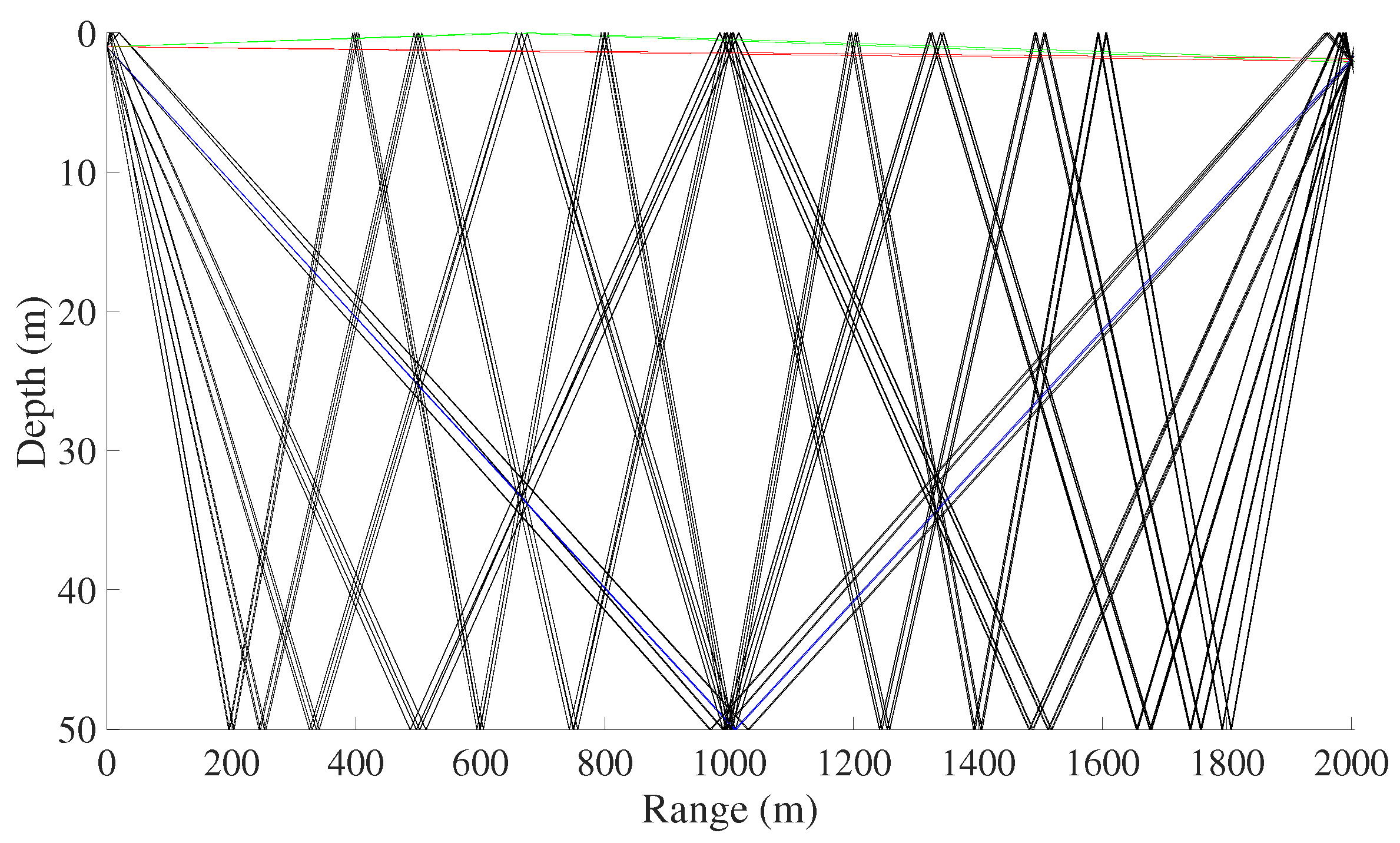
To validate the transfer learning and approach the real noise dataset by the simulation data with the same marginal probability distribution, it is preferred to model the underwater sound propagation process when simulating the received signal, including the average propagation loss of sound energy, the multipath interference caused by the reflection from the seabed and the sea surface, and the additive interference of marine environmental noise. The Bellhop toolkit, which is based on the ray acoustic theory, is adopted to simulate propagation loss and multi-path interference. It employs Gaussian beam tracing to compute the acoustic fields underwater in a cylindrical coordinate system. Compared with traditional ray-tracing methods, the Gaussian beam tracing can get rid of certain ray-tracing artifacts such as perfect shadows and infinitely high energy at caustic. More precisely, the central ray of Gaussian beams is firstly constructed with the integration of the usual ray equations, and then a pair of auxiliary equations governing the evolution of the beam is integrated about the rays to generate beams, resulting in a pressure field that falls off in a Gaussian fashion as a function of normal distance from the central ray of the beam [38]. The hydrophone and multiple sound sources are firstly placed at the given positions. For every single source, the unit impulse response of the transmission channel between the source and hydrophone is calculated, which is then convolved with the simulated noise to obtain the received signal at the hydrophone. We implemented the Bellhop simulation with Matlab R2021a and bellhop toolkit 2020 1. The distance between the sound source and the hydrophone is set to be 2 km, which is equal to the maximum distance between the target ship and the receiving hydrophone in the lake trial. Further, we add Gaussian white noises to the received signal with $SNR$ = 43 dB.

An example of the sound eigenray diagram of a single source during simulation is shown in Figure 6. Since the radiated noise of a ship is mainly from the propeller, the sound source depth here is set to approximate the real ship’s propeller depth, $d_S$ = 1.0 m. The hydrophone is deployed below the water surface with a depth of $d_H$ = 2.0 m, the water depth is 50 m, the bottom condition is assumed to be approximately flat, and the sound speed is constant at 1500 m·s${}^{-1}$.

For the target counting task, the simulation parameters setting is as follows: the radiated noise of a single source follows the distribution depicted in Equation (14) and lasts for 1 s. When there are multiple sources, the received signals for each source are simulated individually and summed up as the final output. In the simulation, target number $N\in [0,5]$, blade number $N_{blades}\in \{3,4,5,7\}$, the rotation speed of propeller lies between 480 and 1500 r·min${}^{-1}$, and the sampling frequency is $Fs$ = 10 kHz. In total, 2 h of simulation noise is generated to train the network for object counting.

For the F₀ estimation task, only a single source with different rotation speeds is simulated to generate the dataset. Note that, again, source separation is needed in the case of multiple sources [6], and it is not discussed in this paper. The depth of the sound source and hydrophone is the same as that in target counting. Simulation dataset for F₀ estimation consists of synthesized noise radiated from a single source, where the rotation speed $R_p\in \{8,9,10,11,12,13,14,15,16,17,18,19\}$ and the number of blades is chosen randomly from $\{3,4,5,7\}$. For each selected rotation speed and blade number, 200 noises data samples with length 1 s are generated, and the final F₀ estimation dataset has a total time length of about 3 h.

Figure 7 compares the spectrum of the simulated ship noise signal before and after the Bellhop simulation. The overall transmission loss is about 70 dB, which is clearly shown on the spectrum. Additionally, as stated in Figure 7, part of the line spectrum (line spectrum at 30 Hz) is distorted during the sound propagation.

3.2. Lake Trial Dataset

To test the algorithm, we conducted a lake trial in Songhua Lake, Jilin City, Jilin Province in November 2021. During the experiment, a hydrophone was deployed on an anchored mother ship, and the target ship moved at a uniform speed in front of the mother ship along a planned line trajectory, from left to right, back and forth. The sound source level for the target ship was about 130 dB, while that of in-site ambient noise was about 102 dB. The targets include three four-blade tourist ships and a three-blade yacht. The basic information about ships used in the experiment is listed in

Table 2. Information of ships in the lake trial.

Notation	Tonnage (t)	${\mathit{N}}_{\mathit{blades}}$	Rotation ($\times {10}^3$ r·min${}^{-1}$)
Wanbang	81	4	$\{1.0,1.2,1.4\}$
Hailangdao	39	4	$\{1.0,1.2,1.4\}$
Tuolun	21	4	$\{0.7,0.8,0.9,1.0,1.1\}$
Motorboat	<1	3	$\{1.0,1.5,2.0,2.5,3.0,3.5,4.0,4.5,5.0\}$

. For data collection, two types of hydrophones were employed during the lake trial. The first one is an omnidirectional hydrophone with a sensitivity of $-172dBVre\mu Pa$ connected to a data acquisition board integrated with an amplifier ($\times 100$ or $\times 1000$) and a band-pass filter whose pass-band lies in 100 Hz∼20 kHz. The sampling rate is $10\mathrm{kHz}$. An Ethernet link is established to transfer the data from the board to the laptop. The second one is a smart hydrophone of the icListen series modeled SC2-X2 and manufactured by Ocean Sonic, working with a sample rate of 48 kHz.

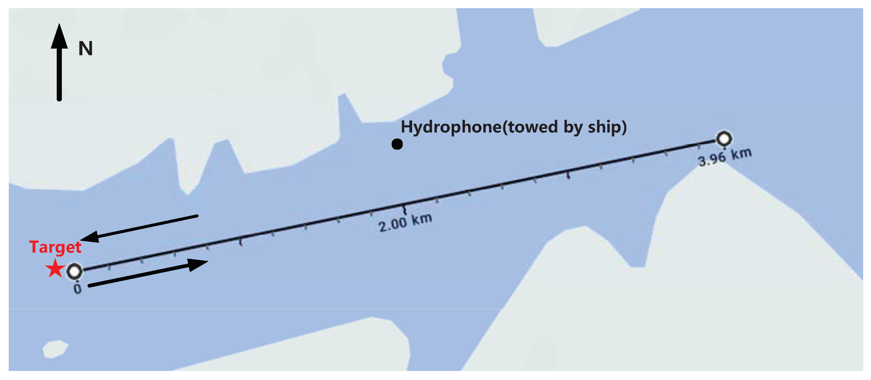
The geographic environment and the motion trajectory are shown in Figure 8. When collecting the noise data of a single target, the mother ship that carries the hydrophone is anchored. The hydrophone depth is about 2 m from the water surface. The target ship moves along the marked trajectory (solid black line) back and forth at different speeds, however, the velocity is fixed for each voyage. When collecting the noise of two targets, the mother ship also acts as a noise source and moves along a trajectory that is approximately parallel to the trajectory of the first target, however, with a different speed.

4. Experiment

Four experiments were designed to evaluate the feasibility of the proposed feature combination strategy and comb filtering in object counting and F₀ estimation tasks.

• Object counting: Evaluate and compare the performance of different features on the simulation dataset when feeding into the CRNN, including STFT, GST, LOFAR, DEMON, MFCCs, and the proposed LOFAR + DEMON;
• F₀estimation: The experiment setting is the same as in exp. 1, except with a different output layer;
• Comb filtering: Apply the comb filtering to the features extracted in exp. 1 and retrain the classification network for object counting and F₀ estimation. Then, compare the prediction accuracy of each feature before and after the comb filtering;
• Lake trial: Feed the features of real noise data collected in the lake trial into the CRNN and test their performance in practical object counting and F₀ estimation tasks.

4.1. Metrics for Evaluation

In this paper, the object counting and recognition are treated as classification tasks. Therefore, evaluation metrics in multi-classification tasks are selected, including accuracy, precision, recall, and F₁ score. Among them, the accuracy describes the performance of the algorithm on the total dataset, while the precision, recall, and F₁ score are used to evaluate the actual performance of the algorithm in a certain category. Metrics are defined as follows:

$$Accuracy=\frac{TP+TN}{TP+TN+FP+FN}$$

(17)

$$Precision=\frac{TP}{TP+FP}$$

(18)

$$Recall=\frac{TP}{TP+FN}$$

(19)

$$F_1=\frac{2}{Precisio{n}^{-1}+Recal{l}^{-1}}=2\times \frac{Precision\times Recall}{Precision+Recall}$$

(20)

where TP, TN, FP, and FN represent the true positive, true negative, false positive, and false negative, respectively.

4.2. Object Counting

Precise target number estimation is the premise of subsequent semantic analysis, such as sound source separation, target recognition, and so on. This experiment is mainly devoted to comparing the performance of each feature (comb filtering excluded) in the target counting task on the simulation dataset.

In extracting the time-frequency features, the window length is set to be $wi{n}_{len}=5000$, and two neighboring frames have a hop length of 125 samples. With STFT, GST, LOFAR, and DEMON, only the spectrum over $f\in [0,1024)$ Hz is reserved, since the high-frequency part contains less information, leading to a feature matrix with dimensions of $40\times 512$. With MFCCs, the full spectrum is used to calculate the cepstrum coefficients and the final feature matrix is in shape $40\times 39$.

For the object counting task in the simulation condition, the output dimension of our network is $c=6$, since we have $n_{max}=5$. About 80% of the dataset is for training, while the remaining is for validation. The initial learning rate is $lr=3\times {10}^{-4}$, the mini-batch size is set to be 16, and the SGD optimizer is adopted to optimize the parameters in the network.

In

Table 3. Performance of each feature when feeding into the CRNN for object counting on the simulation dataset (COMB excluded).

Features	Accuracy
MFCCs	37%
LOFAR	79%
DEMON	80%
GST	84%
STFT	87%
LOFAR + DEMON (Ours)	87%

, we list the performance of each feature in the object counting task on the simulation dataset. Several conclusions can be drawn: (1) STFT and the proposed LOFAR + DEMON feature have the highest estimation accuracy, which is consistent with the finding in [20] that the STFT feature achieves the minimum MAE in speaker count. (2) LOFAR or DEMON alone have moderate performance in the counting task, while GST has a slightly better estimation accuracy. Since LOFAR is a simple variant of STFT, it demonstrates that the removing tendency in STFT is prone to cause information loss. (3) MFCCs feature has relatively poor results compared with the other features, which also supports the conclusion in [41] that MFCCs showed poor performance when feeding into the CNNs.

4.3. F₀ Estimation

The ultimate goal of target detection is object recognition and parameter estimation. If the features extracted for counting could be shared by later-stage F₀ estimation, it will save large amounts of computational resources.

When there are multiple sources, the mixture noises should be separated into components. In [6], we have successfully separated two noises using the U-Net network. Inspired by [42], we are trying to extend it to more complex cases using deep-clustering, which will be present in a future report. In this paper, only the efficiency of the feature is concentrated, and we directly extract features from each single source signal and feed them into the CRNN for F₀ estimation. The experiment settings for F₀ estimation is the same as that in Section 4.2 except that the dimension of final output is 12, refer to Section 3.1 for details of simulation dataset.

The training curve for each feature in the F₀ estimation task on the simulation dataset is shown in Figure 9, and the final prediction accuracy of different features is listed in

Table 4. Performance of each feature when feeding into the CRNN for F₀ estimation on the simulation dataset (COMB excluded).

Features	Accuracy
MFCCs	10%
DEMON	92%
GST	98%
STFT	99%
LOFAR	99%
LOFAR + DEMON (Ours)	100%

.

It can be seen that all the features except MFCCs have achieved satisfactory results in the F₀ estimation task. In terms of accuracy, the proposed LOFAR + DEMON feature is comparable to STFT and LOFAR. The convergence speed of the GST feature and DEMON feature is relatively slow, and the accuracy of the DEMON feature is slightly lower than that of the GST feature.

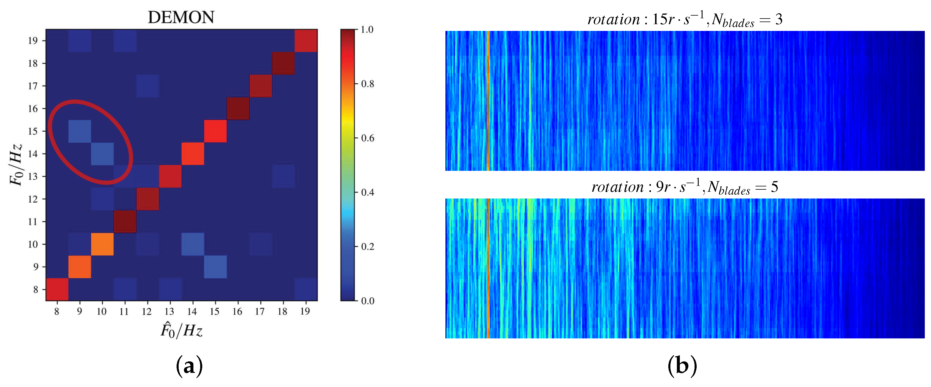
To further explore the factors that affect the prediction performance of the DEMON spectrum, the confusion matrix for all fundamental frequencies is presented in Figure 10a, with the two classes with the largest errors annotated by a red circle. Theoretically, the DEMON spectrum of a signal generated by a three-blade propeller rotating with a speed of $15\mathrm{r}·{\mathrm{s}}^{-1}$ is very similar to that of the signal generated by a five-blade propeller rotating with a speed of $9\mathrm{r}·{\mathrm{s}}^{-1}$. Equal blade frequency brings a great challenge for the DEMON-based algorithm, see Figure 10b for reference. Other estimation errors could be explained similarly. Note that MFCCs fail in the recognition task since no fundamental frequency information can be directly derived from an MFCC feature map.

4.4. Comb Filtering

It is assumed in Section 3.2 that, theoretically, the comb filter is helpful for enhancing the harmonicity between F₀ and its harmonics. To test this hypothesis, we apply it to the extracted time-frequency spectrum in Section 4.2 and Section 4.3, and feed the filtered feature into the CRNN. Except for the addition of a comb filtering block, all the other experiment settings are kept the same as before. Note that no harmonicity can be found in MFCCs, therefore, comb filtering is not applied to MFCCs.

4.4.1. Target Counting

The prediction accuracy for target counting is presented in

Table 5. Performance of each feature when feeding into CRNN for object counting on the simulation dataset (COMB included).

Features	Accuracy
LOFAR + COMB	65%
DEMON + COMB	68%
STFT + COMB	70%
GST + COMB	77%
LOFAR + DEMON + COMB (Ours)	72%

. Compared with Table 3, it is astonishing to find that the prediction accuracy of the CRNN when the comb filter is applied to the time-frequency spectrum turns out to have deteriorated, which is fully contrary to our expectation. To explore the reasons underlying these curious phenomena, we compare the feature spectrum before and after comb filtering, and find that the spectral lines become much denser in the case of multiple objects, however, the gaps between closing spectral lines become blurred and indistinct after filtering due to the broadband effects from comb filtering. Therefore, it could be concluded that comb filtering is inappropriate for underwater noise target counting tasks.

4.4.2. F₀ Estimation

The prediction accuracy, in addition to the convergence speed (epochs needed to achieve 95% accuracy), for F₀ estimation is listed in

Table 6. Prediction accuracy and convergence speed of each feature when comb filtering is included or not, based on features before and after enhancement, L + D is the abbr. of LOFAR + DEMON. Changes in accuracy and convergence speed are highlighted in bold format.

Features	Accuracy	Epochs to Converge
DEMON	92%	80
DEMON + COMB	92%	60 $(\downarrow )$
GST	98%	140
GST + COMB	99% $(\uparrow )$	20 $(\downarrow )$
LOFAR	99%	10
LOFAR + COMB	96% $(\downarrow )$	10
STFT	99%	15
STFT + COMB	99%	15
L + D (Ours)	100%	40
L + D + COMB (Ours)	100%	20 $(\downarrow )$

. For easier understanding, the training process is displayed in Figure 11. Several conclusions may be drawn: (1) the prediction accuracy is almost unchanged after the employment of comb filtering, partly due to the fact that the SNR of spectral lines is already very high in the simulation dataset that comb filtering is unable to further improve the prediction performance. (2) The convergence speed is significantly accelerated for DEMON, GST, and LOFAR + DEMON features, which indirectly indicates that comb filtering is beneficial for feature enhancement, facilitating the deep learning network quickly capturing the harmonics underlying the time-frequency spectrum during the training process.

It is worth noting that the performance of LOFAR + COMB is inferior to LOFAR in F₀ estimation. In

Table 7. Evaluation metrics for LOFAR + COMB when feeding into the CRNN for F₀ estimation on the simulation dataset, two pairs of rotations with integral multiplication relationship are highlighted in bold format.

Rotation (r·s−1)	Precision	Recall	F1 Score
08	95%	92%	94%
09	92%	89%	91%
10	100%	96%	98%
11	100%	100%	99%
12	100%	92%	96%
13	100%	100%	100%
14	100%	100%	100%
15	94%	100%	97%
16	94%	98%	96%
17	100%	97%	99%
18	88%	91%	89%
19	95%	100%	97%

, we provide the precision, recall, and F₁ score of the LOFAR + COMB feature on various rotation speeds on the test dataset. It can be seen that the algorithm degrades when one category is the integral multiplication of another one, as shown in Table 7 (in bold format). For example, when the comb filtering is employed, the LOFAR + COMB spectrums corresponding to the situations when the rotation speed is 8 r·s${}^{-1}$ or 16 r·s${}^{-1}$ are very similar to each other, leading to estimation failures.

4.5. Performance on the Lake Trial Dataset

It can be concluded from the above experiments in Section 4.2, Section 4.3 and Section 4.4 that with the simulation dataset, LOFAR + DEMON achieves the highest counting accuracy, while LOFAR + DEMON + COMB has the best performance in F₀ estimation. However, no matter the target noise model or the sound transmission channel, the practical underwater environment is far more complex than the simulation settings.

Therefore, it is necessary to check if the conclusions hold true in real underwater environments. The experiment settings for lake trial noise data collection have already been described in Section 3.2. Target counting datasets include environmental noise, single-target noise data, and two-target mixed noise. The F₀ estimation dataset is from single-target radiated noise data with rotational speeds including $\{700,800,900,1000,1100,1200,1400\}$ r·min${}^{-1}$.

4.5.1. Target Counting

The lake trial dataset used for target counting has a total of 5224 noise signal segments with a length of 1 s. On the basis of network weights in Section 4.2, we use a small proportion of lake trial data, about 10%, to fine-tune the network parameters after replacing the final fully connected (FC) layer, and test its classification accuracy on the remaining target counting dataset. The prediction accuracy is listed in

Table 8. Performance of the algorithm based on different features on the lake trial dataset in object counting task (COMB excluded).

Features	Accuracy
STFT	87%
GST	89%
LOFAR	96%
DEMON	97%
LOFAR + DEMON (Ours)	100%

. Since the number of targets is not more than two, the proposed LOFAR + DEMON spectrum achieved an accuracy of 100% by no accident. Furthermore, it is superior to all the other features, which is consistent with the simulation dataset.

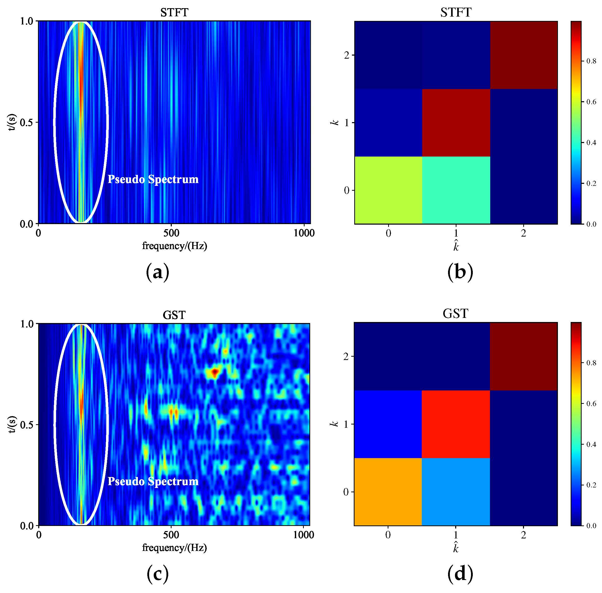
Compared with the results on the simulation dataset, the counting accuracy of LOFAR or DEMON alone is slightly inferior to that of the combined LOFAR + DEMON spectrum, however, STFT and GST dropped sharply. The reason that either LOFAR or DEMON has a better performance in the real dataset is that the target number is far less than that in the simulation dataset. Part data samples are collected with a hydrophone with strong electrical noises, which introduces pseudo-lines that are very similar to the spectral lines into the feature spectrum. Refer to Figure 12a,c for an example. The confusion matrix when STFT or GST is employed is shown in Figure 12b,d, respectively, which demonstrates, again, that the prediction error is mainly from the confusion in electrical noise and single-target noise. LOFAR can cope with the disturbance brought in by the strong electrical noise to a certain extent, mainly owing to the frame power normalization. For DEMON, no modulation occurs when there is no target, while in a single target condition, the demodulation is effective when the target is sailing with a high speed, enabling the successful classification of zero target and single-target condition.

4.5.2. F₀ Estimation

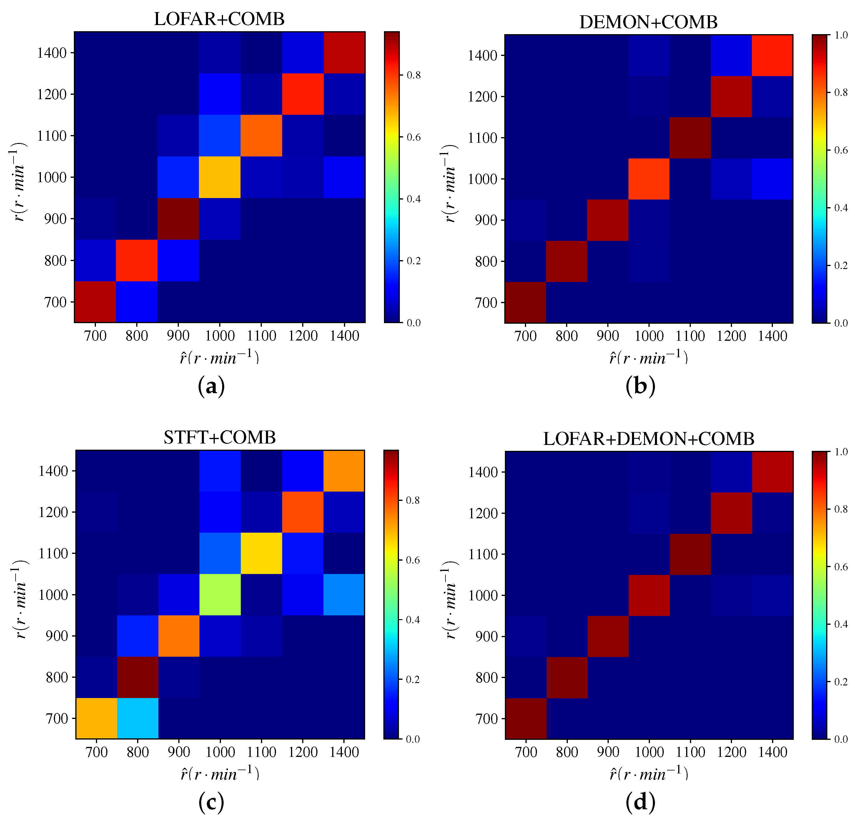
The lake trial dataset used for F₀ estimation has a total of 1665 noise segments with lengths of 1 s. On the basis of Section 4.3, we also use 10% of the lake trial data to fine-tune the network weights after the replacement of the classification head, and test its classification accuracy on the remaining data samples. With respect to the moderate performance of MFCCs on the simulated dataset, it is abandoned in analyzing the real dataset. The prediction accuracy is listed in

Table 9. Performance of algorithm based on different features on the lake trial dataset in F₀ estimation task (COMB included).

Features	Accuracy
GST + COMB	74%
STFT + COMB	74%
LOFAR + COMB	83%
DEMON + COMB	94%
LOFAR + DEMON + COMB (Ours)	98%

. The proposed LOFAR + DEMON + COMB strategy achieves 98% accuracy (Figure 13d), and is superior to other features, which is consistent with the conclusions drawn from the simulation dataset. It should be mentioned that the lake trial dataset has been filtered by a band-pass filter whose passband lies in 100–20,000 Hz. Therefore, the estimation accuracy of STFT, GST, and LOFAR combined with comb filter drops to different extents, as illustrated in Table 9.

The confusion matrices for STFT+COMB, LOFAR + COMB, DEMON + COMB, and LOFAR + DEMON + COMB are presented in Figure 13. LOFAR is different from STFT by the addition of TPSW filtering, where the removal of the trend term highlights the spectral lines, improving the discriminability of the feature spectrum (Figure 13a,c). However, it is somewhat difficult to infer rotation speed from the LOFAR + COMB spectrum. Comparatively, DEMON has relatively better performance in all categories (Figure 13b).

5. Conclusions and Discussion

There are several tasks included in a typical underwater multi-target detection mission, such as object counting, source separation, motion parameter estimation, object recognition, and so on. In these multi-task situations, it is hoped to extract reusable features as much as possible and feed them into classifiers with the same structure to complete different tasks. In this paper, we consider two typical tasks, target counting and F₀ estimation, and propose the combined LOFAR + DEMON spectrum and the comb filtering strategy to extract the feature in the framework of deep learning, with a standard CRNN adopted as the classifier. The feasibility of the proposed fusion feature is verified through simulation and lake trial experiments. Conclusions are as follows: (1) the combined feature LOFAR + DEMON has the best prediction accuracy in both target counting and F₀ estimation tasks. (2) Comb filtering is beneficial for F₀ estimation; however, it is not suitable for target counting. (3) The inclusion of comb filtering largely accelerates the convergence speed for the training process in the F₀ estimation task.

The performance of an underwater acoustic target detection system not only is determined by the speed, working condition, and mechanical characteristics of the target, but is also dependent on the hydrological environment, and the relative position between the sound source and target. The underwater acoustic channel propagation characteristics and time-varying sound field will have huge impacts on the radiation noise, especially when the hydrophone lies in the shadow area, which is, however, beyond the scope of this research. Therefore, in this paper, there is a basic assumption: the hydrophone can receive the radiation noise from the target. On this basis, the relationship between working conditions and radiation noise, as well as the extraction of a general time-frequency feature are investigated.

The target type, such as surface or underwater target, the target size, and the target speed will have a great impact on the sound level of radiation noise. For example, the sound level of a large surface ship even exceeds 200 dB, while that of some submarines has been lower than 100 dB. In the lake trial carried out in this paper, the sound source level is about 130 dB when the ship traveled at 8 knots. It demonstrates that different targets have completely different radiation noise characteristics, which requires the detection system to have a good generalization ability. Different from the sound intensity, which strongly depends on the target size, the line spectrum is mainly determined by the velocity and has been widely adopted to detect underwater acoustic targets. The feature extraction strategies in this paper also belong to this framework, with a focus on how to extract a relatively universal feature in different working conditions.

During the propagation of radiation noise, the signal attenuation and scattering as well as the superposition of ambient noise will reduce the SNR of the source signal, greatly challenging the target detection and recognition missions. Specifically, the spectral lines implied in LOFAR and DEMON spectrums will become more and more ambiguous, which largely discounts the traditional classifiers that strongly depend on the feature structures. To better evaluate features and reduce the coupling between features and classifiers as much as possible, we employ the CRNN, whose generalization performance has been widely appreciated in speech or noise analysis, as the common classifier. It should be noted that whether model-driven or data-driven, a trained classifier will be faced with environmental adaptability problems when applied to actual platforms or projects, no less when talking about the time-varying marine environment. Therefore, it is necessary to accumulate a large amount of hydrological data and improve the feasibility of simulation data through data modeling, on the one hand, and collect as much practical data as possible to improve the generalization ability and reliability of the detection system on the other hand.

The target number, implemented by the target counting network could be used to guide the late-stage source separation. Currently, we are trying to separate multiple sources when the target number exceeds two. Therefore, in the near future, we will combine the source separation algorithm with the target counting network and the F₀ estimation network developed in this paper into an integrated system. On the other hand, we will try to share the network weights between the target counting network and the F₀ estimation network, so that the memory and computation cost could be largely reduced. Moreover, it is noticeable that the classifier with meta-heuristic optimizer is getting more and more attention in the open literature [43,44] due to the local minima avoidance ability, which might be an alternative for our CRNN.

References

1. Cheng, Y.; Qiu, J.; Liu, Z. Challenges and prospects of underwater acoustic passive target recognition technology. J. Appl. Acoust. 2019, 38, 653–659. (In Chinese) [Google Scholar] [CrossRef]
2. Wang, L.; Wang, Y.; Song, S.; Li, F. Overview of fibre optic sensing technology in the field of physical ocean observation. Front. Phys. 2021, 9, 745487. [Google Scholar] [CrossRef]
3. Mirzaei, S.; Van Hamme, H.; Norouzi, Y. Blind audio source counting and separation of anechoic mixtures using the multichannel complex NMF framework. Signal Process. 2015, 115, 27–37. [Google Scholar] [CrossRef] [Green Version]
4. He, H.; Cang, Y. The Application Research of Underwater Acoustic Source Numbers Estimation by Blind Separation Algorithm. In Proceedings of the 2009 International Conference on Computational Intelligence and Software Engineering, Wuhan, China, 11–13 December 2009; pp. 1–4. [Google Scholar] [CrossRef]
5. Yamamoto, K.; Asano, F.; Van Rooijen, W.; Ling, E.; Yamada, T.; Kitawaki, N. Estimation of the number of sound sources using support vector machines and its application to sound source separation. In Proceedings of the 2003 IEEE International Conference on Acoustics, Speech, and Signal Processing (ICASSP), Hong Kong, China, 6–10 April 2003; Volume 5, p. V-485. [Google Scholar] [CrossRef]
6. Li, L.; Zhang, W.; Ji, Z.; Jing, Y.; Pang, G.; Wang, L.; Song, S. Self-noise Removal Using U-Net for AUV-based Underwater Target Detection. Digit. Ocean Underw. Warf. 2021, 4, 446–452. (In Chinese) [Google Scholar] [CrossRef]
7. Lu, J.; Song, S.; Jing, Y.; Zhang, Y.; Gu, L.; Lu, F.; Hu, Z.; Li, S. Fundamental frequency detection of underwater target noises using DEMON spectrum and LSTM network. Appl. Acoust. 2021, 40, 745–753. (In Chinese) [Google Scholar] [CrossRef]
8. Nielsen, R. Cramer-Rao lower bounds for sonar broad-band modulation parameters. IEEE J. Ocean. Eng. 1999, 24, 285–290. [Google Scholar] [CrossRef]
9. Cohen, L. Time-frequency distributions-a review. Proc. IEEE 1989, 77, 941–981. [Google Scholar] [CrossRef] [Green Version]
10. Nielsen, R. Sonar Signal Processing; Artech House Inc.: Nortwood, MA, USA, 1991. [Google Scholar]
11. Fernandes, J.d.C.V.; de Moura Junior, N.N.; de Seixas, J.M. Deep Learning Models for Passive Sonar Signal Classification of Military Data. Remote Sens. 2022, 14, 2648. [Google Scholar] [CrossRef]
12. Akaike, H. A New Look at the Statistical Model Identification; Springer: New York, NY, USA, 1974; Volume 19, pp. 215–222. [Google Scholar] [CrossRef]
13. Rissanen, J. Modeling by shortest data description. Automatica 1978, 14, 465–471. [Google Scholar] [CrossRef]
14. Hannan, E.; Quinn, B. The Determination of the Order of an Autoregression. J. R. Stat. Soc. Ser. B Methodol. 1979, 41, 190–195. [Google Scholar] [CrossRef]
15. Wu, H.T.; Yang, J.F.; Chen, F.K. Source number estimators using transformed Gerschgorin radii. IEEE Trans. Signal Process. 1995, 43, 1325–1333. [Google Scholar] [CrossRef]
16. Sun, L.; Cheng, Q. Indoor sound source localization and number estimation using infinite Gaussian mixture models. In Proceedings of the 2014 48th Asilomar Conference on Signals, Systems and Computers, Pacific Grove, CA, USA, 2–5 November 2014; pp. 1189–1193. [Google Scholar] [CrossRef]
17. Nguyen, T.; Gan, W.S.; Ranjan, R.; Jones, D. Robust Source Counting and DOA Estimation Using Spatial Pseudo-Spectrum and Convolutional Neural Network. IEEE/ACM Trans. Audio Speech Lang. Process. 2020, 28, 2626–2637. [Google Scholar] [CrossRef]
18. Yang, Y.; Gao, F.; Qian, C.; Liao, G. Model-Aided Deep Neural Network for Source Number Detection. IEEE Signal Process. Lett. 2020, 27, 91–95. [Google Scholar] [CrossRef] [Green Version]
19. Stoter, F.R.; Chakrabarty, S.; Edler, B.; Habets, E. Classification vs. Regression in Supervised Learning for Single Channel Speaker Count Estimation. In Proceedings of the 2018 IEEE International Conference on Acoustics, Speech and Signal Processing (ICASSP), Calgary, AB, Canada, 15–20 April 2018; pp. 436–440. [Google Scholar] [CrossRef] [Green Version]
20. Stoter, F.R.; Chakrabarty, S.; Edler, B.; Habets, E. CountNet: Estimating the Number of Concurrent Speakers Using Supervised Learning. IEEE/ACM Trans. Audio Speech Lang. Process. 2018, 27, 268–282. [Google Scholar] [CrossRef] [Green Version]
21. Yaman, O.; Tuncer, T.; Tasar, B. DES-Pat: A novel DES pattern-based propeller recognition method using underwater acoustical sounds. Appl. Acoust. 2021, 175, 107859. [Google Scholar] [CrossRef]
22. Yin, J.; Hui, J.; Yao, Z. Extraction of shaft frequency based on the DEMON line spectrum. Appl. Acoust. 2005, 24, 369–374. (In Chinese) [Google Scholar] [CrossRef]
23. Fang, N.; Juan, H.; Huachao, C.; Haixu, D.; Mengxiao, Y. Sea trial researches on extraction of propeller shaft frequency. In Proceedings of the Proceedings 2013 International Conference on Mechatronic Sciences, Electric Engineering and Computer (MEC), Shenyang, China, 20–22 December 2013; pp. 1306–1309. [Google Scholar] [CrossRef]
24. Yang, R.; Zheng, X.; Han, J. An automatic extraction method of propeller shaft frequency based on sequence matching. Vib. Shock 2018, 37, 57–61. (In Chinese) [Google Scholar]
25. Rao, B. Feature Extraction Method for Weak Modulation of Ship Radiated Noise. Master’s Thesis, Southeast University, Dhaka, Bangladesh, 2019. (In Chinese). [Google Scholar]
26. Neupane, D.; Seok, J. A Review on Deep Learning-Based Approaches for Automatic Sonar Target Recognition. Electronics 2020, 9, 1972. [Google Scholar] [CrossRef]
27. Jansson, A.; Bittner, R.; Ewert, S.; Weyde, T. Joint Singing Voice Separation and F0 Estimation with Deep U-Net Architectures. In Proceedings of the 2019 27th European Signal Processing Conference (EUSIPCO), A Coruna, Spain, 2–6 September 2019; pp. 1–5. [Google Scholar] [CrossRef] [Green Version]
28. Bittner, R.M.; McFee, B.; Salamon, J.; Li, P.; Bello, J.P. Deep Salience Representations for F0 Estimation in Polyphonic Music. In Proceedings of the 18th International Society for Music Information Retrieval Conference (ISMIR 2017), Suzhou, China, 23–27 October 2017; pp. 63–70. [Google Scholar]
29. Kim, J.; Salamon, J.; Li, P.; Bello, J. Crepe: A Convolutional Representation for Pitch Estimation. In Proceedings of the 2018 IEEE International Conference on Acoustics, Speech and Signal Processing (ICASSP), Calgary, AB, Canada, 15–20 April 2018; pp. 161–165. [Google Scholar] [CrossRef] [Green Version]
30. Gonzalez, S.; Brookes, M. PEFAC—A Pitch Estimation Algorithm Robust to High Levels of Noise. IEEE/ACM Trans. Audio Speech Lang. Process. 2014, 22, 518–530. [Google Scholar] [CrossRef]
31. Valin, J.M. A hybrid DSP/deep learning approach to real-time full-band speech enhancement. In Proceedings of the 2018 IEEE 20th International Workshop on Multimedia Signal Processing (MMSP), Vancouver, BC, Canada, 29–31 August 2018; pp. 1–5. [Google Scholar] [CrossRef] [Green Version]
32. Stockwell, R.; Mansinha, L.; Lowe, R. Localization of the complex spectrum: The S transform. IEEE Trans. Signal Process. 1996, 44, 998–1001. [Google Scholar] [CrossRef]
33. Wang, W.; Li, S.; Yang, J.; Liu, Z.; Zhou, W. Feature extraction of underwater target in auditory sensation area based on MFCC. In Proceedings of the 2016 IEEE/OES China Ocean Acoustics (COA), Harbin, China, 9–11 January 2016; pp. 1–6. [Google Scholar] [CrossRef]
34. de Moura, N.; Seixas, J.M.; Filho, W.S.; Greco, A.V. Independent Component Analysis for Optimal Passive Sonar Signal Detection. In Proceedings of the Seventh International Conference on Intelligent Systems Design and Applications (ISDA 2007), Rio de Janeiro, Brazil, 20–24 October 2007; pp. 671–678. [Google Scholar] [CrossRef]
35. Lu, J.; Song, S.; Hu, Z.; Li, S. Fundamental Frequency Detection of Underwater Acoustic Target Using DEMON Spectrum and CNN Network. In Proceedings of the 2020 3rd International Conference on Unmanned Systems (ICUS), Harbin, China, 27–28 November 2020; pp. 778–784. [Google Scholar] [CrossRef]
36. Castanedo, F. A Review of Data Fusion Techniques. Sci. World J. 2013, 2013, 704504. [Google Scholar] [CrossRef] [PubMed]
37. Ciaburro, G.; Iannace, G. Improving Smart Cities Safety Using Sound Events Detection Based on Deep Neural Network Algorithms. Informatics 2020, 7, 23. [Google Scholar] [CrossRef]
38. Porter, M.B.; Bucker, H.P. Gaussian beam tracing for computing ocean acoustic fields. J. Acoust. Soc. Am. 1987, 82, 1349–1359. [Google Scholar] [CrossRef]
39. Tao, D. Research on ship’s noise rhythm(i): Mathematical model and power spectral density. Acta Acust. 1983, 2, 65–76. (In Chinese) [Google Scholar]
40. Liu, J.; Liu, P.; He, X. Modeling and Simulation Research of Ship-radiated Noise. In Proceedings of the 2015 International Industrial Informatics and Computer Engineering Conference, Xi’an, China, 10–11 January 2015; pp. 1702–1709. [Google Scholar] [CrossRef] [Green Version]
41. Seltzer, M.; Yu, D.; Wang, Y. An investigation of deep neural networks for noise robust speech recognition. In Proceedings of the 2013 IEEE International Conference on Acoustics, Speech and Signal Processing, Vancouver, BC, Canada, 26–31 May 2013; pp. 7398–7402. [Google Scholar] [CrossRef]
42. Hershey, J.; Chen, Z.; Le Roux, J.; Watanabe, S. Deep clustering: Discriminative embeddings for segmentation and separation. In Proceedings of the 2016 IEEE International Conference on Acoustics, Speech and Signal Processing (ICASSP), Shanghai, China, 20–25 March 2016; pp. 31–35. [Google Scholar] [CrossRef] [Green Version]
43. Khishe, M.; Mosavi, M. Classification of underwater acoustical dataset using neural network trained by Chimp Optimization Algorithm. Appl. Acoust. 2020, 157, 107005. [Google Scholar] [CrossRef]
44. Khishe, M.; Mohammadi, H. Passive sonar target classification using multi-layer perceptron trained by salp swarm algorithm. Ocean Eng. 2019, 181, 98–108. [Google Scholar] [CrossRef]
Figure 1. The pipeline of our proposed algorithm for underwater acoustic object counting and F0 estimation. Again, when the target number N > 1 , mixed spectra must be separated into mono spectrums before feeding into the CRNN, and related works will be present in a future report, which is not a concern in this paper.
Jmse 10 01565 g001
Figure 2. An example for LOFAR and DEMON spectrum in low-speed rotation (“Hailangdao" ship, 600 r·min 1 ), with upper for LOFAR and lower for DEMON. Letter annotations are used to illustrate the harmonic relationship between spectral lines. The vertical axis represents time and the horizontal axis frequency.
Jmse 10 01565 g002
Figure 3. An example of the LOFAR and DEMON spectrums in high-speed rotation (“Hailangdao” ship, 1200 r·min 1 ), with upper for LOFAR and lower for DEMON. Letter and digital annotations are used to illustrate the harmonic relationship between spectral lines. The vertical axis represents time and the horizontal axis frequency.
Jmse 10 01565 g003
Figure 4. The enhanced version of the combined LOFAR and DEMON spectrum in Figure 3 with comb filtering, where the frequency (horizontal) axis is shown logarithmically for better visualization.
Jmse 10 01565 g004
Figure 5. Structure of our CRNN.
Jmse 10 01565 g005
Figure 6. Eigenray trace of sound propagation during simulation with the Bellhop toolkit. The rays are plotted using different colors depending on whether the ray hits one or both boundaries, red for direct, green for the surface, blue for the bottom, and black for both. The multi-path effect is clearly shown above.
Jmse 10 01565 g006
Figure 7. Spectrum of 1 s radiated noise before and after the Bellhop simulation.
Jmse 10 01565 g007
Figure 8. Environment and settings for lake trial, see the text for details.
Jmse 10 01565 g008
Figure 9. Training process with different features on simulation dataset for the F0 estimation task, L + D is short for LOFAR + DEMON. The upper panel shows the loss and accuracy on the training dataset while the lower panel for validation dataset.
Jmse 10 01565 g009
Figure 10. Feature spectrum of noises with the same blade frequency leading to classification errors. The confusion matrix for all fundamental frequencies is presented in (a). The red circle marks the largest classification errors, and the corresponding DEMON spectrum of one category is displayed in (b).
Jmse 10 01565 g010
Figure 11. Training process with different features, L + D + COMB is an abbreviation for LOFAR + DEMON + COMB. The upper panel shows the loss and accuracy on the training dataset while the lower panel for validation dataset.
Jmse 10 01565 g011
Figure 12. Confusion between spectral lines and electrical noises-induced pseudo-lines. (a,c) correspond to the STFT and GST feature of background noise (target absent); (b,d) give the confusion matrix of STFT and GST.
Jmse 10 01565 g012
Figure 13. The confusion matrix of different features for F0 estimation on the lake trial dataset (COMB included). The GST is neglected since it has the same overall accuracy as STFT (c). (a,b,d) represent the cofusion matrix when LOFAR, DEMON and LOFAR + DEMON are employed for classification, respectively.
Jmse 10 01565 g013