Abstract
Water bodies on the Earth’s surface are an important part of the hydrological cycle. The water resources of the Kerch Peninsula at this moment can be described as a network with temporary streams and small rivers that dry up in summer. Partially, they are often used in fisheries. But since permanent field monitoring is quite financially and resource-intensive, it becomes necessary to find a way for the automated remote monitoring of water bodies using remote sensing data. In this work, we used remote sensing data obtained using the Sentinel-2 satellite in the period from 2017 to 2022 during the days of field expeditions to map the water bodies of the Kerch Peninsula. As a training data set for surface water prediction, field expeditions data were used. The area for test data collection is located near Lake Tobechikskoye, where there are five water bodies. The Keras framework, written in Python, was used to build the architecture of a deep neural network. The architecture of the neural network consisted of one flattened and four dense layers fully connected. As a result, it achieved a model prediction accuracy of 96% when solving the problem of extracting the area of the water surface using remote sensing data. The obtained model showed quite good results in the task of identifying water bodies using remote sensing data, which will make it possible to fully use this technology in the future both in hydrological studies and in the design and forecasting of fisheries.
1. Introduction
Water bodies on the Earth’s surface are an important part of the hydrological cycle. This term usually means the accumulation of natural waters on the Earth’s surface and in the upper layers of the Earth’s crust, which have a certain hydrological regime []. One of the most common types of water bodies on the planet are lakes []. According to calculations, the total volume of lakes on the planet reaches 176 thousand km3. The main feature of the lakes is a slow water exchange, in which the water mass is in the basin for a long time, and a significant part of the suspended matter comes from outside during the runoff [,].
The water resources of the Kerch Peninsula currently represent a rare gully network with temporary streams and small rivers that dry up in summer [,]. The lack of rivers with constant surface runoff currently can be connected with an insufficient precipitation level. The standard level of precipitation in this area averages 400 mm/year []. The average density coefficient of the river network here is 0.15–0.28 km/km2.
In the coastal part of the Kerch Peninsula, there are a large number of salt-water lakes with marine salt accumulation, due to the connection with the Black Sea and the Sea of Azov (Figure 1) []. The water level in them is usually either the same or slightly below sea level []. Water accumulation takes place mainly due to precipitation, groundwater and infiltration of water from the seas through sandy soils []. Since the salinity in the lakes of the Kerch Peninsula is quite high, they do not freeze in the winter season []. The water masses of these lakes are aqueous solutions saturated with salts. Salt molecules are present in them in the form of ions: cations (Na+, Ca2+P, Mg1+) and anions (Cl−, SO42−, CO32+, HCO3−). Hydrochemical processes in lakes tend to balance and are determined by the interaction of the brine composition with the environment [].
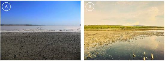
Figure 1.
Example of studied lakes of the Kerch Peninsula in summer with mud water: (A) Lake Tobechikskoye, (B) Lake Chokrakskoye.
Partially, the water bodies of the Kerch Peninsula are often used in fisheries []. Thus, Lake Aktashskoye, located in the north of the Kerch Peninsula, is used as a reservoir for breeding saltwater crustaceans Artemia salina, which are a natural source of astaxanthin, which is widely used in the dental and pharmaceutical industries [].
All this leads to the significant importance of these water bodies in the context of the economic development of the region, which makes it necessary to constantly monitor the water resources of these objects. However, since regular field monitoring is quite financially and resource-intensive, it becomes necessary to find a way for automated remote monitoring of water bodies using remote sensing data, which was the main goal of this work.
In previous studies, a method for extracting the water surface areas of the lakes of the Kerch Peninsula using QGIS and Python was tested []. The methodology was based on the use of the index, which helped to separate water bodies from land. As remote sensing data, Sentinel-2 images for the 2018 were used. To separate water from land, bands B3 (560 μm) and B11 (842 μm) were used using the index. In addition, to analyze the obtained results, the authors used annual data on air temperature and precipitation levels, which were obtained from the National Center for Environmental Information (NCEI CDO) at Kerch station (WMO code-33983). The seven largest lakes located in the study area were selected for monitoring—Aktashskoe, Chokrakskoe, Marfovskoe, Tobechikskoe, Kachik, Uzunlarskoe and Koyashskoe. The results of this study showed a fairly good accuracy, which made it possible to identify seasonal fluctuations in the water level of lakes. These fluctuations were caused mainly by dry weather and a prolonged lack of atmospheric precipitation, which, along with the absence of permanent sources of incoming water, leads to significant fluctuations in the water surface areas up to complete drying.
The problem of extracting water surface areas of water bodies is not new, especially in this region. Often, most studies are based on the use of various variations of water indices, the main direction of which is the determination of the water surface from land using the spectral channels of the green and middle-infrared parts of the spectrum. The main water indices, used in most of the studies are (McFeeters, []), (Xu, []), (Fisher et al. []) and (Feyisa et al. []) whose calculation formulas are as follows:
where , , , and are the reflectivity of remote sensing images in blue, green, near-infrared, shortwave-infrared and visible light bands, respectively.
A radically different approach was proposed by Li et al. []. The authors proposed a method based on the maximum entropy to extract the water surface. The implementation of this approach included several stages. At the beginning, the authors collected satellite data (Landsat 8 OLI and Landsat 5 TM). Then a “Water probability map” was calculated based on the MaxEnt Model which used Bands 1–7 from Landsat 5 and 8 and various spectral indices (, , , and
). At the next stage, the authors set the Objective Function MaxT, which can be expressed as []:
After that, it was meant to obtain the final result in the form of extracted data on the spatial distribution of water bodies in the study area.
Another way to extract water areas is using deep learning neural networks and SAR data. For example, in Bao et al. [], SAR images were used to extract water areas using feature analysis and dual-threshold graph cut model in case of flood monitoring. At the first stage, they applied a multiscale extraction using Gabor filter to reduce noise, and at the second stage, they used the Otsu algorithm and voting strategy to segment homogenous regions for Gaussian mixture model. As the result, the overall accuracy they reached was equal 99%.
The computer vision approach is another way that has great performance in cases using high resolution remote sensing data, obtained from free sources. In An and Rui [] lightweight U-Net architecture to extract water areas using Gaofen-2 satellite data. The main disadvantage of this approach is the limitation on the number of used bands. In most cases, to extract water areas using the computer vision approach, researchers are limited to using only three bands, which is good for territories and water areas with clean water and lack of mud.
Thus, the approach proposed in this study should solve disadvantages of other methods to increase the variability of the remote sensing data used and the specific environment where studied water bodies are situated.
2. Materials and Methods
2.1. Field Data Collection
Field data collection was caried out on Kerch Peninsula during quarterly expeditions organized by the Southern Federal University and Kerch State Maritime Technological University from 2017 to 2020 for monitoring of water areas of Kerch lakes (Figure 2).
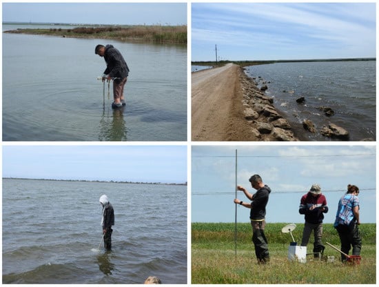
Figure 2.
Data collection during field expeditions for monitoring of the Kerch Peninsula lakes.
Besides water quality parameters, locations of the lakes water boundaries were collected using GPS navigator Garmin eTrex 10. All the collected data were processed in QGIS 3.22 to form a training dataset (Figure 3).
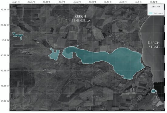
Figure 3.
Location of the area, which was used as a training dataset.
2.2. Remote Sensing Data
In this study, remote sensing data obtained using the Sentinel-2 satellite in the period from 2017 to 2022 during the days of field expeditions to map water bodies of the Kerch Peninsula were used.
As a training dataset, we used data on the spatial arrangement of the water surface on the Kerch Peninsula obtained during expeditionary studies conducted from 2017 to the present. To form this set, we used a test site located near Lake Tobechikskoye, where there are five water bodies (Figure 3).
The collected data were converted into a binary format, in which pixels characterizing water objects were marked as 1, and pixels containing land as 0. A ready-made data set necessary for training and testing a neural network was formed, representing this set of raster data as a two-dimensional array containing, in addition to the coordinates of latitude and longitude, the location of each pixel in space and an identifier for the presence of water, (Figure 4).
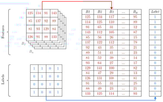
Figure 4.
Schematic representation of raster data in the array form. Red color represents features—reflectance data for each of the spectral bands of the Sentinel-2 satellite. Blue color represents binary values of presence (1) or absence (0) of water in each of the pixel. —raster band of the Sentinel-2 scene data. Numbers in tables represents different pixel values in bands of the Sentinel-2 data [].
General scheme of the presented methodology is presented in Figure 5.
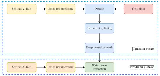
Figure 5.
General scheme of proposed methodology for water extraction using deep neural network and Sentinel-2 data.
2.3. Deep Neural Network Architecture
In this study, the Keras framework, written in Python to build the architecture of a deep neural network, was used. The architecture shown in Figure 6 consists of fully connected flatten (FL1) and four dense (DL1, DL2, DL3 and DL4) layers. The FL1 layer was used to “smooth” the input data, i.e., “straightening” 2- or more-dimensional matrices into one-dimensional vectors, transforming in this case a matrix of dimensions (1, 1, 12) into a one-dimensional vector with 6000 elements. The dense layers used in this architecture are simple fully connected layers, in which each neuron of the previous layer is connected to each neuron of the current layer. As activation functions in layers DL1, DL2 and DL3, the ReLU activation function was used, while on the last one-Softmax.
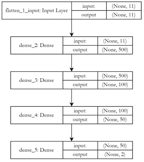
Figure 6.
Architecture of the model, used to extract water areas from remote sensing data.
The ReLU activation function [] returns 0 if the result takes a negative argument, while if it is positive, it returns the number itself, i.e.,
The use of this activation function allows to reduce computational costs due to the absence of complex mathematical operations, which will lead to a decrease in the training time of the model [].
On the DL4 output layer, the Softmax activation function [,] was used, which is often applied to the output layer when solving a classification problem. Its application leads to the fact that the sum of all output neurons is equal to 1, and the value of the interval {0,1} corresponding to each output is equated to the probabilities []. Mathematically, it can be represented as follows:
where: –elements of the input vector; –standard exponential function, which is applied to each element of ; –number of classes in the multiclass classifier (in case of binary classification = 2).
2.4. Accuracy Assessment
During the models training, the “sparse categorical crossentropy” as an accuracy metric [,] was used. It means that the probability of each predicted class is compared with the actual class output of 0 or 1, and a score/loss is calculated to penalize the probability based on how far it is from the actual expected value. The penalty is logarithmic in nature, giving a high score for large differences close to 1 and a low score for small differences approaching 0.
Cross-entropy loss is used when adjusting model weights during training. The goal is to minimize losses, i.e., the lower the loss, the better the model. The ideal model has a cross-entropy loss of 0.
For two classes, mathematically, it can be expressed as follows:
where –truth label taking a value or , and –Softmax probability for the -th class.
2.5. Validation of the Model Using Random Sample Points Dataset
As an alternative way to assess the accuracy of the model, 100 random points in the study area were selected, which were examined for the presence or absence of water in these places []. The scheme of randomly generated points is shown in Figure 7.
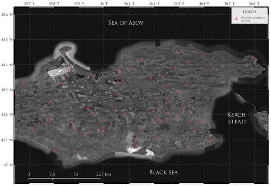
Figure 7.
Scheme of randomly generated points for validation of the model.
This procedure was chosen as an additional check after the synthetic testing of the model during its training.
The calculation of accuracy was carried out based on the confusion matrix (Table 1).

Table 1.
Confusion matrix for water extraction validation using random sampling points.
True positive (TP) is the number of times the water points are correctly classified by the model as the presence of waterTrue negative (TN)—the number of times the model correctly classified points without water as non-water points. False positive (FP) is the number of times it classified points with no water as having it. False negative (FN) is the number of times water points were classified as non-water.
Based on the obtained results, the accuracy metrics “Accuracy”, “Precision” and “Recall” were calculated:
These accuracy metrics will, in our opinion, make it possible to more adequately assess the performance of the model.
3. Results and Discussion
3.1. Training Configuration
An ASUS laptop with CPU of Intel i7-11370H (4 cores, 3.30 GHz), memory of 16 GB DDR4 and graphic card of NVIDIA GeForce RTX 3050 (4 GB) has been used for calculation. The data set was divided in the following proportion: 70% for training data, 10% for validation data and 20% for test data.
3.2. Deep Neural Network Performance
The total training time for the model was 21 min. 53.2 s. As can be seen from the Figure 5, the accuracy of the model reached values > 0.95 on 30 epoch, and by 40 epoch it reached ≈ 0.98 on training dataset.
The accuracy of the model on the validation dataset is slightly different. Thus, the model reached an accuracy level of >0.95 at the 26th iteration, and by the 40th iteration, the same accuracy was achieved as on the training data set ≈ 0.98. Cross-entropy loss, presented on figure for train and validation data, is similar. A level of loss < 0.1 was reached on the 25th epoch of both datasets (Figure 8).
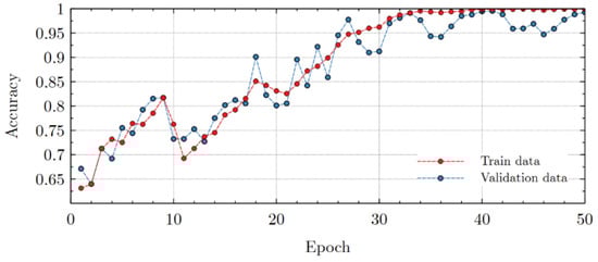
Figure 8.
Accuracy of the model, received after the models training stage.
According to the confusion matrix, presented in Figure 6, models prediction capabilities also showed a fairly high accuracy level. From the 100 test points, 96 of them were correctly classified, which, respectively, amounted to 96% of the accuracy of the model (Figure 9).
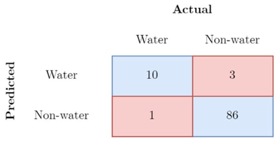
Figure 9.
Confusion matrix for water extraction validation using random sampling points.
The accuracy metrics by which the validation was made are presented in Table 2.
Table 2.
Accuracy metrics for water extraction validation using random sampling points.
As can be seen from Table 2, the selected metrics show lower performance. Thus, the lowest value in the predictive accuracy is at “precision” metric (0.76), while the highest is 0.96. Such a significant difference in accuracy estimated by various metrics describing models performance is largely due to the class imbalance problem, since when forming a set of point data for testing, the proportions of the classes were divided in the ratio of 1:9. This is largely due to the natural features of the study area, for which the presence of water resources on its surface is largely limited, and their ratio to the total area of the Kerch Peninsula, even in heavy rainfall seasons, is significantly small. Nevertheless, the presented results describing the accuracy of the model allow to conclude that high levels of accuracy have been achieved, which leads to its high predictive ability.
As a result, a map of the distribution of water bodies in the territory of the Kerch Peninsula for the summer of 2022 was obtained (Figure 10). Since the summer period in the study area is often characterized by dry weather and the absence of high precipitation levels, the areas of the peninsula occupied by water bodies are significantly small.
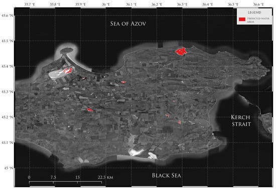
Figure 10.
Results of water extraction model on the Kerch Peninsula in summer 2022.
Comparison with previous results was carried out in a testing area near Lake Tobechikskoye. The results presented in Figure 11 show a great difference between results obtained during previous research, using for calculations, and the current approach, using a deep neural network. The main difference between these two calculations can be seen in areas with lakes that have a muddy environment. Due to the summer conditions, the areas of water bodies significantly decreased, which can be seen in results obtained using deep neural network []. Compared with the current approach, the methodology presented in previous research, based on calculations, showed less accurate results.
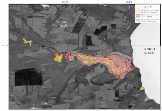
Figure 11.
Results of water extraction model different spectrum on the Kerch Peninsula in summer 2022.
Annual comparison of water area in Lake Tobechikskoye also showed better performance of the current deep neural network approach compared with calculations using . One of the main features of the water area of Lake Tobechikskoye is a great dependence on precipitation amount. Figure 12 shows the high increase in water area in spring and autumn, seasons with high level of precipitation, while in summer and winter, the water area slightly decreased, due to evaporation and water freezing. Compared with field investigations in 2018, deep neural network approach showed more accurate results.
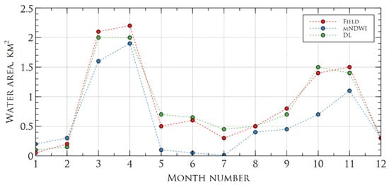
Figure 12.
Comparison of water area change in Lake Tobechikskoye in 2018, calculated using field investigations (red color), mNDWI index (blue color) and deep neural network (green color).
Particular attention should be paid to the peculiarities of the water bodies of the Kerch Peninsula. Most of these lakes have mud water, which poses difficulties in determining the areas of the water surface due to changes in the spectral signatures of directly fresh water and water with mud impurities. As a result of this phenomenon, erroneous definitions of the water surface as land can occur, which lead to distortions in the final results.
Despite this, taking into account the above facts, the model obtained in this study shows quite good results in the identification of water bodies using remote sensing data, which will make it possible to fully use this technology in the future both in hydrological studies and in the design and forecasting of fisheries activities.
In the future, we hope to combine data from Sentinel-2 satellite with SAR data and modify the architecture of the neural network to increase accuracy and overall performance of the model.
4. Conclusions
In this study, possibilities of water extraction using remote sensing data and a deep neural network were analyzed. Accordingly, we proposed a deep neural network, containing four layers for water body extraction, based on remote sensing data from the Sentinel-2 satellite. The results achieved allow to conclude that the trained model shows an acceptable level of accuracy, with a total error of about 4–5%. Compared with previous results, the proposed deep neural network also showed good performance. Moreover, it was shown that for long-term monitoring of the Kerch Peninsula’s lakes areas, both for fisheries and hydrological purposes, it is acceptable to use Sentinel-2 data with a deep neural network constructed using TensorFlow and the Keras pipeline.
Author Contributions
Conceptualization, D.K. and S.C.; methodology, L.B.; software, S.C.; validation, A.Z., L.B. and D.K.; formal analysis, S.C.; investigation, A.Z.; resources, D.K.; data curation, S.C.; writing—original draft preparation, D.K.; visualization, D.K.; supervision, A.Z.; project administration, S.C.; funding acquisition, A.Z. All authors have read and agreed to the published version of the manuscript.
Funding
The research is partially funded by the Ministry of Science and Higher Education of the Russian Federation as part of the World-class Research Center program: Advanced Digital Technologies (contract No. 075-15-2022-312 dated 20 April 2022).
Institutional Review Board Statement
Not applicable.
Informed Consent Statement
Not applicable.
Data Availability Statement
Not applicable.
Conflicts of Interest
The authors declare no conflict of interest.
References
- Sokol, E.V.; Kokh, S.N.; Kozmenko, O.A.; Lavrushin, V.Y.; Belogub, E.V.; Khvorov, P.V.; Kikvadze, O.E. Boron in an onshore mud volcanic environment: Case study from the Kerch Peninsula, the Caucasus continental collision zone. Chem. Geol. 2019, 525, 58–81. [Google Scholar] [CrossRef]
- Kharytonov, M.M.; Mitsik, O.; Stankevich, S.; Titarenko, O. Geomining Site Ecological Assessment and Reclamation Along Coastal Line of the Kerch Peninsula. In Black Sea Energy Resource Development and Hydrogen Energy Problems; Veziroğlu, A., Tsitskishvili, M., Eds.; Springer: Dordrecht, The Netherlands, 2013; pp. 325–336. [Google Scholar]
- Kayukova, E. Resources of Curative Mud of the Crimea Peninsula. In Thermal and Mineral Waters: Origin, Properties and Applications; Balderer, W., Porowski, A., Idris, H., LaMoreaux, J.W., Eds.; Environmental Earth Sciences; Springer: Berlin/Heidelberg, Germany, 2014; pp. 61–72. ISBN 978-3-642-28824-1. [Google Scholar]
- Zakharov, V.S.; Simonov, D.A.; Bryantseva, G.V.; Kosevich, N.I. Self-Similarity Properties of the Kerch Peninsula Stream Network and Their Comparison with the Results of Structural and Geomorphological Analysis. Izv. Atmos. Ocean. Phys. 2019, 55, 721–730. [Google Scholar] [CrossRef]
- Borovskaya, R.; Krivoguz, D.; Chernyi, S.; Kozhurin, E.; Zinchenko, E. Surface Water Salinity Evaluation and Identification for Using Remote Sensing Data and Machine Learning Approach. J. Mar. Sci. Eng. 2022, 10, 257. [Google Scholar] [CrossRef]
- Krivoguz, D.; Bespalova, L. Landslide susceptibility analysis for the Kerch Peninsula using weights of evidence approach and GIS. Russ. J. Earth Sci. 2020, 20, ES1003. [Google Scholar] [CrossRef]
- Krivoguz, D.; Bespalova, L. Analysis of Kerch Peninsula’s climatic parameters in scope of landslide susceptibility. Bull. KSMTU 2018, 1, 5–11. [Google Scholar]
- Kotov, S.; Kotova, I.; Kayukova, E. Geological controls and the impact of human society on the composition of peloids of present-day salt lakes (coastal zones of the Black, Azov, and Dead Seas). J Coast Conserv 2019, 23, 843–855. [Google Scholar] [CrossRef]
- Ovsyuchenko, A.N.; Vakarchuk, R.N.; Korzhenkov, A.M.; Larkov, A.S.; Sysolin, A.I.; Rogozhin, E.A.; Marakhanov, A.V. Active Faults in the Kerch Peninsula: New Results. Dokl. Earth Sc. 2019, 488, 1152–1156. [Google Scholar] [CrossRef]
- Kokh, S.N.; Shnyukov, Y.F.; Sokol, E.V.; Novikova, S.A.; Kozmenko, O.A.; Semenova, D.V.; Rybak, E.N. Heavy carbon travertine related to methane generation: A case study of the Big Tarkhan cold spring, Kerch Peninsula, Crimea. Sediment. Geol. 2015, 325, 26–40. [Google Scholar] [CrossRef]
- Trikhunkov, Y.I.; Bachmanov, D.M.; Gaidalenok, O.V.; Marinin, A.V.; Sokolov, S.A. Recent Mountain Building at the Junction Zone of the Northwestern Caucasus and Intermediate Kerch–Taman Region, Russia. Geotectonics 2019, 53, 517–532. [Google Scholar] [CrossRef]
- Borovskaya, R.V.; Zhugaylo, S.S.; Pugach, M.N.; Adzhiumerov, E.N.; Krivoguz, D.O. Current state of the habitat of commercial invertebrates in the hypersaline lakes of Crimea. Aquat. Bioresour. Environ. 2020, 3, 35–49. [Google Scholar] [CrossRef]
- Sobolev, A.S.; Chernyi, S.G.; Krivoguz, D.O.; Nyrkov, A.P.; Zinchenko, E.G. Convolution Neural Network for Identification of Underwater Objects. In Proceedings of the IEEE—2022 Conference of Russian Young Researchers in Electrical and Electronic Engineering (ElConRus), St. Petersburg, Russia, 25–28 January 2022; pp. 455–458. [Google Scholar]
- Krivoguz, D.; Mal’ko, S.; Borovskaya, R.; Semenova, A. Automatic processing of Sentinel-2 image for Kerch peninsula lake areas extraction using QGIS and Python. In Proceedings of the E3S Web of Conferences 2020, Blagoveshchensk, Russia, 23–24 September 2020; Volume 203, p. 3011. [Google Scholar]
- McFeeters, S.K. The use of the Normalized Difference Water Index (NDWI) in the delineation of open water features. Int. J. Remote Sens. 1996, 17, 1425–1432. [Google Scholar] [CrossRef]
- Xu, H. Modification of normalised difference water index (NDWI) to enhance open water features in remotely sensed imagery. Int. J. Remote Sens. 2006, 27, 3025–3033. [Google Scholar] [CrossRef]
- Fisher, A.; Flood, N.; Danaher, T. Comparing Landsat water index methods for automated water classification in eastern Australia. Remote Sens. Environ. 2016, 175, 167–182. [Google Scholar] [CrossRef]
- Feyisa, G.L.; Meilby, H.; Fensholt, R.; Proud, S.R. Automated Water Extraction Index: A new technique for surface water mapping using Landsat imagery. Remote Sens. Environ. 2014, 140, 23–35. [Google Scholar] [CrossRef]
- Li, W.; Zhang, W.; Li, Z.; Wang, Y.; Chen, H.; Gao, H.; Zhou, Z.; Hao, J.; Li, C.; Wu, X. A new method for surface water extraction using multi-temporal Landsat 8 images based on maximum entropy model. Eur. J. Remote Sens. 2022, 55, 303–312. [Google Scholar] [CrossRef]
- Bao, L.; Lv, X.; Yao, J. Water Extraction in SAR Images Using Features Analysis and Dual-Threshold Graph Cut Model. Remote Sens. 2021, 13, 3465. [Google Scholar] [CrossRef]
- An, S.; Rui, X. A High-Precision Water Body Extraction Method Based on Improved Lightweight U-Net. Remote Sens. 2022, 14, 4127. [Google Scholar] [CrossRef]
- Perikamana, K.K.; Balakrishnan, K.; Tripathy, P. A CNN based method for Sub-pixel Urban Land Cover Classification using Landsat-5 TM and Resourcesat-1 LISS-IV Imagery. arXiv 2021, arXiv:2112.08841. [Google Scholar] [CrossRef]
- Agarap, A.F. Deep Learning using Rectified Linear Units (ReLU). arXiv 2019, arXiv:1803.08375. [Google Scholar] [CrossRef]
- Chernyi, S.; Emelianov, V.; Zinchenko, E.; Zinchenko, A.; Tsvetkova, O.; Mishin, A. Application of Artificial Intelligence Technologies for Diagnostics of Production Structures. J. Mar. Sci. Eng. 2022, 10, 259. [Google Scholar] [CrossRef]
- Wang, M.; Lu, S.; Zhu, D.; Lin, J.; Wang, Z. A High-Speed and Low-Complexity Architecture for Softmax Function in Deep Learning. In Proceedings of the 2018 IEEE Asia Pacific Conference on Circuits and Systems (APCCAS), Chengdu, China, 26–30 October 2018; pp. 223–226. [Google Scholar]
- Gao, B.; Pavel, L. On the Properties of the Softmax Function with Application in Game Theory and Reinforcement Learning. arXiv 2018, arXiv:1704.00805. [Google Scholar] [CrossRef]
- Zhilenkov, A.; Chernyi, S.; Emelianov, V. Application of Artificial Intelligence Technologies to Assess the Quality of Structures. Energies 2021, 14, 8040. [Google Scholar] [CrossRef]
- Covington, P.; Adams, J.; Sargin, E. Deep Neural Networks for YouTube Recommendations. In Proceedings of the 10th ACM Conference on Recommender Systems, Boston, MA, USA, 15–19 September 2016; Association for Computing Machinery: New York, NY, USA, 2016; pp. 191–198. [Google Scholar]
- Kakarla, J.; Isunuri, B.V.; Doppalapudi, K.S.; Bylapudi, K.S.R. Three-class classification of brain magnetic resonance images using average-pooling convolutional neural network. Int. J. Imaging Syst. Technol. 2021, 31, 1731–1740. [Google Scholar] [CrossRef]
- Skripka, G.; Ivlieva, O.; Bespalova, L.; Filatov, A.; Saprygin, V. Monitoring of dangerous shore processes of Tsimlyansk Reservoir using GIS-technologies. ICIGIS 2020, 26, 253–263. [Google Scholar] [CrossRef]
Publisher’s Note: MDPI stays neutral with regard to jurisdictional claims in published maps and institutional affiliations. |
© 2022 by the authors. Licensee MDPI, Basel, Switzerland. This article is an open access article distributed under the terms and conditions of the Creative Commons Attribution (CC BY) license (https://creativecommons.org/licenses/by/4.0/).