Classifying Headland-Bay Beaches and Dynamic Coastal Stabilization

 ,
,  and
and
Abstract
:1. Introduction
2. Materials and Methods
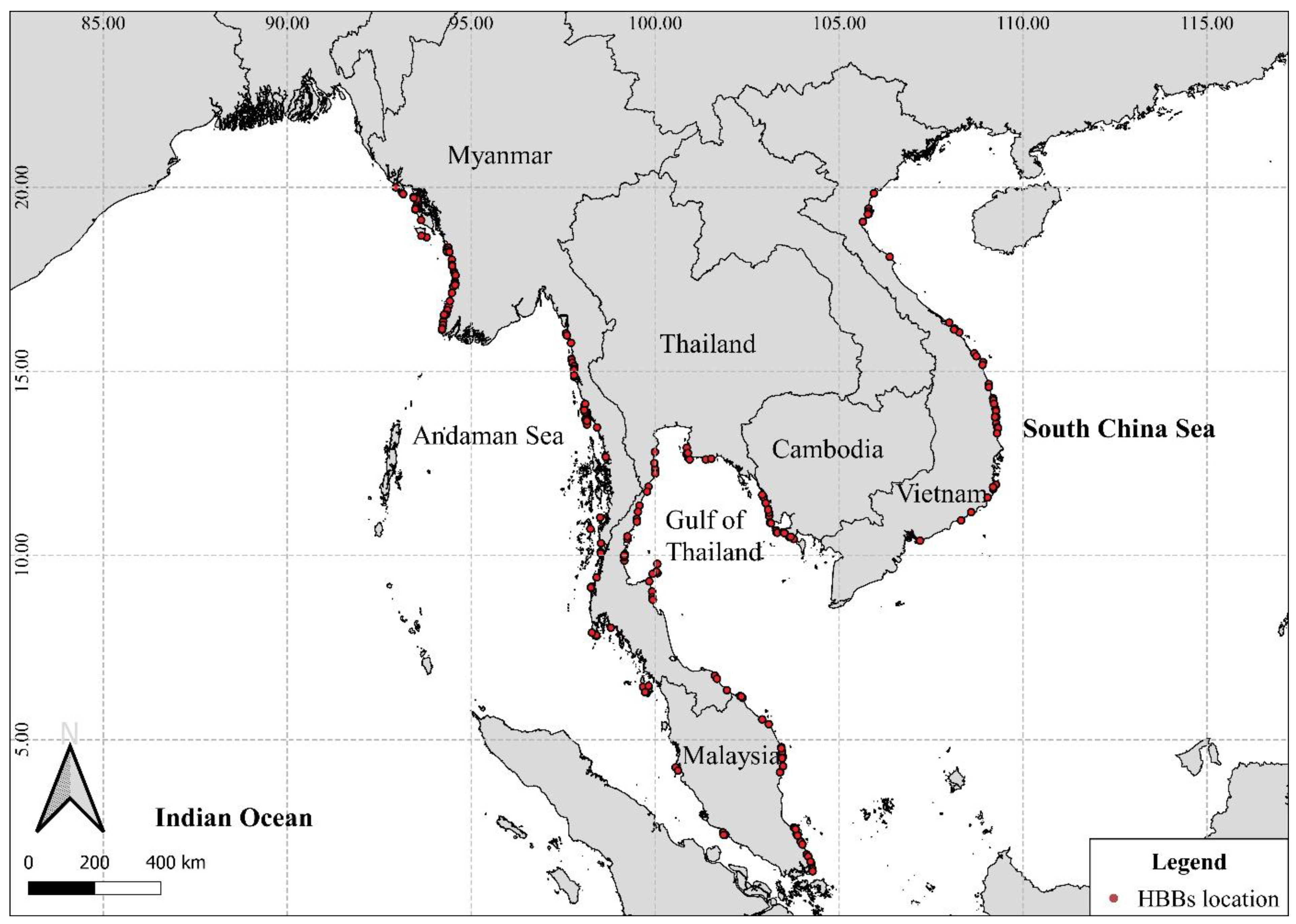
2.1. Study Area
2.2. General Methodological Remarks
2.2.1. Types of Headland-Bay Beaches
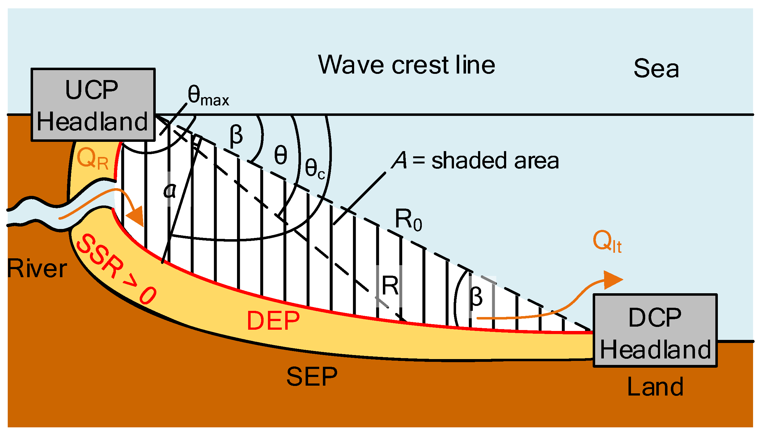
2.2.2. Bay Planform Equations
2.2.3. Bay Characteristic Equations
2.3. Materials
2.3.1. Satellite Images
2.3.2. Field Sediment Supply Ratio
2.4. Approach
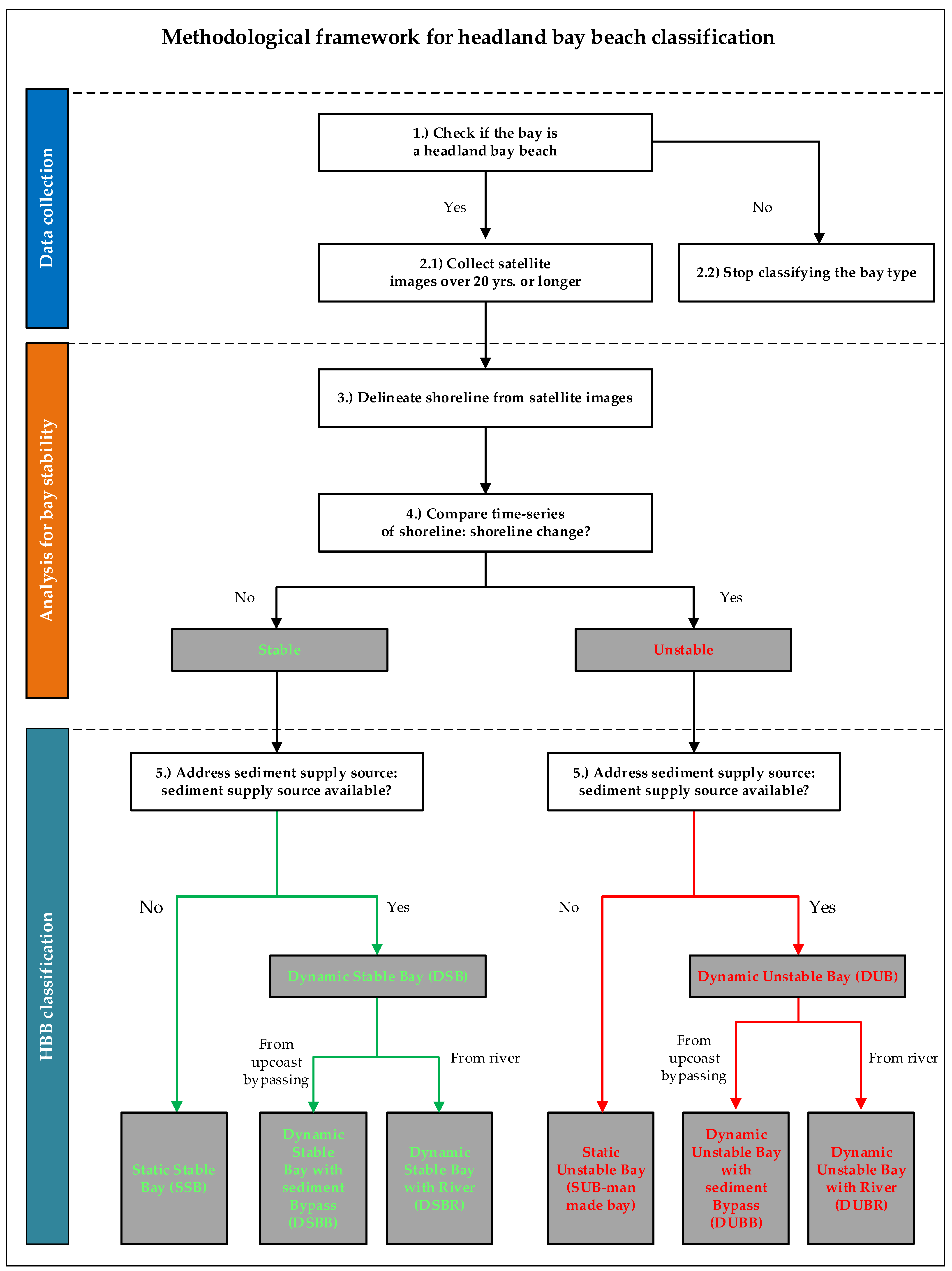
2.4.1. Development of Headland-Bay Beach Classification Framework
2.4.2. Verification of Bay Planform Equation
2.4.3. Verification of Bay Characteristic Equations
3. Results
3.1. Types of Headland-Bay Beaches in Southeast Asia
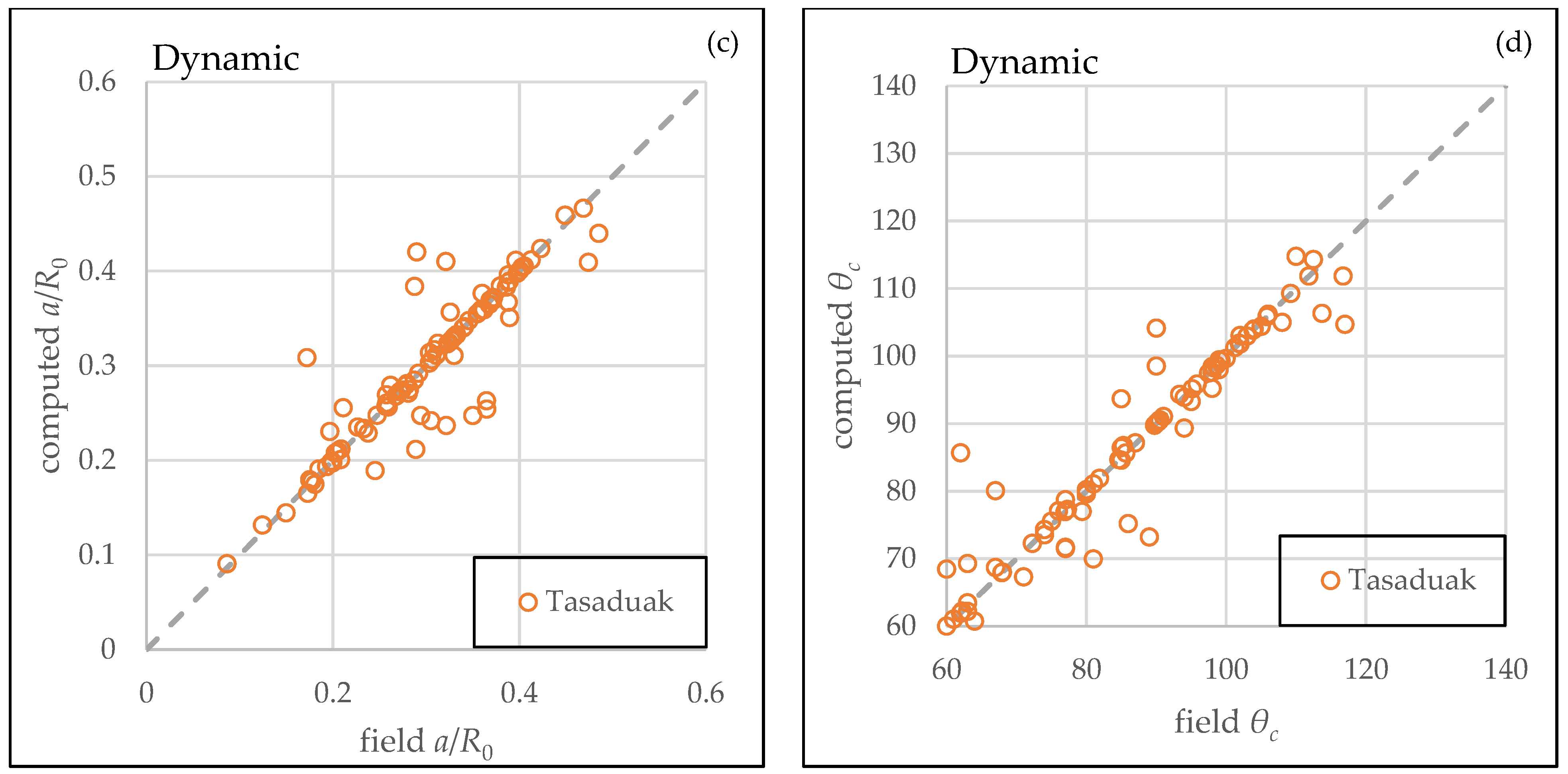
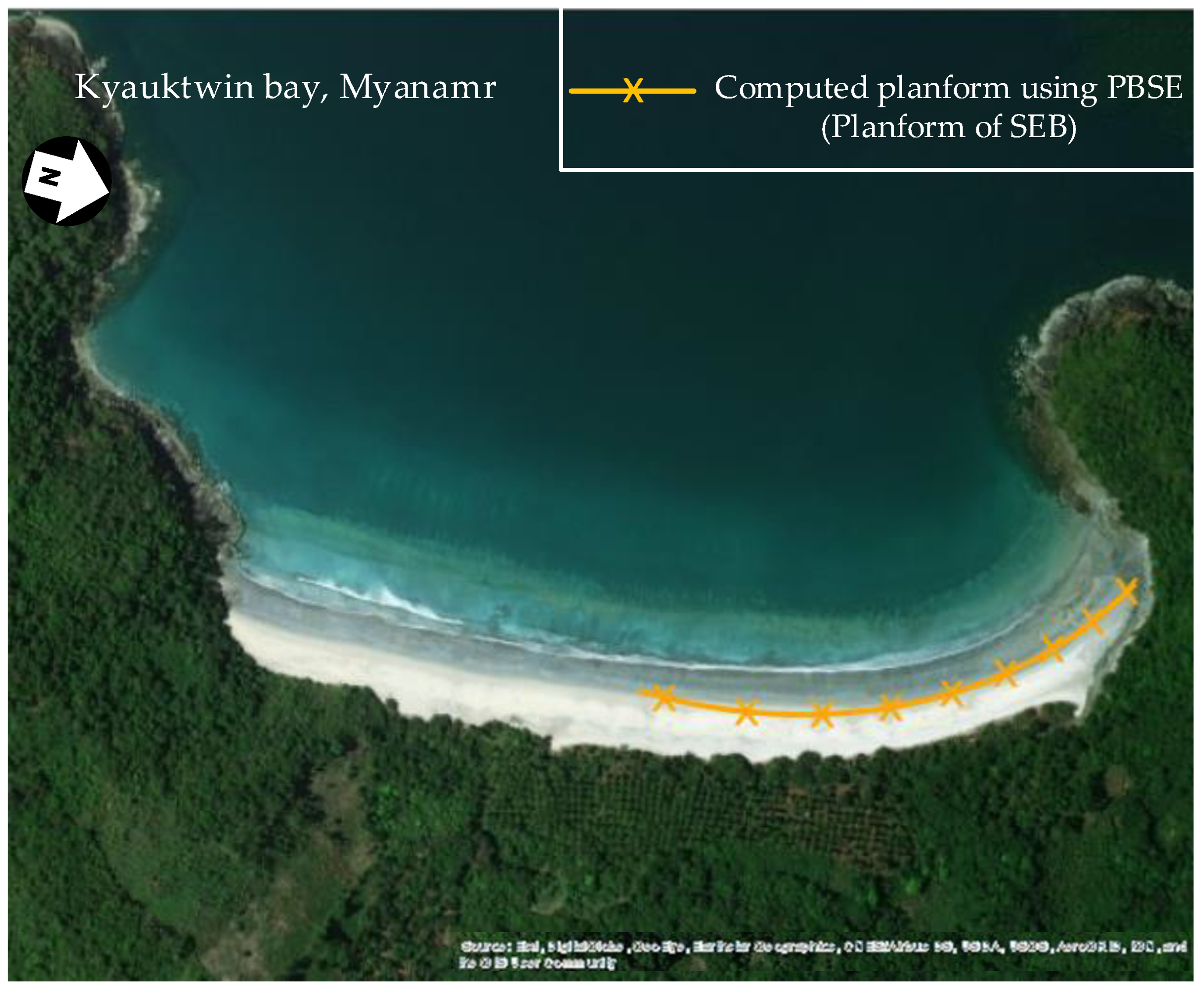
3.2. Verification of Dynamic Parabolic Bay Shape Equation (DPBSE)
3.3. Stable Bays in Southeast Asia
3.4. Performance of Bay Characteristic Equations
4. Discussion
4.1. Headland-Bay Beach Classification Framework
4.2. Dynamic Bay Planform Equation
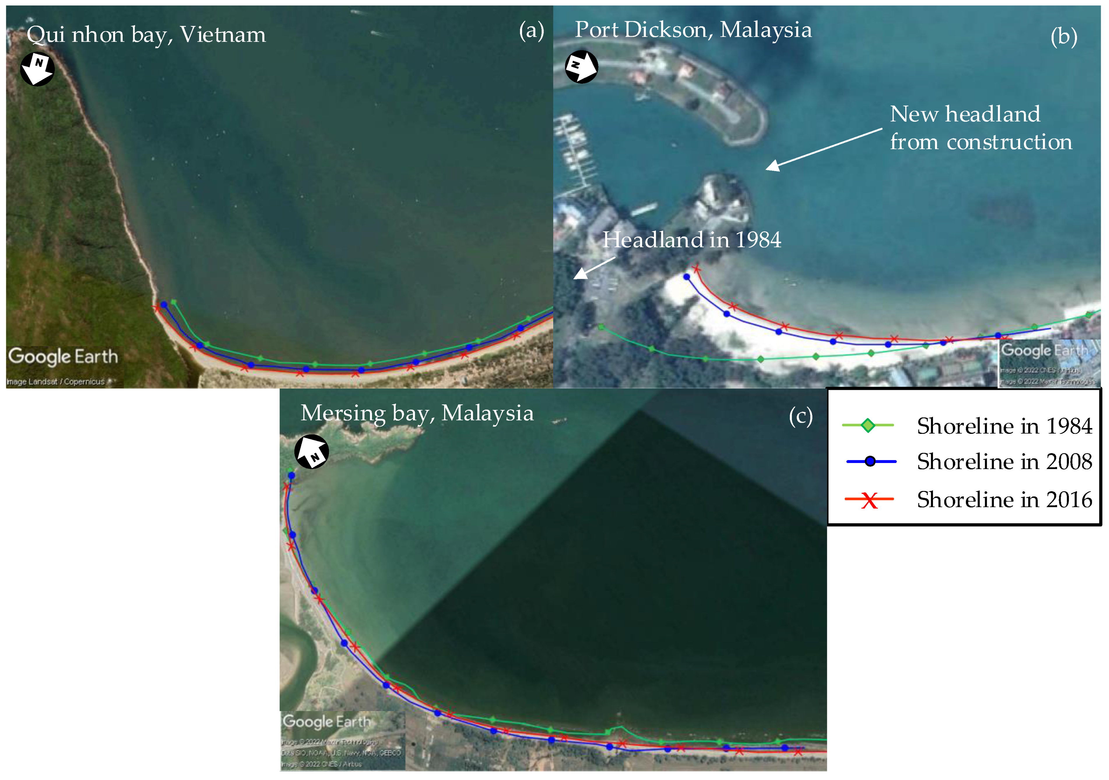
4.3. Characteristics of Stable Bays in Southeast Asia
4.4. Bay Characteristic Equations
4.5. Sensitivity Analysis
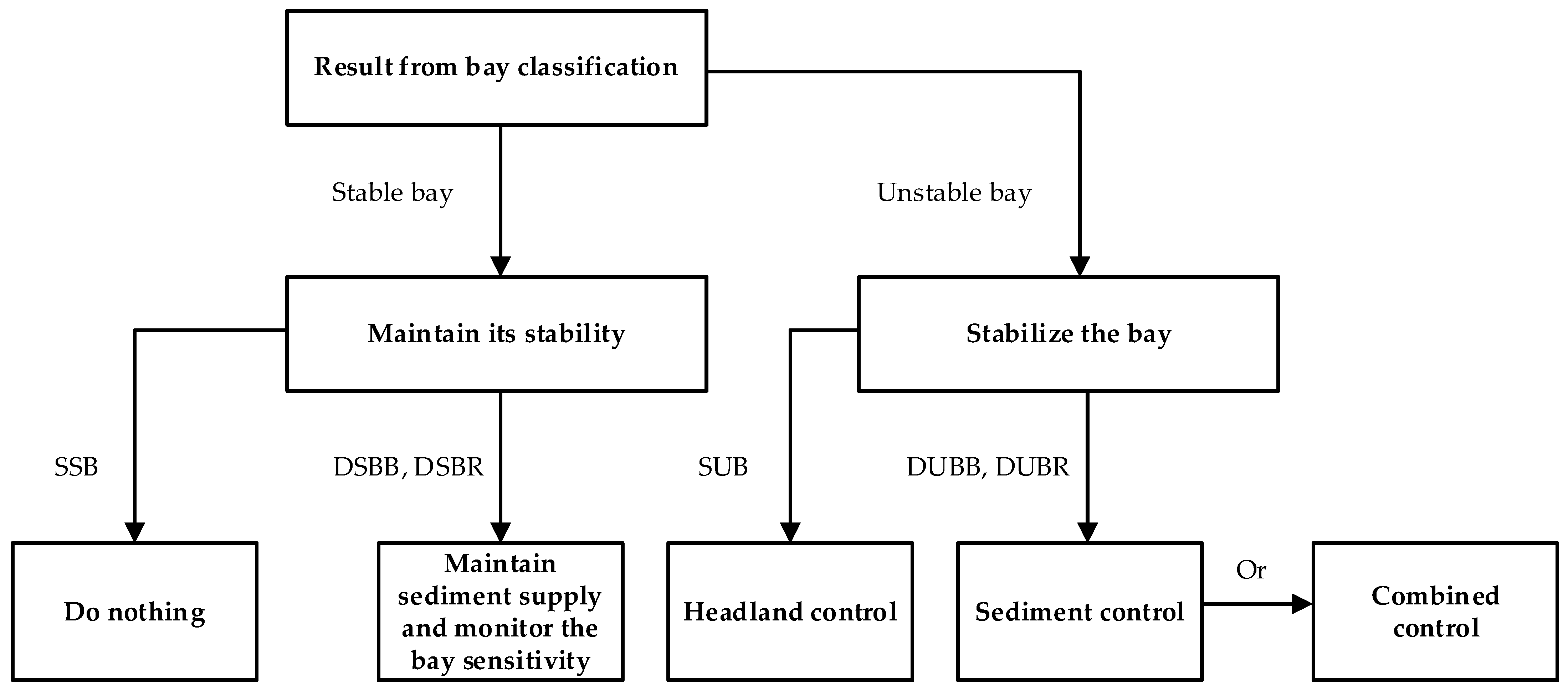
4.6. Coastal Stabilization for Dynamic Bays
5. Conclusions
Author Contributions
Funding
Institutional Review Board Statement
Informed Consent Statement
Conflicts of Interest
Appendix A

| Country | Type | Number of Bays | Percentage | ||||
|---|---|---|---|---|---|---|---|
| Stable | Unstable | Total | Stable (%) | Unstable (%) | |||
| Cambodia | Static | 1 | 5 | 6 | 16.67 | 83.33 | |
| Dynamic | Bypass | 6 | 0 | 6 | 100.00 | 0.00 | |
| River | 5 | 2 | 7 | 71.43 | 28.57 | ||
| All | 11 | 2 | 13 | 84.62 | 15.38 | ||
| Total | 12 | 7 | 19 | 63.16 | 36.84 | ||
| Malaysia | Static | 2 | 6 | 8 | 25.00 | 75.00 | |
| Dynamic | Bypass | 9 | 8 | 17 | 52.94 | 47.06 | |
| River | 7 | 8 | 15 | 46.67 | 53.33 | ||
| All | 16 | 16 | 32 | 50.00 | 50.00 | ||
| Total | 18 | 22 | 40 | 45.00 | 55.00 | ||
| Myanmar | Static | 20 | 4 | 24 | 83.33 | 16.67 | |
| Dynamic | Bypass | 17 | 1 | 18 | 94.44 | 5.56 | |
| River | 30 | 2 | 32 | 93.75 | 6.25 | ||
| All | 47 | 3 | 50 | 94.00 | 6.00 | ||
| Total | 67 | 7 | 74 | 90.54 | 9.46 | ||
| Thailand | Static | 12 | 7 | 19 | 63.16 | 36.84 | |
| Dynamic | Bypass | 6 | 12 | 18 | 33.33 | 66.67 | |
| River | 3 | 2 | 5 | 60.00 | 40.00 | ||
| All | 9 | 14 | 23 | 39.13 | 60.87 | ||
| Total | 21 | 21 | 42 | 50.00 | 50.00 | ||
| Vietnam | Static | 14 | 6 | 20 | 70.00 | 30.00 | |
| Dynamic | Bypass | 8 | 1 | 9 | 88.89 | 11.11 | |
| River | 6 | 2 | 8 | 75.00 | 25.00 | ||
| All | 14 | 3 | 17 | 82.35 | 17.65 | ||
| Total | 28 | 9 | 37 | 75.68 | 24.32 | ||
| All | Static | 49 | 28 | 77 | 63.64 | 36.36 | |
| Dynamic | Bypass | 46 | 22 | 68 | 67.65 | 32.35 | |
| River | 51 | 16 | 67 | 76.12 | 23.88 | ||
| All | 97 | 38 | 135 | 71.85 | 28.15 | ||
| Total | 146 | 66 | 212 | 68.87 | 31.13 | ||
| Country | Type | R0 (km) | β (deg) | θmax (deg) | SSR | a (km) | a/R0 | θc (deg) | A (km2) | |
|---|---|---|---|---|---|---|---|---|---|---|
| Cambodia | SSB | range | 1.59 | 37.66 | 125.00 | - | 0.64 | 0.40 | 102.00 | 0.86 |
| mean | 1.59 | 37.66 | 125.00 | - | 0.64 | 0.40 | 102.00 | 0.86 | ||
| SD | - | - | - | - | - | - | - | - | ||
| DSBB | range | 0.79–9.97 | 24.35–46.00 | 75.00–133.00 | 0.03–0.88 | 0.16–2.56 | 0.20–0.37 | 62.00–98.00 | 0.09–17.36 | |
| mean | 2.69 | 29.61 | 99.33 | 0.24 | 0.71 | 0.27 | 77.83 | 3.17 | ||
| SD | 3.59 | 8.20 | 22.29 | 0.33 | 0.91 | 0.06 | 12.84 | 6.95 | ||
| DSBR | range | 0.96–4.28 | 37.2–56.57 | 112.50–172.00 | 0.01–0.36 | 0.45–1.81 | 0.29–0.47 | 81.00–110.00 | 0.35–6.83 | |
| mean | 2.09 | 46.20 | 139.60 | 0.15 | 0.81 | 0.38 | 99.40 | 1.92 | ||
| SD | 1.30 | 7.79 | 28.34 | 0.17 | 0.57 | 0.07 | 11.22 | 2.76 | ||
| Malaysia | SSB | range | 0.37–0.45 | 42.65–45.94 | 129.50–132.00 | - | 0.16–0.20 | 0.43–0.44 | 106.67–109.94 | 0.05–0.08 |
| mean | 0.41 | 44.30 | 130.75 | - | 0.18 | 0.44 | 108.31 | 0.07 | ||
| SD | 0.06 | 2.33 | 1.77 | - | 0.03 | 0.01 | 2.31 | 0.02 | ||
| DSBB | range | 0.54–1.39 | 23.15–50.26 | 80.00–158.50 | 0.07–0.81 | 0.12–0.39 | 0.18–0.4 | 53.00–106.00 | 0.05–0.32 | |
| mean | 0.81 | 33.65 | 128.06 | 0.28 | 0.22 | 0.28 | 76.9 | 0.14 | ||
| SD | 0.26 | 11.19 | 28.31 | 0.26 | 0.09 | 0.09 | 20.42 | 0.10 | ||
| DSBR | range | 0.32–6.13 | 28.61–51.23 | 60.00–171.50 | 0.02–0.91 | 0.10–2.26 | 0.23–0.41 | 60.00–103.84 | 0.02–10.98 | |
| mean | 3.03 | 40.00 | 128.07 | 0.22 | 1.04 | 0.34 | 90.33 | 3.64 | ||
| SD | 2.12 | 8.26 | 36.26 | 0.31 | 0.81 | 0.07 | 15.9 | 3.98 | ||
| Myanmar | SSB | range | 0.61–3.84 | 13.00–56.18 | 93.00–172.00 | - | 0.23–1.20 | 0.24–0.48 | 82.00–119.43 | 0.12–5.04 |
| mean | 1.47 | 36.50 | 121.45 | - | 0.51 | 0.36 | 99.08 | 0.90 | ||
| SD | 0.84 | 10.53 | 23.51 | - | 0.26 | 0.07 | 10.41 | 1.22 | ||
| DSBB | range | 0.26–6.5 | 12.08–48.52 | 74.50–165.00 | 0.02–0.50 | 0.08–1.97 | 0.19–0.47 | 43–117 | 0.02–3.98 | |
| mean | 1.72 | 31.81 | 116.85 | 0.17 | 0.51 | 0.30 | 81.85 | 0.82 | ||
| SD | 1.71 | 10.04 | 22.14 | 0.13 | 0.50 | 0.07 | 19.23 | 1.19 | ||
| DSBR | range | 0.63–9.80 | 7.80–65.08 | 78.00–148.00 | 0.02–0.95 | 0.19–2.04 | 0.09–0.41 | 53.57–111.83 | 0.07–10.89 | |
| mean | 3.07 | 34.35 | 113.15 | 0.16 | 0.82 | 0.30 | 84.07 | 2.45 | ||
| SD | 2.20 | 13.69 | 17.57 | 0.19 | 0.51 | 0.09 | 17.22 | 2.84 | ||
| Thailand | SSB | range | 0.39–3.93 | 21–56.31 | 84.00–149.50 | - | 0.12–1.75 | 0.22–0.54 | 71.00–119.55 | 0.04–5.14 |
| mean | 1.55 | 35.52 | 111.67 | - | 0.56 | 0.35 | 90.95 | 1.16 | ||
| SD | 1.20 | 12.30 | 17.27 | - | 0.51 | 0.10 | 15.89 | 1.73 | ||
| DSBB | range | 0.60–4.99 | 32.59–50.80 | 110.00–151.50 | 0.07–0.35 | 0.21–1.73 | 0.27–0.45 | 77.12–112.48 | 0.12–6.26 | |
| mean | 2.13 | 42.00 | 122.50 | 0.20 | 0.77 | 0.34 | 93.12 | 1.76 | ||
| SD | 1.72 | 7.70 | 15.84 | 0.13 | 0.66 | 0.07 | 14.06 | 2.40 | ||
| DSBR | range | 0.46–2.34 | 16.83–36.53 | 90.00–137.00 | 0.05–1.19 | 0.15–0.28 | 0.12–0.33 | 85.31–137 | 0.05–0.48 | |
| mean | 1.15 | 29.05 | 113.17 | 0.45 | 0.21 | 0.25 | 104.02 | 0.21 | ||
| SD | 1.04 | 10.67 | 23.51 | 0.64 | 0.06 | 0.12 | 28.65 | 0.24 | ||
| Vietnam | SSB | range | 0.64–4.01 | 30.63–57.13 | 90.00–154.50 | - | 0.27–1.66 | 0.36–0.47 | 89.5–116.34 | 0.15–5.50 |
| mean | 1.69 | 45.7 | 118.00 | - | 0.71 | 0.43 | 105.59 | 1.39 | ||
| SD | 1.12 | 8.26 | 17.37 | - | 0.43 | 0.04 | 8 | 1.73 | ||
| DSBB | range | 9.97 | 25.79 | 76.00 | 0.07 | 2.57 | 0.26 | 76.00 | 17.75 | |
| mean | 9.97 | 25.79 | 76.00 | 0.07 | 2.57 | 0.26 | 76.00 | 17.75 | ||
| SD | - | - | - | - | - | - | - | - | ||
| DSBR | range | 1.02–9.06 | 14.45–51.67 | 67–154.5 | 0.03–0.37 | 0.26–2.3 | 0.15–0.49 | 49–116.75 | 0.27–12.74 | |
| mean | 4.69 | 32.77 | 116.19 | 0.12 | 1.3 | 0.29 | 80.05 | 5.38 | ||
| SD | 2.51 | 13.31 | 25.12 | 0.10 | 0.66 | 0.09 | 20.33 | 4.24 | ||
| All | SSB | range | 0.37–4.01 | 13.00–57.13 | 84.00–172.00 | - | 0.12–1.75 | 0.22–0.54 | 71.00–119.55 | 0.04–5.50 |
| mean | 1.51 | 39.23 | 118.52 | - | 0.57 | 0.38 | 99.38 | 1.07 | ||
| SD | 1.00 | 10.82 | 19.78 | - | 0.39 | 0.08 | 12.28 | 1.47 | ||
| DSBB | range | 0.26–9.97 | 12.08–50.80 | 74.50–165.00 | 0.02–0.88 | 0.08–2.57 | 0.18–0.47 | 43.00–117.00 | 0.02–17.75 | |
| mean | 1.93 | 33.31 | 116.56 | 0.21 | 0.57 | 0.30 | 81.67 | 1.60 | ||
| SD | 2.33 | 10.10 | 24.51 | 0.20 | 0.65 | 0.07 | 17.90 | 3.97 | ||
| DSBR | range | 0.32–9.8 | 7.80–65.08 | 60.00–172.00 | 0.01–1.19 | 0.10–2.30 | 0.09–0.49 | 49.00–137.00 | 0.02–12.74 | |
| mean | 3.25 | 35.42 | 117.91 | 0.18 | 0.92 | 0.31 | 86.28 | 3.09 | ||
| SD | 2.30 | 12.85 | 23.91 | 0.23 | 0.62 | 0.09 | 18.63 | 3.48 | ||
References
- Inman, D.L.; Nordstrom, C.E. On the tectonic and morphologic classification of coasts. J. Geol. 1971, 79, 1–21. [Google Scholar] [CrossRef]
- Short, A.D.; Masselink, G. Embayed and structurally controlled beaches. In Handbook of Beach and Shoreface Morphodynamics; Short, A.D., Ed.; Wiley: New York, NY, USA, 1999; Volume 1, pp. 230–249. [Google Scholar]
- Klein, A.H.; Filho, L.B.; Hsu, J.R.C. Stability of headland bay beaches in Santa Catarina: A case study. J. Coast. Res. 2003, 2003, 151–166. [Google Scholar]
- Kemp, J.; Vandeputte, B.; Eccleshall, T.; Simons, R.; Troch, P. A modified hyperbolic tangent equation to determine equilibrium shape of headland bay beaches. Coast. Eng. Proc. 2018, 1, 106. [Google Scholar] [CrossRef]
- Hsu, J.R.C.; Yu, M.J.; Lee, F.C.; Benedet, L. Static bay beach concept for scientists and engineers: A review. Coast. Eng. 2010, 57, 76–91. [Google Scholar] [CrossRef]
- Silvester, R.; Hsu, J.R.C. Coastal Stabilization: Innovative Concepts; Prentice-Hall: New Jersey, NJ, USA, 1993. [Google Scholar]
- Silvester, R.; Hsu, J.R.C. Coastal Stabilization; World Scientific: Singapore, 1997; Volume 14. [Google Scholar]
- Tasaduak, S. Dynamic Equilibrium of Crenulated Shaped Bays; Asian Institute of Techology: Pathum Thani, Thailand, 2014. [Google Scholar]
- Tasaduak, S.; Weesakul, S. Experimental study on dynamic equilibrium of headland-bay beaches. J. Coast. Conserv. 2016, 20, 165–174. [Google Scholar] [CrossRef]
- Tasaduak, S.; Weesakul, S.; Babel, M.S.; Clemente, R.S.; Phien-Wej, N. Equilibrium of crenulated bays in Thailand. Coast. Eng. J. 2014, 56, 1450019-1–1450019-19. [Google Scholar] [CrossRef]
- Gupta, A. Erosion and sediment yield in Southeast Asia: A regional perspective. In Proceedings of the Erosion and Sediment Yield: Global and Regional Perspectives, Exeter, UK, 15–19 July 1996; pp. 215–222. [Google Scholar]
- Luijendijk, A.; Hagenaars, G.; Ranasinghe, R.; Baart, F.; Donchyts, G.; Aarninkhof, S. The state of the world’s beaches. Sci. Rep. 2018, 8, 1–11. [Google Scholar] [CrossRef]
- Zhang, Y.; Hou, X. Characteristics of coastline changes on southeast Asia Islands from 2000 to 2015. Remote Sens. 2020, 12, 519. [Google Scholar] [CrossRef]
- Chuan, G.K. The climate of southeast Asia. In The Physical Geography of Southeast Asia; Gupta, A., Ed.; Oxford University Press: Oxford, UK, 2005; pp. 80–93. [Google Scholar]
- Wong, P. The coastal environment of Southeast Asia. In The Physical Geography of Southeast Asia; Gupta, A., Ed.; Oxford University Press: Oxford, UK, 2005. [Google Scholar]
- Quirapas, M.A.J.R.; Lin, H.; Abundo, M.L.S.; Brahim, S.; Santos, D. Ocean renewable energy in Southeast Asia: A review. Renew. Sust. Energy. Rev. 2015, 41, 799–817. [Google Scholar] [CrossRef]
- Short, A.D. Wave-dominated, tide-modified and tide-dominated continuum. In Sand Beach Morphodynamics; Elsevier: Amsterdam, The Netherlands, 2020; pp. 363–389. [Google Scholar]
- Hsu, J.R.C.; Evans, C. Parabolic bay shapes and applications. Inst. Civ. Eng. 1989, 87, 557–570. [Google Scholar] [CrossRef]
- Yasso, W.E. Plan geometry of headland-bay beaches. J. Geol. 1965, 73, 702–714. [Google Scholar] [CrossRef]
- Moreno, L.J.; Kraus, N.C. Equilibrium Shape of Headland-Bay Beaches for Engineering Design. Coastal Defense Program Madrid (Spain). 1999. Available online: https://apps.dtic.mil/sti/pdfs/ADA483142.pdf (accessed on 20 July 2021).
- González, M.; Medina, R. On the application of static equilibrium bay formulations to natural and man-made beaches. Coast. Eng. 2001, 43, 209–225. [Google Scholar] [CrossRef]
- Vichetpan, N. Equilibrium Shapes of Coastline in Plan; Asian Institute of Technology: Pathum Thani, Thailand, 1969. [Google Scholar]
- Ho, S.K. Crenulate Shaped Bays; Asian Institute of Technology: Pathum Thani, Thailand, 1971. [Google Scholar]
- Tan, S.K.; Chiew, Y.M. Bayed beaches in dynamic equilibrium. Adv. Hydro Sci. Eng. 1993, 1993, 1737–1742. [Google Scholar]
- Elshinnawy, A.I.; Medina, R.; González, M. Dynamic equilibrium planform of embayed beaches: Part 1. A new model and its verification. Coast. Eng. 2018, 135, 112–122. [Google Scholar] [CrossRef]
- Vos, K.; Splinter, K.D.; Harley, M.D.; Simmons, J.A.; Turner, I.L. CoastSat: A Google Earth Engine-enabled Python toolkit to extract shorelines from publicly available satellite imagery. Environ. Model. Softw. 2019, 122, 104528. [Google Scholar] [CrossRef]
- Anthony, E.J.; Besset, M.; Brunier, G.; Goichot, M.; Dussouillez, P.; Nguyen, V.L. Linking rapid erosion of the Mekong River delta to human activities. Sci. Rep. 2015, 5, 14745. [Google Scholar] [CrossRef] [PubMed]
- Besset, M.; Gratiot, N.; Anthony, E.J.; Bouchette, F.; Goichot, M.; Marchesiello, P. Mangroves and shoreline erosion in the Mekong River delta, Viet Nam. Estuar. Coast. Shelf Sci. 2019, 226, 106263. [Google Scholar] [CrossRef]
- Klein, A.H.F.; da Silva, G.V.; Taborda, R.; da Silva, A.P.; Short, A.D. Headland bypassing and overpassing: Form, processes and applications. In Sandy Beach Morphodynamics; Jackson, D.W.T., Short, A.D., Eds.; Elsevier: Amsterdam, The Netherlands, 2020; pp. 557–591. [Google Scholar]
- Vieira da Silva, G.; Toldo, J.E.E.; Klein, A.H.F.; Short, A.D. The influence of wave-, wind- and tide-forced currents on headland sand bypassing—Study case: Santa Catarina. Geomorphology 2018, 312, 1–11. [Google Scholar] [CrossRef]
- USACE. Coastal Engineering Manual; Corps of Engineers Internet Publishing Group: Washington, DC, USA, 2002; pp. 1110–1112. [Google Scholar]
- Benedet, L.; Klein, A.H.F.; Hsu, J.R.C. Practical insights and applicability of empirical bay shape equations. In Proceedings of the 29th International Conference on Coastal Engineering, Lisbon, Portugal, 19–24 September 2004; pp. 2181–2193. [Google Scholar]
- Hsu, J.R.C.; Silvester, R. Stabilizing beaches downcoast of harbor extensions. In Proceedings of the 25th International Conference on Coastal Engineering, Orlando, FL, USA, 2–6 September 1996; pp. 3986–3999. [Google Scholar]
- Weesakul, S. Erosion control of downcoast area of ports in Thailand using parabolic bay shape. In Proceedings of the Coastal Sediments’99, Hauppauge, Long Island, NY, USA, 21–23 June 1999; pp. 876–884. [Google Scholar]
- Brew, D.S.; Guthrie, G.; Walkden, M.; Battalio, R.T. Sustainable coastal communities: The use of crenulate bay theory at different scales of coastal management. In Proceedings of the Littoral 2010: Adapting to Global Change at the Coast: Leadership, Innovation, and Investment, London, UK, 21–23 September 2011; p. 06005. [Google Scholar]
- Samat, N. Assessing Land Use Land Cover Changes in Langkawi Island: Towards Sustainable Urban Living. Malays. J. Environ. Manag. 2010, 11, 48–57. [Google Scholar]
- Zuhairi, A.; Nur Syahira Azlyn, A.; Nur Suhaila, M.R.; Mohd Zaini, M. Land Use Classification and Mapping Using Landsat Imagery for GIS Database in Langkawi Island. SHJCAS 2020, 4, 40–44. [Google Scholar]


| Type | Number of Bays | Percentage | ||||
|---|---|---|---|---|---|---|
| Stable | Unstable | Total | Stable (%) | Unstable (%) | ||
| Static | 49 | 28 | 77 | 63.64 | 36.36 | |
| Dynamic | Bypass | 46 | 22 | 68 | 67.65 | 32.35 |
| River | 51 | 16 | 67 | 76.12 | 23.88 | |
| All | 97 | 38 | 135 | 71.85 | 28.15 | |
| Total | 146 | 66 | 212 | 68.87 | 31.13 | |
| Name | Field | Performance Indicator | ||
|---|---|---|---|---|
| SSR | EI (%) | RRMSE (%) | R2 | |
| Khlong Ban Klaeng River Mouth | 0.051 | 99.94 | 0.15 | 0.99 |
| Khao Laem Riw | 0.091 | 98.69 | 2.12 | 0.99 |
| Nang | 0.159 | 96.89 | 2.86 | 0.99 |
| Patong | 0.155 | 98.76 | 1.36 | 0.99 |
| Avg. | 98.57 | 1.37 | 0.99 | |
| Type | Basic Characteristics | Erosion Characteristics | ||||||
|---|---|---|---|---|---|---|---|---|
| R0 (km) | β (deg) | θmax (deg) | SSR | a (km) | a/R0 | θc (deg) | A (km2) | |
| SSB | 1.51 | 39.23 | 118.52 | - | 0.57 | 0.38 | 99.38 | 1.07 |
| DSBB | 1.93 | 33.31 | 116.56 | 0.21 | 0.57 | 0.30 | 81.67 | 1.60 |
| DSBR | 3.25 | 35.42 | 117.91 | 0.18 | 0.92 | 0.31 | 86.28 | 3.09 |
| Type | Efficiency Index (EI, %) | Relative Root Mean Squared Error (RRMSE, %) | Coeff. of Determination (R2) | ||||
|---|---|---|---|---|---|---|---|
| Equations (5) and (6) | Equation (7) | Equations (5) and (6) | Equation (7) | Equations (5) and (6) | Equation (7) | ||
| SEB | a/R0 | 99.92 | 99.60 | 0.55 | 0.56 | 0.99 | 0.99 |
| θc | 99.64 | 99.65 | 0.53 | 0.52 | 0.93 | 0.93 | |
| DEB | a/R0 | - | 89.73 | - | 1.16 | - | 0.82 |
| θc | - | 77.80 | - | 1.05 | - | 0.79 | |
| Type | SUB | DUBB | DUBR | Total |
|---|---|---|---|---|
| Accretion | 10 | 15 | 6 | 31 |
| Erosion | 12 | 2 | 3 | 17 |
| Fluctuation | 2 | 2 | 5 | 9 |
| Unclear | 4 | 3 | 2 | 9 |
| Total | 28 | 22 | 16 | 66 |
| Type | SUB | DUBB | DUBR | Total |
|---|---|---|---|---|
| Man-made | 28 | 15 | 2 | 45 |
| Natural | 0 | 7 | 14 | 21 |
| Total | 28 | 22 | 16 | 66 |
| Bay Type | Type of Sensitivity | ||
|---|---|---|---|
| Very Sensitive | Sensitive | Non-Sensitive | |
| DSBB | 16 | 27 | 3 |
| DSBR | 22 | 26 | 3 |
| DSB | 38 | 53 | 6 |
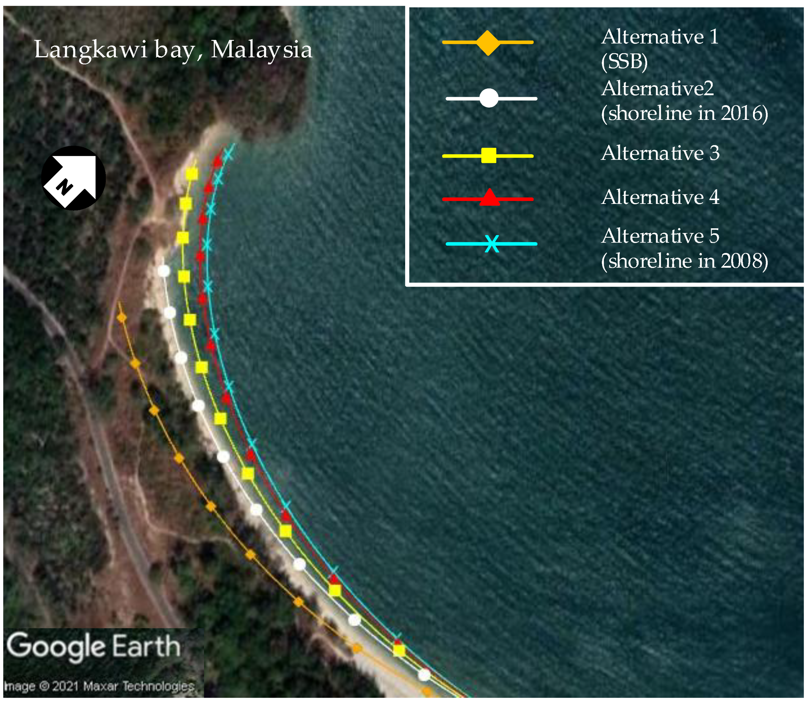
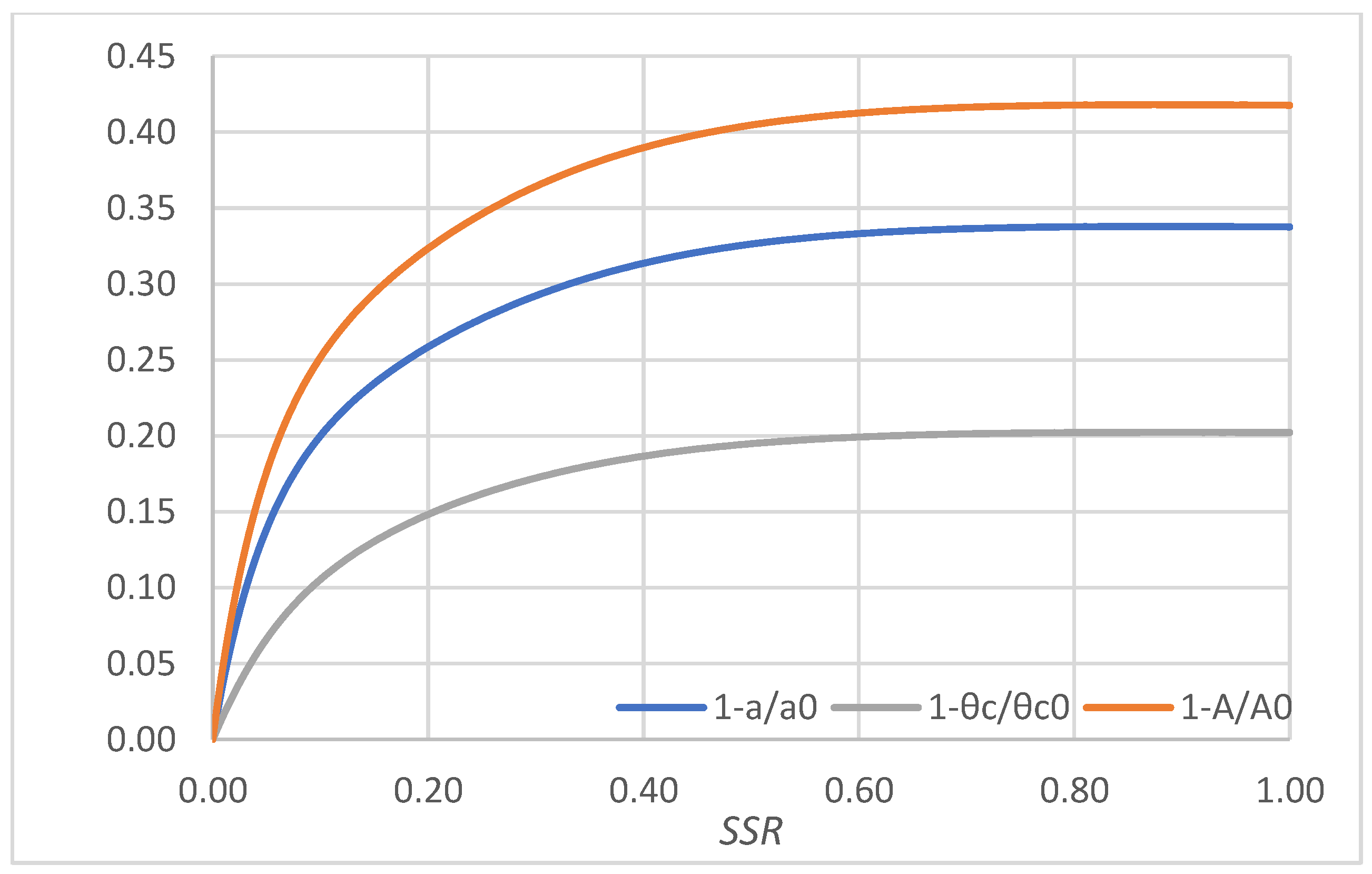
| Alternative | SSR | a (km) | θc (deg) | A (km2) | 1 − a/a0 | 1 − θc/θc0 | 1 − A/A0 |
|---|---|---|---|---|---|---|---|
| Alternative 1 (SSB) | 0.000 | 0.2693 | 112.08 | 0.1323 | 0.0000 | 0.0000 | 0.0000 |
| Alternative 2 (shoreline in 2016) | 0.100 | 0.2155 | 100.27 | 0.0990 | 0.2000 | 0.1054 | 0.2516 |
| Alternative 3 | 0.200 | 0.1997 | 95.47 | 0.0895 | 0.2586 | 0.1482 | 0.3235 |
| Alternative 4 | 0.400 | 0.1848 | 91.17 | 0.0807 | 0.3137 | 0.1866 | 0.3899 |
| Alternative 5 (shoreline in 2008) | 0.875 | 0.1783 | 89.40 | 0.0770 | 0.3380 | 0.2024 | 0.4182 |
Publisher’s Note: MDPI stays neutral with regard to jurisdictional claims in published maps and institutional affiliations. |
© 2022 by the authors. Licensee MDPI, Basel, Switzerland. This article is an open access article distributed under the terms and conditions of the Creative Commons Attribution (CC BY) license (https://creativecommons.org/licenses/by/4.0/).
Share and Cite
Manakul, C.; Mohanasundaram, S.; Weesakul, S.; Shrestha, S.; Ninsawat, S.; Chonwattana, S. Classifying Headland-Bay Beaches and Dynamic Coastal Stabilization. J. Mar. Sci. Eng. 2022, 10, 1363. https://doi.org/10.3390/jmse10101363
Manakul C, Mohanasundaram S, Weesakul S, Shrestha S, Ninsawat S, Chonwattana S. Classifying Headland-Bay Beaches and Dynamic Coastal Stabilization. Journal of Marine Science and Engineering. 2022; 10(10):1363. https://doi.org/10.3390/jmse10101363
Chicago/Turabian StyleManakul, Chayutpong, S. Mohanasundaram, Sutat Weesakul, Sangam Shrestha, Sarawut Ninsawat, and Somchai Chonwattana. 2022. "Classifying Headland-Bay Beaches and Dynamic Coastal Stabilization" Journal of Marine Science and Engineering 10, no. 10: 1363. https://doi.org/10.3390/jmse10101363
APA StyleManakul, C., Mohanasundaram, S., Weesakul, S., Shrestha, S., Ninsawat, S., & Chonwattana, S. (2022). Classifying Headland-Bay Beaches and Dynamic Coastal Stabilization. Journal of Marine Science and Engineering, 10(10), 1363. https://doi.org/10.3390/jmse10101363