Discrete Element Method Approach to Modeling Mechanical Properties of Three-Dimensional Ice Beams

Abstract

The mechanical properties of ice were numerically studied using the discrete element method (DEM). For ice beam simulations, an open-source DEM library was used. The uniaxial compression test and three-point bending test for modeled ice particles with a bond model were simulated. The mechanical properties of ice were dependent on the parameters of the contact model and the bond model. The bond model was applied to simulate the failure of ice. To model the Young’s modulus, flexural strength, and compressive strength of ice, the relationship with the model parameters of the contact and bonding models was investigated, and equations proposed. Real ice in the Bohai Sea was modeled using the proposed relational equations, and its mechanical properties were predicted. Simulated mechanical properties were compared with measured data in the Bohai Sea.

1. Introduction

In Arctic activity, the study of ice load due to the interaction of marine structures with sea ice plays a very important role. A range of experimental, analytical, and empirical approaches have been applied to estimating ice load. In general, experimental studies have been carried out through model tests in an ice basin, or through field tests [1,2]. Experimental studies have the advantage of obtaining the most reliable data, but involve significant time and costs, and there are limitations on the size and method of the test equipment [3]. Analytical and empirical approaches to predicting ice load due to ice–structure interaction have been proposed by many researchers [4,5]. Most studies have dealt with ice load in level ice. Hu and Zhou [6] used several popular empirical and analytical equations to predict the ice load of icebreakers in level ice. Jeong et al. [7] proposed a semi-empirical method based on Lindqvist’s model in level ice. However, since the analytical and empirical models were mostly based on simple linear relationships and ice models, it was difficult to extend them to real ice conditions [3].

With the advancement of computer modeling, many studies using numerical methods began to be conducted. Finite element method (FEM) has long been applied to ice–structure interaction issues by simulating collisions, deformations, and damage based on theoretical constitutive equations [8,9]. FEM was generally used to simulate local and global ice loads in various ice conditions, such as level ice, ice ridges, and icebergs [10,11]. The discrete element method (DEM) was suitable for modeling discrete ice and was used to simulate the interaction between pack ices and structures [12,13]. DEM was one of the techniques that could simulate ice and structure interaction problems, including ice breakage, broken ice behavior, and interactions between small ice blocks [14]. Furthermore, in recent years, DEM has been adopted to study the heat transfer of frozen soil and to establish a more detailed predictive model [15,16,17].

The ice load due to the interaction of the ice with structures is dependent on the mechanical properties of the ice. The mechanical properties of simulated ice were determined by the model parameters applied to the particles [18]. In a bond model, the typical model parameters were Young’s modulus of the bond, the ratio of the normal and tangential components of bond stiffness, the bond radius factor, the tensile bond strength, and the shear bond strength. In most studies using DEM, the optimal model parameters were determined through trial and error to model ice. Recently, to conduct ice–structure interaction studies, an increasing number of studies have sought to understand the relationship between model parameters and simulated mechanical properties of ice [19,20]. Ji et al. [19] analyzed the effect of the friction coefficient between particles and the bond strength of the bonded particles on the fracture process of sea ice through DEM simulation. The ratio of the compressive strength to the flexural strength was used to calibrate the bond strength and friction coefficient of bonded particles. Long et al. [20] simulated uniaxial compressive tests and three-point bending tests to study the relationship between the strength of sea ice and model parameters such as particles size, sample size, bond strength, and interparticle friction coefficient. The uniaxial compressive strength and flexural strength of sea ice increased as the size ratio increased. The arrangement of the particles constituting the ice and the relative size of the particles of the ice also significantly affected the mechanical properties of simulated ice. Although many researchers have attempted to establish the relationship between model parameters and mechanical properties through DEM simulation, these studies need to be further carried out in order to apply them to the complex ice and structure interaction problems [14].

In this study, a method for modeling the mechanical properties of ice was presented, and the coefficients affecting it were summarized. The mechanical properties of ice in the Bohai Sea were predicted using the proposed equations. For ice modeling, DEM with a bond model was used. For numerical analysis, an open-source DEM library solver was used [21]. Cantilever deflection was simulated to verify bond and contact models. A uniaxial compression test and a three-point bending test were simulated to study the effect of model parameters on the mechanical properties of ice. The mechanical properties of ice were compared with data from the Bohai Sea.

2. Numerical Modeling

2.1. Equations of Motion

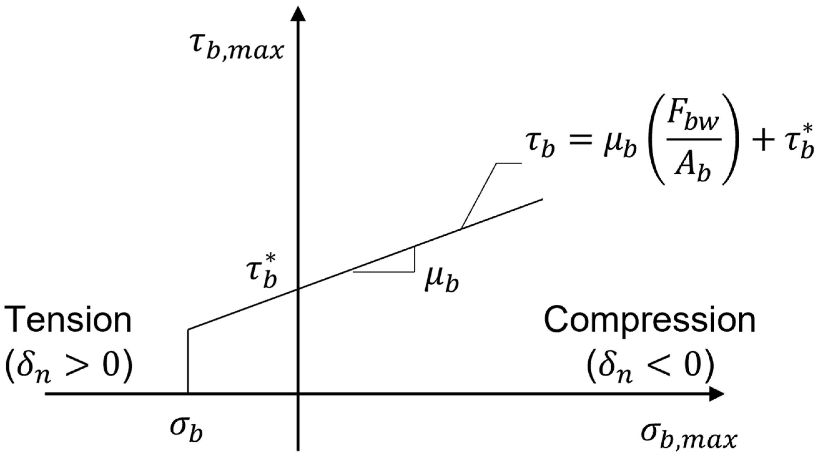
In DEM, the translational and rotational motions of an individual particle are governed by Newton’s second law, and are expressed as

$$m\frac{d\mathit{u}}{dt}={\displaystyle \sum }{\mathit{F}}_c+{\displaystyle \sum }{\mathit{F}}_b+{\mathit{F}}_g$$

(1)

$$I\frac{d\mathit{\omega }}{dt}={\displaystyle \sum }{\mathit{M}}_c+{\displaystyle \sum }{\mathit{M}}_b$$

(2)

where, the subscripts c and b denote contact and bond, respectively. $m$ is the particle mass, and $\mathit{u}$ is the particle velocity. ${\mathit{F}}_c$ and ${\mathit{F}}_b$ represent the particle contact force and the force due to the bond model, respectively. ${\mathit{F}}_g$ is the force due to gravity. $I$ is the particle moment of inertia and $\mathit{\omega }$ is the particle’s angular velocity. ${\mathit{M}}_c$ and ${\mathit{M}}_b$ represent the torque due to particle contact and the torque due to particle bonding, respectively. The contact between particles was simplified using the spring–dashpot model [21].

2.2. Bond Model

The bonding between particles was based on the parallel bond model [22]. Figure 1 shows two particles connected by a bond model. The bond model had a cylindrical shape characterized by a bond length ($l_b$) and a bond radius ($R_b$). The bond radius of the bond model was defined as ${\lambda }_{b}r$. Here, ${\lambda }_b$ is a radius factor. The subscripts $n$ and $t$ represent normal and tangential directions, respectively.

The forces and moments acting on the bond model include tension, compression, shear, torsion and bending moments, which were transmitted as forces and torques to the two connected particles. The forces and moments acting on the bond elements were expressed as follows.

$$\Delta {\mathit{F}}_{b,n}\left(t\right)=k_{b,n}{A}_b\Delta t\Delta {\mathit{u}}_n$$

(3)

$$\Delta {\mathit{F}}_{b,t}\left(t\right)=-k_{b,t}{A}_b\Delta t\Delta {\mathit{u}}_t$$

(4)

$$\Delta {\mathit{M}}_{b,n}\left(t\right)=-k_{b,t}{J}_b\Delta t\Delta {\mathit{\omega }}_n$$

(5)

$$\Delta {\mathit{M}}_{b,t}\left(t\right)=-k_{b,n}{I}_b\Delta t\Delta {\mathit{\omega }}_t$$

(6)

where, the subscripts $n$ and $t$ denote normal and tangential components, respectively. $k_b$ is the stiffness of the bond model. $A_b\left(=\pi R_b^2\right)$ is the cross-sectional area of the bond model, $J_b\left(=0.5\pi R_b^4\right)$ is the polar moment of inertia, and $I_b\left(=0.25\pi R_b^4\right)$ is the moment of inertia. $\Delta t$ represents the time interval. $k_{b,n}$ and $k_{b,t}$ could be expressed as

$$k_{b,n}=\frac{E_b}{l_b}$$

(7)

$$k_{b,t}=\frac{k_{b,n}}{{\lambda }_{ns}},$$

(8)

where, $E_b$ is the Young’s modulus in the bond model ($E_b$), and ${\eta }_b(=k_{b,n}/k_{b,t}$) is the ratio of the normal and tangential components of bond stiffness.

When the bond between particles was broken, excessive kinetic energy was released if the relative motion between the particles was large. This resulted in early failure of the ice, promoting the destruction of adjacent bonding particles [23]. Because this had a direct effect on the simulated ice strength, a damping model proportional to the relative velocity between the two particles was applied to the bond model [24]. The damping force ($F_{d,n}$, $F_{d,t}$) and the damping moment ($M_{d,n}$, $M_{d,t}$) can be expressed as follows.

$${\mathit{F}}_{d,n}\left(t\right)=-2{\gamma }_b{\left(M^{\ast }{k}_{b, n}{A}_b\right)}^{1/2}{\mathit{u}}_n$$

(9)

$${\mathit{F}}_{d,t}\left(t\right)=-2{\gamma }_b{\left(M^{\ast }{k}_{b,t}{A}_b\right)}^{1/2}{\mathit{u}}_t$$

(10)

$${\mathit{M}}_{d,n}\left(t\right)=-2{\gamma }_b{\left(J^{\ast }{k}_{b,n}{J}_b\right)}^{1/2}{\mathit{\omega }}_n$$

(11)

$${\mathit{M}}_{d,t}\left(t\right)=-2{\gamma }_b{\left(J^{\ast }{k}_{b,t}{I}_b\right)}^{1/2}{\mathit{\omega }}_t$$

(12)

where, $M^{\ast }$ and $J^{\ast }$ represent the effective mass and moment of inertia of the bonding particle, respectively. The bond damping constant (${\gamma }_b$) is the energy dissipation rate, and ranges from 0 to 1.

The failure of the bond model started when the maximum tensile stress or shear stress acting on the bond model exceeded the bond strength (${\sigma }_b$) or shear bond strength (${\tau }_b$), as shown in the following equation.

$${\sigma }_{b,max}>{\sigma }_b\mathrm{or}{\tau }_{b,max}>{\tau }_b$$

(13)

The failure of the bond model was modeled using the elastic beam theory. The strength of the bond model was defined as the maximum value of the normal and shear stresses, as

$${\sigma }_{b,max}=-\frac{{\mathit{F}}_{b,n}}{A_b}+\frac{\left|{\mathit{M}}_{b,t}\right|R_b}{I_b}$$

(14)

$${\tau }_{b,max}=\frac{\left|{\mathit{F}}_{b,t}\right|}{A_b}+\frac{\left|{\mathit{M}}_{b,n}\right|R_b}{J_b}$$

(15)

The normal stress acting on the bond model can be divided into the compressive stress and the tensile stress. A negative sign in the normal stress means that the bond was broken only by the tensile stress. In the tensile state, the distance between the centers of two particles (${\delta }_n$) was greater than the radius of the two particles ($2r$), and failure occurred due to normal and shear stresses. On the other hand, in the compressed state, the distance between the centers of two particles (${\delta }_n$) was smaller than the radius of the two particles ($2r$), and failure only occurred due to shear stress.

Ice is treated as a brittle material such as rock or concrete [19]. To model the failure of ice, the Mohr–Coulomb failure criterion was used as the failure criterion of the bond model [20]. Figure 2 shows the failure envelope of the bond model according to the Mohr–Coulomb failure criterion. The shear bond strength (${\tau }_b$) was calculated using the following equation.

$${\tau }_b={\mu }_b\left(\frac{F_{b,n}}{A_b}\right)+{\tau }_b^{\ast }$$

(16)

where, the first term on the right side represents the frictional force in the bond model due to the normal stress. ${\mu }_b$ is the bond friction coefficient and $F_{b,n}/A_b$ is the force in the normal direction acting on the bond model. The second term is the shear strength when the bond friction coefficient is zero, which corresponds to cohesion. The pure shear bond strength (${\tau }_b^{\ast }$) is a model variable.

Before the bond model connecting the two particles was broken, the only force considered to be acting on the particle was the force of the bond model. When the bond model was broken, the bond model connecting the particles was removed, and a force from the contact model was applied to the two particles.

2.3. Model Parameters

The mechanical properties of simulated ice were dominated by the stiffness and strength of the bond model. To understand the relationship between the mechanical properties of ice and the model parameters, the bond Young’s modulus ($E_b$), the bond strength (${\sigma }_b$), the pure shear bond strength (${\tau }_b^{\ast }$), the bond stiffness ratio of normal and tangential components (${\eta }_b$), the bond radius ($R_b$) and the bond friction coefficient (${\mu }_b$) were considered. The pure shear bond strength (${\tau }_b^{\ast }$) was applied in the same manner as the bond strength (${\sigma }_b$). Relative particle size ($L/d$) was used to investigate the effect of particle size on specimen size. $L$ represented the smallest dimension of the specimen, and $d$ was the particle diameter. Particle Poisson’s ratio ($\nu$), density ($\rho$), coefficient of restitution ($e$), and friction coefficient ($\mu$) did not significantly affect the mechanical properties of simulated ice, so the same values were applied to all simulations.

Table 1. Summary of simulation parameters.

Parameter	Value
Particle Poisson’s ratio [ν]	0.3
Particle friction coefficient [μ]	0.015
Relative particle size (L/d)	3.60, 7.06, 13.99, 27.85
Number of particles layers across L	4, 6, 8, 10, 12
Particle density (ρ) [kg/m3]	920
Coefficient of restitution (e)	0.1
$\mathrm{Bond}\mathrm{Young}’\mathrm{s}\mathrm{modulus}(E_b$) [GPa]	1.0, 2.0, 3.0
Bond friction coefficient (${\mu }_b$)	0, 0.1, 0.2, 0.3
Bond stiffness ratio (${\eta }_b$)	1.0, 2.0, 3.0
$\mathrm{Bond}\mathrm{radius}\mathrm{factor}({\lambda }_b)$	0.9
Bond strength (σb) [MPa]	0.5, 0.75, 1.0, 1.5, 2.0

shows the principal model parameters for ice modeling.

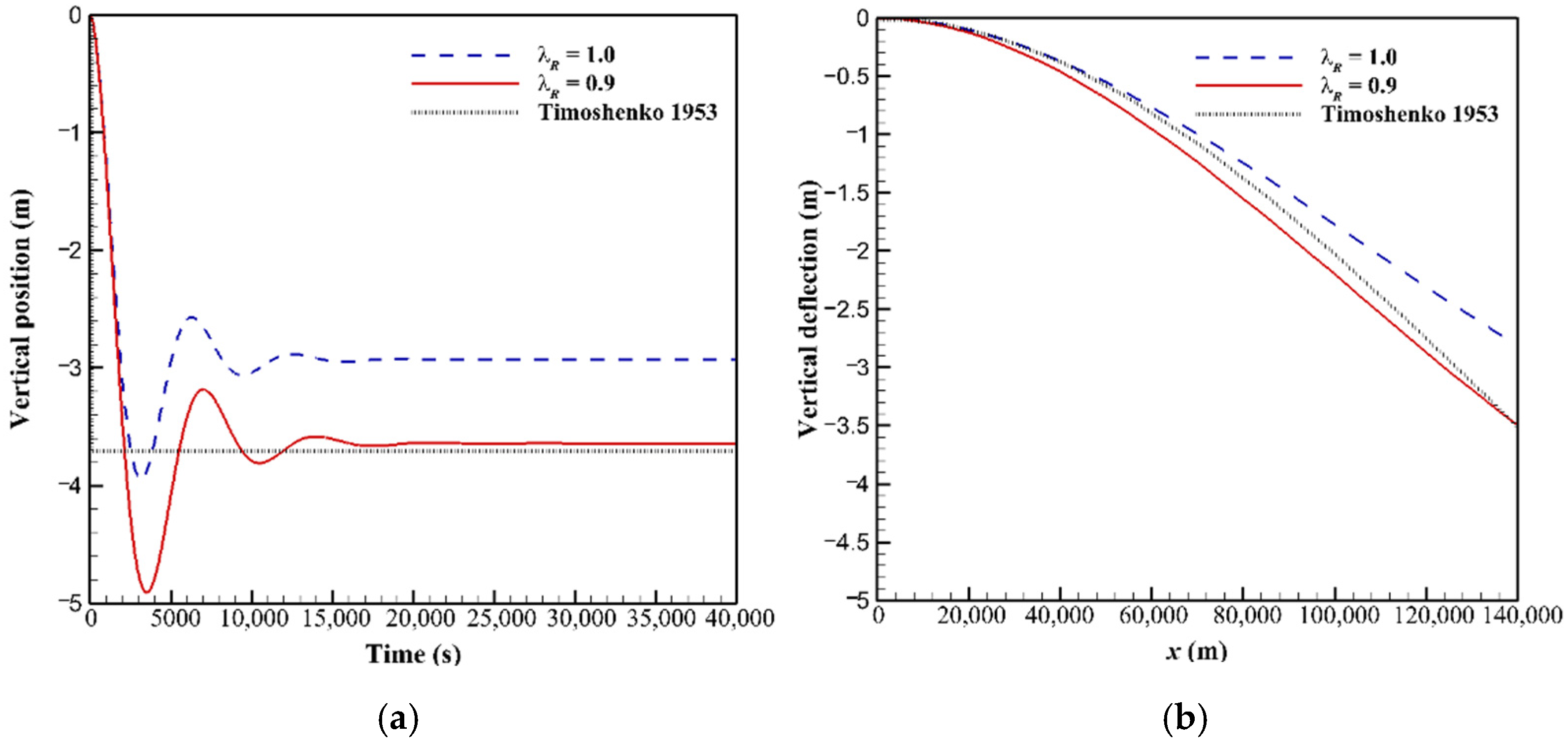
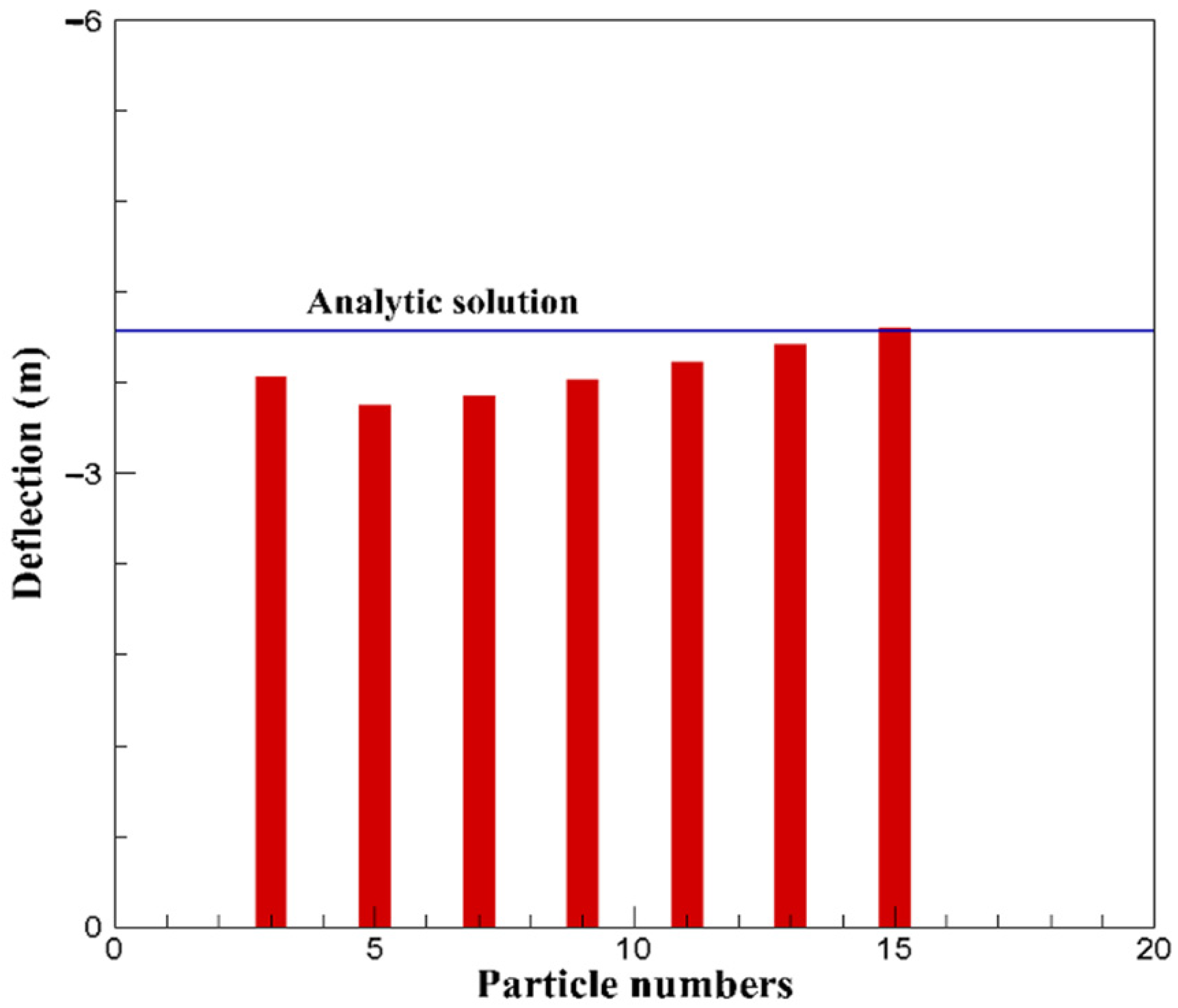
2.4. Model Verification

To verify the bond model, the cantilever beam deflection was simulated. Figure 3 shows the schematic for the simulation. The cantilever beam size ($h\times b\times L$) was 15,000 m × 15,000 m × 150,000 m. The cantilever beam was composed of particles with the same particle size and density bonded to each other. The particle arrangement was a simple cubic form [25], and the same number of particles was applied in the height ($h$) and width ($b$) directions. To simulate the cantilever beam deflection, the gray particles at the left end were fixed. The gray particles were constrained in translation and rotational motion. A concentrated load ($P=1.5\times {10}^{10}$ N) acted vertically on the upper middle red particle at the right end of the beam. The bond strength was set to a very high value in order to ignore failure of the bond model.

The deflection ($\delta$) of the cantilever beam was calculated based on the cantilever beam end, and the theoretical solution could be obtained by the following formula [26]:

$$\delta \left(x\right)=-\frac{P{x}^2\left(3l-x\right)}{6EI}$$

(17)

Figure 4 shows the deflection for various radius factors. When the load was applied, the end of the beam sagged rapidly and vibrated up and down. However, due to the damping force, the vibration amplitude decreased and reached an equilibrium state [25]. The simulation results showed a smaller deflection than the theoretical solution. A relatively smaller deflection occurred when the radius factor (${\lambda }_b$) was 1 compared to when it was 0.9. Because the force and moment acting on the bond model were proportional to the cross-sectional area ($A_b$), the higher the radius factor (${\lambda }_b$), the greater the resistance force. When the radius factor (${\lambda }_b$) was 0.9, resistance to the external force was reasonably generated.

Figure 5 shows the simulation results according to the number of particles of cantilever beams. Because the height ($h$) was fixed, the larger the particle sizes, the smaller the number of particles. Except when the number of particles was 3, the simulation results were consistent with the theoretical solution as the particle size was relatively small.

3. Results and Discussion

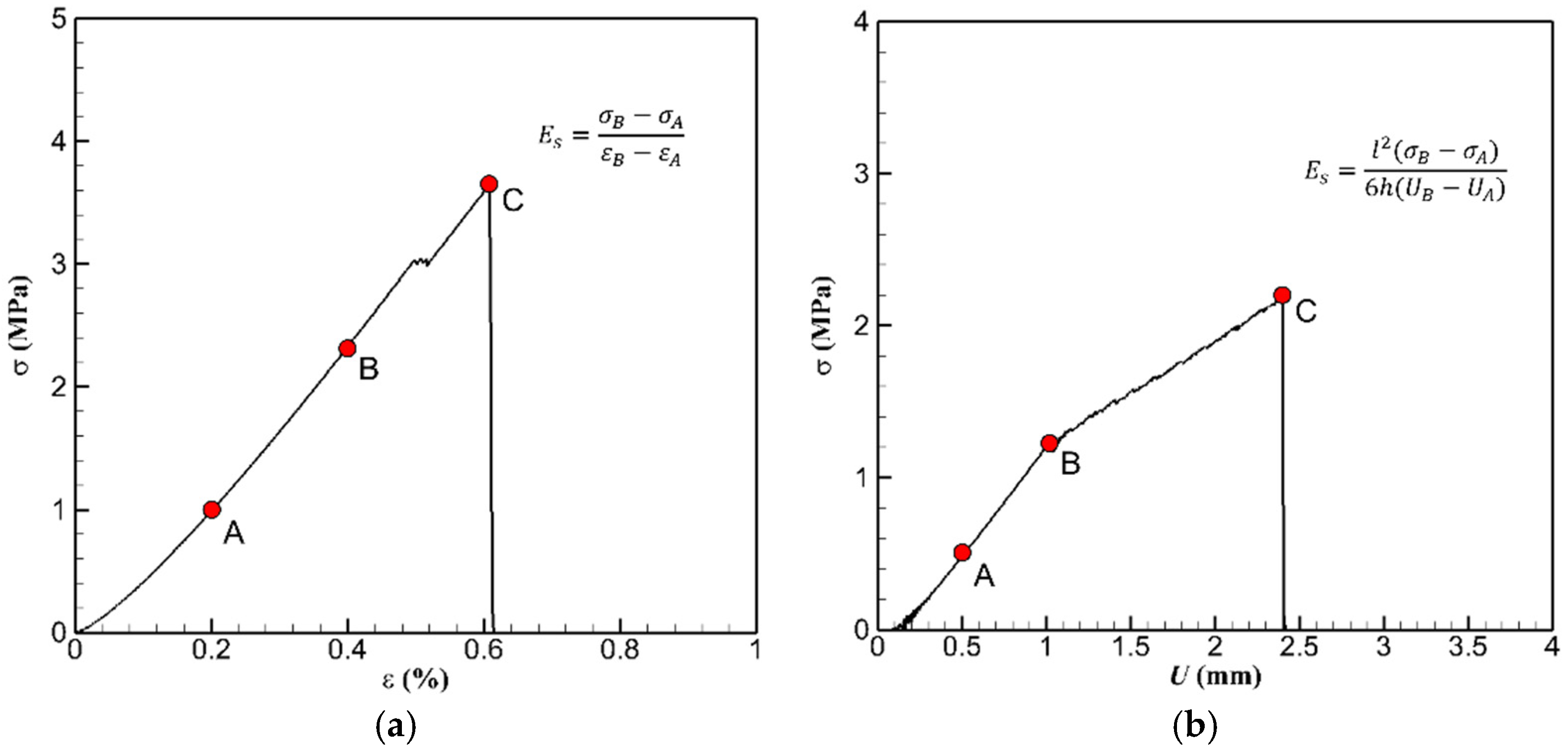
3.1. Uniaxial Compressive Test and Three-Point Bending Test

Uniaxial compressive tests and three-point bending tests were performed to determine the effect of model parameters on the simulated Young’s modulus ($E_s$), compressive strength (${\sigma }_c$), and flexural strength (${\sigma }_f$) of ice. To create the specimen, the particle array was configured with hexagonal close packing (HCP) [21]. Figure 6 shows the configuration and the size of the ice specimens. The size of the specimen used for the uniaxial compression test ($b_1\times h_1\times l_1$) was 100 mm $\times$ 100 mm $\times$ 250 mm. The ice specimen was supported by the bottom plate and the top plate as initial conditions. With the progress of time, the bottom plate was fixed and the top plate moved vertically downward at a constant speed of 0.005 m/s. For the three-point bending test ($b_2\times h_2\times l_2$), the size of the specimen was 70 mm × 70 mm × 700 mm. As an initial condition for the ice specimen, two support bars were placed at the bottom and a load bar was placed at the top. The distance ($l_2$) between the two support bars at the bottom was 500 mm, and the load bar at the top was placed in the center of the specimen. With the progress of time, the upper load bar moved vertically downward at a constant speed of 0.005 m/s, and the two support bars were fixed.

Figure 7 shows the failure of the simulated specimen. In the simulations, the Young’s modulus ($E_b$) of the bond was 1.0 GPa, the bond’s strength (${\sigma }_b$) was 1.0 MPa, the bond’s stiffness ratio (${\eta }_b$) was 2.0, the bond’s friction coefficient (${\mu }_b$) was 0, and the relative particle size ($L/d$) was 7.06. L was 100 mm and d was 14.16 mm in the uniaxial compression test, and L was 70 mm and d was 9.92 mm in the three-point bending test. Figure 7a shows the failure of the uniaxial compression test. The result showed a shear failure pattern with cracks occurring at the lower end of the specimen [27]. Figure 7b shows the failure of the three-point bending test. The result showed a tensile failure pattern with vertical cracks occurring in the bottom center of the specimen [20]. The failure of the simulated specimens well described the patterns seen in the testing of real ice specimens.

Figure 8 shows the stress–strain curve and the stress–deflection curve obtained from the simulation. In the stress–strain curve of the uniaxial compressive test, the stress increases linearly in the initial stage. When the strain was around 0.48%, initial cracks occurred due to the failure of the bond model. As a result, the stress decreased slightly after the initial crack was started. Then the stress increased almost linearly, but at a lower rate than in the initial stage. When the stress reached the compressive strength, the ice specimen failed. The same applies to the three-point bending test. In the uniaxial compressive test and the three-point bending test, the simulated Young’s modulus ($E_s$) of ice was calculated as follows, respectively.

$$E_s=\frac{\left({\sigma }_B-{\sigma }_A\right)}{\left({\epsilon }_B-{\epsilon }_A\right)}\mathrm{for}\mathrm{compressive}\mathrm{test}$$

(18)

$$E_s=\frac{l^2}{6h}\frac{\left({\sigma }_B-{\sigma }_A\right)}{\left(U_B-U_A\right)}\mathrm{for}\mathrm{three}-\mathrm{point}\mathrm{bending}\mathrm{test}$$

(19)

where, the subscripts A, B and C mean any three points selected from the stress–strain curve in the uniaxial compression test and the stress–deflection curve in the three-point bending test. $\sigma$, $\epsilon$ and $U$ represent stress, strain, and deflection, respectively.

In the uniaxial compressive test and the three-point bending test, the compressive strength (${\sigma }_c$) and the flexural strength (${\sigma }_f$) were respectively calculated as follows.

$${\sigma }_c=\frac{P_{max}}{bh}$$

(20)

$${\sigma }_f=\frac{3}{2}\frac{P_{max}l}{b{h}^2}$$

(21)

where, $P_{max}$ is the maximum load applied to the ice specimen. In the uniaxial compressive test, the simulated Young’s modulus and compressive strength of the ice specimens were 0.64 GPa and 3.65 MPa, respectively. In the three-point bending test, they were 0.86 GPa and 2.18 MPa, respectively. The obtained ratio of compressive strength to flexural strength (${\sigma }_c/{\sigma }_f$) was 1.67, which was small compared to 2.37, which was the average value of the ratio of compressive strength to flexural strength of actual ice measured in the Bohai Sea [19,28]. In the Mohr–Columb failure criterion, the shear bond strength (${\tau }_b$) was determined by the compressive strength including the bond friction coefficient (${\mu }_b$). The ratio of compressive strength to flexural strength (${\sigma }_c/{\sigma }_f$) was affected by the bond friction coefficient [19]. It appeared to be different from the measurement data of the Bohai Sea because the model parameters including the bond friction coefficient were not sufficiently considered.

3.2. Effect of Bond Young’s Moduls

Figure 9 shows the simulation results for Young’s modulus ($E_b$) of three bonds. The slope of the strain and deflection curves increased as the bond Young’s modulus increased. On the other hand, the maximum stress of the ice specimen decreased very slightly as the bond’s Young’s modulus increased. The bonds’ Young’s modulus had little effect on the simulated compressive strength and flexural strength. Figure 9c shows the relationship of the simulated Young’s modulus to the bonds’ Young’s modulus. The simulated Young’s modulus increased linearly with respect to the bonds’ Young’s modulus. In the uniaxial compression test, the ratio between the simulated Young’s modulus and the bonds’ Young’s modulus was 0.8, and the ratio was 0.57 in the three-point bending test. In the contact model, the spring stiffness based on the Hertz model [29] was non-linear with respect to the overlap length ($\delta$). For very small overlap lengths, a low spring stiffness was observed. This feature was more pronounced in the uniaxial compression test in which the contact was dominant [30]. Therefore, the simulated Young’s modulus ratio ($E_s/E_b$) for the uniaxial compression test showed a lower value than that of the three-point bending test.

A bending test was more commonly performed to measure the Young’s modulus of ice [31]. Figure 10 shows the ratio of Young’s modulus ($E_s/E_b$) to relative particle size in the three-point bending test. The ratio of Young’s modulus also increased as the relative particle size increased. If the ratio of Young’s modulus was less than one, it indicated that ice failed at deformations larger than the target mechanical property. The ratio of the Young’s modulus to the relative particle size could be expressed by the following equation:

$$\frac{E_s}{E_b}=0.0048{\left(\frac{L}{d}\right)}^3-0.1018{\left(\frac{L}{d}\right)}^2+0.7219\left(\frac{L}{d}\right)-0.8355$$

(22)

3.3. Effect of Bond Strength

Figure 11 shows the simulation results for various bond strengths. As the bond strength increased, the compressive strength and flexural strength increased. The initial slope of the strain curve was constant because the bond strength did not affect the simulated Young’s modulus ($E_s$). The compressive strength (${\sigma }_c$) and flexural strength (${\sigma }_f$) increased linearly with the bond strength, and the simulated strength ratios to the bond strength were obtained. As the relative particle size increased, the strength ratio (${\sigma }_c/{\sigma }_b, {\sigma }_f/{\sigma }_b$) also increased.

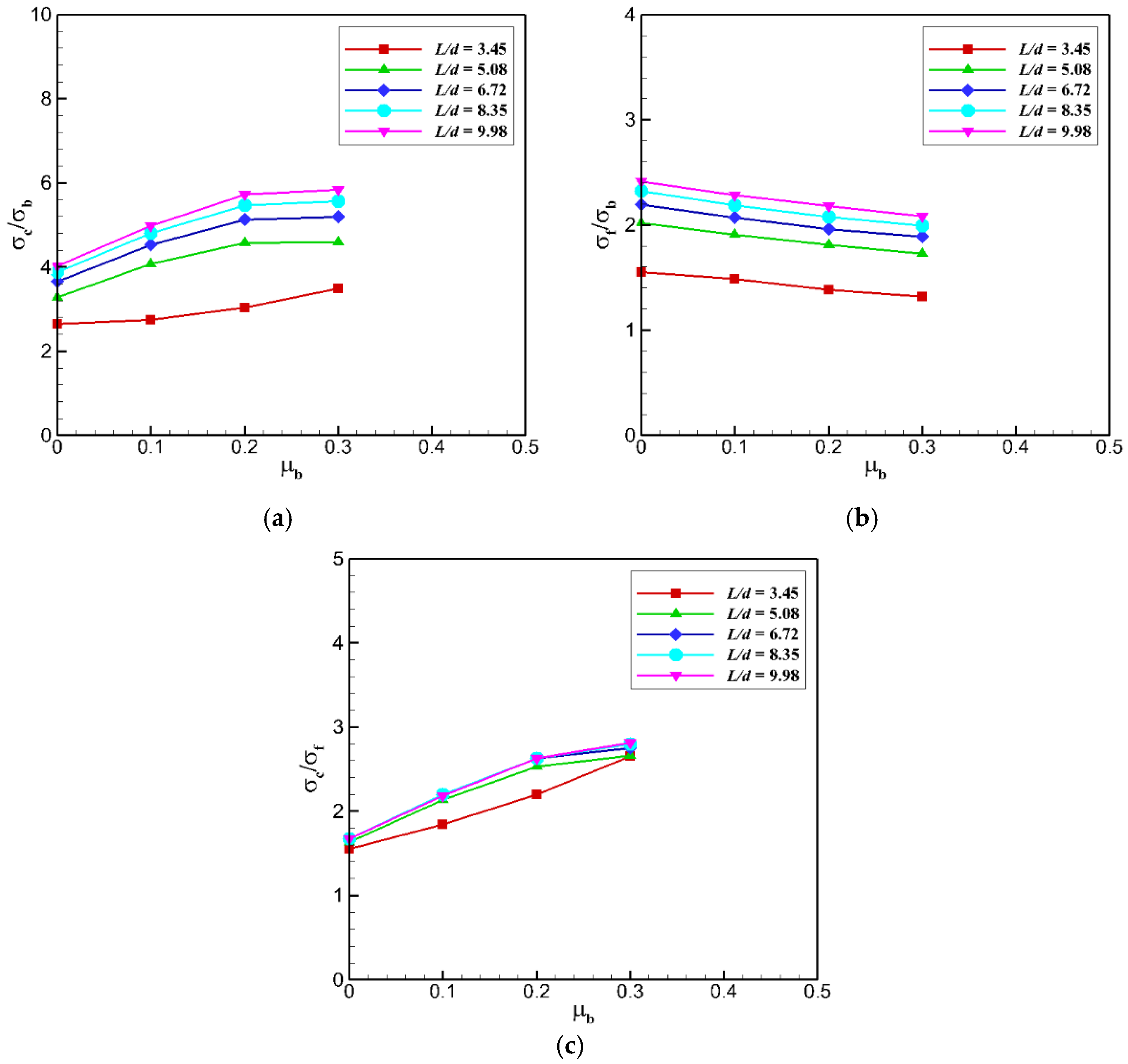
3.4. Effect of Bond Friction Coefficient

Figure 12 shows the simulation results for various bond friction coefficients (${\mu }_b$). The compressive strength of ice increased at a constant rate until the bond friction coefficient was 0.2. When the bond friction coefficient was 0.3, the rate of increase decreased. As the bond friction coefficient increased, the compressive strength increased while the flexural strength decreased. This meant that the effect of the bond friction coefficient on the ice strength according to the load conditions was opposite.

In the uniaxial compression test, the particles were in compression. The shear bond strength (${\tau }_b$) increased as the bond friction coefficient increased. Because only shear failure was considered in compression, as the bond friction coefficient increased, the resistance to shear failure increased and the compressive strength of ice increased. In the three-point bending test, the particles were in tension. The shear bond strength decreased as the bond friction coefficient increased. As the bond friction coefficient increased, the resistance to shear failure decreased and the flexural strength of ice decreased.

Figure 13 shows the failure pattern of the ice specimen for various bond friction coefficients in the uniaxial compression test. Shear failure occurred at the lower end of the specimen, and the shear failure angle increased as the bond friction coefficient increased. This proved that the bond friction coefficient well reproduced the friction angle in the Mohr–Coulomb failure criterion. On the other hand, shear failure occurred at the upper end of the specimen when the bond friction coefficient was 0.3 because the bond friction coefficient did not properly reproduce the friction angle, as the resistance to shear failure increased more than necessary.

Figure 14 shows the effect of relative particle size for various bond friction coefficients. The compressive and tensile strengths for the bond friction coefficient increased as the relative particle size increased. As the relative particle size increased, the simulated ice strength ratio (${\sigma }_c/{\sigma }_b, {\sigma }_f/{\sigma }_b$) also increased. The compressive strength ratio (${\sigma }_c/{\sigma }_b$) had a small effect when the bond friction coefficient was 0.3 or more. As the bond friction coefficient increased, the compressive strength ratio (${\sigma }_c/{\sigma }_b$) increased, and conversely, the flexural strength (${\sigma }_f/{\sigma }_b$) ratio decreased. The compression and flexural strength ratio (${\sigma }_c/{\sigma }_f$) maintained almost constant values when the relative particle size was five or more.

Figure 15 shows the bond friction coefficient for various relative particle sizes. The ratio of flexural strength to bond strength showed a linear relation with respect to the bond friction coefficient. The ratio of compression strength to flexural strength also showed a behavior that was close to linear. The compressive strength ratio and the flexural strength ratio of simulated ice for the bond friction coefficient could respectively be expressed as follows.

$$\frac{{\sigma }_c}{{\sigma }_b}=A_c{\mu }_b+B_c$$

(23)

$$\frac{{\sigma }_f}{{\sigma }_b}=A_f{\mu }_b+B_f$$

(24)

The coefficients of $A_c$, $B_c$, $A_f$, and $B_f$ could be expressed in the function of the relative particle size, respectively, as follows.

$$A_c=0.3202\frac{L}{d}+4.6827$$

(25)

$$B_c=-0.0144{\left(\frac{L}{d}\right)}^2+0.3815\left(\frac{L}{d}\right)+1.5533$$

(26)

$$A_f=0.0649\frac{L}{d}+1.6466$$

(27)

$$B_f=0.0021{\left(\frac{L}{d}\right)}^3-0.0427{\left(\frac{L}{d}\right)}^2+0.2268\left(\frac{L}{d}\right)-1.304$$

(28)

The equation for the strength ratio to the bond friction coefficient could be formulated as follows.

$$\frac{{\sigma }_c}{{\sigma }_f}=4.7167{\mu }_b+1.673$$

(29)

The ratio of compressive strength to flexural strength (${\sigma }_c/{\sigma }_f$) was in the range of 1.66 to 2.6. This range included the average value of 2.37 and the maximum value of 2.47 of actual sea ice measured in the Bohai Sea [19,28].

3.5. Effect of Bond Stiffness Ratio (${\eta }_b$)

Figure 16 shows the effect of the bond stiffness ratio of normal and tangential components (${\eta }_b$). The bond stiffness ratio affected both the simulated Young’s modulus and strength of the simulated ice. As the bond stiffness ratio increased, the simulated Young’s modulus ratio ($E_s/E_b$) showed a decreasing trend [18]. Since the tangential bond stiffness ($k_{b,t}$) was inversely proportional to the bond stiffness ratio, as the bond stiffness ratio increased, the tangential bond stiffness decreased. As the bond stiffness ratio increased, the increment of the tangential force acting on the bond model decreased, and thus the simulated Young’s modulus of the simulated ice also decreased. As the bond stiffness ratio increased, the compressive strength and flexural strength increased, but when the bond stiffness ratio was five or more, the compressive strength and flexural strength decreased. When the bond stiffness ratio was three or less, the ratio of compressive strength to flexural strength (${\sigma }_c/{\sigma }_f$) was about 1.67. Therefore, a constant value of the bond stiffness ratio (${\eta }_b$) of two was selected to minimize the parameters affecting the mechanical properties of the ice.

3.6. Prediction of Mechanical Property of Ice in the Bohai Sea

The simulated compressive and flexural strengths were compared with those of Bohai Sea ice [28]. The measured average and maximum values of the compressive strengths were 2.56 MPa and 5.98 MPa, respectively. The measured average and maximum values of the flexural strengths were 1.08 MPa and 2.42 MPa, respectively. The average and maximum values of the ratio of compressive strength to flexural strength were 2.37 and 2.47, respectively.

The relative particle sizes were considered to be 5.08 and 8.35. From Equation (22), the bond Young’s modulus was applied equally to 1.2. The bond friction coefficient (${\mu }_b$) was calculated using Equation (29), and 0.15 and 0.17 were obtained for the average and maximum strength ratios, respectively.

Table 2. Parameters for ice simulation of the Bohai Sea.

Parameter	Three-Point Bending	Uniaxial Compressive
Particle Poisson’s ratio [ν]	0.3	0.3
Particle friction coefficient [μ]	0.015	0.015
Relative Particle size (L/d)	5.08, 8.35	5.08, 8.35
Particle density (ρ) [kg/m3]	920	920
Coefficient of restitution (e)	0.3	0.3
Time step (Δt) [s]	2.0 × 10−6	2.0 × 10−6
$\mathrm{Bond}\mathrm{Young}’\mathrm{s}\mathrm{modulus}(E_b$) [GPa]	1.2	1.2
$\mathrm{Bond}\mathrm{friction}\mathrm{coefficient}({\mu }_b$)	0.15, 0.17	0.15, 0.17
$\mathrm{Bond}\mathrm{stiffness}\mathrm{ratio}({\eta }_b$)	2.0	2.0
$\mathrm{Bond}\mathrm{radius}\mathrm{factor}({\lambda }_b$)	0.9	0.9
Bond strength (σb) for mean [MPa]	0.58, 0.51	0.60, 0.50
Bond strength (σb) for maximum [MPa]	1.31, 1.15	1.35, 1.14

shows the model parameters used in ice simulation. Figure 17 shows the stress–strain curve and the stress–deflection curve obtained from the simulation.

Table 3. Compressive strength and flexural strength in the Bohai Sea.

L/d		$\mathbf{Flexural}\mathbf{Strength}\left({\mathit{\sigma }}_{\mathit{f}}\right)$			$\mathbf{Compressive}\mathbf{Strength}\left({\mathit{\sigma }}_{\mathit{c}}\right)$
		Present	Bohai Sea (Ji et al. [28])	Difference (%)	Present	Bohai Sea (Ji et al. [28])	Difference (%)
5.08	Mean	1.07	1.08	−0.53	2.75	2.56	7.76
	Max	2.42	2.42	0.03	6.18	5.98	3.39
8.35	Mean	1.04	1.08	−3.58	2.74	2.56	7.06
	Max	2.39	2.42	−1.20	6.22	5.98	4.02

lists the compressive and flexural strengths of simulated ice. The simulated ice strength was close to the actual ice strength. The simulated compressive strength was predicted to be slightly higher because the bonds’ Young’s modulus in the uniaxial compression test was lower than the bonds’ Young’s modulus required to obtain the target Young’s modulus. From Figure 17 and Table 3, it could be seen that the model parameters obtained in Equations (22)–(29) well simulated the mechanical properties of ice.

4. Conclusions

Simulations of a uniaxial compression test and a three-point bending test of ice specimens were performed using DEM. For the simulations, the open-source DEM library solver was used [21]. The relationship between the mechanical properties of simulated ice and the model parameters was investigated. This relationship was very important for predicting the ice load caused by interaction with ice.

Ice was modeled using a bond model to simulate the failure of ice. In the bond model, Mohr–Coulomb failure criteria and bond strength were applied. To validate the bond model, the cantilever test was simulated and the size of the bonding model was determined.

To determine the model parameters affecting the mechanical properties of ice, various bond Young’s modulus, bond strength, bond friction coefficient, bond stiffness ratio, and relative particle size were considered. The simulated Young’s modulus of ice increased in proportion to the bond Young’s modulus. On the other hand, the simulated ice strength was not affected by the bond Young’s modulus, because the bond Young’s modulus was proportional only to the bond stiffness. The simulated strength ratio to bond strength increased with relative particle size. The simulated Young’s modulus of the simulated ice was not affected by the bond strength. According to the Mohr–Coulomb failure criterion, as the bond friction coefficient increased, the compressive strength increased while the flexural strength decreased. The effect of the bond friction coefficient on the simulated ice was reversed based on the load conditions according to the Mohr–Coulomb failure criterion. That is, as the bond friction coefficient increased, the compressive strength increased while the flexural strength decreased. From the study on the model parameter, the equations between the bond friction coefficient, the relative particle size, and the simulated ice strength were proposed. The model parameters obtained from the equations were used to simulate and predict the mechanical properties of real ice in the Bohai Sea. The predicted strengths were quite similar to those of actual ice measured in the Bohai Sea.

References

1. Huang, Y.; Sun, J.Q.; Ji, S.P. Experimental study on the resistance of a transport ship navigating in level Ice. J. Mar. Sci. Appl. 2016, 15, 105–111. [Google Scholar] [CrossRef]
2. Lee, S.C.; Park, S.; Choi, K.; Jeong, S.-Y. Prediction of ice loads on Korean IBRV ARAON with 6-DOF inertial measurement system during trials of Chukchi and East Siberian Seas. Ocean Eng. 2018, 151, 23–32. [Google Scholar] [CrossRef]
3. Ni, B.Y.; Chen, Z.W.; Zhong, K.; Li, X.A.; Xue, Y.Z. Numerical simulation of a polar ship moving in level ice based on a one-way coupling method. J. Mar. Sci. Eng. 2020, 8, 692. [Google Scholar] [CrossRef]
4. Lindqvist, G. A straightforward method for calculation of ice resistance of ships. In Proceedings of the 10th International Conference on Port and Ocean Engineering under Arctic Conditions (POAC), Luleå, Sweden, 12–16 June 1989; pp. 722–735. [Google Scholar]
5. Riska, K.; Wilhelmson, M.; Englund, K.; Leiviskä, T. Performance of Merchant Vessels in the Baltic; Research Report No. 52; Ship Laboratory, Helsinki University of Technology: Espoo, Finland, 1997. [Google Scholar]
6. Hu, J.; Zhou, L. Experimental and numerical study on ice resistance for icebreaking vessels. Int. J. Nav. Archit. 2015, 7, 626–639. [Google Scholar] [CrossRef]
7. Jeong, S.Y.; Choi, K.; Kang, K.J.; Ha, J.S. Prediction of ship resistance in level ice based on empirical approach. Int. J. Nav. Archit. 2017, 9, 613–623. [Google Scholar] [CrossRef]
8. Kuutti, J.; Kolari, K.; Marjavaara, P. Simulation of ice crushing experiments with cohesive surface methodology. Cold Reg. Sci. Technol. 2013, 92, 17–28. [Google Scholar] [CrossRef]
9. Liu, Z.; Amdahl, J.; Løset, S. Plasticity based material modelling of ice and its application to ship–iceberg impacts. Cold Reg. Sci. Technol. 2011, 65, 326–334. [Google Scholar] [CrossRef]
10. Aksnes, V. A simplified interaction model for moored ships in level ice. Cold Reg. Sci. Technol. 2010, 63, 29–39. [Google Scholar] [CrossRef]
11. Zhou, L.; Su, B.; Riska, K.; Moan, T. Numerical simulation of moored structure station keeping in level ice. Cold Reg. Sci. Technol. 2012, 71, 54–66. [Google Scholar] [CrossRef]
12. Yulmetov, R.; Løset, S. Validation of a numerical model for iceberg towing in broken ice. Cold Reg. Sci. Technol. 2017, 138, 36–45. [Google Scholar] [CrossRef]
13. Liu, L.; Ji, S. Ice load on floating structure simulated with dilated polyhedral discrete element method in broken ice field. Appl. Ocean Res. 2018, 75, 53–65. [Google Scholar] [CrossRef]
14. Tuhkuri, J.; Polojärvi, A. A review of discrete element simulation of ice–structure interaction. Philos. Trans. R. Soc. Math. Phys. Eng. Sci. 2018, 376, 20170335. [Google Scholar] [CrossRef] [PubMed]
15. El Shamy, U.; de Leon, O.; Wells, R. Discrete element method study on effect of shear-induced anisotropy on thermal conductivity of granular soils. Int. J. Geomech. 2013, 13, 57–64. [Google Scholar] [CrossRef]
16. Farahani, M.V.; Hassanpouryouzband, A.; Yang, J.; Tohidi, B. Heat transfer in unfrozen and frozen porous media: Experimental measurement and pore-scale modeling. Water Resour. Res. 2020, 56, e2020WR027885. [Google Scholar]
17. Farahani, M.V.; Hassanpouryouzband, A.; Yang, J.; Tohidi, B. Insights into the climate-driven evolution of gas hydrate-bearing permafrost sediments: Implications for prediction of environmental impacts and security of energy in cold regions. RSC Adv. 2021, 11, 14334–14346. [Google Scholar] [CrossRef]
18. Yang, B.; Jiao, Y.; Lei, S. A study on the effects of microparameters on macroproperties for specimens created by bonded particles. Eng. Comput. 2006, 23, 607–631. [Google Scholar] [CrossRef]
19. Ji, S.; Di, S.; Long, X. DEM simulation of uniaxial compressive and flexural strength of sea ice: Parametric study. J. Eng. Mech. 2016, 143, C4016010. [Google Scholar] [CrossRef]
20. Long, X.; Ji, S.; Wang, Y. Validation of microparameters in discrete element modeling of sea ice failure process. Part. Sci. Technol. 2018, 37, 550–559. [Google Scholar] [CrossRef]
21. Song, S.; Jeon, W.; Park, S. Parametric Study on Strength Characteristics of Two-Dimensional Ice Beam Using Discrete Element Method. Appl. Sci. 2021, 11, 8409. [Google Scholar] [CrossRef]
22. Potyondy, D.O.; Cundall, P.A. A bonded-particle model for rock. Int. J. Rock Mech. Min. Sci. 2004, 41, 1329–1364. [Google Scholar] [CrossRef]
23. Hazzard, J.F.; Young, R.P.; Maxwell, S.C. Micromechanical modeling of cracking and failure in brittle rocks. J. Geophys. Res. Solid Earth. 2000, 105, 16683–16697. [Google Scholar] [CrossRef]
24. Guo, Y.; Curtis, J.; Wassgren, C.; Ketterhagen, W.; Hancock, B. Granular shear flows of flexible rod-like particles. AIP Conf. Proc. 2013, 1542, 491–494. [Google Scholar]
25. Wang, M. A scale-invariant bonded particle model for simulating large deformation and failure of continua. Comput. Geotech. 2020, 126, 103735. [Google Scholar] [CrossRef]
26. Timoshenko, S.P. History of Strength of Materials; McGraw-Hill: New York, NY, USA, 1953; ISBN 9780070647251. [Google Scholar]
27. Zhang, N.; Zheng, X.; Ma, Q. Updated smoothed particle hydrodynamics for simulating bending and compression failure progress of ice. Water 2017, 9, 882. [Google Scholar] [CrossRef]
28. Ji, S.Y.; Wang, A.L.; Su, J.; Yue, Q.J. Experimental studies on elastic modulus and flexural strength of sea ice in the Bohai Sea. J. Cold Reg. Eng. 2011, 25, 182–195. [Google Scholar] [CrossRef]
29. Hertz, H. Über die Beruhrüng fester elastischer Körper. J. Die Reine Angew. Math. 1882, 92, 22. [Google Scholar]
30. Pradana, M.R.; Qian, X. Bridging local parameters with global mechanical properties in bonded discrete elements for ice load prediction on conical structures. Cold Reg. Sci. Technol. 2020, 173, 102960. [Google Scholar] [CrossRef]
31. Schwarz, J.; Frederking, R.; Gavrillo, V.; Petrov, I.G.; Hirayama, K.I.; Mellor, M.; Tryde, P.; Vaudrey, K.D. Standardized testing methods for measuring mechanical properties of ice. Cold Reg. Sci. Technol. 1981, 4, 245–253. [Google Scholar] [CrossRef]
Figure 1. Bond model between two spherical particles.
Jmse 10 01359 g001
Figure 2. Bond failure envelope with Mohr-Coulomb failure criterion [17].
Jmse 10 01359 g002
Figure 3. Particle arrangement and boundary conditions for cantilever beam deflection.
Jmse 10 01359 g003
Figure 4. Simulation results for cantilever beam: (a) vertical variation of cantilever beam end; (b) vertical deflection of cantilever beam end.
Jmse 10 01359 g004
Figure 5. Cantilever beam deflection for various particle numbers.
Jmse 10 01359 g005
Figure 6. Configuration of simulations: (a) uniaxial compressive test; (b) three-point bending test.
Jmse 10 01359 g006
Figure 7. Failure simulation of ice beam: (a) uniaxial compressive test; (b) three-point bending test.
Jmse 10 01359 g007
Figure 8. Simulated stress–strain/deformation curves: (a) uniaxial compressive test; (b) three-point bending test.
Jmse 10 01359 g008
Figure 9. Effect of bond Young’s modulus: (a) stress–strain curve; (b) stress–deflection curve; (c) ratio of simulated Young’s modulus to bond Young’s modulus.
Jmse 10 01359 g009
Figure 10. Effect of relative particle size in three-point bending test.
Jmse 10 01359 g010
Figure 11. Effect of bond strength: (a) stress–strain curve; (b) stress–deflection curve; (c) ratio of simulated strength to bond strength; (d) effect of relative particle size.
Jmse 10 01359 g011aJmse 10 01359 g011b
Figure 12. Effect of bond friction coefficient: (a) stress–strain curve; (b) stress–deflection curve; (c) ratio of simulated strength to bond strength.
Jmse 10 01359 g012
Figure 13. Failure pattern in the uniaxial compressive test for various bond friction coefficients: (a) μ b = 0 ; (b) μ b = 0.1 ; (c) μ b = 0.2 ; (d) μ b = 0.3 .
Jmse 10 01359 g013
Figure 14. Effect of relative particle size: (a) ratio of simulated compressive strength to bond strength; (b) ratio of simulated flexural strength to bond strength; (c) ratio of simulated compressive strength to flexural strength.
Jmse 10 01359 g014aJmse 10 01359 g014b
Figure 15. Effect of bond friction coefficient: (a) ratio of simulated compressive strength to bond strength; (b) ratio of simulated flexural strength to bond strength; (c) ratio of simulated compressive strength to flexural strength.
Jmse 10 01359 g015
Figure 16. Effect of bond stiffness ratio of the normal and tangential components ( η b ): (a) stress–strain curve; (b) stress–deflection curve; (c) effect of bond stiffness ratio on the ratio of simulated Young’s modulus to bond Young’s modulus; (d) ratio of simulated strength to bond strength.
Jmse 10 01359 g016
Figure 17. Simulated stress–deformation curves of Bohai Sea ice: (a) uniaxial compressive test; (b) three-point bending test.
Jmse 10 01359 g017