A Review of Modeling Approaches for Understanding and Monitoring the Environmental Effects of Marine Renewable Energy

Abstract

Understanding the environmental effects of marine energy (ME) devices is fundamental for their sustainable development and efficient regulation. However, measuring effects is difficult given the limited number of operational devices currently deployed. Numerical modeling is a powerful tool for estimating environmental effects and quantifying risks. It is most effective when informed by empirical data and coordinated with the development and implementation of monitoring protocols. We reviewed modeling techniques and information needs for six environmental stressor–receptor interactions related to ME: changes in oceanographic systems, underwater noise, electromagnetic fields (EMFs), changes in habitat, collision risk, and displacement of marine animals. This review considers the effects of tidal, wave, and ocean current energy converters. We summarized the availability and maturity of models for each stressor–receptor interaction and provide examples involving ME devices when available and analogous examples otherwise. Models for oceanographic systems and underwater noise were widely available and sometimes applied to ME, but need validation in real-world settings. Many methods are available for modeling habitat change and displacement of marine animals, but few examples related to ME exist. Models of collision risk and species response to EMFs are still in stages of theory development and need more observational data, particularly about species behavior near devices, to be effective. We conclude by synthesizing model status, commonalities between models, and overlapping monitoring needs that can be exploited to develop a coordinated and efficient set of protocols for predicting and monitoring the environmental effects of ME.

1. Introduction

The use of marine energy (ME) from tides, waves, or ocean currents as a sustainable source of power generation is of broad international interest, but the magnitudes of potential benefits and risks remain only partially understood [1,2,3]. ME devices (stressors) may interact with and affect elements of the environment and/or ecosystem (receptors) during their installation, presence, or operation [4]. Receptors of interest are marine animals, habitats, and ecosystem processes. The species or habitats of primary concern are those with special conservation and/or commercial status, triggering more scrutiny from a legislative or regulatory standpoint [2]. In most jurisdictions, ME development requires an assessment of environmental effects, but accurate measurement of stressor–receptor interactions is difficult because of the limited number of operating devices available to observe. Monitoring of ME devices has not always resulted in useful information [2,5,6] and, because environmental assessments cost time and money, the need for focused and effective monitoring is significant. Regulators can accelerate permitting (consenting) of future device deployments, reduce time and resources needed for new project development, and facilitate the comparison of technologies by establishing assessment and monitoring standards [2,7,8,9]. Uncertainty about environmental effects and the diversity of existing and proposed devices to be evaluated has hindered that process [10].

Receptors of ME effects include species, habitats, ecosystem functions, and abiotic features such as seabed and shoreline morphology [1,4]. ME stressors are the parts of devices, cables, and their emissions that interact with receptors, resulting in effects that include changes in oceanographic systems, underwater noise, electromagnetic fields (EMFs), changes in habitats, collision risk, and displacement [1]. The diversity of the stressor–receptor interactions requires complex monitoring. Observations must be extensive enough to, for example, measure the temporal and spatial variability of currents and waves in the presence of a device or to quantify animal behaviors and estimate probabilities of individuals encountering a device e.g., [11]. Often, large amounts of data need to be stored, processed, and evaluated to detect relatively rare events, e.g., acoustic and/or video monitoring or telemetry of animal movement relative to turbines [12,13]. From these data, the effects of stressors must be distinguished from natural variability, and cumulative effects of multiple stressor–receptor interactions must be estimated [2]. Efficient monitoring requires understanding which data are most necessary, when and where to monitor, and how to synthesize disparate information to make informed judgments [5].

Numerical modeling is a powerful tool for improving environmental assessment and monitoring programs, especially when multiple stressor–receptor interactions are present, and therefore is becoming increasingly relevant for evaluating ME effects [8]. Models can both predict future environmental and species conditions and evaluate previously observed conditions in the context of broader populations and ecosystems. By synthesizing information, models can be used to quantify information gaps, estimate the effects of uncertainties on decisions, identify proxy metrics that are easier to monitor, and estimate the value of additional research and monitoring. Close coordination between monitoring and modeling improves the efficiency and accuracy of both [14,15,16].

Modeling ME environmental effects involves disciplines ranging from physics to animal behavior, and thus a diversity of modeling approaches. Model suitability varies by location, scale, device, receptor, and the type(s) of existing data (if any), such that there is no single best set of models that could be applied to all projects. However, coordinating models for multiple stressor-receptor interactions related to a project creates efficiencies for both modeling and monitoring.

Models of ME stressor-receptor interactions have been reviewed briefly [17] or for individual interactions [18,19,20], with little attention given to the commonalities among models across interactions. Copping and Hemery [1] reviewed the state of the science for each stressor-receptor interaction (except displacement, addressed in [21]), focusing on the scientific findings of field research and modeling studies and the remaining uncertainties. They reviewed modeling studies with an emphasis on their contribution to the body of evidence but did not discuss the methods and techniques involved in each model, the data needs, or the information gaps. Buenau et al. [22] reviewed details of models available for ME environmental stressors with minimal synthesis.

This paper reviews modeling studies for ME environmental effects to identify the predominant modeling approaches and common techniques and data used across the range of stressor–receptor interactions. We organize this review around six categories of interactions, defined in [1,4,21]: changes in oceanographic systems, EMFs, underwater noise, changes in habitat, collision risk, and displacement of marine animals. In the present review, we synthesize model availability and maturity and key considerations for selecting models when evaluating multiple stressor–receptor interactions. We do not report the scientific conclusions of the modeling studies, which have been addressed by others [1,23]. We emphasize the relationship between monitoring and modeling throughout model development, parameterization, and validation.

2. Materials and Methods

For this review, we followed the definitions of ocean energy by the International Energy Agency (IEA)’s Technology Collaboration Programme on Ocean Energy Systems (OES)1, and of marine and hydrokinetic energy by the U.S. Department of Energy2. Using these definitions, the review concentrates on studies specific to wave, tidal, and current energy referred to herein as ME. In cases where few or no ME-specific studies were available, we reviewed models of analogous systems, including offshore wind (OSW), that could be adapted for ME.

We located modeling studies by searching the Tethys Knowledge Base [24], searching keywords on the Web of Science database (Clarivate Analytics; keywords listed in

Table A1. Summary of search terms used when locating modeling studies. Search queries consisted of combinations of items in both columns.

Stressor

Device

Hydrodynamic model, hydrogeomorphic model, wave model, sediment model Underwater noise model, underwater acoustic model, marine noise model, marine acoustic model, population consequences of disturbance, population model Collision risk model, encounter rate model, collision model, avoidance, behavior, evasion Biophysical model, agent-based model, individual-based model, displacement, migration, barrier effects, statistical models, generalized linear models Change in habitat, habitat change, benthic habitat, pelagic habitat, species distribution, habitat suitability, ecological niche, decision tree, ensemble model, ecosystem model, trophic model

Marine renewable energy, marine hydrokinetic energy, ocean energy, offshore renewable energy Tidal turbine, wave energy converter, tidal kite, tidal energy, wave energy, wake effect of turbines, array

in Appendix A), references in Annex IV 2016 State of the Science Report [23] and OES-Environmental 2020 State of the Science report [1], and references in other reviewed studies. We attempted to include one or more representative studies using every model approach that has been employed; for stressor-receptor interactions with a larger number of modeling studies we did not review every use of those models, but rather provided examples of the application of each. We focused on peer-reviewed journal articles but also included technical reports that demonstrated unique approaches. We referenced books for background material and theory. A full list of reviewed studies specific to ME and the stressor(s), receptor(s), device, and model(s) used in each is provided in

Table A2. Summary of reviewed models that addressed marine energy devices. A “+” indicates the coupling of models, if not already indicated by the model name. ME = marine energy, WEC = wave energy converter.

Reference	Stressor	Receptor	Device(s)	Model Type	Model Name
Abanades et al., 2014	Oceanographic systems	Beach profile	WEC	Wave	SWAN, Xbeach
Ahmed et al., 2017	Oceanographic systems	Nearfield, wake	Tidal turbine	Computational fluid dynamics	Code_Saturne
Ashall et al., 2016	Oceanographic systems	Suspended sediment	Tidal turbine array	Hydrodynamic + wave	Delft-3D-SWAN
Balitsky et al., 2019	Oceanographic systems	Nearfield and farfield wave effects	WEC array	Wave	NEMOH + MILDwave
Beels et al., 2010	Oceanographic systems	Wave heights	WEC array	Wave	MILDwave
Bergillos et al., 2018	Oceanographic systems	Beach profile	WEC	Hydrodynamic, wave	Delft3D-Wave, Xbeach-G
Chatzirodou et al., 2019	Oceanographic systems	Offshore sandbank	Tidal turbine array	Hydrodynamic	Delft3D
Churchfield et al., 2013	Oceanographic systems	Wake propagation	Tidal turbine array	Computational fluid dynamics	OpenFOAM
Contardo et al., 2018	Oceanographic systems	Wave height	WEC	Wave	SNL-SWAN
de Dominicis et al., 2017	Oceanographic systems	Hydrodynamics	Tidal turbine array	Coastal Hydrodynamic	FVCOM
Gallego et al., 2017	Oceanographic systems	Hydrodynamics, suspended sediment, seabed	Tidal turbine array/WEC Array	Hydrodynamic, wave	MIKE3, Delft3D-Flow, MIKE21
Haverson et al., 2018	Oceanographic systems	Seabed shear stress	Tidal turbine array	Hydrodynamic	Telemac2D
Iglesias and Carballo 2014	Oceanographic systems	Hydrodynamics	WEC Array	Wave	SWAN
Jones et al., 2018	Oceanographic systems	Seabed elevation, near-bed-shear stress	WEC array	Hydrodynamic + wave	Delft3D-FLOW-SNL-SWAN
Kang et al., 2012	Oceanographic systems	Turbine wake	Tidal turbine	Computational fluid dynamics	N/A
Li et al., 2019	Oceanographic systems	Surface waves	Tidal turbine	Computational fluid dynamics	Ansys Fluent, FVCOM
Martin-Short et al., 2015	Oceanographic systems	Flow regime, sediment transport	Tidal turbine array	Hydrodynamic	Fluidity
O’Dea et al., 2018	Oceanographic systems	Nearshore waves and currents	WEC array	Wave	SWAN
Robins et al., 2014	Oceanographic systems	Sediment dynamics	Tidal turbine arrays	Hydrodynamic + morphological, wave	TELEMAC-2D-SISYPHE, SWAN
Salunkhe et al., 2019	Oceanographic systems	Turbine wake	Tidal turbine	Computational fluid dynamics	Ansys Fluent, OpenFOAM
Sjökvist et al., 2017	Oceanographic systems	Device buoy response	WEC	Computational fluid dynamics	WAMIT, COMSOL
Sufian et al., 2017	Oceanographic systems	Wake and wave effects	Tidal turbine	Computation fluid dynamics	Ansys Fluent
Stratigaki et al., 2019	Oceanographic systems	Wave field	WEC	Wave	WAMIT + MILDwave
Thiebot et al., 2016, 2020	Oceanographic systems	Wakes	Tidal turbine	Hydrodynamic	Telemac-3D
Verao Fernandez et al., 2019	Oceanographic systems	Wake and wave effects	WEC	Wave	NEMOH + MILDwave
Venugopal et al., 2017	Oceanographic systems	Wave height	WEC arrays	Wave	MIKE 21 SW, WAMIT
Waldman et al., 2017	Oceanographic systems	Bed stress, current speed	Tidal turbine arrays	Hydrodynamic	MIKE 3, Delft3D
Xu et al., 2019	Oceanographic systems	Nearfield, device effects	WEC	Computation fluid dynamics	OpenFOAM
Yang et al., 2013	Oceanographic systems	Water velocity, volume flux, flushing time	Tidal turbine array	Hydrodynamic	FVCOM
Hafla et al., 2018	Noise	N/A	Generic ME array (3)	Velocity-pressure wave propagation	Paracousti
Ikpekha et al., 2014	Noise	Harbor seal	Wave energy converter	Finite element method	COMSOL Multiphysics
Lloyd et al., 2011	Noise	Atlantic cod	Tidal turbine array (3)	Fast field	SCOOTER in AcTUP
Lloyd et al., 2014	Noise	Nearfield/source	Tidal turbine	Acoustic analogy	OpenFOAM
Pine et al., 2014	Noise	N/A	Tidal turbines (1–2)	Transmission loss	N/A
Pine et al., 2019	Noise	Harbor porpoise, harbor seal	Tidal turbine, tidal kite	Parabolic equation, Gaussian beam trace, listening space reduction	RAMGeo, Bellhop
Robertson et al., 2018	Noise	Harbor porpoise, harbor seal	Tidal turbine	Transmission loss	N/A
Adams et al., 2014	Changes in habitat	Generic species	Generic ME arrays	Biophysical model of larval dispersal	N/A
Alexander et al., 2016	Changes in habitat	41 functional groups	Generic ME arrays	Spatial ecosystem model	Ecopath with Ecosim and Ecospace
Baker et al., 2020	Changes in habitat	14 species	Tidal barrage	Hydrodynamic, maximum entropy	Tethys, MaxEnt
du Feu et al., 2019	Changes in habitat	Barnacle, crab	Tidal turbine arrays	Hydrodynamic, maximum entropy	OpenTidalFarm, MaxEnt
Lieber et al., 2019	Changes in habitat	Terns	Tidal turbine	General-additive mixed model
Linder et al., 2017; Linder & Horne 2018	Changes in habitat	Nekton	Tidal turbine	Generalized regressions, time series, nonparametric models	linear, GLS, GLM, GLMM, GAM, GAMM SSM, Reg-ARMA, Reg-ARMA-GARCH RF, SVR
Schuchert et al., 2018	Changes in habitat	Phytoplankton, zooplankton	Tidal turbine array	Coupled 2D hydrodynamic biogeochemical model	MIKE 21 FM
van der Molen et al., 2016	Changes in habitat	18 functional groups	Tidal turbine array	3D hydrodynamics-biogeochemistry model	GETM-ERSEMBFM
Band 2016	Collision	Marine mammals, fish, diving seabirds	Tidal turbine	Collision risk model, encounter rate model, exposure time population model	N/A
Bevelhimer et al., 2016	Collision	Shortnose sturgeon, Atlantic sturgeon	Tidal turbine array	Collision risk model	KFIM (KHPS-Fish interaction model)
Copping and Grear 2018	Collision	Killer whale, harbor seal, harbor porpoise	Tidal turbine array	Collision risk model	N/A
Grant et al., 2014	Collision	Bird	Tidal turbine	Exposure time population model	N/A
Hammar et al., 2015	Collision	Fish	Tidal turbine	Collision risk model	N/A
Horne et al., 2021	Collision	Seal	Tidal kite	Simulation-based approach collision risk model	N/A
Joy et al., 2018	Collision	Harbor seal	Tidal turbine	Encounter rate model	N/A
Rossington and Benson 2020	Collision	Silver eel	Tidal turbine	Agent-based model and collision risk model	N/A
Schmitt et al., 2017	Collision	Seal	Tidal kite	4D collision risk model	N/A
Thompson et al., 2016; Wood et al., 2016	Collision	Harbor seal	Tidal turbine	Collision risk model	N/A
Wilson et al., 2007	Collision	Herring, harbor porpoise	Tidal turbine	Encounter rate model	N/A
Xodus Group 2016	Collision	Atlantic salmon	Tidal turbine array	Collision risk model	N/A
Grippo et al., 2017	Displacement	Fish	Tidal turbine	Biophysical model	N/A
Croft et al., 2013; Lake et al., 2015; Lake et al., 2017; Lake 2017	Displacement	Harbor porpoise	Tidal turbine	Agent-based model	N/A
Waggit et al., 2016	Displacement	Seabirds	Tidal turbine	Generalized linear mixed models	N/A

.

This review includes analytical and numerical models. Generally, analytical models consist of one or more equations for which mathematical solutions can be directly evaluated; they usually require simplifications such as homogenous environments for such solutions to be available. Numerical models allow for greater complexity and heterogeneity, but require iterative calculation for each initial condition, nearly always via computational simulation. Numerical models may include elements of randomness, and results are more complex to characterize and generalize. Validation (or sometimes, verification) is the assessment the accuracy of either model type, which is important for establishing confidence in model output. The term “validation” has been used differently among disciplines. For our purpose, we use the definition of validation as the comparison of model output with independent observational data from laboratory or field studies that were not used to create, parameterize, or calibrate the model. Calibration is an iterative process of comparing observations to predictions to tune models and improve accuracy before validating the model against a separate set of observations. Validation results may be presented qualitatively (e.g., as a graphical comparison) or, more rigorously, quantitatively using statistical methods [25,26,27,28]. Model “skill” may be used to refer to a specific accuracy metric or validation more generally [28,29,30].

The nearfield and farfield regions are distinguished in parts of this review because the model selection and data necessary to evaluate stressor–receptor interactions can differ based on distance from a device. We adopt the OES-Environmental definitions [1]. The nearfield is the area in close proximity of the stressor (i.e., ME device), roughly within five device diameters. The farfield is the area beyond the nearfield where the stressors affect the environment.

This review is organized by the stressor–receptor interaction categories. Each section includes the definition and scope of each interaction; the available models and software, their level of development, and their limitations; and the types and extent of information needed to develop and validate the models. The discussion summarizes model status, selection consideration, monitoring needs, and validation with a focus on commonalities between models.

3. Results

3.1. Changes in Oceanographic Systems

By harvesting energy, operating ME devices may modify the direction and magnitude of currents [31], water surface elevations (WSEs) [32,33], turbulence [34,35], and wave height and direction [36] near and downstream of the devices. The nature of the changes varies by device and placement within the environment. These changes affect the distributions of temperature, salinity, nutrients, and the suspension and transport of sediment. Oceanographic effects may be of interest in themselves while also contributing to changes in other stressors.

There are two main categories of oceanographic models used for ME. Hydrodynamic models designed for specific scales and conditions simulate ocean currents, WSE, and water quality metrics. Waves are simulated by propagation and evolution models and are specialized to scale, depth gradients, and device type. Model outputs are used as inputs to some models of other stressors. This section includes examples of the methods used to apply oceanographic models to ME in the context of the effects of devices on the environment. Theoretical resource characterization and modeling focused on the effects of the environment on device mechanics, power generation, and array design are beyond the scope of this review. Because several studies apply the same models in similar ways, this section does not represent an exhaustive list of the published modeling studies, but it includes references to more detailed reviews when available.

3.1.1. Hydrodynamic Models

Hydrodynamic models solve the equations that describe fluid motion. The many hydrodynamic models are differentiated by the averaging scales of the equations of motion (which determine the processes that cannot be solved directly), approximations of nonlinear behavior, and the numerical techniques employed to solve them. We divide these models between computational fluid dynamics (CFD) models, used to directly model a fuller set of processes in the nearfield (range of meters). Coastal hydrodynamic (CHD) models include simplifying assumptions so that they can be employed effectively for farfield effects (range of kilometers).

CFD models include finely detailed interactions, often using the specific geometry of devices to resolve the characteristics of flows in the immediate vicinity. By doing so, CFD models estimate nearfield effects such as changes in turbulence and the distance in the wake of the turbine at which water velocity and pressure are no longer affected (wake recovery) [19,37]. The models can be used to parameterize approximations of devices for use in larger-scale models [38,39,40]. Most applications solve fully three-dimensional (3D) models at high spatial resolutions, though two-dimensional (2D) implementations are possible. The level of detail and included processes require intensive computation, which is practical only at smaller scales given current computational resources.

Studies modeling exact turbine geometry have used the commercial software Ansys Fluent [37,38] and Ansys CFX [19], and the open-source software Code_Saturne [41] and OpenFOAM [37,42] to assess the effects of turbines on surface waves, wakes, and turbulence. Other studies used the Virtual Blade Model/Blade Element Momentum model [38,43] or actuator disks or lines [40,44,45] to approximate turbines in varying degrees of detail, often to enable modeling arrays of turbines at somewhat larger scales (see the review by Salunkhe et al. [37]). Even when used at moderate scales or with device approximations, CFD models retain non-hydrostatic equations, unlike the CHD models described below. Non-hydrostatic formulations account for vertical changes in momentum and pressure caused by turbine blades and can significantly improve model accuracy at the cost of computational resources [46]. CFD models (COMSOL, OpenFOAM) have also been used to study water motion within and very near wave energy converters (WECs) [47,48]. Further review of CFD models of tidal turbines is given by Laín et al. [19] and Nachtane et al. [20].

CHD models use approximations and coarser resolutions to model farfield effects of devices on currents, water properties, waves, and sediment transport. The approximations typically include the use of hydrostatic equations (limiting the vertical effects of turbines on water movement and pressure) and parameterization (rather than direct modeling) of small-scale turbulence, both of which facilitate modeling at larger scales. Because of the simplifying approximations and because mesh sizes are typically large relative to the size of a device, CHD studies usually represent devices implicitly [45] as momentum sinks e.g., [31,49,50,51] or porous plates or discs e.g., [52,53] that reduce flow velocity. Device approximations can be parameterized with information obtained from CFD models, field measurements, or laboratory studies. The larger mesh size implemented in CHD models allows for a larger integration time step and lower node density, resulting in faster runtimes and smaller output files. Flexible meshes allow spatial resolutions to be adjusted for the expected complexity at different locations in the model domain.

Software used in ME studies includes the Finite Volume Community Ocean Model (FVCOM) [54], Delft3D [55], Mike 3 [56], TELEMAC [57], and Fluidity [58]. The software models differ in their solution methods and approximations (e.g., turbulence closure models, domain discretization, numerical schemes to solve advection or pressure gradients), boundary conditions, and treatment of energy dissipation. They have modules for biogeochemistry, sediment, or couplings to wave models, except TELEMAC, which does not have surface gravity wave coupling capability at the time of this writing. The reviewed studies used 3D implementations, except when using TELEMAC-2D, which averages over depth. Yang et al. [50] used FVCOM to model a hypothetical bay with a turbine farm, approximating turbines as momentum sinks, located in the tidal channel between the bay and open water. They compared FVCOM estimates of bay flushing time to an analytical solution (i.e., not simulated). De Dominicis et al. [31] used FVCOM to estimate farfield effects on tides in the Pentland Firth, Scotland, from proposed commercial-scale tidal arrays. Gallego et al. [59] and Waldman et al. [52] also modeled possible turbine array configurations in the Pentland Firth and the neighboring Orkney waters; these studies compared Delft3D-Flow and MIKE 3 model results. Although the representations of the turbines in the models were different, the farfield effects were comparable.

Delft3D has also been used to evaluate device effects on sediment transport, such as changes in deposition and erosion patterns [49,60]. Ashall et al. [49] approximated high- and low-density turbine arrays as semi-porous plates to evaluate their effects on sedimentation in the Minas Basin (Bay of Fundy, Canada). Jones et al. [60] evaluated wave buoy effects on seabed elevation and shear stress on the Oregon, USA coast. Both used Delft3D coupled with the Simulating Waves Nearshore (SWAN) model described below. Two-dimensional models can be used in similar analyses of sediment and bed-shear stress (e.g., [61]), and are simpler and faster to set up and run. However, studies using TELEMAC-2D [62] and Fluidity [63] noted that models that average over depth can underestimate the flow below turbines and therefore can underestimate the extent of sediment transport and scouring that may occur.

Data needs are similar for CFD and CHD models, mainly differentiated by the scale and resolution of environmental data required. Hydrodynamic models require bathymetry at a fine enough resolution to represent the relevant features of the study area and detect the changes the study is meant to evaluate. They may use information about bottom friction, tides, river discharges, wind, waves, and in some cases precipitation and/or air temperature. CFD models of devices include the geometry and motion of the device being evaluated, while CHD models require some approximation of device effects. Sediment transport models require spatial data about sediment composition and grain size. Inputs representing boundary conditions, such as WSE and current velocity, can be taken from observational data or larger-scale models.

3.1.2. Wave Propagation Models

Wave models estimate wave direction, energy, and frequency and can include the effects of devices that interrupt wave patterns and absorb energy. They can be coupled to CHD models to estimate the effects of waves on sediment transport, water levels, and wave-induced currents. As with hydrodynamic models, waves have been modeled using different combinations of equations and assumptions (

Table 1. Characteristics of models commonly used to evaluate the effects of marine energy devices on waves, including in reviewed studies. Nearfield is defined as within approximately 5 device diameters. This list is not exhaustive.

Name	Type	Scale	Depth	Diffraction	Explicit Model of Device	Coupled with (in Reviewed Studies)
WAMIT	Boundary element method	Nearfield	Constant	Yes	Yes	MILDwave
NEMOH	Boundary element method	Nearfield	Constant	Yes	Yes	MILDwave
MILDwave	Wave propagation, time domain	Farfield	Deep to shallow, mild slope	Yes	Yes	WAMIT, NEMOH
SWAN	Spectral wave action	Farfield	Deep to shallow	Approximated	No	Delft3D
MIKE21 SW	Spectral wave action	Farfield	Deep to shallow	Approximated	No	MIKE 3

), each having strengths and weaknesses. Here we review wave models that are used in the context of ME.

The WAMIT model, like the CFD models described above, is only practical for small domains because of, for instance, its relatively large computational expense and lack of wave growth due to wind. However, it is the most comprehensive for wave-WEC interactions, able to model reflection, absorption, radiation, and diffraction when WECs interact with waves. Other models may exclude diffraction and/or wave radiation by WECs. WAMIT has been coupled with other models such as MILDwave to model larger-scale effects with feedback between models [64,65]. It has also been used to parameterize an abstraction of wave devices for the MIKE 21 SW model, without feedback [59,66]. Results from WAMIT have been compared with the results from the COMSOL Multiphysics CFD model to characterize the effects of a wave buoy [47]. The open-source model NEMOH has similar functionality and constraints as WAMIT, performs similarly for many applications [67], and has also been coupled with large-scale models such as MILDwave [68].

SWAN is a spectral, phase-averaged model that allows waves to interact with each other and the seabed, but it does not fully model diffraction around WECs or radiated waves from oscillating devices. It is used to estimate farfield effects, often with abstractions of WECs parameterized using other models or field or laboratory measurements. SWAN and its derivatives are often coupled with Delft3D (e.g., Delf3D-FLOW-SNL-SWAN, [60]). The coupling to Delft3D or other CHD models allows waves to interact with currents and increase shear stress and turbulence, which affect sediment transport in the CHD model [49]. SWAN has also been coupled with beach morphodynamic models to evaluate WEC effects on coastal erosion [36,69]. SWAN has also been used to evaluate the effect of wave energy converter arrays on nearshore wave forcing [70]. Additional applications of SWAN have been reviewed by Ozkan et al. [18].

The model MILDwave includes diffraction and has been used at multiple scales, but only models linear waves. It has been used to model overtopping WECs [64] and oscillating surging WECs [71] at 2 km and 6 km scales, respectively. It is not able to simulate the radiation of waves from heaving WECs, but it has been coupled with WAMIT [65] or NEMOH [68,72], which include wave radiation.

Wave models require bathymetry along with observed or modeled WSE, wind, and incoming wave spectra as forcing and boundary conditions. Current and tide inputs may also be needed if their magnitudes are large enough to affect waves. Weather- and bathymetry-driven variability in the frequency, direction, and magnitude of waves entering the study area (i.e., the wave climate) may be difficult to characterize but important to model accurately [60], requiring extended observation or large-scale modeling to provide representative wave inputs. Guillou et al. [73] reviewed methods of characterizing the wave climate and its spatiotemporal variability using in situ or satellite observations, hindcast databases, and numerical simulation.

3.1.3. Monitoring and Model Validation

Data for forcing, calibrating, and validating hydrodynamic and wave models may be available from past surveys, land- or ocean-based monitoring, or existing large-scale models [28,73]. However, aside from well-studied areas or established ME test sites, available data may not have a high enough resolution to address modeling objectives. Routine monitoring programs, e.g., those collecting data on weather or water quality, may not collect adequate data in the nearshore to capture the high spatiotemporal variability regularly observed near coasts [73,74]. While baseline input data (without devices) are relatively prevalent, data collected near operating devices remain scarce. As with any model, estimates of measurement error and bias in monitoring data are important for understanding the uncertainty inherent in the model and how it might propagate. Sensitivity analysis is useful for determining the effects of numerical error on model output, especially when small errors (e.g., in water depth and bed shear stress) can lead to large errors (e.g., in sediment transport) [28].

CHD models (e.g., TELEMAC-2D, Delft3D) have been validated for ME project sites prior to installation [60,62] and CFD models (e.g., Ansys Fluent, OpenFOAM) have been validated with data from devices in laboratory conditions [37,43]. A small number of CFD large-eddy simulation models were validated for operating devices in the field [41,75], otherwise, field validation has been lacking. For wave modeling, Contardo et al. [76] validated a SWAN model of a two-device WEC array in the field, but for only one month of operation. Sjökvist et al. [47] compared WAMIT estimates to 30 min of nearfield data from a full-scale prototype WEC. Because single devices are usually not expected to have farfield oceanographic effects, most modeling studies have involved large arrays, and often in simplified environments that do not have physical analogs. Large arrays have not yet been deployed, so even models in realistic settings cannot be calibrated or validated. Comparisons of results between different models have been used in the absence of empirical data [59] or in addition to field measurements [37,47,52]. Visual comparisons of model results (e.g., [49]) and statistical validation (e.g., [48,52,60,70]) have been employed. Detailed monitoring of conditions upstream and downstream of devices is needed for validating hydrodynamic models. Calibration, validation (and input) data should include multiple seasons, at minimum, to evaluate the accuracy of the models under different conditions. This is especially true for wave models and for locations where current or temperature variability is high [73,76].

3.2. Underwater Noise

Anthropogenic noise can affect marine species physiologically and/or behaviorally [77]. Hearing loss can take the form of a temporary or permanent threshold shift (TTS or PTS) in hearing ability. Noise levels from the operation of ME devices are generally not anticipated to be high enough to cause injury or hearing loss in marine mammals [1]. Behavioral responses such as avoidance are possible [78,79,80]; this is especially relevant for device arrays, where population-scale effects could occur if noise originates in or near foraging, breeding, or migratory areas [81]. Masking of intraspecific communication or signals of predators or prey is another way in which anthropogenic noise can alter behavior [82].

Underwater noise modeling, in general, is a well-established field [83,84], but there are only a few published ME-specific models. Noise models can be grouped into four categories: (1) transmission loss, (2) nearfield propagation, (3) farfield propagation, and (4) species effects (animal behavior and population dynamics). For this review, we focused on ME device operations. More underwater noise and species-effects modeling studies have been conducted for OSW farm construction and operation. Some OSW studies are mentioned below because the modeling approaches also apply to ME.

3.2.1. Transmission Loss Models

Transmission loss (TL) models are the simplest means of estimating underwater noise levels. They estimate sound loss as a function of distance using geometric models of spreading. They may also include attenuation from scattering, absorption, and leakage from sound channels. Spreading models are based on the logarithm of distance from the source (log R) with a coefficient of 10 for cylindrical spreading (in shallow water or surface ducts) or 20 for spherical spreading (in deep water). Some applications use an intermediate model, such as the 15 log R model for moderate depths (e.g., [85]). The spreading model coefficient may be estimated based upon site depth or using field measurements of sound. Attenuation components can be parameterized with field measurements, ideally at multiple distances from the sound source [85,86], or estimated based upon the material properties of the water and sediment [87,88].

We found two ME-specific TL models, both with playback of recorded sound rather than operating devices. Pine et al. [86] measured sound levels from underwater playback of sound generated by one or two operating tidal turbines and demonstrated that simple geometric models underestimated observed sound levels. Robertson et al. [89] used a TL model to estimate sound levels corresponding with locations of harbor seals and harbor porpoises exposed to playback of turbine noise. Environmental assessments have used spreading models because of their simplicity, e.g., [87,90,91,92] for OSW pile driving, but could improve accuracy by using empirically estimated spreading coefficients and attenuation and absorption coefficients from measurements or literature [86,93].

TL models are single equations rather than simulations and can be implemented in a spreadsheet. The most basic form of a TL model requires only the water depth to determine the spreading coefficient. TL models do not allow spatial variation in bathymetry or water properties by distance or direction from the source. These simplifications can lead to errors in estimated sound levels with unknown bias [94]. Therefore, TL models are best suited for open water, flat bathymetry, and relatively homogeneous temperature and salinity, as opposed to in channels or along coastlines where sound propagation will vary with topology [86,95].

3.2.2. Nearfield Propagation Models

Sound propagation models predict the movement of sound waves through variable media. The speed of sound changes with pressure (depth), salinity, and temperature in water and the sediment composition in the seabed. As the speed of sound changes, sound waves refract, either concentrating or spreading. They reflect or scatter upon contacting the seabed, water surface, or objects. These processes, represented by wave equations, can be solved directly using finite element, finite-difference, or boundary element models implemented in software such as COMSOL Multiphysics (e.g., [96,97]) or Abaqus (e.g., [98]). Like CFD models, nearfield propagation models require fine spatial resolutions and therefore are computationally intensive and best suited for ranges on the order of 10s of meters. They model interactions between outgoing and reflected sound waves, which means they can accurately model propagation in complex environments, including near coastlines or over irregular bathymetry where reflection is significant.

A finite element model (FEM; COMSOL) was used to demonstrate how sound from a WEC would be amplified in the nearfield by reverberations from the seabed [97]. FEMs have also been used to estimate sound levels produced by a device to use as an input to a farfield model. This has been more commonly done for OSW, e.g., for pile-driving [98] or wind turbine operation [96]. A finite-difference model, Paracousti, was used to model generic ME sound sources over larger areas than other nearfield models by using parallel processing to reduce computation time [99]. Paracousti can model low-frequency sound generated by ME devices on a scale of kilometers in reasonable computational time. CFD models (see Section 3.1.1, Hydrodynamic Models) can be applied to inform noise modeling. For example, Lloyd et al. [42] used OpenFOAM to model turbulence generated by a tidal turbine and inform the development of an acoustic analogy model to estimate hydrodynamic noise produced by the turbine blades.

Other than the work by Lloyd et al. [42], which studied a specific test-scale turbine, we found no ME studies that estimated nearfield noise from specific devices or locations. Additionally, the reviewed studies did not include all types of complexity allowed by the software, such as the roughness of the water surface or seabed.

Information required for these models is similar to that required for modeling oceanographic systems: bathymetry, water properties (especially temperature and salinity), and sediment properties. Input data needs to be extensive enough to include realistic temporal variability in water conditions, especially seasonal differences. Spatiotemporal water property input data could be observed or generated by a hydrodynamic model, which is likely to provide higher resolution.

3.2.3. Farfield Propagation Models

Sound propagation over farfield scales has been modeled using a wide variety of approximations. Many models remove the time element and do not allow interactions between outgoing and reflected sound, and therefore predict propagation reasonably well in more open spaces but are less accurate in complex or enclosed areas. Five categories of models have been used in general noise modeling: parabolic equation (PE), ray/beam theory, normal mode, multipath expansion, and fast field (

Table 2. Domains of frequently used farfield propagation models adapted from Etter [100], marine energy applications, and software used. ++ indicates that the model approach is applicable and practical in that domain; + indicates limitations in accuracy or execution speed; and blank cells indicate the model is not applicable. Low frequency <500 Hz, high frequencies >500 Hz. RI = range-independent (environment does not change with horizontal distance from source); RD = range-dependent (horizontally heterogeneous environment).

Model Type	Shallow Water				Deep Water				Published Marine Energy Applications and Software Used
	Low Frequency		High Frequency		Low Frequency		High Frequency
	RI	RD	RI	RD	RI	RD	RI	RD
Fast-field/wavenumber integration	++	+	++	+	++	+	+	+	Lloyd et al. [102] SCOOTER
Parabolic equation	+	++			+	++	+	+	Pine et al. [82] RAMGeo
Ray/Gaussian beam tracing			+	++	+	+	++	++	Pine et al. [82] Bellhop
Normal mode	++	+	++	+	++	+	+
Multipath expansion			+	+	+	+	++	+

) [100]. The models are differently suited for shallow or deep water and low (<500 Hz) or high frequencies (>500 Hz). A model’s structure determines whether it is range-dependent—includes variable environments in three dimensions—or range-independent, allowing only vertical variation. Normal mode, fast-field, and PE models are most suitable for the lower frequency sounds expected for ME devices. PE models are the most effective at accommodating spatial heterogeneity with distance and direction and are relatively accurate for low frequencies over long distances [101]. Farcas et al. [95] reviewed considerations for applying ray, normal mode, and parabolic models for environmental impact assessment, including the choice of model, data needs, consequences of uncertainty, and model validation.

We identified two ME-specific farfield studies. Lloyd et al. [102] used the fast-field model SCOOTER, implemented in AcTUP [103], to evaluate sound propagation from three turbines. Fast-field models explicitly include multiple water and seabed layers (vertical heterogeneity). They are suitable for stratified water and sediment but do not include heterogeneity in horizontal directions. Pine et al. [82] used the RAMGeo PE model to estimate sound propagation from a stationary tidal turbine and a tidal kite for frequencies below 1.6 kHz, then used the Bellhop Gaussian beam-tracing model for higher frequencies. Farfield models have been applied more often for OSW operation [96,104] and pile-driving [78,98,105,106,107]. Most research for environmental impact assessments has focused on the louder, impulsive noise of pile-driving rather than device operation because of the former’s greater potential for causing injury.

The information needs of farfield models depend largely on whether the model is range-dependent. If not, vertical stratification data for both water and sediment layers are required. Range-dependent models require spatially explicit water temperature, salinity, and bathymetry/sediment data. Variability in water depth may be important to consider in some cases [107]. Water property input can be provided by observations or by a hydrodynamic model, with the necessary data resolution depending on the complexity of the area being modeled.

3.2.4. Species-Effects Models

The effects of noise on species have not yet been modeled for ME devices. However, the frameworks and methods used for pile-driving, wind farm operation, or other noise sources could be used for ME. Differences in the nature of sound—such as between louder, impulsive pile-driving and quieter, continuous ME device operation—should be considered, but the overall modeling approach is broadly applicable.

The simplest estimate of the effects of noise is the maximum distance or distance by direction from the source(s) to sound impact thresholds for species of interest, using any sound model. Studies specify thresholds using regulations [108] and/or audiograms or observations of species or taxa of interest: e.g., audibility [97]; audibility, behavioral response, and injury [96]; or TTS [102]. Studies have used broadband sound levels [85] or specific frequencies based on species audiograms [109,110] or for similar species [78]. The choice of auditory weighting functions can have significant effects on impact assessment results [107]. For fish and invertebrates that detect sound via particle motion, sound pressure levels must be converted to particle motion and additional adjustments may be necessary for shallow areas or low-frequency sound [111]. Sound from devices can be combined with ambient noise levels to estimate the effects on “listening space”, i.e., the ability to hear predators, prey, or conspecifics. Estimating listening space requires fewer species-specific details of hearing ability [82].

Maps of predicted sound intensity may be combined with observed or modeled species distribution or movement patterns to estimate impacts. Hastie et al. [78] and Whyte et al. [107] evaluated the exposure of harbor seals to pile-driving noise using observations of movement from a Global Positioning System/Global System for Mobile Communications (GPS/GSM) tracking system. Agent-based models simulate behavior in response to noise, e.g., for cod [106] and gray seals and harbor porpoises [112]. Agent-based models require detailed information about both general behaviors (e.g., swimming, diving, foraging) and responses to noise. Information about the latter is relatively scarce; passive acoustic monitoring of harbor porpoises and satellite telemetry of harbor seals have shown reduced density of individuals within the audibility range of operating turbines [79,80], but determining the specific cause of behaviors is complex.

At the population level, the long-term or multi-generational effects of hearing damage or behavioral changes are of primary interest. The Population Consequences of Disturbance (PCoD) framework [113] evaluates the population effects of sublethal effects from a stressor, initially pile-driving for OSW [114], and has been applied for a number of species and stressors as reviewed by Pirotta et al. [115]. The framework explicitly links disturbance to physiological and behavioral changes that have chronic or acute effects on health and vital rates such as survival, fecundity, and individual growth. The PCoD model has been demonstrated for harbor porpoises exposed to pile-driving noise [116,117] or OSW operation [81]. Population models can be informed by observed species distribution, e.g., via satellite tracking [81,118]. In those studies, changes in distribution were assumed to affect foraging and, consequently, to reduce species reproduction and survival. Another study applied a similar model, SAFESIMM, to gray seal and harbor porpoise populations exposed to a nonspecific sound source similar to construction or other industrial activities [112]. No application to ME projects was identified in this review.

Noise modeling for species effects has relied strongly on assumptions about the relationships between behavioral/physiological responses to sound and vital rates [115]. A simplified “interim PCoD” framework (iPCoD) was used on harbor porpoises to estimate “disturbance days” and the “potentially disappeared fraction of species” [91]. This simplification avoided the need to estimate cumulative effects on vital rates and population dynamics. A coupling of the iPCoD framework with dynamic energy budget models, which relate how changes in energy intake affect survival and reproduction, has been proposed as a method for addressing information gaps regarding the effects of noise or other stressors on vital rates [119].

Models that include behavior and/or vital rates have high information needs, as reviewed by Booth et al. [120]. Baseline species distribution—collected prior to device installation and/or while devices are not operating—is typically required, along with prey distribution if foraging is to be evaluated. Modeling studies that included prey distribution to calculate energetic costs lacked prey data and used baseline species distribution as a proxy for food availability. They did not evaluate whether prey would also be affected by noise [81,117]. Behavioral data and vital rates do not have to be site-specific, but care should be taken to ensure that data from other locations apply to the site of interest and that within-population variability is considered [107]. Behavioral data from other species have been used for some studies (e.g., [118]). Data from surrogate species and locations introduce uncertainty that should be explicitly accounted for in models [115].

3.2.5. Monitoring and Model Validation

Ambient and source noise measurements in the field are required for parameterizing some TL models and validating all models. For validation, measurements are needed with and without device operation to control for variable background noise. Most field data collection for models reviewed here included only a small number of measurements, with limited spatiotemporal extent. We did not find examples in the context of ME or OSW for modeling noise as part of a longer-term monitoring effort, only for pre-project environmental assessment. Ideally, noise monitoring should be conducted during multiple tidal cycles, seasons, directions, and distances to account for spatiotemporal variability in water properties and background noise [85,95,105]. There are specific considerations for accurately measuring sound from tidal turbines [121], tidal kites [122], and WECs [123]. Playback of recorded sound, in the absence of an operating device, has frequently been used to parameterize or validate models prior to implementing a project, but there are strengths and weaknesses to this approach as discussed by Robertson et al. [89].

Farcas et al. [95] reviewed considerations for data collection, model calibration, and model validation. Pine et al. [86] provided the only validation of an ME-specific model, using recordings of a tidal turbine rather than an operating device. Study authors acknowledged the shortfalls inherent in using limited measurements to validate models: Hastie et al. [78] modeled pile-driving noise over a 200 km domain but only validated the model to 9.5 km, and Lin et al. [105] measured test noise over a single transect that did not represent the complexity of the study area. Whyte et al. [107] noted that the depth at which observations are taken affects model validation results, e.g., better model accuracy for sound recorded at moderate depths than that recorded on the surface. Some studies have validated models from pile-driving data previously collected for the location (e.g., [87,107,118]). Models can be validated against a simplified, generic benchmark model with a known solution [87,124], but generic cases do not assure that models adequately handle spatial complexity.

Marine mammal behavioral responses to pile-driving noise have been monitored using satellite telemetry [78,118] or monitoring of communication such as porpoise clicks [117,125]. More recently, telemetry and acoustic monitoring have been used to monitor movement relative to tidal turbines [13,79,80]. Tagging or other monitoring protocols requiring direct interactions or extensive observations with marine mammals can be resource-intensive and may be regulated [13,120]. Such monitoring may not be feasible for individual ME projects, though some data may be collected by other projects or agencies, e.g., for species of conservation concern [118,126]. Monitoring population dynamics and vital rates is a lengthy process, especially for longer-lived mammals, and impractical for some taxa [2,120]. The reviewed studies generally parameterized models with existing data [112,118], typically collected in the absence of ME devices or expert opinion [118,125]. Researchers may err on the side of caution when defining criteria for adverse effects under high uncertainty [85].

Studies in this review did not discuss the validation of population and behavior models, which would require data about species response (e.g., distribution, demographics) to an operating device or array. The lack of validation in the population and behavior studies corresponds to the status of these models, which are in exploratory or demonstration stages. Validating species models in the absence of a device is useful but not sufficient. If an operating device or array is present, behavioral models can be validated using data set aside during model parameterization, but data limitations driven by resource and time requirements may preclude this approach. Validation of individual-based models may be best addressed by comparing model results with both independent observations of individuals and validation of aggregated (i.e., population or community level) dynamics [26]. Adequately representing uncertainty in the models and applying results in that context—e.g., by using relative rather than absolute results when comparing scenarios—is critical until models can be validated.

3.3. Electromagnetic Fields

EMFs from generators and cables associated with ME devices may be detected by some marine species, but significant uncertainty remains about their effects on species physiology [127,128,129] and behavior [127,130]. The physics of EMFs is well understood and can be modeled using analytical equations or numerical simulations, but so far applications have been constrained to simplified settings. A relatively small number of modeling studies have evaluated marine EMFs, mostly for submarine electrical transmission cables. We found only one study specific to ME [131], and no models of species effects.

3.3.1. Analytical Models

Slater et al. [131] modeled the electric, magnetic, and induced electric fields generated by a WEC device and multiple configurations of alternating current (AC) and direct current (DC) transmission cables using analytical models based on fundamental physics. The analytical predictions for cables were compared to simulation results from Maxwell 2D, and the transmission line model was validated qualitatively with measurements from an underwater AC cable. Lucca [132] developed an analytical model for a generic AC cable that predicts both the magnetic and induced electrical field, comparing results to a numerical simulation [133] and the transmission line model from Slater et al. [131]. Two studies used the Biot-Savart equation to describe the magnetic field induced by a DC cable and compared predictions to observations [134,135].

These approaches require information about the internal cable geometry, cable depth if buried, and the seabed and water resistivity. They apply to straight cables in homogeneous environments and do not accommodate complexities such as interacting fields from multiple sources.

3.3.2. Numerical Simulations

Gill et al. [136] modeled magnetic and induced electric fields from a buried high-voltage AC cable at an OSW farm using Maxwell 2D, a FEM that simulates EMFs at cable cross-sections. Hutchison et al. [137] used a COMSOL FEM model of the magnetic fields of DC transmission cable cross-sections and validated results with field measurements. These models require the material characteristics of the cable components, seawater, and sediment; internal geometry of the cable and its burial depth; boundary conditions; and the background EMF. Simulations accommodate more complexity than analytical models, but these applications were 2D and did not explicitly allow for environmental variability along the cable. Hutchison et al. [137] modeled multiple cross-sections to account for changes in depth along the cable, using a numerical approximation based on the COMSOL results to reduce computation time. We found no examples of modeled interactions between cables and/or other EMF-generating ME devices.

3.3.3. Monitoring and Model Validation

While measuring EMFs is conceptually straightforward, accurately measuring and modeling EMFs at depth in the marine environment has been addressed only recently [135,137,138,139]. Kavet et al. [135] provided quantitative model validation using their measurements for a high-voltage DC cable. Hutchinson et al. [137] measured both DC and AC cables, but modeled and qualitatively validated only the DC cable magnetic fields and did not model the AC-induced electric fields.

Short-term field and laboratory observations have been made of behavioral and physiological responses to EMFs [127,137]. Findings of behavioral studies have been variable and inconclusive as a whole [127] and there are no models to validate yet. Laboratory studies must take care to match the intensities, frequencies, and temporal patterns of EMF exposure that animals might encounter in the field. Field studies of behavior have been challenging given the range of species, habitats, and behavior to address, coupled with the difficulty of measuring EMF intensity without disruption of the nearby organisms. As with any behavioral study, it can be difficult to determine the causes of behavior, and adequate replication and randomization are necessary but rare [127].

3.4. Changes in Habitat

Like any other marine development, ME devices can alter marine habitats. Cable burial and sediment scouring near devices are primary sources of disruption to benthic habitats. Devices can attract organisms (biofouling by sessile species and artificial reef effects for mobile species) or facilitate dispersal (stepping-stone effect). Zones excluding fishing and/or other activities near devices may create refugia from additional disturbance. These effects can be positive if they support native species but negative if they promote invasive species or disrupt trophic structures.

Statistical models predict species distributions from environmental conditions and estimate the biotic consequences of physical changes. Spatial ecosystem and trophic models evaluate and predict changes in community structure and/or overall biomass. Biophysical models simulate larval movements and the effect of devices on species ranges. These models are well-described and have many ecological applications [140,141], but only a few ME studies have been published, and are only related to the effects of tidal turbines.

3.4.1. Statistical Species Distribution Models

Species distribution and habitat suitability models can be used to select ME sites that minimize species impacts. Simple linear regression models estimate the association between species observations and a relatively small number of environmental parameters (see [142] for an example involving fish at a tidal energy site). Ecologists have developed more sophisticated methods that include a larger number of environmental variables and identify which are most relevant [143,144], though the ability of a habitat model to predict species distribution does not guarantee that the relationships in the model are biologically meaningful [145]. Model results can be used to predict changes in species distribution if ME development alters habitat, with different models variously suited to detecting, quantifying, forecasting, and evaluating the mean and variance of change for normal and non-normal data [143,144].

Numerous available methods include the maximum entropy (MaxEnt) model [146] and Ecological Niche Factor Analysis [147], both of which compare characteristics of occupied habitat to a broad set of available habitat conditions, using presence-only species data as input. These methods estimate the probability of species occurrence for each pixel on a map and provide information about the species’ response to each variable. Another approach uses machine learning to generate decision-tree ensemble models [148,149], also known as classification and regression trees. This method is nonparametric and does not require assumptions about the structure of the statistical model, thereby allowing for nonlinear interactions between variables. Common applications are random forest (RF; [148,150]) and boosted regression trees. Other statistical approaches, such as generalized linear (mixed) models (GLM or GLMM) and generalized additive (mixed) models (GAM or GAMM) also estimate species distribution from environmental parameters, but require assumptions about model structure. GL(M)Ms model linear effects for non-normal data distributions, while GA(M)Ms accommodate non-linear effects of environmental parameters [143,144]. Species distribution probability maps can be generated to visualize the outputs from all of these models.

As an example related to ME, a study used MaxEnt with five environmental variables to estimate the response of brown crabs (Cancer pagurus) and acorn barnacles (Balanus creatus) to changes in bed-shear stress from tidal turbine arrays [151]. Another study used MaxEnt to examine the potential impacts of a tidal barrage on the distribution of suitable habitat for 14 fish and invertebrate species linked by predator-prey relationships, including the prey distributions relative to the variables for modeling the predators’ distributions [152]. Linder et al. [144] used RF to estimate changes in nekton density and patchiness in a tidal inlet being evaluated for tidal turbines. They compared the model results to other statistical approaches, including support vector regressions, state-space models, and GAMMs. A GAMM was also used to model the presence and abundance of terns (Sterna spp.) in relation to tidal states at a tidal turbine site [153].

The most user-friendly species distribution models use presence-only species data, which are easier to reliably collect than presence/absence or abundance data. Models can use different environmental variables depending on species, but most include information about currents and properties of the water, seabed, and sediment. Outputs from hydrographic or hydrodynamic models can be used as inputs for water properties, currents, and shear stresses in lieu of field measurements and to predict the effects of future devices.

3.4.2. Spatial Ecosystem and Trophic Models

Habitat change effects on individual species cascade throughout the food web to their predators, prey, and competitors. Ecopath is a software application commonly used for analyzing trophic structure and biomass within a mass-balanced food web. Changing a species’ biomass or physiological parameters to reflect the addition or loss of habitat requires adjusting the biomass of other species throughout the trophic structure to return to a balanced state. Ecopath is frequently extended with Ecosim (then referred to as EwE) and Ecospace, which add temporal and spatial components, respectively [154,155]. Alexander et al. [126] used EwE to model the artificial reef and exclusion zone effects of ME and OSW installations, as well as the benefits or drawbacks for the fishing industry. Raoux et al. [156] also applied EwE to estimate the artificial reef effects created by OSW. The models were run over 25 and 30 years, respectively, and projected the final changes in biomass per grid cell. In the first study, changes in catch value per fishery were also projected.

EwE models quickly become complex when species and relationships are added. Large food webs require many parameters, including feeding, growth, survival, and dispersal rates; ratios of production to biomass; and, sometimes, additional physiological parameters for all species in the model. Parameter values may be available in the literature for species of conservation or commercial interest and in areas that are well-studied (e.g., northern European waters are the location for many ME studies). Informed assumptions may be needed for some parameters, such as eco-physiological variables for less-studied species, particularly for simulating the effects of habitat change on those parameters [126].

3.4.3. Biophysical Models

Biophysical models couple 2D or 3D hydrodynamic models with biological models—often biogeochemical or agent-based—to estimate how changes in water movement and/or the addition of structures to the environment affect species’ biomass, distribution, dispersal, or connectivity.

Schuchert et al. [157] used the MIKE21 hydrodynamic model with the biogeochemical Nutrient-Phytoplankton-Zooplankton-Detritus (NPZD) model to estimate the effects of a tidal turbine array on phytoplankton concentration. They modeled a hypothetical tidal channel and basin with and without the array to show that, even though there was an increase in water residence time, natural variability had a greater effect on phytoplankton concentrations. Coupled hydrodynamic and agent-based models have been used to estimate the stepping-stone effect of offshore structures on the dispersal of planktonic larvae that settle on structures, like mussels or sponges. Studies have evaluated oil and gas infrastructure [158], OSW [159], or generalized offshore renewable energy devices [160], and could be further adapted to realistic tidal or wave device configurations.

These models require, as inputs, outputs from hydrodynamic models (e.g., current velocities, water properties) with and without devices. Biological parameters vary by model. For example, the NPZD model includes growth and mortality for phytoplankton and feeding, mortality, and excretion rates for zooplankton, among other parameters [157]. Biological parameters for larval dispersal models include spawning time, larval stage duration, larval behavior, and larval growth rate [158].

3.4.4. Monitoring and Model Validation

Habitat monitoring before and after device installation is ideal for validating how accurately the model predicts physical changes caused by the device before validating species outputs to understand where errors originate [161]. Similarly, validation of hydrodynamic models that provide input is necessary to ensure that inputs to habitat models are reasonable. Species monitoring needs depend on the details of the model application. Presence-only data require the fewest resources to collect. The ability to collect presence-absence or abundance data and the effort required depends on the species. The practicality of collecting necessary species data should be considered when choosing a model. Trophic and ecosystem models typically need abundance or biomass data for validation.

The reviewed studies were hypothetical or based on sites generally considered suitable for ME and not part of planning or managing specific projects. No monitoring was conducted with operating ME devices for any of these studies, so models could not be validated with empirical data. However, the modeling methods are well-developed, validated in other contexts, and expected to be reliable with good input data.

Ideally, model validation for habitat suitability, spatial ecosystems, or biophysical models would use independent data sets (different from those used for parameterization), but having insufficient biological data is common. Techniques such as cross-validation maximize the use of limited data for both parameterization and validation [162,163,164]. Cross-validation is not as valuable as acquiring additional empirical data for validation but can provide an initial idea of the level of confidence in a model [161] until ground-truthing can be performed. Considerations and methods for validating ecosystem models are detailed by Hipsey et al. [25], and for validating larval dispersal models by Ross et al. [161].

3.5. Collision Risk

Collision risk and related models estimate the likelihood of animals being within a few device lengths from a device (an “encounter”), or being in contact with a device (a “collision”) [165]. The probabilities of encounter or collision depend upon the size and location of the device (usually a turbine), the typical behavior of the animal (e.g., swimming speed, depth, and frequency of dives), the ability of the animal to detect the device, and its behavior in response to the device. Avoidance is defined as responding to and moving away from a device at farfield distances, and evasion is defined as the animals changing their behavior to escape contact with a device at nearfield distances (i.e., after the encounter, but averting a collision) [166,167]. If a collision occurs, there is a risk of injury or fatality. Because of inherent difficulties in observing animals in the nearfield of a device, collision outcomes have not been definitively measured and nearfield evasion behaviors are poorly understood [165].

There are few analogs for modeling the risk of marine animals colliding with ME devices, the nearest being modeling the risk of bird collisions with wind turbines [168,169]. Two related analytical approaches to estimating the interactions between animals and tidal turbines based on wind turbine collision modeling are the encounter rate model (ERM) and the collision risk model (CRM). A spatial simulation approach can also estimate the probability of contact [170]. At the population level, the exposure time population model (ETPM) estimates the fatal collision rate that leads to a specified negative effect on the population. These models are described in more detail in the following sections.

3.5.1. Encounter Rate/Collision Risk Models

The ERM [166] is based on a predator-prey model that uses the volume of water swept by a predator, the size of the prey, prey density, and the relative swimming speeds of predator and prey to estimate the likelihood of the two coming into contact. A turbine blade, viewed from the side, sweeps a certain volume of water in a unit of time that an animal has some chance of occupying based on turbine and animal size, speed, and the density of animals in the volume. The CRM is based on the area of the entire rotor, as viewed from the front [171]. The probability of collision is determined by the size of the animal, its transit time across the plane of the rotor, and the area covered by the rotor during that time. An avoidance factor can be added to reduce collision probability and the CRM can be extended to let animal density vary with depth [172].

Most ME model studies have used the CRM and variants for harbor seals around turbines [173,174]; for harbor porpoises around a test turbine with comparison to the ERM [175]; for orcas, harbor seals, and harbor porpoises for a hypothetical three-turbine array [176]; and for fish [177,178,179]. Only some of these models included avoidance and/or evasion behavior [175,178]. Hammar et al. [178] used behavioral observations of fish encountering other types of obstacles in a probabilistic model to simulate avoidance/evasion failure, then applied those failure rates in a CRM. Copping and Grear [176] included injury risk in a CRM based on the turbine’s blade speed, the part of the animal’s body that contacts the rotor, and the part of the blade that strikes the animal.

Spatial simulations have also been developed to estimate collision probabilities in more complex scenarios. A four-dimensional simulation model (3D representation of a device and animal over time) was used to estimate the risk of a tidal kite colliding with seals [180], accounting for the path of the tidal kite’s movement. Horne et al. [170] extended this model to include more detail about the seals and their dive profile. Rossington and Benson [181] developed an agent-based simulation of fish passing by a tidal turbine as part of a biophysical model that included typical fish behavior in a flow and estimated collision risks. Collisions were assumed to be fatal if the closing velocity (function of both the velocities of the blade and the fish) exceeded a threshold. The model did not include behavioral responses to the turbine, but it could be extended to do so. The study demonstrated that differences in typical behavior, such as vertical migration in response to daylight and flow field, affected collision risk and fatality rates. Such models can partly compensate for limited behavioral observations and identify specific behaviors to prioritize.

All models require species-specific parameters such as dive frequency, the proportion of time foraging, swimming speed, and body length. Response behaviors have been included in only a few models because of the lack of observational data. Behavior can have large effects on model outcomes: e.g., the CRM [171] is more sensitive to assumptions about avoidance rate than the physical parameters [182], which creates significant uncertainty when using behavior in the model with limited information.

3.5.2. Exposure Time Population Model

The ETPM framework [182] evaluates collision risk from the perspective of populations rather than individuals. It was developed for diving birds but could be applied to any species. The framework uses a population model to estimate the amount of additional mortality caused by collisions that can be accommodated while still meeting a specified population growth rate. Any population model that estimates this rate could be used. The exposure time model estimates collision probability based upon the amount of time animals spend at the depth of the device(s) and the proportion of that depth occupied by turbines. It does not require further assumptions about behavior; thus, the ETPM can be used for species without detailed information about behavior. Together, the models provide the threshold mortality rate and the risk of that mortality occurring. The framework assumes collisions are fatal and that there is no avoidance/evasion behavior, but it could be adjusted to include behavior and non-fatal collisions. Assuming all collisions result in mortality may overestimate the effects of collision risk on the population.

The ETPM requires the durations the species spend at the depth occupied by a turbine and population-level data about reproduction and survival. Additional information may be required depending upon population model choice (e.g., age-specific vital rates).

3.5.3. Monitoring and Model Validation

Field observation of animal behavior near turbines has been a fundamental challenge when estimating collision risk, and empirical parameterization of animals’ behavior and density in models of collision risk remain rare [174]. Species such as harbor porpoises can be tracked by hydrophone, but such monitoring is limited to species that produce characteristic sounds and provides only partial information [2,79]. Logistical challenges for monitoring many species include inadequate light for video monitoring and acoustic blind spots near operating turbines for hydroacoustic monitoring. Species identity and the outcome of a collision may be hard to determine. Only one model, to date, has estimated injury risk based on where the animal is struck [176]. Including sublethal vs. lethal effects of a collision in population models would allow better assessment of overall risks to species [183].

Telemetry studies are necessary to measure swimming and diving behavior but can be resource-intensive and require direct interaction with animals. Although studies observing behavior near a turbine can characterize species behavior in a specific site (e.g., [184]), data may not transfer between projects with different device types, array configuration, and site characteristics. In the absence of turbine-specific data, Hammar et al.’s [178] example of simulating avoidance and evasion behavior does not replace observations, but simulations can provide interim information prior to monitoring.

None of the reviewed studies included validation. Monitoring operating devices is necessary for parameterizing, validating, and refining the different models. Before that is achieved, models can be used to assess how the configuration of device arrays may affect the behavior needed to avoid collisions, and how the rates of different collision outcomes affect populations.

3.6. Displacement of Marine Animals

Marine energy arrays may displace animals, fully or partially, from foraging or breeding habitats if the arrays are located in those areas or are perceived as barriers to access [21]. Displacement could also lengthen migration routes, thereby increasing energetic costs and changing access to prey; all of these factors could lead to population-level effects [9]. Under this definition, displacement is caused by the presence of an array of devices as distinguished from related noise, EMF, or other stressors. Field observations of displacement have been precluded by the lack of operating arrays larger than a few devices. The size and placement of arrays that would create biologically significant displacement effects are not known, but siting ME devices at sufficient distances from home ranges or migration routes may mitigate the risk of displacement [185].

We did not find any models applied to displacement defined as large-scale avoidance caused only by the presence of ME devices. This concept has rarely been considered as distinct from general disturbance (e.g., [186,187]), habitat change, or noise. However, with minor adaptations, the models we have reviewed for other stressors could be used to predict displacement. In the field, it may be difficult to distinguish displacement from other stressors that affect behavior, so modeling multiple stressors in a coordinated way is important. Biophysical or agent-based models (also discussed under Section 3.4, Underwater Noise, and Section 3.2, Changes in Habitat) and statistical habitat models (similar to those described under Changes in Habitat) could be adapted to model displacement.

3.6.1. Biophysical and Agent-Based Models

As described in previous sections, biophysical models couple hydrodynamic and biological models. Agent-based models include the movement of individuals or groups of individuals in response to environmental conditions or stimuli such as noise. A biophysical model was used to estimate turbine avoidance for fish at a larger scale (50–200 m) than that used in collision risk models [188]. The model was for a single turbine and resulted in a relatively small area of displacement, but the concept could be applied to arrays at larger scales.

Agent-based models of harbor porpoises, including the PCoD model [117] described in Section 3.2, Underwater Noise, simulated species distributions with behavior depending on prey distribution, noise levels, and water depth and flow [189,190,191,192]. Thresholds for behavioral responses to noise can be replaced with or complemented by threshold distances at which animals avoid devices. These models could directly estimate the energetic consequences of avoiding devices and/or inform a population model using the PCoD framework. Alternatively, dynamic energy budget models estimate energetic consequences of stressors like displacement causing loss of access to resources, extended migratory routes, or predator avoidance [186,187].

As with other physiological and behavioral models, these approaches require in situ data about species movement and behavior and physiological responses to stressors, in addition to the physical data required for hydrodynamic or other models used to estimate environmental conditions. Estimates of prey distribution may also be required.

3.6.2. Statistical Species Distribution Models

Under Section 3.4, Changes in Habitat, we described several methods for identifying the most important environmental components of habitat and predicting species response to habitat change. GLMMs and GAMs have been used to estimate species distribution and thus the potential for displacement based on the siting of projects (prior to deployment). GLMMs are used for linear relationships and distinguish between the effects of different sources of variability, while GAMs use smoothing functions that allow relationships to be nonlinear [143,144].

Waggitt et al. [193] used GLMMs to evaluate seabird use of an area where tidal turbines are being tested. Gilles et al. [194] used GAMs to create seasonal distribution maps for harbor porpoises to help identify low-impact locations for installations and seasonal timings for device deployment. The devices have not been part of these models but could be included by adding distance and direction from an array as explanatory variables. In the absence of avoidance observations, hypothetical behavioral responses could be used to assess the range of potential impacts. This information could be used in bioenergetic and/or population models to estimate the consequences of displacement and relevant assumptions. These applications are similar to those used for habitat change but focus on species distribution directly affected by the presence of a project rather than changes in habitat.

3.6.3. Monitoring and Model Validation

Monitoring needs for displacement models overlap with those for oceanographic systems, behavioral noise models, and habitat change, with specific data needs depending upon the type of model. Monitoring behavior and distribution at a scale large enough to detect displacement requires operating device arrays and may require extensive monitoring of animal movement, especially for species with lower population densities [2]. Behavioral variability among individuals adds uncertainty to population-scale estimates and increases the sample sizes needed [195]. Coordinated monitoring of species, habitat conditions, and noise levels is necessary to help distinguish between displacement and these other drivers of species behavior and distribution and to determine mitigation needs.

The lack of operating ME arrays large enough to induce biologically significant displacement means that not only are there no data available but that studies cannot yet be conducted. Similar to collision risk, this limits the ability to develop and validate models, but frameworks can be developed.

4. Discussion

Published models of ME environmental effects vary from well-developed theory applied to multiple ME device types, to established models without ME applications to date, to theoretical models with little observational data. There are no model suites universally appropriate for all projects, but there are broadly applicable technical and resource considerations for selecting modeling approaches. Information availability also varies widely among stressor-receptor interactions, which affects the ability to develop and validate models given the limited number of operating devices. Coordinating modeling and monitoring protocols facilitates the further development of both aspects of evaluating environmental effects. These considerations and others are discussed below.

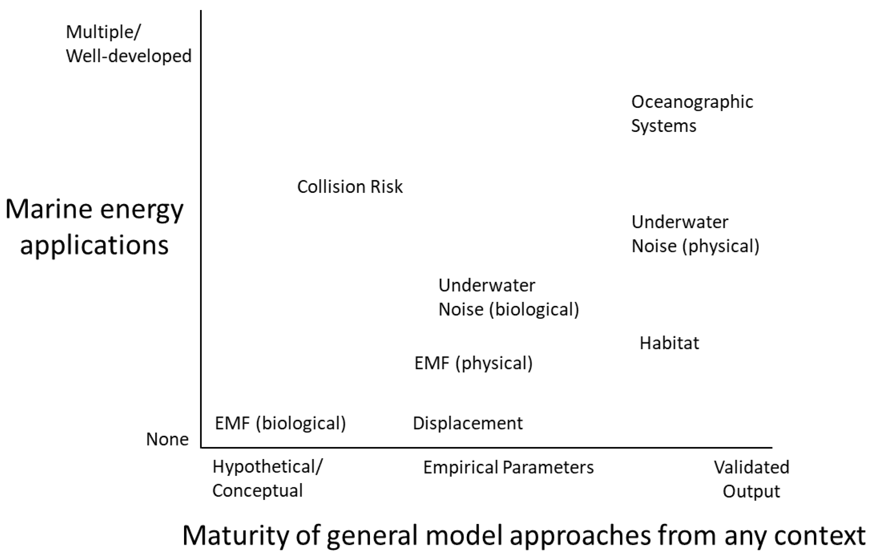
4.1. Availability and Maturity of Models

We have qualitatively sorted the relative availability and maturity of modeling approaches for potential ME stressor-receptor interactions along two axes: the level of development in any context of models that have been or could be used, and the number of published ME model applications (Figure 1). For this purpose, model maturity indicates model refinement (including software availability) and the incorporation of empirical data to parameterize and validate the models in any context. ME applications may be entirely hypothetical or parameterized and validated for specific projects.

The most developed models are for oceanographic systems and underwater noise propagation, which have software models considered reliable for their intended uses. Hydrodynamic, wave, and sediment models have been applied to test sites and hypothetical arrays. Validation of ME applications remains limited [47,48,49,50], but established methods are available once data are collected [30,196,197]. There are fewer ME underwater noise model studies than oceanographic models, but multiple available analytical and software models are applicable [83]. Studies of OSW farm operation demonstrate noise modeling for commercial-scale arrays [96,104]. Behavioral and population models of marine mammals and fish have been applied for pile-driving [81,91,106,115] and generic noise sources [112], but there is a lack of physiological and behavioral response data for ME noise, including the effects of extended exposure.

Models of species-habitat relationships that evaluate habitat stressor-receptor interactions have a robust ecological literature [140,198,199], as do trophic models used to evaluate artificial reefs and exclusion zones and biophysical models used for simulating stepping-stone effects on dispersal [154,200]. Only a few studies have modeled ME effects on habitat [126,144,151], but information, not theory, is the barrier.

Displacement of marine animals avoiding ME installations has received very little attention either in theory or in the field. Avoidance behaviors, however, are not unique, and avoidance of device presence could be added to models of species responses to underwater noise, changes in habitat, or non-ME stressors. As with all behavioral models, the availability of empirical data is a limiting factor.

Two-dimensional models of EMFs generated by submarine cables have been applied in simplified settings. We found no examples of realistic spatial variability (2D or 3D) or interacting fields, and model validation has been rudimentary. Recent improvements in underwater EMF monitoring [137] should facilitate model development. No models of physiological and behavioral responses to underwater EMFs were published at the time of this review, and findings of animal responses to EMFs are inconclusive [127].

Collision risk is a specific field of study with few analogs, and behavioral differences among birds, fish, and marine mammals affect how they should be modeled [182]. Most model studies included swimming and diving characteristics while a few incorporate more detailed behavior [178]. Avoidance or evasion probabilities can be included in most models, but few studies have the necessary data. Comprehensive modeling of collision risk will require research regarding responses to arrays and the effects of sublethal collisions on populations [176].

The coverage of stressor-receptor interactions in modeling studies has been uneven across device types. Tidal turbines, the focus of most reviewed studies, have been modeled for all stressor-receptor interactions except EMF (for which transmission cables have been the focus). WECs have been evaluated for effects on oceanographic systems, and once for underwater noise [97]. We found no models of species responses to WECs.

Only a few of the reviewed studies modeled the effects of large tidal turbine arrays [40,46,49,53,61,63,151] or WEC arrays [66,70] in realistic settings; they involved hypothetical arrays without empirical data and most focused on oceanographic effects. Modeling arrays increases complexity and may require either increasing the spatial scale without corresponding reductions in resolution or adding simplifying assumptions. Arrays introduce interacting wakes and sound waves, dispersal connectivity, and other factors depending on device type and array design. Animals encountering multiple devices may change their behavior further or face additional risks, e.g., reduced ability to evade. In this case, the barrier to understanding is the lack of both theory and information. Significant research and modeling are needed to understand the compounding effects of arrays [3].

4.2. Selecting Modeling Approaches

Progress in project planning and consenting can be accelerated if regulators, researchers, and developers collaborate on modeling frameworks for environmental assessments and monitoring. However, model suites must be chosen for specific projects given the diversity of sites, devices, and receptors. Technical considerations for model selection include the following:

• Device characteristics: Device type, number, and arrangement determine which physical and behavioral processes need to be available in the selected models and what scale and resolution are required.
• Site characteristics: Model functionality needs to be appropriate for the conditions of the site, i.e., water depth, bathymetric complexity, sediment dynamics, and/or biotic interactions.
• Spatiotemporal scales: Computation time is determined by model scale and resolution. It can be improved in some models using simplifications in exchange for specificity. Modeling objectives may require the use of both near- and farfield modeling to estimate both source levels and propagation of effects. The choice of physiological and behavioral functions and parameters may also depend on the scale of the modeling objectives.
• Receptor species: Modeling approaches differ for benthic or pelagic species, mobile or sessile organisms, and different life stages (e.g., adults vs. larvae).
• Existing data: If data of sufficient quality is available to be used in a model analysis, it may constrain the choice of models. This is particularly a consideration if collecting other types of data (in the necessary time frame) is not feasible.

Resources available for modeling must also be considered. Access to existing models and their maturity, the time and budget that can be devoted to modeling, and the expertise needed for development and application all affect model selection. Commercial software has been more readily accepted by developers than research-oriented or customized software [59] and requires less development and setup time. If resources allow, using multiple models and comparing results can increase confidence in model results [52,59].

Using the same model(s) for multiple project types and/or sites reduces the overall effort, enables comparison, and facilitates aggregation of model results for cumulative impact assessments [8]. The transfer of hydrodynamic models and noise depends upon the similarity between sites relative to depth, morphological complexity, and proximity to coastlines. Transferring species models between locations is more straightforward, but non-ME stressors or other site characteristics that affect populations may require changes in mechanisms within the model (i.e., the shape of relationships between environmental factors and species response) or parameters for vital rates or behaviors [201,202,203].

Nearly all reviewed studies focused on a single stressor–receptor interaction (Table A2). Most studies that coupled hydrodynamic models to biological models focused on the biological outcomes, using the hydrodynamic models to provide input data rather than fully exploring the oceanographic effects [106,160,193,204]. Van der Molen et al. [104] applied hydrodynamic/biogeochemical, wave, and acoustic models to evaluate the effects of OSW operation, though only the biogeochemical model included an ecosystem component (plankton and benthos) and the effects were not combined across models. For comprehensive environmental assessments, multipurpose models could increase efficiency, simplify communication, and more effectively estimate cumulative effects, the latter of which is an important component of environmental impact assessments [8]. They can also be used to distinguish between the effects of multiple stressor–receptor interactions on observed population dynamics. For example, agent-based models developed for species responses to noise [81,106,112,117] could be adapted to also include displacement or changes in habitat as drivers of movement and distribution and compare the effects of these behaviors.

4.3. Model Information Requirements and Uncertainties

The broad range of information used in modeling environmental effects of ME, ranging from physical to physiological and behavioral data (

Table 3. Summary of information needs by model type. Not all parameters are needed for all models of a stressor; parameters used less frequently are indicated by parentheses. WSE = water surface elevation; EMF = electromagnetic field; TTS = temporary threshold shift; PTS = permanent threshold shift.

	Device	Morphology/Sediment	Water	Organism Abundance/Distribution	Animal Behavior	Physiology and Vital Rates	Other
Changes in oceanographic systems
Hydrodynamic models	Device geometry or parameters for approximation	Bathymetry, sediment type, and material properties, bottom friction	Current velocity, tides, WSE, temperature, salinity, river discharge				Wind, (precipitation, air temperature)
Wave propagation	Device geometry or parameters for approximation	Bathymetry	WSE, incoming waves, current velocity, tides				Wind, air-sea temperature difference
Underwater noise
Transmission loss	Source sound level	Depth, (material properties of sediment)	Temperature, salinity				(Recorded sound at distance from the source)
Nearfield propagation	Device geometry	Bathymetry, sediment type, and material properties, bottom roughness	WSE, temperature, salinity, surface roughness
Farfield propagation	Source sound level	Bathymetry; sediment type (by layer), roughness, material properties	WSE, temperature, salinity, surface roughness
Species effects	Sound level maps			Species distribution, prey distribution	Swimming, diving, noise response, dispersal, migration	Audiograms, TTS/PTS thresholds, vital rates
EMF
Physical EMF (analytical or numerical)	Cable configuration, burial depth	Sediment type and resistivity	Water resistivity
EMF behavioral response *				Species distribution	Movement, dispersal, behavioral response to EMF	Physiological response to EMF, feeding:growth, vital rates
Changes in habitat
Statistical species distribution		Bathymetry, slope, roughness, sediment type	Current velocity, shear stress, temperature, salinity, chlorophyll, nutrients, dissolved gases	Presence, presence/absence, abundance
Spatial ecosystem and trophic				Abundance, biomass	Dispersal	Feeding, growth, production:biomass, vital rates	Habitat type
Biophysical			Current velocity, (chlorophyll, nutrients, dissolved gases)		Swimming, diving, (foraging, response to devices)	Larval stage duration, larval survival, feeding, growth, production:biomass
Collision risk
Encounter/collision risk	Device geometry	Channel width and depth	Current velocity	Distribution in the water column	Swimming, diving, foraging, avoidance, evasion	Shape, size
Exposure time population model	Device geometry			Distribution in the water column	Diving	Reproduction, survival
Displacement
Biophysical/agent-based			Current velocity, temperature, salinity	Species distribution, prey distribution	Swimming, diving
Statistical species distribution			Current velocity, shear stress, temperature, salinity	Species distribution

), creates challenges when developing and parameterizing models. Those designing monitoring protocols should consider the overlaps in data needs among models and determine whether modeling can reduce or refine monitoring. Existing data and monitoring required by regulation can inform model selection. Coordinating the development of models and monitoring protocols for multiple stressors, or multiple habitats or species of concern, could streamline data collection. For example, bathymetry and water and sediment properties are common needs among physical and habitat models, and many biological models use some combination of swimming, diving, foraging, and/or dispersal behavior. It is important to ensure the correct data are collected at the necessary resolution and extent to be used in all relevant models. Errors in fundamental data, e.g., bathymetry, resulting from inadequate resolution or measurement error can propagate within models and through multiple models, increasing overall uncertainty [28]. Estimation of random error or bias that cannot be corrected can be incorporated into models to understand the effects of uncertainty.

Hydrodynamics and water properties are highly variable and resource-intensive to characterize. Seasonal, interannual, and spatial variability may require extended, site-specific monitoring to accurately inform and validate a model, while also directly assessing effects. Reliable regional ocean models may be adequate substitutes for detailed monitoring data for use as initial conditions, boundary conditions, or forcing factors in oceanographic models. Other physical data, such as bathymetry and seabed properties, are relatively static and may require only one or a few surveys. In some reviewed studies, physical data or regional model outputs were publicly available, but at a spatial resolution that is too coarse [105,126,151]. Lack of data at sufficient resolution is a problem for physical models, especially for habitat, and discrepancies in the resolution of data sources can affect model results [205,206]. The optimal resolutions depend upon site characteristics, including morphological complexity, variability in environmental factors, and the scales of effects and responses relevant to the stressor(s) and receptor(s).

Species distribution data are site-specific and often vary by season and year for both resident species at local scales and migratory species [2]. Data may already be available for well-studied species or locations. Marine mammals and seabirds are more readily observed on the surface than fish or invertebrates, which typically require more intensive sampling methods, but mammal and seabird diving behavior is often poorly understood. Tracking movements and behavior requires acoustic and/or video monitoring systems near devices [207,208] or telemetry at larger scales [209,210,211]. Some studies used prey distribution to model foraging behavior and energetic effects [81,106,117]. When prey distribution was unavailable, authors used baseline distributions of the focal species as a proxy for prey; this requires assuming that prey is not also responding to the ME stressors or otherwise changing over time [212]. The validity of this assumption depends upon the prey species and would require additional monitoring to confirm.

Information about response behavior is scarce because there have been few operating ME devices, observing behavior near them is difficult, and observing behavior around larger arrays has not yet been possible. Recent studies monitoring porpoises and seals near small tidal turbine arrays have experienced limitations such as a lack of data before turbine installation or during multiple seasons and the inability to distinguish between individuals [79,80]. It is yet unknown how much device design and location affect behavior and thus how much species response data can be generalized. Behavioral response data are especially valuable for models of collision risk, displacement, and species effects of noise or EMFs, because of the significant uncertainty involved and the sensitivity of models to these behaviors [182]. Models of hypothesized mechanisms of behavior near devices help refine information needs [178].

Physiological and demographic parameters may be available for species of concern or commercial interest. Most reviewed studies used published data for their receptor species or for similar species rather than collecting new data. Estimating the effects of stressors on health and vital rates has been identified as a significant challenge when using the PCoD approach [115], and the duration and intensity of sampling to detect changes in population dynamics may not be feasible for individual projects. Booth et al. [120] identified metrics that can indicate population-level changes more rapidly than the monitoring required to measure demographic rates or trends in abundance.

In general, environmental and stressor differences, genetic distinctness of populations, and/or differences in food resources should be considered when using data from other locations [202,203]. The age, sex, physical condition, and experience of individuals may affect their physiology and behavior in response to devices, requiring larger sample sizes [213,214,215]. The effects of individual-level variability on population responses, detection probabilities, and the difficulty in estimating age and sex while observing species should be also considered when transferring data or models between sites [216].

4.4. Validation and Feedback between Models and Monitoring

A small proportion of studies in this review, mostly physical models, reported model validation. Studies employed both qualitative (visual) comparisons [49,118,134] and statistical comparisons with empirical data [48,60,86]. In some reviewed studies, results were compared with results from previously validated or more computationally intensive models [47,48,50,87,132]. Visual or otherwise unquantified assessments have been used in oceanographic modeling, but quantitative validation provides objective results, enables model comparison, and allows model accuracy to be tracked when new information is incorporated [25,26,28,30]. Validation of models at one location or for one purpose does not guarantee model accuracy for a new location or application [161].

The lack of data from operating devices, particularly arrays, has been an obstacle for calibrating and validating most stressor-receptor interaction models. In such cases, only baseline (without device) models may be validated [49,52]. Models based on abstract or simplified environments cannot be calibrated or validated with empirical data except perhaps in laboratory settings—an inherent limitation of many research-oriented ME modeling studies. These studies can be used to develop model frameworks, identify data sensitivities, and focus further modeling, but do not by themselves demonstrate the effectiveness or accuracy of the models for environmental assessment.

The information needed for model validation is often the same as that needed for model parameterization, calibration, and initial conditions, e.g., currents and water properties for oceanographic models or species distribution for changes in habitat, displacement, or response to noise/EMFs. Exceptions include physical models of noise and EMFs, many of which do not use measured sound levels or EMFs as inputs but do require them for validating outputs. Species distribution studies have often used all the available observation data to parameterize a model and thus could not validate it with independent data [152,217]. In such cases, cross-validation methods can be used to estimate model accuracy using subsets of the data [164,217,218]. Techniques are also available for validating spatially explicit predictions and observations [164,197].

Discrepancies between model outputs and observations result from a combination of model and observation errors [25,28,30,219]. Monitoring programs that estimate observation errors are important for distinguishing whether discrepancies between model data and observations arise from input or validation data or errors within the model. Accurate input data and model validation are especially important for oceanographic modeling that provides input for other models because the error will propagate from one model to the next [28,161]. Additionally, a biological model that includes only one stressor-receptor interaction may appear to have errors relative to observations because the effects of other stressors on the species are not included. Coordinated models and monitoring of the cumulative effects of multiple stressors can help determine model accuracy and sources of error.

Sensitivity analyses identify parameters or model mechanisms that have the greatest effect on model outcomes but were only included in a small number of reviewed models [52,94,112,118,178,182]. Quantifying uncertainties helps determine the amount, resolution, and quality of data needed from monitoring and research. The value of additional information may differ by location based on local hydrodynamics, bathymetry, prey and competitor species, and so forth, so it is beneficial to conduct a value of information assessment for each project.

5. Conclusions

Modeling capabilities vary broadly across the six ME stressor-receptor interactions in this review, and there is ample room for model improvement for all. For the physical models, the primary needs are the inclusion of realistic spatial complexity and refinement and validation of models with operating devices. Biological models, particularly those including behavioral responses to devices, need further model development and adaptation to inform the research and monitoring necessary for fully functional models. The ability to collect empirical data is much higher for physical than biological components of models and is necessary to improve both. Most ME modeling studies have focused on single stressor-receptor interactions but considering the modeling process holistically can streamline monitoring requirements.

Feedbacks between monitoring and modeling are key for improving environmental assessment for ME devices. Most published studies have modeled abstract systems that cannot be compared with observational data or have been part of a planning process only, without continued use during monitoring of operating devices. Exploratory modeling helps with identifying monitoring needs and refining protocols. Quantitative model validation using observational data remains rare, and for some stressor-receptor interactions may not be possible until more extensive device deployment has occurred. Despite the inherent challenges, validation is vital for improving model performance and increasing developers’ and regulators’ confidence in the models.

We reviewed modeling approaches useful for environmental assessment of the effects of ME development with the intent of strengthening the relationship between modeling and monitoring. While models may not be capable of fully predicting all environmental effects of ME devices in the near term, particularly biological effects, the process of developing and applying models is highly informative for synthesizing information and clarifying research and monitoring needs. Many information gaps identified in this review may be usefully addressed using multi-stressor approaches for research and device testing. A comprehensive approach to stressor-receptor interaction research, monitoring, and modeling can therefore advance the pace of ME development.

References

1. Copping, A.E.; Hemery, L.G. (Eds.) Marine Renewable Energy: Environmental Effects and Monitoring Strategies. In OES-Environmental 2020 State of the Science Report: Environmental Effects of Marine Renewable Energy Development Around the World; Ocean Energy Systems: Seattle, WA, USA, 2020; pp. 18–26. [Google Scholar] [CrossRef]
2. Fox, C.J.; Benjamins, S.; Masden, E.A.; Miller, R. Challenges and opportunities in monitoring the impacts of tidal-stream energy devices on marine vertebrates. Renew. Sustain. Energy Rev. 2018, 81, 1926–1938. [Google Scholar] [CrossRef]
3. Segura, E.; Morales, R.; Somolinos, J.A. A strategic analysis of tidal current energy conversion systems in the European Union. Appl. Energy 2018, 212, 527–551. [Google Scholar] [CrossRef]
4. Boehlert, G.W.; Gill, A.B. Environmental and ecological effects of ocean renewable energy development: A current synthesis. Oceanography 2010, 23, 68–81. [Google Scholar] [CrossRef] [Green Version]
5. Wilding, T.A.; Gill, A.B.; Boon, A.; Sheehan, E.; Dauvin, J.C.; Pezy, J.P.; O’Beirn, F.; Janas, U.; Rostin, L.; De Mesel, I. Turning off the DRIP (‘Data-rich, information-poor’)—Rationalising monitoring with a focus on marine renewable energy developments and the benthos. Renew. Sustain. Energy Rev. 2017, 74, 848–859. [Google Scholar] [CrossRef]
6. Dannheim, J.; Bergström, L.; Birchenough, S.N.R.; Brzana, R.; Boon, A.R.; Coolen, J.W.P.; Dauvin, J.-C.; De Mesel, I.; Derweduwen, J.; Gill, A.B.; et al. Benthic effects of offshore renewables: Identification of knowledge gaps and urgently needed research. ICES J. Mar. Sci. 2019, 77, 1092–1108. [Google Scholar] [CrossRef]
7. Mendoza, E.; Lithgow, D.; Flores, P.; Felix, A.; Simas, T.; Silva, R. A framework to evaluate the environmental impact of OCEAN energy devices. Renew. Sustain. Energy Rev. 2019, 112, 440–449. [Google Scholar] [CrossRef]
8. Willsteed, E.; Gill, A.B.; Birchenough, S.N.R.; Jude, S. Assessing the cumulative environmental effects of marine renewable energy developments: Establishing common ground. Sci. Total Environ. 2017, 577, 19–32. [Google Scholar] [CrossRef] [Green Version]
9. Isaksson, N.; Masden, E.A.; Williamson, B.J.; Costagliola-Ray, M.M.; Slingsby, J.; Houghton, J.D.R.; Wilson, J. Assessing the effects of tidal stream marine renewable energy on seabirds: A conceptual framework. Mar. Pollut. Bull. 2020, 157, 111314. [Google Scholar] [CrossRef]
10. Copping, A.; Gorton, A.; Freeman, M. Data Transferability and Collection Consistency in Marine Renewable Energy; PNNL-27955; U.S. Department of Energy: Richland, WA, USA, 2018.
11. Shen, H.; Zydlewski, G.B.; Viehman, H.A.; Staines, G. Estimating the probability of fish encountering a marine hydrokinetic device. Renew. Energy 2016, 97, 746–756. [Google Scholar] [CrossRef] [Green Version]
12. Cotter, E.; Polagye, B. Automatic Classification of Biological Targets in a Tidal Channel Using a Multibeam Sonar. J. Atmos. Ocean. Technol. 2020, 37, 1437–1455. [Google Scholar] [CrossRef]
13. Isaksson, N.; Cleasby, I.R.; Owen, E.; Williamson, B.J.; Houghton, J.D.R.; Wilson, J.; Masden, E.A. The Use of Animal-Borne Biologging and Telemetry Data to Quantify Spatial Overlap of Wildlife with Marine Renewables. J. Mar. Sci. Eng. 2021, 9, 263. [Google Scholar] [CrossRef]
14. Goh, H.-B.; Lai, S.-H.; Jameel, M.; Teh, H.-M. Potential of coastal headlands for tidal energy extraction and the resulting environmental effects along Negeri Sembilan coastlines: A numerical simulation study. Energy 2020, 192, 116656. [Google Scholar] [CrossRef]
15. Shabtay, A.; Portman, M.E.; Ofir, E.; Carmel, Y.; Gal, G. Using ecological modelling in marine spatial planning to enhance ecosystem-based management. Mar. Policy 2018, 95, 14–23. [Google Scholar] [CrossRef]
16. Ehler, C.; Douvere, F. Marine spatial planning: A step-by-step approach toward ecosystem-based management. In Intergovernmental Oceanographic Commission and Man and the Biosphere Programme; IOC Manual and Guides No. 53, ICAM Dossier No. 6; UNESCO: Paris, France, 2009. [Google Scholar]
17. Bender, A.; Francisco, F.; Sundberg, J. A Review of Methods and Models for Environmental Monitoring of Marine Renewable Energy. In Proceedings of the 12th European Wave and Tidal Energy Conference, Cork, Ireland, 27 August–1 September 2017. [Google Scholar]
18. Ozkan, C.; Perez, K.; Mayo, T. The impacts of wave energy conversion on coastal morphodynamics. Sci. Total Environ. 2020, 712, 136424. [Google Scholar] [CrossRef]
19. Laín, S.; Contreras, L.T.; López, O. A review on computational fluid dynamics modeling and simulation of horizontal axis hydrokinetic turbines. J. Braz. Soc. Mech. Sci. Eng. 2019, 41, 375. [Google Scholar] [CrossRef]
20. Nachtane, M.; Tarfaoui, M.; Goda, I.; Rouway, M. A review on the technologies, design considerations and numerical models of tidal current turbines. Renew. Energy 2020, 157, 1274–1288. [Google Scholar] [CrossRef]
21. Copping, A.; Battey, H.; Brown-Saracino, J.; Massaua, M.; Smith, C. An international assessment of the environmental effects of marine energy development. Ocean Coast. Manag. 2014, 99, 3–13. [Google Scholar] [CrossRef]
22. Buenau, K.E.; Garavelli, L.J.; Hemery, L.G.; Garcia Medina, G.; Hibler, L.F. Review of Available Models for Environmental Effects of Marine Renewable Energy; PNNL-29977; Pacific Northwest National Laboratory: Richland, WA, USA, 2020.
23. Copping, A.; Sather, N.; Hanna, L.; Whiting, J.; Zydlewski, G.; Staines, G.; Gill, A.; Hutchison, I.; O’Hagan, A.; Simas, T.; et al. Annex IV 2016 State of the Science Report: Environmental Effects of Marine Renewable Energy Development around the World. Report for Ocean Energy Systems (OES); Ocean Energy Systems: Seattle, WA, USA, 2016; pp. 1–199.
24. Whiting, J.; Copping, A.; Freeman, M.; Woodbury, A. Tethys knowledge management system: Working to advance the marine renewable energy industry. Int. Mar. Energy J. 2019, 2, 29–38. [Google Scholar] [CrossRef]
25. Hipsey, M.R.; Gal, G.; Arhonditsis, G.B.; Carey, C.C.; Elliott, J.A.; Frassl, M.A.; Janse, J.H.; de Mora, L.; Robson, B.J. A system of metrics for the assessment and improvement of aquatic ecosystem models. Environ. Model. Softw. 2020, 128, 04697. [Google Scholar] [CrossRef]
26. Kubicek, A.; Jopp, F.; Breckling, B.; Lange, C.; Reuter, H. Context-oriented model validation of individual-based models in ecology: A hierarchically structured approach to validate qualitative, compositional and quantitative characteristics. Ecol. Complex. 2015, 22, 178–191. [Google Scholar] [CrossRef]
27. Bennett, N.D.; Croke, B.F.W.; Guariso, G.; Guillaume, J.H.A.; Hamilton, S.H.; Jakeman, A.J.; Marsili-Libelli, S.; Newham, L.T.H.; Norton, J.P.; Perrin, C.; et al. Characterising performance of environmental models. Environ. Model. Softw. 2013, 40, 1–20. [Google Scholar] [CrossRef]
28. Williams, J.J.; Esteves, L.S. Guidance on Setup, Calibration, and Validation of Hydrodynamic, Wave, and Sediment Models for Shelf Seas and Estuaries. Adv. Civ. Eng. 2017, 2017, 5251902. [Google Scholar] [CrossRef]
29. Gregr, E.J.; Palacios, D.M.; Thompson, A.; Chan, K.M.A. Why less complexity produces better forecasts: An independent data evaluation of kelp habitat models. Ecography 2019, 42, 428–443. [Google Scholar] [CrossRef]
30. Stow, C.A.; Jolliff, J.; McGillicuddy, D.J.; Doney, S.C.; Allen, J.I.; Friedrichs, M.A.M.; Rose, K.A.; Wallhead, P. Skill assessment for coupled biological/physical models of marine systems. J. Mar. Syst. 2009, 76, 4–15. [Google Scholar] [CrossRef] [Green Version]
31. De Dominicis, M.; O’Hara Murray, R.; Wolf, J. Multi-scale ocean response to a large tidal stream turbine array. Renew. Energy 2017, 114, 1160–1179. [Google Scholar] [CrossRef]
32. Haas, K.; Yang, X.; Fritz, H. Modeling impacts of energy extraction from the Gulf Stream system. In Proceedings of the 2nd Annual Marine Energy Technology Symposium (METS), Seattle, WA, USA, 15–17 April 2014. [Google Scholar]
33. Bergillos, R.J.; Rodriguez-Delgado, C.; Iglesias, G. Wave farm impacts on coastal flooding under sea-level rise: A case study in southern Spain. Sci. Total Environ. 2019, 653, 1522–1531. [Google Scholar] [CrossRef] [PubMed]
34. Pacheco, A.; Gorbeña, E.; Plomaritis, T.A.; Garel, E.; Gonçalves, J.M.S.; Bentes, L.; Monteiro, P.; Afonso, C.M.L.; Oliveira, F.; Soares, C.; et al. Deployment characterization of a floatable tidal energy converter on a tidal channel, Ria Formosa, Portugal. Energy 2018, 158, 89–104. [Google Scholar] [CrossRef] [Green Version]
35. Hill, C.; Neary, V.S.; Guala, M.; Sotiropoulos, F. Performance and Wake Characterization of a Model Hydrokinetic Turbine: The Reference Model 1 (RM1) Dual Rotor Tidal Energy Converter. Energies 2020, 13, 5145. [Google Scholar] [CrossRef]
36. Bergillos, R.J.; López-Ruiz, A.; Medina-López, E.; Moñino, A.; Ortega-Sánchez, M. The role of wave energy converter farms on coastal protection in eroding deltas, Guadalfeo, southern Spain. J. Clean. Prod. 2018, 12, 356–367. [Google Scholar] [CrossRef]
37. Salunkhe, S.; El Fajri, O.; Bhushan, S.; Thompson, D.; O’Doherty, D.; O’Doherty, T.; Mason-Jones, A. Validation of Tidal Stream Turbine Wake Predictions and Analysis of Wake Recovery Mechanism. J. Mar. Sci. Eng. 2019, 7, 362. [Google Scholar] [CrossRef] [Green Version]
38. Li, X.; Li, M.L.; Jordanm, L.-B.; McLelland, S.; Parsons, D.R.; Amoudry, L.O.; Song, Q.; Comerford, L. Modelling impacts of tidal stream turbines on surface waves. Renew. Energy 2019, 10, 725–734. [Google Scholar] [CrossRef]
39. Soto-Rivas, K.; Richter, D.; Escauriaza, C. A formulation of the thrust coefficient for representing finite-sized farms of tidal energy converters. Energies 2019, 12, 3861. [Google Scholar] [CrossRef] [Green Version]
40. Thiebot, J.; Guillou, N.; Guillou, S.; Good, A.; Lewis, M. Wake field study of tidal turbines under realistic flow conditions. Renew. Energy 2020, 151, 1196–1208. [Google Scholar] [CrossRef]
41. Ahmed, U.; Apsley, D.D.; Afgan, I.; Stallard, T.; Stansby, P.K. Fluctuating loads on a tidal turbine due to velocity shear and turbulence: Comparison of CFD with field data. Renew. Energy 2017, 112, 235–246. [Google Scholar] [CrossRef] [Green Version]
42. Lloyd, T.P.; Turnock, S.R.; Humphrey, V.F. Assessing the influence of inflow turbulence on noise and performance of a tidal turbine using large eddy simulations. Renew. Energy 2014, 71, 742–754. [Google Scholar] [CrossRef]
43. Sufian, S.F.; Li, M.; O’Connor, B.A. 3D modelling of impacts from waves on tidal turbine wake characteristics and energy output. Renew. Energy 2017, 114, 308–322. [Google Scholar] [CrossRef] [Green Version]
44. Churchfield, M.J.; Li, Y.; Moriarty, P.J. A large-eddy simulation study of wake propagation and power production in an array of tidal-current turbines. Philos. Trans. R. Soc. A 2013, 371, 20120421. [Google Scholar] [CrossRef] [PubMed] [Green Version]
45. Adcock, T.A.; Draper, S.; Nishino, T. Tidal power generation—A review of hydrodynamic modelling. Proc. Inst. Mech. Eng. Part A J. Power Energy 2015, 229, 755–771. [Google Scholar] [CrossRef]
46. Thiébot, J.; Guillou, S.; Nguyen, V.T. Modelling the effect of large arrays of tidal turbines with depth-averaged Actuator Disks. Ocean Eng. 2016, 126, 265–275. [Google Scholar] [CrossRef]
47. Sjökvist, L.; Göteman, M.; Rahm, M.; Waters, R.; Svensson, O.; Strömstedt, E.; Leijon, M. Calculating buoy response for a wave energy converter—A comparison of two computational methods and experimental results. Theor. Appl. Mech. Lett. 2017, 7, 164–168. [Google Scholar] [CrossRef]
48. Xu, C.; Huang, Z. Three-dimensional CFD simulation of a circular OWC with a nonlinear power-takeoff: Model validation and a discussion on resonant sloshing inside the pneumatic chamber. Ocean Eng. 2019, 176, 184–198. [Google Scholar] [CrossRef]
49. Ashall, L.M.; Mulligan, R.P.; Law, B.A. Variability in suspended sediment concentration in the Minas Basin, Bay of Fundy, and implications for changes due to tidal power extraction. Coast. Eng. 2016, 107, 102–115. [Google Scholar] [CrossRef]
50. Yang, Z.; Wang, T.; Copping, A.E. Modeling tidal stream energy extraction and its effects on transport processes in a tidal channel and bay system using a three-dimensional coastal ocean model. Renew. Energy 2013, 50, 605–613. [Google Scholar] [CrossRef]
51. Ahmadian, R.; Falconer, R.; Bockelmann-Evans, B. Far-field modelling of the hydro-environmental impact of tidal stream turbines. Renew. Energy 2012, 38, 107–116. [Google Scholar] [CrossRef]
52. Waldman, S.; Bastón, S.; Nemalidinne, R.; Chatzirodou, A.; Venugopal, V.; Side, J. Implementation of tidal turbines in MIKE 3 and Delft3D models of Pentland Firth & Orkney Waters. Ocean Coast. Manag. 2017, 147, 21–36. [Google Scholar] [CrossRef] [Green Version]
53. Chatzirodou, A.; Karunarathna, H.; Reeve, D.E. 3D modelling of the impacts of in-stream horizontal-axis Tidal Energy Converters (TECs) on offshore sandbank dynamics. Appl. Ocean Res. 2019, 21, 101882. [Google Scholar] [CrossRef]
54. Chen, C.; Liu, H.; Beardsley, R.C. An unstructured grid, finite-volume, three-dimensional, primitive equations ocean model: Application to coastal ocean and estuaries. J. Atmos. Ocean. Technol. 2003, 20, 159–186. [Google Scholar] [CrossRef]
55. Deltares. Simulation of Multi-Dimensional Hydrodynamic Flows and Transport Phenomena, Including Sediments, User Manual, Version 3.15; Deltares: Delft, The Netherlands, 2021; p. 702. [Google Scholar]
56. DHI. Mike 3 Flow Model, Hydrodynamic Module, User Guide; DHI: Hørsholm, Denmark, 2017; p. 128. [Google Scholar]
57. Hervouet, J.-M. TELEMAC modelling system: An overview. Hydrol. Processes 2000, 14, 2209–2210. [Google Scholar] [CrossRef]
58. Piggott, M.; Gorman, G.; Pain, C.; Allison, P.; Candy, A.; Martin, B.; Wells, M. A new computational framework for multi-scale ocean modelling based on adapting unstructured meshes. Int. J. Numer. Methods Fluids 2008, 56, 1003–1015. [Google Scholar] [CrossRef]
59. Gallego, J.; Side, J.; Baston, S.; Waldman, S.; Bell, M.; James, M.; Davies, I.; O’ Hara Murray, R.; Heath, M.; Sabatino, A.; et al. Large scale three-dimensional modeling for wave and tidal energy resource and environmental impact; Methodologies for quantifying acceptable thresholds for sustainable exploitation. Ocean Coast. Manag. 2017, 147, 67–77. [Google Scholar] [CrossRef] [Green Version]
60. Jones, C.; Chang, G.; Raghukumar, K.; McWilliams, S. Spatial Environmental Assessment Tool (SEAT): A modeling tool to evaluate potential environmental risks associated with wave energy converter deployments. Energies 2018, 11, 2036. [Google Scholar] [CrossRef] [Green Version]
61. Robins, P.E.; Neill, S.P.; Lewis, M.J. Impact of tidal-stream arrays in relation to the natural variability of sedimentary processes. Renew. Energy 2014, 72, 311–321. [Google Scholar] [CrossRef] [Green Version]
62. Haverson, D.; Bacon, J.; Smith, H.C.M.; Venugopal, V. Modelling the hydrodynamic and morphological impacts of a tidal stream development in Ramsey Sound. Renew. Energy 2018, 22, 876–887. [Google Scholar] [CrossRef]
63. Martin-Short, R.; Hill, J.; Kramer, S.C.; Avdis, A.; Allison, P.A.; Piggott, M.D. Tidal resource extraction in the Pentland Firth, UK: Potential impacts on flow regime and sediment transport in the Inner Sound of Stroma. Renew. Energy 2015, 76, 596–607. [Google Scholar] [CrossRef] [Green Version]
64. Beels, C.; Troch, P.; De Backer, G.; Vantorre, M.; De Rouck, J. Numerical implementation and sensitivity analysis of a wave energy converter in a time-dependent mild-slope equation model. Coast. Eng. 2010, 57, 471–492. [Google Scholar] [CrossRef]
65. Stratigaki, V.; Troch, P.; Forehand, D. A fundamental coupling methodology for modeling near-field and far-field wave effects of floating structures and wave energy devices. Renew. Energy 2019, 143, 1608–1627. [Google Scholar] [CrossRef]
66. Venugopal, V.; Nemalidinne, R.; Vögler, A. Numerical modelling of wave energy resources and assessment of wave energy extraction by large scale wave farms. Ocean Coast. Manag. 2017, 147, 37–48. [Google Scholar] [CrossRef]
67. Penalba, M.; Kelly, T.; Ringwood, J. Using NEMOH for Modelling Wave Energy Converters: A Comparative Study with WAMIT. In Proceedings of the 12th European Wave and Tidal Energy Conference (EWTEC), Cork, Ireland, 1 September 2017. [Google Scholar]
68. Verao Fernandez, G.; Stratigaki, V.; Troch, P. Irregular Wave Validation of a Coupling Methodology for Numerical Modelling of Near and Far Field Effects of Wave Energy Converter Arrays. Energies 2019, 12, 538. [Google Scholar] [CrossRef] [Green Version]
69. Abanades, J.; Greaves, D.; Iglesias, G. Wave farm impact on the beach profile: A case study. Coast. Eng. 2014, 86, 36–44. [Google Scholar] [CrossRef]
70. O’Dea, A.; Haller, M.C.; Özkan-Haller, H.T. The impact of wave energy converter arrays on wave-induced forcing in the surf zone. Ocean Eng. 2018, 161, 322–336. [Google Scholar] [CrossRef]
71. Balitsky, P.; Quartier, N.; Stratigaki, V.; Verao Fernandez, G.; Vasarmidis, P.; Troch, P. Analysing the near-field effects and the power production of near-shore WEC array using a new wave-to-wire model. Water 2019, 11, 1137. [Google Scholar] [CrossRef] [Green Version]
72. Babarit, A.; Delhommeau, G. Theoretical and numerical aspects of the open source BEM solver {NEMOH}. In Proceedings of the 11th EuropeanWave and Tidal Energy Conference, Nantes, France, 6–11 September 2015. [Google Scholar]
73. Guillou, N.; Lavidas, G.; Chapalain, G. Wave Energy Resource Assessment for Exploitation—A Review. J. Mar. Sci. Eng. 2020, 8, 705. [Google Scholar] [CrossRef]
74. Cavaleri, L.; Abdalla, S.; Benetazzo, A.; Bertotti, L.; Bidlot, J.R.; Breivik, Ø.; Carniel, S.; Jensen, R.E.; Portilla-Yandun, J.; Rogers, W.E.; et al. Wave modelling in coastal and inner seas. Prog. Oceanogr. 2018, 167, 164–233. [Google Scholar] [CrossRef]
75. Kang, S.; Borazjani, I.; Colby, J.A.; Sotiropoulos, F. Numerical simulation of 3D flow past a real-life marine hydrokinetic turbine. Adv. Water Resour. 2012, 39, 33–43. [Google Scholar] [CrossRef]
76. Contardo, S.; Hoeke, R.; Hemer, M.; Symonds, G.; McInnes, K.; O’Grady, J. In situ observations and simulations of coastal wave field transformation by wave energy converters. Coast. Eng. 2018, 140, 175–188. [Google Scholar] [CrossRef]
77. Popper, A.N.; Hawkins, A. (Eds.) The Effects of Noise on Aquatic Life II; Springer: New York, NY, USA, 2016. [Google Scholar] [CrossRef]
78. Hastie, G.D.; Russell, D.J.F.; McConnell, B.; Moss, S.; Thompson, D.; Janik, V.M. Sound exposure in harbour seals during the installation of an offshore wind farm: Predictions of auditory damage. J. Appl. Ecol. 2015, 52, 631–640. [Google Scholar] [CrossRef] [Green Version]
79. Palmer, L.; Gillespie, D.; MacAulay, J.D.J.; Sparling, C.E.; Russell, D.J.F.; Hastie, G.D. Harbour porpoise (Phocoena phocoena) presence is reduced during tidal turbine operation. Aquat. Conserv. Mar. Freshw. Ecosyst. 2021, 31, 3543–3553. [Google Scholar] [CrossRef]
80. Onoufriou, J.; Russell, D.J.F.; Thompson, D.; Moss, S.E.; Hastie, G.D. Quantifying the effects of tidal turbine array operations on the distribution of marine mammals: Implications for collision risk. Renew. Energy 2021, 180, 157–165. [Google Scholar] [CrossRef]
81. Nabe-Nielsen, J.; Sibly, R.M.; Tougaard, J.; Teilmann, J.; Sveegaard, S. Effects of noise and by-catch on a Danish harbour porpoise population. Ecol. Model. 2014, 272, 242–251. [Google Scholar] [CrossRef] [Green Version]
82. Pine, M.K.; Schmitt, P.; Culloch, R.M.; Lieber, L.; Kregting, L.T. Providing ecological context to anthropogenic subsea noise: Assessing listening space reductions of marine mammals from tidal energy devices. Renew. Sustain. Energy Rev. 2019, 103, 49–57. [Google Scholar] [CrossRef] [Green Version]
83. Etter, P.C. Underwater Acoustic Modeling and Simulation, 5th ed.; CRC Press: Boca Raton, FL, USA, 2018. [Google Scholar]
84. Urick, R. Principles of Underwater Sound, 3rd ed.; Peninsula Publishing: Westport, CT, USA, 1983. [Google Scholar]
85. Bailey, H.; Senior, B.; Simmons, D.; Rusin, J.; Picken, G.; Thompson, P.M. Assessing underwater noise levels during pile-driving at an offshore windfarm and its potential effects on marine mammals. Mar. Pollut. Bull. 2010, 60, 888–897. [Google Scholar] [CrossRef] [PubMed]
86. Pine, M.K.; Jeffs, A.G.; Radford, C.A. The cumulative effect on sound levels from multiple underwater anthropogenic sound sources in shallow coastal waters. J. Appl. Ecol. 2014, 51, 23–30. [Google Scholar] [CrossRef] [Green Version]
87. Lippert, T.; Ainslie, M.A.; von Estorff, O. Pile driving acoustics made simple: Damped cylindrical spreading model. J. Acoust. Soc. Am. 2018, 143, 310–317. [Google Scholar] [CrossRef] [PubMed]
88. Zampolli, M.; Nijhof, M.J.J.; Jong, C.A.F.d.; Ainslie, M.A.; Jansen, E.H.W.; Quesson, B.A.J. Validation of finite element computations for the quantitative prediction of underwater noise from impact pile driving. J. Acoust. Soc. Am. 2013, 133, 72–81. [Google Scholar] [CrossRef]
89. Robertson, F.; Wood, J.; Joslin, J.; Joy, R.; Polagye, B. Marine Mammal Behavioral Response to Tidal Turbine Sound, Final Technical Report for DE-EE0006385; University of Washington: Seattle, WA, USA, 2018. [Google Scholar]
90. Talisman. Beatrice Wind Farm Demonstrator Project: Environmental Statement; D/2875/2005; Talisman Energy (UK) Limited: Aberdeen, Scotland, 2005. [Google Scholar]
91. Middel, H.; Verones, F. Making marine noise pollution impacts heard: The case of cetaceans in the North Sea within life cycle impact assessment. Sustainability 2017, 9, 1138. [Google Scholar] [CrossRef] [Green Version]
92. Ainslie, M.A.; Halvorsen, M.B.; Muller, R.A.J.; Lippert, T. Application of damped cylindrical spreading to assess range to injury threshold for fishes from impact pile driving. J. Acoust. Soc. Am. 2020, 148, 108–121. [Google Scholar] [CrossRef]
93. Richardson, W.; Thomson, D. Marine Mammals and Noise; Gulf Professional Publishing: Ontario, QC, Canada, 1995. [Google Scholar]
94. Lippert, T.; von Estorff, O. The significance of parameter uncertainties for the prediction of offshore pile driving noise. J. Acoust. Soc. Am. 2014, 136, 2463–2471. [Google Scholar] [CrossRef]
95. Farcas, A.; Thompson, P.M.; Merchant, N.D. Underwater noise modelling for environmental impact assessment. Environ. Impact Assess. Rev. 2016, 57, 114–122. [Google Scholar] [CrossRef] [Green Version]
96. Marmo, B.; Roberts, I.; Buckingham, M.P.; King, S.; Booth, C. Modelling of Noise Effects of Operational Offshore Wind Turbines Including Noise Transmission through Various Foundation Types; Scottish Government: Edinburgh, UK, 2013.
97. Ikpekha, O.; Soberón, F.; Daniels, S. Modelling the propagation of underwater acoustic signals of a marine energy device using finite element method. Renew. Energy Power Qual. J. 2014, 12, 97–102. [Google Scholar] [CrossRef]
98. Kim, H.; Miller, J.; Potty, G. Predicting underwater radiated noise levels due to the first offshore wind turbine installation in the United States. J. Acoust. Soc. Am. 2013, 133, 3419. [Google Scholar] [CrossRef]
99. Hafla, E.; Johnson, E.; Johnson, C.N.; Preston, L.; Aldridge, D.; Roberts, J.D. Modeling underwater noise propagation from marine hydrokinetic power devices through a time-domain, velocity-pressure solution. J. Acoust. Soc. Am. 2018, 143, 3242–3253. [Google Scholar] [CrossRef] [PubMed]
100. Etter, P.C. Review of ocean-acoustic models. In Proceedings of the OCEANS, Biloxi, MS, USA, 26–29 October 2009; pp. 1–6. [Google Scholar]
101. Jensen, F.; Kuperman, W.; Porter, M.; Schmidt, H. Computational Ocean Acoustics, 2nd ed.; Springer: New York, NY, USA, 2011. [Google Scholar] [CrossRef] [Green Version]
102. Lloyd, T.; Humphrey, V.; Turnock, S. Noise modelling of tidal turbine arrays for environmental impact assessment. In Proceedings of the 9th European Wave and Tidal Energy Conference, Southampton, UK, 5–9 September 2011. [Google Scholar]
103. Maggi, A.; Duncan, A. AcTUP v 2.2l Acoustic Toolbox; Center for Marine Science and Technology, Curtin University of Technology: Perth, Australia, 2005. [Google Scholar]
104. van der Molen, J.; Smith, H.C.M.; Lepper, P.; Limpenny, S.; Rees, J. Predicting the large-scale consequences of offshore wind turbine array development on a North Sea ecosystem. Cont. Shelf Res. 2014, 85, 60–72. [Google Scholar] [CrossRef] [Green Version]
105. Lin, Y.-T.; Newhall, A.E.; Miller, J.H.; Potty, G.R.; Vigness-Raposa, K.J. A three-dimensional underwater sound propagation model for offshore wind farm noise prediction. J. Acoust. Soc. Am. 2019, 145, EL335–EL340. [Google Scholar] [CrossRef]
106. Rossington, K.; Benson, T.; Lepper, P.; Jones, D. Eco-hydro-acoustic modeling and its use as an EIA tool. Mar. Pollut. Bull. 2013, 75, 235–243. [Google Scholar] [CrossRef]
107. Whyte, K.F.; Russell, D.J.F.; Sparling, C.E.; Binnerts, B.; Hastie, G.D. Estimating the effects of pile driving sounds on seals: Pitfalls and possibilities. J. Acoust. Soc. Am. 2020, 147, 3948–3958. [Google Scholar] [CrossRef]
108. Tetra Tech. Underwater Acoustic Modeling Report: Virginia Offshore Wind Technology Advancement Project (VOWTAP); Tetra Tech: Glen Allen, VA, USA, 2013. [Google Scholar]
109. Southall, B.; Bowles, A.; Ellison, W.; Finneran, J.; Gentry, R.; Greene, C.J.; Kastak, D.; Ketten, D.; Miller, J.; Nachtigall, P.; et al. Marine mammal noise exposure criteria: Initial scientific recommendations. Aquat. Mamm. 2007, 33, 411–521. [Google Scholar] [CrossRef]
110. Southall, B.L.; Finneran, J.J.; Rcichmuth, C.; Nachtigall, P.E.; Ketten, D.R.; Bowles, A.E.; Ellison, W.T.; Nowacek, D.P.; Tyack, P.L. Marine mammal noise exposure criteria: Updated scientific recommendations for residual hearing effects. Aquat. Mamm. 2019, 45, 125–232. [Google Scholar] [CrossRef]
111. Nedelec, S.L.; Campbell, J.; Radford, A.N.; Simpson, S.D.; Merchant, N.D. Particle motion: The missing link in underwater acoustic ecology. Methods Ecol. Evol. 2016, 7, 836–842. [Google Scholar] [CrossRef] [Green Version]
112. Donovan, C.R.; Harris, C.M.; Milazzo, L.; Harwood, J.; Marshall, L.; Williams, R. A simulation approach to assessing environmental risk of sound exposure to marine mammals. Ecol. Evol. 2017, 7, 2101–2111. [Google Scholar] [CrossRef] [Green Version]
113. New, L.F.; Clark, J.S.; Costa, D.P.; Fleishman, E.; Hindell, M.A.; Klanjšček, T.; Lusseau, D.; Kraus, S.; McMahon, C.R.; Robinson, P.W.; et al. Using short-term measures of behaviour to estimate long-term fitness of southern elephant seals. Mar. Ecol. Prog. Ser. 2014, 496, 99–108. [Google Scholar] [CrossRef] [Green Version]
114. Harwood, J.; King, S.; Schick, R.S.; Donovan, C.R.; Booth, C. A protocol for implementing the Interim Population Consequences of Disturbance (PCoD) approach: Quantifying and assessing the effects of UK offshore renewable energy developments on marine mammal populations. Scott. Mar. Freshw. Sci. 2014, 5, 97. [Google Scholar]
115. Pirotta, E.; Booth, C.G.; Costa, D.P.; Fleishman, E.; Kraus, S.D.; Lusseau, D.; Moretti, D.; New, L.F.; Schick, R.S.; Schwarz, L.K.; et al. Understanding the population consequences of disturbance. Ecol. Evol. 2018, 8, 9934–9946. [Google Scholar] [CrossRef]
116. King, S.L.; Schick, R.S.; Donovan, C.; Booth, C.G.; Burgman, M.; Thomas, L.; Harwood, J. An interim framework for assessing the population consequences of disturbance. Methods Ecol. Evol. 2015, 6, 1150–1158. [Google Scholar] [CrossRef]
117. Nabe-Nielsen, J.; van Beest, F.M.; Grimm, V.; Sibly, R.M.; Teilmann, J.; Thompson, P.M. Predicting the impacts of anthropogenic disturbances on marine populations. Conserv. Lett. 2018, 11, e12563. [Google Scholar] [CrossRef] [Green Version]
118. Thompson, P.M.; Hastie, G.D.; Nedwell, J.; Barham, R.; Brookes, K.L.; Cordes, L.S.; Bailey, H.; McLean, N. Framework for assessing impacts of pile-driving noise from offshore wind farm construction on a harbour seal population. Environ. Impact Assess. Rev. 2013, 43, 73–85. [Google Scholar] [CrossRef] [Green Version]
119. Harwood, J.; Booth, C.; Sinclair, R.R.; Hague, E. Developing marine mammal Dynamic Energy Budget models and their potential for integration into the iPCoD framework. Scott. Mar. Freshw. Sci. 2020, 11, 74. [Google Scholar] [CrossRef]
120. Booth, C.G.; Sinclair, R.R.; Harwood, J. Methods for monitoring for the population consequences of disturbance in marine mammals: A review. Front. Mar. Sci. 2020, 7, 115. [Google Scholar] [CrossRef] [Green Version]
121. Risch, D.; van Geel, N.; Gillespie, D.; Wilson, B. Characterisation of underwater operational sound of a tidal stream turbine. J. Acoust. Soc. Am. 2020, 147, 2547–2555. [Google Scholar] [CrossRef] [Green Version]
122. Schmitt, P.; Pine, M.K.; Culloch, R.M.; Lieber, L.; Kregting, L.T. Noise characterization of a subsea tidal kite. J. Acoust. Soc. Am. 2018, 144, El441. [Google Scholar] [CrossRef]
123. Buscaino, G.; Mattiazzo, G.; Sannino, G.; Papale, E.; Bracco, G.; Grammauta, R.; Carillo, A.; Kenny, J.M.; De Cristofaro, N.; Ceraulo, M.; et al. Acoustic impact of a wave energy converter in Mediterranean shallow waters. Sci. Rep. 2019, 9, 9586. [Google Scholar] [CrossRef] [PubMed] [Green Version]
124. Lippert, S.; Nijhof, M.; Lippert, T.; Wilkes, D.; Gavrilov, A.; Heitmann, K.; Ruhnau, M.; Estorff, O.v.; Schäfke, A.; Schäfer, I.; et al. COMPILE—A generic benchmark case for predictions of marine pile-driving noise. IEEE J. Ocean. Eng. 2016, 41, 1061–1071. [Google Scholar] [CrossRef]
125. van Beest, F.M.; Nabe-Nielsen, J.; Carstensen, J.; Teilmann, J.; Tougaard, J. Disturbance Effects on the Harbour Porpoise Population in the North Sea (DEPONS): Status Report on Model Development; Aarhus University, DCE—Danish Centre for Environment and Energy: Aarhus, Denmark, 2015; p. 43. [Google Scholar]
126. Alexander, K.A.; Meyjes, S.A.; Heymans, J.J. Spatial ecosystem modelling of marine renewable energy installations: Gauging the utility of Ecospace. Ecol. Model. 2016, 331, 115–128. [Google Scholar] [CrossRef]
127. Albert, L.; Deschamps, F.; Jolivet, A.; Olivier, F.; Chauvaud, L.; Chauvaud, S. A current synthesis on the effects of electric and magnetic fields emitted by submarine power cables on invertebrates. Mar. Environ. Res. 2020, 159, 104958. [Google Scholar] [CrossRef] [PubMed]
128. Lee, W.; Yang, K.-L. Using medaka embryos as a model system to study biological effects of the electromagnetic fields on development and behavior. Ecotoxicol. Environ. Saf. 2014, 108, 187–194. [Google Scholar] [CrossRef] [PubMed]
129. Scott, K.; Harsanyi, P.; Lyndon, A.R. Understanding the effects of electromagnetic field emissions from Marine Renewable Energy Devices (MREDs) on the commercially important edible crab, Cancer pagurus (L.). Front. Mar. Sci. 2018, 131, 580–588. [Google Scholar] [CrossRef]
130. Gill, A.; Gloyne-Philips, I.; Kimber, J.; Sigray, P. Marine renewable energy, electromagnetic (EM) fields and EM-sensitive animals. In Marine Renewable Energy Technology and Environmental Interactions; Shields, M., Payne, A., Eds.; Springer: Dordrecht, The Netherlands, 2014. [Google Scholar]
131. Slater, M.; Schultz, A.; Jones, R.; Fischer, C. Electromagnetic Field Study; Oregon Wave Energy Trust: Portland, OR, USA, 2010; 346p.
132. Lucca, G. Analytical evaluation of sub-sea ELF electromagnetic field generated by submarine power cables. Prog. Electromagn. Res. B 2013, 56, 309–326. [Google Scholar] [CrossRef] [Green Version]
133. Huang, Y.; Gloyne-Philips, I. Electromagnetic Simulation of 135 kV Three-Phase Submarine Power Cables; CMACS (Centre for Marine and Coastal Studies Ltd.): Liverpool, England, 2005.
134. Dhanak, M.; Coulson, R.; Dibiasio, C.; Frankenfield, J.; Henderson, E.; Pugsley, D.; Valdes, G. Assessment of electromagnetic field emissions from subsea cables. In Proceedings of the 4th Marine Energy Technology Symposium (METS), Washington, DC, USA, 25–27 April 2016. [Google Scholar]
135. Kavet, R.; Wyman, M.T.; Klimley, A.P. Modeling magnetic fields from a DC power cable buried beneath San Francisco Bay based on empirical measurements. PLoS ONE 2016, 11, e0148543. [Google Scholar] [CrossRef] [PubMed] [Green Version]
136. Gill, A.B.; Huang, Y.; Spencer, J.; Gloyne-Philips, I. Electromagnetic fields emitted by high voltage alternating current offshore wind power cables and interactions with marine organisms. In Proceedings of the Electromagnetics in Current and Emerging Energy Power Systems Seminar, London, UK, 17–23 June 2013. [Google Scholar]
137. Hutchison, Z.L.; Gill, A.B.; Sigray, P.; He, H.; King, J.W. Anthropogenic electromagnetic fields (EMF) influence the behaviour of bottom-dwelling marine species. Sci. Rep. 2020, 10, 4219. [Google Scholar] [CrossRef] [Green Version]
138. Dhanak, M.; An, E.; Coulson, R.; Frankenfield, J.; Ravenna, S.; Pugsley, D.; Valdes, G.; Venezia, W. AUV-based characterization of EMF emissions from submerged power cables. In Proceedings of the OCEANS 2015, Genova, Italy, 18–21 May 2015; pp. 1–6. [Google Scholar]
139. Thomsen, F.; Gill, A.B.; Kosecka, M.; Andersson, M.; André, M.; Degraer, S.; Folegot, T.; Gabriel, J.; Judd, A.; Neumann, T.; et al. MaRVEN—Environmental Impacts of Noise, Vibrations and Electromagnetic Emissions from Marine Renewable Energy; European Commission: Brussels, Belgium, 2016. [Google Scholar] [CrossRef]
140. Norberg, A.; Abrego, N.; Blanchet, F.G.; Adler, F.R.; Anderson, B.J.; Anttila, J.; Araújo, M.B.; Dallas, T.; Dunson, D.; Elith, J.; et al. A comprehensive evaluation of predictive performance of 33 species distribution models at species and community levels. Ecol. Monogr. 2019, 89, e01370. [Google Scholar] [CrossRef]
141. Zurell, D.; Franklin, J.; König, C.; Bouchet, P.J.; Dormann, C.F.; Elith, J.; Fandos, G.; Feng, X.; Guillera-Arroita, G.; Guisan, A.; et al. A standard protocol for reporting species distribution models. Ecography 2020, 43, 1261–1277. [Google Scholar] [CrossRef]
142. Scherelis, C.; Penesis, I.; Hemer, M.A.; Cossu, R.; Wright, J.T.; Guihen, D. Investigating biophysical linkages at tidal energy candidate sites: A case study for combining environmental assessment and resource characterisation. Renew. Energy 2020, 159, 399–413. [Google Scholar] [CrossRef]
143. Linder, H.L.; Horne, J.K. Evaluating statistical models to measure environmental change: A tidal turbine case study. Ecol. Indic. 2018, 84, 765–792. [Google Scholar] [CrossRef]
144. Linder, H.L.; Horne, J.K.; Ward, E.J. Modeling baseline conditions of ecological indicators: Marine renewable energy environmental monitoring. Ecol. Indic. 2017, 83, 178–191. [Google Scholar] [CrossRef]
145. Warren, D.L.; Matzke, N.J.; Iglesias, T.L. Evaluating presence-only species distribution models with discrimination accuracy is uninformative for many applications. J. Biogeogr. 2020, 47, 167–180. [Google Scholar] [CrossRef] [Green Version]
146. Phillips, S.J.; Anderson, R.P.; Schapire, R.E. Maximum entropy modeling of species geographic distributions. Ecol. Model. 2006, 190, 231–259. [Google Scholar] [CrossRef] [Green Version]
147. Hirzel, A.H.; Hausser, J.; Chessel, D.; Perrin, N. Ecological-niche factor analysis: How to compute habitat-suitability maps without absence data? Ecology 2002, 83, 2027–2036. [Google Scholar] [CrossRef]
148. Breiman, L. Random Forests. Mach. Learn. 2001, 45, 5–32. [Google Scholar] [CrossRef] [Green Version]
149. Kingsford, C.; Salzberg, S.L. What are decision trees? Nat. Biotechnol. 2008, 26, 1011–1013. [Google Scholar] [CrossRef]
150. Cutler, D.R.; Edwards , T.C., Jr.; Beard, K.H.; Cutler, A.; Hess, K.T.; Gibson, J.; Lawler, J.J. Random forests for classification in ecology. Ecology 2007, 88, 2783–2792. [Google Scholar] [CrossRef]
151. du Feu, R.J.; Funke, S.W.; Kramer, S.C.; Hill, J.; Piggott, M.D. The trade-off between tidal-turbine array yield and environmental impact: A habitat suitability modelling approach. Renew. Energy 2019, 143, 390––403. [Google Scholar] [CrossRef]
152. Baker, A.L.; Craighead, R.M.; Jarvis, E.J.; Stenton, H.C.; Angeloudis, A.; Mackie, L.; Avdis, A.; Piggott, M.D.; Hill, J. Modelling the impact of tidal range energy on species communities. Ocean Coast. Manag. 2020, 193, 105221. [Google Scholar] [CrossRef]
153. Lieber, L.; Nimmo-Smith, W.A.M.; Waggitt, J.J.; Kregting, L. Localised anthropogenic wake generates a predictable foraging hotspot for top predators. Commun. Biol. 2019, 2, 1–8. [Google Scholar] [CrossRef] [PubMed] [Green Version]
154. Heymans, J.J.; Coll, M.; Link, J.S.; Mackinson, S.; Steenbeek, J.; Walters, C.; Christensen, V. Best practice in Ecopath with Ecosim food-web models for ecosystem-based management. Ecol. Model. 2016, 331, 173–184. [Google Scholar] [CrossRef]
155. Pauly, D.; Christensen, V.; Walters, C. Ecopath, Ecosim, and Ecospace as tools for evaluating ecosystem impact of fisheries. ICES J. Mar. Sci. 2000, 57, 697–706. [Google Scholar] [CrossRef]
156. Raoux, A.; Tecchio, S.; Pezy, J.-P.; Lassalle, G.; Degraer, S.; Wilhelmsson, D.; Cachera, M.; Ernande, B.; Le Guen, C.; Haraldsson, M.; et al. Benthic and fish aggregation inside an offshore wind farm: Which effects on the trophic web functioning? Ecol. Indic. 2017, 72, 33–46. [Google Scholar] [CrossRef] [Green Version]
157. Schuchert, P.; Kregting, L.; Pritchard, D.; Savidge, G.; Elsäßer, B. Using coupled hydrodynamic biogeochemical models to predict the effects of tidal turbine arrays on phytoplankton dynamics. J. Mar. Sci. Eng. 2018, 6, 58. [Google Scholar] [CrossRef] [Green Version]
158. van der Molen, J.; Garcia-Garcia, L.M.; Whomersley, P.; Callaway, A.; Posen, P.E.; Hyder, K. Connectivity of larval stages of sedentary marine communities between hard substrates and offshore structures in the North Sea. Sci. Rep. 2018, 8, 14772. [Google Scholar] [CrossRef] [Green Version]
159. Bray, L.; Kassis, D.; Hall-Spencer, J.M. Assessing larval connectivity for marine spatial planning in the Adriatic. Mar. Environ. Res. 2017, 125, 73–81. [Google Scholar] [CrossRef] [Green Version]
160. Adams, T.P.; Miller, R.G.; Aleynik, D.; Burrows, M.T.; Frederiksen, M. Offshore marine renewable energy devices as stepping stones across biogeographical boundaries. J. Appl. Ecol. 2014, 51, 330–338. [Google Scholar] [CrossRef]
161. Ross, R.E.; Nimmo-Smith, W.A.M.; Torres, R.; Howell, K.L. Comparing deep-sea larval dispersal models: A cautionary tale for ecology and conservation. Front. Mar. Sci. 2020, 7, 431. [Google Scholar] [CrossRef]
162. Kuhn, M.; Johnson, K. Applied Predictive Modeling; Springer: New York, NY, USA, 2013. [Google Scholar]
163. Winship, A.J.; Thorson, J.T.; Clarke, M.E.; Coleman, H.M.; Costa, B.; Georgian, S.E.; Gillett, D.; Grüss, A.; Henderson, M.J.; Hourigan, T.F.; et al. Good practices for species distribution modeling of deep-sea corals and sponges for resource management: Data collection, analysis, validation, and communication. Front. Mar. Sci. 2020, 7, 303. [Google Scholar] [CrossRef]
164. Guillaumot, C.; Artois, J.; Saucde, T.; Demoustier, L.; Moreau, C.; Elaume, M.; Agera, A.; Danis, B. Broad-scale species distribution models applied to data-poor areas. Prog. Oceanogr. 2019, 175, 198–207. [Google Scholar] [CrossRef] [Green Version]
165. Sparling, C.E.; Seitz, A.C.; Masden, E.; Smith, K. Collision risk for animals around turbines. In OES-Environmental 2020 State of the Science Report: Environmental Effects of Marine Renewable Energy Development Around the World; Copping, A.E., Hemery, L.G., Eds.; Ocean Energy Systems: Seattle, WA, USA, 2020; pp. 29–65. [Google Scholar] [CrossRef]
166. Wilson, B.; Batty, R.S.; Daunt, F.; Carter, C. Collision Risks between Marine Renewable Energy Devices and Mammals, Fish and Diving Birds; Report to the Scottish Executive; Scottish Association for Marine Science: Oban, Scotland, 2007. [Google Scholar]
167. ABP Marine Environmental Research Ltd. Collision Risk of Fish with Wave and Tidal Devices (R.1516); Report by ABP Marine Environmental Research Ltd. for Welsh Assembly Government: Southampton, Hampshire, 2010.
168. Chamberlain, D.; Rehfisch, M.; Fox, A.; Desholm, M.; Anthony, S. The effect of avoidance rates on bird mortality predictions made by wind turbine collision risk models. Ibis 2006, 148, 198–202. [Google Scholar] [CrossRef]
169. Masden, E.A.; Cook, A.S.C.P. Avian collision risk models for wind energy impact assessments. Environ. Impact Assess. Rev. 2016, 56, 43–49. [Google Scholar] [CrossRef]
170. Horne, N.; Culloch, R.M.; Schmitt, P.; Lieber, L.; Wilson, B.; Dale, A.C.; Houghton, J.D.R.; Kregting, L.T. Collision risk modelling for tidal energy devices: A flexible simulation-based approach. J. Environ. Manag. 2021, 278, 111484. [Google Scholar] [CrossRef]
171. Band, B. Using a Collison Risk Model to Assess Bird Collision Risks for Offshore Windfarms; The Crown Estate Strategic Ornithological Support Services (SOSS) Report SOSS-02: Thetford, UK, 2012.
172. Band, B. Assessing Collision Risk between Underwater Turbines and Marine Wildlife; Scottish Natural Heritage guidance note; Scottish National Heritage: Inverness, Scotland, 2016.
173. Thompson, D.; Onoufriou, J.; Brownlow, A.; Morris, C. Data Based Estimates of Collision Risk: An Example Based on Harbour Seal Tracking Data Around a Proposed Tidal Turbine Array in Pentland Firth; Scottish Natural Heritage Commissioned Report No. 900: Inverness, Scotland, 2016.
174. Joy, R.; Wood, J.D.; Sparling, C.E.; Tollit, D.J.; Copping, A.E.; McConnell, B.J. Empirical measures of harbor seal behavior and avoidance of an operational tidal turbine. Mar. Pollut. Bull. 2018, 136, 92–106. [Google Scholar] [CrossRef] [PubMed]
175. Wood, J.; Joy, R.; Sparling, C. Harbor Seal—Tidal Turbine Collision Risk Models. An Assessment of Sensitivities; SMRU Consulting: Friday Harbor, WA, USA, 2016. [Google Scholar]
176. Copping, A.; Grear, M. Applying a simple model for estimating the likelihood of colllision of marine mammals with tidal turbines. Int. Mar. Energy J. 2018, 1, 27–33. [Google Scholar] [CrossRef]
177. Bevelhimer, M.; Colby, J.A.; Adonizio, M.A.; Tomichek, C.; Scherelis, C. Informing a Tidal Turbine Strike Probability Model through Characterization of Fish Behavioral Response Using Multibeam Sonar Output; Oak Ridge National Laboratory: Oak Ridge, TN, USA, 2016.
178. Hammar, L.; Eggertsen, L.; Andersson, S.; Ehnberg, J.; Arvidsson, R.; Gullstrom, M.; Molander, S. A probabilistic model for hydrokinetic turbine collision risks: Exploring impacts on fish. PLoS ONE 2015, 10, e0117756. [Google Scholar] [CrossRef] [Green Version]
179. Xodus Group. Collision Risk Modelling—Atlantic Salmon; Brims Tidal Array Ltd.: London, UK, 2016. [Google Scholar]
180. Schmitt, P.; Culloch, R.; Lieber, L.; Molander, S.; Hammar, L.; Kregting, L. A tool for simulating collision probabilities of animals with marine renewable energy devices. PLoS ONE 2017, 12, e0188780. [Google Scholar] [CrossRef] [Green Version]
181. Rossington, K.; Benson, T. An agent-based model to predict fish collisions with tidal stream turbines. Renew. Energy 2020, 151, 1220–1229. [Google Scholar] [CrossRef]
182. Grant, M.C.; Trinder, M.; Harding, N.J. A Diving Bird Collision Risk Assessment Framework for Tidal Turbines. Scottish Natural Heritage Commissioned Report No. 773: Inverness, Scotland, 2014. [Google Scholar]
183. Onoufriou, J.; Brownlow, A.; Moss, S.; Hastie, G.; Thompson, D. Empirical determination of severe trauma in seals from collisions with tidal turbine blades. J. Appl. Ecol. 2019, 56, 1712–1724. [Google Scholar] [CrossRef]
184. Sparling, C.; Lonergan, M.; McConnell, B. Harbour seals (Phoca vitulina) around an operational tidal turbine in Strangford Narrows: No barrier effect but small changes in transit behaviour. Aquat. Conserv. Mar. Freshw. Ecosyst. 2018, 28, 194–204. [Google Scholar] [CrossRef] [Green Version]
185. Rothermel, E.R.; Balazik, M.T.; Best, J.E.; Breece, M.W.; Fox, D.A.; Gahagan, B.I.; Haulsee, D.E.; Higgs, A.L.; O’Brien, M.H.P.; Oliver, M.J.; et al. Comparative migration ecology of striped bass and Atlantic sturgeon in the US Southern mid-Atlantic bight flyway. PLoS ONE 2020, 15, e0234442. [Google Scholar] [CrossRef]
186. Braithwaite, J.E.; Meeuwig, J.J.; Hipsey, M.R. Optimal migration energetics of humpback whales and the implications of disturbance. Conserv. Physiol. 2015, 3, cov001. [Google Scholar] [CrossRef] [PubMed] [Green Version]
187. Hin, V.; Harwood, J.; de Roos, A.M. Bio-energetic modeling of medium-sized cetaceans shows high sensitivity to disturbance in seasons of low resource supply. Ecol. Appl. 2019, 29, e01903. [Google Scholar] [CrossRef]
188. Grippo, M.; Shen, H.; Zydlewski, G.; Rao, S.; Goodwin, A. Behavioral Responses of Fish to a Current-Based Hydrokinetic Turbine under Multiple Operational Conditions: Final Report; ANL/EVS-17/6; Argonne National Laboratory: Argonne, IL, USA, 2017.
189. Croft, T.N.; Masters, I.; Lake, T. Methods for individual based modelling of harbour porpoise. In Proceedings of the 10th European Wave and Tidal Energy Conference, Aalborg, Denmark, 5 September 2013. [Google Scholar]
190. Lake, T. Computational Modelling of Interactions of Marine Mammals and Tidal Stream Turbines. Ph.D. Thesis, Swansea University, Swansea, UK, 2017. [Google Scholar]
191. Lake, T.; Masters, I.; Croft, T.N. Simulating harbour porpoise habitat use in a 3D tidal environment. In Proceedings of the 11th European Wave and Tidal Energy Conference, Nantes, France, 6–11 September–1 September 2015. [Google Scholar]
192. Lake, T.; Masters, I.; Croft, T.N. Algorithms for marine mammal modelling and an application in Ramsey Sound. In Proceedings of the 12th European Wave and Tidal Energy Conference, Cork, Ireland, 27 August 2017. [Google Scholar]
193. Waggitt, J.J.; Cazenave, P.W.; Torres, R.; Williamson, B.J.; Scott, B.E.; Siriwardena, G. Quantifying pursuit-diving seabirds’ associations with fine-scale physical features in tidal stream environments. J. Appl. Ecol. 2016, 53, 1653–1666. [Google Scholar] [CrossRef] [Green Version]
194. Gilles, A.; Viquerat, S.; Becker, E.A.; Forney, K.A.; Geelhoed, S.C.V.; Haelters, J.; Nabe-Nielsen, J.; Scheidat, M.; Siebert, U.; Sveegaard, S.; et al. Seasonal habitat-based density models for a marine top predator, the harbor porpoise, in a dynamic environment. Ecosphere 2016, 7, e01367. [Google Scholar] [CrossRef]
195. Copping, A.E.; Hemery, L.G.; Viehman, H.; Seitz, A.C.; Staines, G.J.; Hasselman, D.J. Are fish in danger? A review of environmental effects of marine renewable energy on fishes. Biol. Conserv. 2021, 262, 109297. [Google Scholar] [CrossRef]
196. Jolliff, J.K.; Kindle, J.C.; Shulman, I.; Penta, B.; Friedrichs, M.A.M.; Helber, R.; Arnone, R.A. Summary diagrams for coupled hydrodynamic-ecosystem model skill assessment. J. Mar. Syst. 2009, 76, 64–82. [Google Scholar] [CrossRef]
197. Rose, K.A.; Roth, B.M.; Smith, E.P. Skill assessment of spatial maps for oceanographic modeling. J. Mar. Syst. 2009, 76, 34–48. [Google Scholar] [CrossRef]
198. Elith, J.; Graham, C.H.; Anderson, R.P.; Dudík, M.; Ferrier, S.; Guisan, A.; Hijmans, R.J.; Huettmann, F.; Leathwick, J.R.; Lehmann, A.; et al. Novel methods improve prediction of species’ distributions from occurrence data. Ecography 2006, 29, 129–151. [Google Scholar] [CrossRef] [Green Version]
199. Melo-Merino, S.M.; Reyes-Bonilla, H.; Lira-Noriega, A. Ecological niche models and species distribution models in marine environments: A literature review and spatial analysis of evidence. Ecol. Model. 2020, 415, 108837. [Google Scholar] [CrossRef]
200. Page, H.; Simons, R.; Zaleski, S.; Miller, R.; Dugan, J.; Schroeder, D.; Doheny, B.; Goddard, J. Distribution and potential larval connectivity of the non-native Watersipora (Bryozoa) among harbors, offshore oil platforms, and natural reefs. Aquat. Invasions 2019, 14, 615–637. [Google Scholar] [CrossRef]
201. Yates, K.L.; Bouchet, P.J.; Caley, M.J.; Mengersen, K.; Randin, C.F.; Parnell, S.; Fielding, A.H.; Bamford, A.J.; Ban, S.; Barbosa, A.M.; et al. Outstanding Challenges in the Transferability of Ecological Models. Trends Ecol. Evol. 2018, 33, 790–802. [Google Scholar] [CrossRef] [Green Version]
202. Mannocci, L.; Roberts, J.J.; Pedersen, E.J.; Halpin, P.N. Geographical differences in habitat relationships of cetaceans across an ocean basin. Ecography 2020, 43, 1250–1259. [Google Scholar] [CrossRef]
203. Peron, C.; Authier, M.; Gremillet, D. Testing the transferability of track-based habitat models for sound marine spatial planning. Divers. Distrib. 2018, 24, 1772–1787. [Google Scholar] [CrossRef]
204. Goodwin, R.A.; Nestler, J.M.; Anderson, J.J.; Weber, L.J.; Loucks, D.P. Forecasting 3-D fish movement behavior using a Eulerian–Lagrangian–agent method (ELAM). Ecol. Model. 2006, 192, 197–223. [Google Scholar] [CrossRef]
205. Posen, P.E.; Hyder, K.; Alves, M.T.; Taylor, N.G.H.; Lynam, C.P. Evaluating differences in marine spatial data resolution and robustness: A North Sea case study. Ocean Coast. Manag. 2020, 192, 105206. [Google Scholar] [CrossRef]
206. Scales, K.L.; Hazen, E.L.; Jacox, M.G.; Edwards, C.A.; Boustany, A.M.; Oliver, M.J.; Bograd, S.J. Scale of inference: On the sensitivity of habitat models for wide-ranging marine predators to the resolution of environmental data. Ecography 2017, 40, 210–220. [Google Scholar] [CrossRef]
207. Williamson, B.J.; Fraser, S.; Blondel, P.; Bell, P.S.; Waggitt, J.J.; Scott, B.E. Multisensor Acoustic Tracking of Fish and Seabird Behavior Around Tidal Turbine Structures in Scotland. IEEE J. Ocean. Eng. 2017, 42, 948–965. [Google Scholar] [CrossRef] [Green Version]
208. Fraser, S.; Nikora, V.; Williamson, B.J.; Scott, B.E. Automatic active acoustic target detection in turbulent aquatic environments. Limnol. Oceanogr. Methods 2017, 15, 184–199. [Google Scholar] [CrossRef] [Green Version]
209. Brownscombe, J.W.; Lédée, E.J.I.; Raby, G.D.; Struthers, D.P.; Gutowsky, L.F.G.; Nguyen, V.M.; Young, N.; Stokesbury, M.J.W.; Holbrook, C.M.; Brenden, T.O.; et al. Conducting and interpreting fish telemetry studies: Considerations for researchers and resource managers. Rev. Fish Biol. Fish. 2019, 29, 369–400. [Google Scholar] [CrossRef]
210. Staines, G.; Deng, Z.; Li, X.; Martinez, J.; Kohn, N.; Harker-Klimeŝ, G. Using acoustic telemetry for high-resolution sablefish movement informing potential interactions with a tidal turbine. In Proceedings of the OCEANS 2019 MTS/IEEE SEATTLE, Seattle, WA, USA, 27–31 October 2019; pp. 1–5. [Google Scholar]
211. Lennox, R.J.; Engler-Palma, C.; Kowarski, K.; Filous, A.; Whitlock, R.; Cooke, S.J.; Auger-Méthé, M. Optimizing marine spatial plans with animal tracking data. Aquat. Sci. 2019, 76, 497–509. [Google Scholar] [CrossRef] [Green Version]
212. Pendleton, D.E.; Holmes, E.E.; Redfern, J.; Zhang, J.L. Using modelled prey to predict the distribution of a highly mobile marine mammal. Divers. Distrib. 2020, 26, 1612–1626. [Google Scholar] [CrossRef]
213. Carter, M.I.D.; Russell, D.J.F.; Embling, C.B.; Blight, C.J.; Thompson, D.; Hosegood, P.J.; Bennett, K.A. Intrinsic and extrinsic factors drive ontogeny of early-life at-sea behaviour in a marine top predator. Sci. Rep. 2017, 7, 1–4. [Google Scholar] [CrossRef] [Green Version]
214. Phillips, R.A.; Lewis, S.; Gonzalez-Solis, J.; Daunt, F. Causes and consequences of individual variability and specialization in foraging and migration strategies of seabirds. Mar. Ecol. Prog. Ser. 2017, 578, 117–150. [Google Scholar] [CrossRef] [Green Version]
215. Wearmouth, V.J.; Sims, D.W. Sexual segregation in marine fish, reptiles, birds and mammals: Behaviour patterns, mechanisms and conservation applications. In Advances in Marine Biology; Sims, D.W., Ed.; Academic Press: Cambridge, MA, USA, 2008; Volume 54, pp. 107–170. [Google Scholar]
216. Thomas, L.; Russell, D.J.F.; Duck, C.D.; Morris, C.D.; Lonergan, M.; Empacher, F.; Thompson, D.; Harwood, J. Modelling the population size and dynamics of the British grey seal. Aquat. Conserv. -Mar. Freshw. Ecosyst. 2019, 29, 6–23. [Google Scholar] [CrossRef]
217. Robinson, N.M.; Nelson, W.A.; Costello, M.J.; Sutherland, J.E.; Lundquist, C.J. A systematic review of marine-based species distribution models (SDMs) with recommendations for best practice. Front. Mar. Sci. 2017, 4, 421. [Google Scholar] [CrossRef] [Green Version]
218. Zucchetta, M.; Venier, C.; Taji, M.A.; Mangin, A.; Pastres, R. Modelling the spatial distribution of the seagrass Posidonia oceanica along the North African coast: Implications for the assessment of Good Environmental Status. Ecol. Indic. 2016, 61, 1011–1023. [Google Scholar] [CrossRef]
219. Lynch, D.R.; McGillicuddy, D.J.; Werner, F.E. Skill assessment for coupled biological/physical models of marine systems. J. Mar. Syst. 2009, 76, 1–3. [Google Scholar] [CrossRef]
Figure 1. Relative maturity and availability of models for marine energy (ME) stressor-receptor interactions, including the availability of model approaches from other contexts that can be adapted for ME. The level of maturity and validation of modeling methods (for ME or analogous applications) ranges from hypothetical or conceptual (no empirical data) to field-validated real-world applications; ME-specific examples range from none to multiple and/or well-developed model approaches and published examples. EMF = electromagnetic fields.
Jmse 10 00094 g001