Assessment of the Influence of Added Resistance on Ship Pollutant Emissions and Freight Throughput Using High-Fidelity Numerical Tools

Abstract

The reduction of ship pollutants is a key issue in the international agenda. Emissions estimation is usually based on standard calculations that consider the different scenarios of ships. This work presents research on the influence of added resistance on ship emissions and freight throughput. First, a methodology to assess the added resistance influence is shown. The procedure is applied to a roll on-roll off ship under two load conditions. Analyses are computed to value wind- and wave-added resistances for different seasons. An investigation on ship pollutant emissions for a whole route is performed. Moreover, the influence of added resistance on the ship freight throughput is analyzed. Finally, some relevant information is concluded. For instance, a difference of up to 53% in pollutant emission estimation is observed if added resistance is considered. Additionally, the navigation in added resistance conditions could lead to a freight loss of 18% per operational year.

1. Introduction

Today, green shipping is a target of policies in the international agenda. Current circumstances regarding SARS-CoV2 relegate these issues in a second plane. However, research on green shipping and new points of view in ship design should be addressed.

More efficiency should be a key objective in new ship designs [1]. Indeed, an increasing number of shipowners are putting their efforts into the new concept of green shipping, studying new water ballast systems, new propulsion systems, storage systems, alternatives to traditional fuel consumption, etc. However, there is a gap in the literature in terms of the study in early design steps of the impact of the weather on vessel navigation, pollutant emissions and the whole economy of ships.

It is possible to find tools for optimizing shipping routes to prevent pernicious weather effects on ship navigation [2], helping the shipowner reduce speed loss. The investigation of the influence of weather conditions on ship emissions in a whole route is limited only for companies with continuous monitoring of velocity and operating regimes of the machinery.

Regarding added resistance, extensive scientific literature can be found. The combination of this matter with practical issues of ship navigation, such as ship emissions or economy, is scarce in the specialized literature. One of the first research studies on prediction methods of ship speed was described by Journée and Meijers [3], where the concept of voluntary speed reduction was introduced. In this work, an economic cost analysis was performed to evaluate the impact on the ship economy. Another early review of added resistance methods in seaways can be found in work by Wilson [4].

More recently, work on this matter can be found in a study by Lu et al. [5], where empirical approximations for Suez-max ships were used to determine ship emissions. Basic numerical approaches were employed to determine the bare hull resistance, and some uncertainties in the added wave or wind resistance were not treated properly.

Prpić-Oršić and Faltinsen [6] and Prpić-Oršić et al. [7] present a methodology for the early estimation of ship emissions for many routes based on a series of simplifications for determining the speed loss as a function of wave height. This methodology was extended later in Vettor et al. [8], where the impact of wind direction in ship navigation was studied in depth and the influence on ship emissions in large routes; the Isherwood method [9] was used to determine the drag coefficient. In the present research, the Fujiwara method [10] and computational fluid dynamics (CFD) are used to determine the drag coefficient.

In Degiuli et al. [11], the influence of wave-added resistance on ship consumption was studied. However, only potential flow theories with correction for bare hull resistance were used. Potential flow for estimating quadratic transfer functions (QTFs) was employed. This work did not consider important aspects such as the main engine operating regimes, the propeller performance or the sea state to compute fuel consumption increase.

Recently, numerous papers analyzing different aspects of added resistance have appeared. Most of them, are centered in Reynolds-averaged Navier–Stokes (RANS) solvers applied to ship navigation in head waves. For instance, Kobayashi et al. [12] proposed a guideline to analyze ship motion and the added resistance in head waves based on overset approach. Shivachev et al. [13] used unsteady RANS solver to evaluate added resistance and motions of a KRISO container ship (KCS) for head waves and different trim angles. The authors also compared these with experimental results. They concluded that high-fidelity solvers provide a useful tool to compare the ship performance in waves. Other work as presented by Lang and Mao [14] developed a semi-empirical methodology to estimate ship’s speed loss in head waves. They validated the method against two ships and demonstrated accurate prediction of speed loss in head waves.

Other authors focused on speed optimization or propulsion. Li et al. [15] developed a model based on non-linear speed optimization to improve ship’s economy. Taskar and Andersen [16] compared different computational methodologies against full-scale data. They concluded that the analyzed methodologies were able to predict added resistance in spite of differences between them. Regarding propulsion, Saettone et al. [17] analyzed the results of measurement in calm water and load-varying self-propulsion tests for head waves and following regular waves. They concluded that an overload test may provide a good approximation of propulsion efficiency in waves.

Recently, Zis et al. [18] carried out in depth research of ship weather routing. They analyzed growing interest in ship weather routing and concluded the need to standardize savings through weather routing to perform benchmarking between different methodologies used.

Few references regarding the economic impact of added resistance in ship navigation are available; therefore, this matter should be addressed to give a whole view of the environmental impact in ship routes using high-fidelity numerical tools.

Fuel onboard ships has become the largest cost item of a ship’s operational expenses, accounting today for almost 50% of a voyage cost, even greater than crew wages [19]. Then, a small variation in the fuel consumption, for example due to added resistance, is immediately reflected in an operational cost significantly higher or lower than the computed, which means that operators and managers can expect decreased economic performance from the ship.

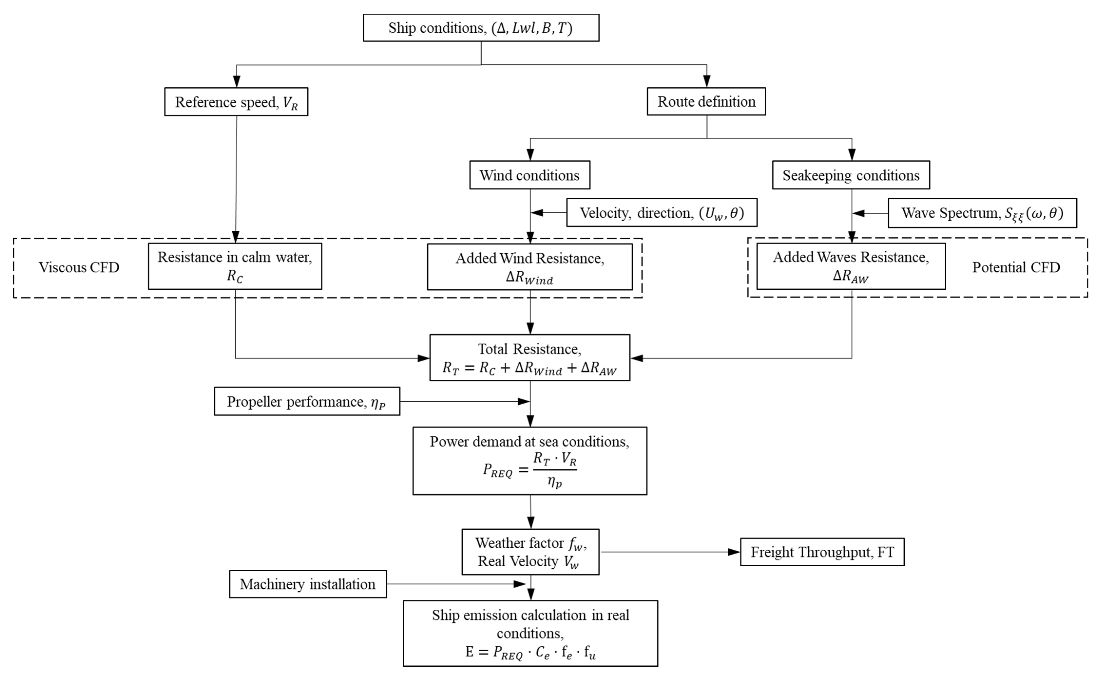
2. Aim of This Work and Methodology

This research analyzed a short sea shipping route between Mediterranean ports using high-fidelity commercial tools to assess the increase in ship emissions during navigation due to added resistance and the impact on ship freight throughput. To carry out this research, different high-fidelity numerical tools and approaches were used. In previous studies, low-fidelity tools were employed to carry out this task, or the use of high-fidelity tools was limited. A comparative study with different tools was addressed according to International Towing Tank Conference (ITTC) recommended practices [20] to value the importance of using high-fidelity tools in the whole view of ship navigation. RANS computations were carried out for bare hull analysis, added resistance in irregular waves was analyzed by a high order potential solver and an in-house numerical code based on semi-Lagrangian particle finite element method (SLPFEM) is used to determine wind added resistance.

The increase in ship emissions was determined through the speed loss calculation on a commercial route between Mediterranean ports. The methodology follows the ITTC recommendations to assess ship speed loss [20]. Components of added resistance were calculated using high fidelity numerical tools. Calm water resistance was first determined by the viscous solver Tdyn [21]. Added resistance in waves was solved using commercial code SeaFEM based on the work of García-Espinosa and Serván-Camas [22]. Then, the added wind resistance was calculated using the Fujiwara method and in-house code based on the semi-Lagrangian approach for the incompressible Navier–Stokes equations developed by Nadukandi et al. [23] and Colom-Cobb et al. [24]. Next, the propeller efficiency was corrected to account for the impact on the power demand. Then, the negative impact of added resistance on ship emissions and freight throughput could be determined for the route selected. Figure 1 shows an approach of the methodology to value the increase in ship emissions and the impact of the freight throughput. Details of each step in the added resistance calculation are given below.

3. Calculation of Weather Factor

3.1. Main Particulars and Ship Conditions

During 2018, roll on-roll off (Ro-Ro) units accounted for 249 million tons (14%) of the total short sea shipping of goods to and from the main European Union ports [25]. Short sea shipping has more frequent port calls, which in turn means that the price and quality of all port-related services and hinterland connections have a relatively larger impact than on deep sea operations. One of the defining differences between short sea and deep-sea shipping is that there are no alternatives to the latter. In contrast, short sea shipping often competes with other modes of transport, such as roads and rail [26]. That said, short sea shipping and other land-based modes often also cooperate in forming truly intermodal logistics chains [27]. These reasons led us to select a Ro-Ro ship to carry out the research. The main particulars, load conditions, and ship’s propeller parameters of the ship selected are shown in

Table 1. Main particulars of ship selected.

Particular	Value	Unit
Length overall	180.6	m
Beam	22.9	m
Depth	14.1	m
Displacement	14,918	Metric Tons
Deadweight	7500	Metric Tons
Block coefficient (Cb)	0.6
Power installed	11,600	kW
Velocity at 85% of MCR	18.0	Knots
Autonomy	8000	Milles

MCR = Maximum Continuous Rating. Source: Own elaboration.

,

Table 2. Load conditions used for total resistance calculation.

Particular	Load Condition 1	Load Condition 2	Unit
Displacement	14,312	15,526	Metric tons
Draught at Forward Perpendicular	5.69	6.04	m
Draught at After Perpendicular	5.98	6.32	m
Draught Amidships	5.83	6.18	m
Wetted area	4569	4784	m2
Vertical center of gravity	10.68	10.03	m
Transversal metacentric height a	1.92	2.42	m
Longitudinal metacentric height	478.73	454.39	m

^a Result with the free surface correction applied. Source: Own elaboration.

and

Table 3. Main parameters related to ship propeller.

Parameter	Value	Unit
Number of Blades (Z)	4
Diameter (m)	4.65	m
Extended–disc area ratio (Ae/Ao)	0.5
Pitch–diameter ratio (P/D)	1.4

Source: Own elaboration.

, respectively. Two load conditions are used for calculations (see Table 2).

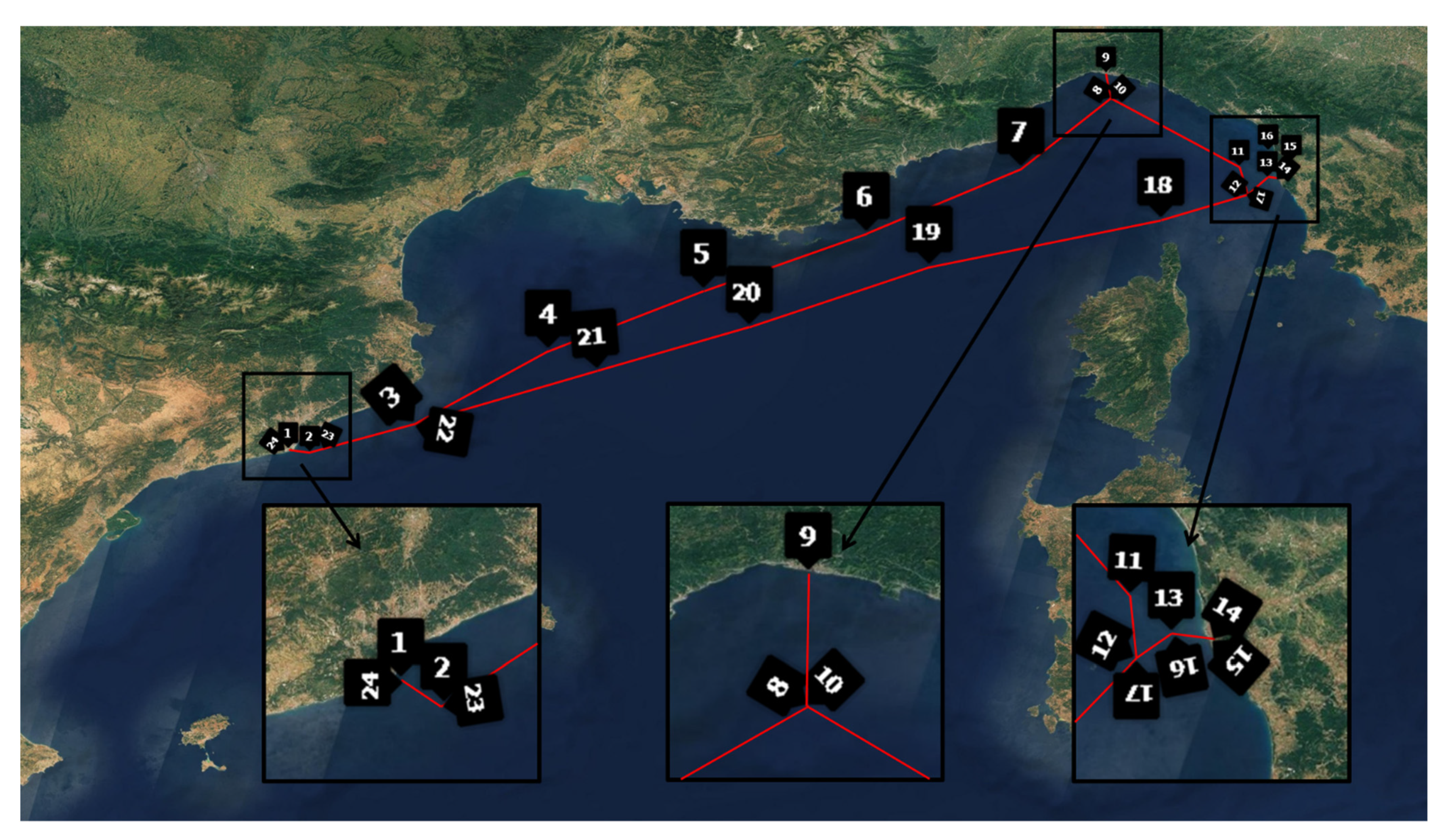
3.2. Route and Environmental Conditions

The selected ship navigates between the ports of Barcelona, Livorno and Genoa, which is one of the most active routes in the Western Mediterranean Sea (see Figure 2). These ports have a remarkable traffic of Ro-Ro units. During 2018, Livorno and Genoa had a throughput of 11.05 and 10.11 million tons of traffic in Ro-Ro units, respectively. Both represented the first and second ports in Italy with the highest Ro-Ro traffic in 2018. Barcelona had a throughput of 1.07 million tons, which represented the seventh busiest port in Spain [28].

To determine the added resistance, the route was split into 24 points of study (see Figure 2). Route way points are shown in

Table A1. Way points of sections of route selected (Barcelona–Genoa–Livorno–Barcelona).

Points	Latitude	Longitude
1	41°20.9′	002°11.1′
2	41°19.6′	002°13.6′
3	41°41.2′	003°28.1′
4	42°10.7′	004°38.3′
5	42°39.5′	005°49.8′
6	43°06.2′	007°02.8′
7	43°37.2′	008°13.2′
8	44°23.4′	009°02.5′
9	44°23.4′	008°56.4′
10	44°24.0′	008°54.6′
11	44°23.4′	008°56.7′
12	44°19.9′	008°58.0′
13	43°43.3′	010°04.0′
14	43°33.1′	010°10.2′
15	43°29.3′	010°12.8′
16	43°32.5′	010°17.4′
17	43°32.7′	010°17.1′
18	43°14.3′	009°27.8′
19	42°48.5′	007°29.4′
20	42°25.7′	006°02.8′
21	42°01.9′	004°38.5′
22	41°41.2′	003°28.1′
23	41°19.6′	002°13.6′
24	41°20.9′	002°11.1′

in Appendix A. The encountered weather conditions corresponding with sea states (SS) in each point were divided into four seasons, to account the influence of these upon added resistance. These were: December to February; March to May; June to August; and, September to November. Weather conditions along the route were extracted from the reanalysis of met-ocean data provided by Spanish National Meteorological Agency [29,30]. The wave fields were generated by WAM [31] and WaveWatch III models [32] fed by HIRLAM and HARMONIE-AROME wind model [29,33] in some route points. Values corresponding with each SS are shown in

Table A2. Sea state per route point in December to February season.

Points	Significant Height (m)	Peak Period (s)	Wave Heading (deg)	Wind Velocity (m/s)	Wind Heading (deg)
1	1.055	6.50	126.6	3.68	193.9
2	1.055	6.50	126.6	3.68	193.9
3	1.524	5.96	112.0	4.57	108.2
4	1.773	5.97	183.7	9.24	234.1
5	1.583	5.97	198.8	9.33	238.1
6	1.447	6.01	139.9	7.74	155.7
7	0.911	6.02	131.3	5.51	182.4
8	0.879	6.24	141.8	5.14	162.3
9	0.879	6.24	141.8	5.14	162.3
10	0.879	6.24	141.8	5.14	162.3
11	0.879	6.24	141.8	5.14	162.3
12	0.879	6.24	141.8	5.14	162.3
13	1.110	5.87	171.0	6.44	173.2
14	1.110	5.87	171.0	6.44	173.2
15	1.110	5.87	171.0	6.44	173.2
16	1.110	5.87	171.0	6.44	173.2
17	1.110	5.87	171.0	6.44	173.2
18	1.187	6.03	182.8	7.74	155.7
19	1.624	6.15	176.5	7.77	171.9
20	1.589	6.11	188.1	8.43	210.2
21	1.846	6.05	214.0	9.53	240.9
22	1.763	6.11	130.3	4.57	108.2
23	1.055	6.50	126.6	3.68	193.9
24	1.055	6.50	126.6	3.68	193.9

,

Table A3. Sea state per route point in March to May season.

Points	Significant Height (m)	Peak Period (s)	Wave Heading (deg)	Wind Velocity (m/s)	Wind Heading (deg)
1	0.960	5.99	131.7	3.98	150.5
2	0.960	5.99	131.7	3.98	150.5
3	1.273	5.86	107.3	4.29	118.9
4	1.468	5.58	207.4	7.31	210.4
5	1.323	5.54	205.4	6.72	210.1
6	1.176	5.60	174.2	6.60	142.1
7	0.827	5.69	136.2	4.60	180.8
8	0.820	6.03	141.5	4.07	165.7
9	0.820	6.03	141.5	4.07	165.7
10	0.820	6.03	141.5	4.07	165.7
11	0.820	6.03	141.5	4.07	165.7
12	0.820	6.03	141.5	4.07	165.7
13	0.981	5.77	184.7	5.29	162.7
14	0.981	5.77	184.7	5.29	162.7
15	0.981	5.77	184.7	5.29	162.7
16	0.981	5.77	184.7	5.29	162.7
17	0.981	5.77	184.7	5.29	162.7
18	1.022	5.80	189.0	6.60	142.1
19	1.316	5.74	184.5	6.49	153.1
20	1.306	5.68	192.8	6.33	180.1
21	1.519	5.63	215.7	7.22	210.8
22	1.438	5.76	127.6	4.29	118.9
23	0.960	5.99	131.7	3.98	150.5
24	0.960	5.99	131.7	3.98	150.5

,

Table A4. Sea state per route point in June to August season.

Points	Significant Height (m)	Peak Period (s)	Wave Heading (deg)	Wind Velocity (m/s)	Wind Heading (deg)
1	0.740	5.49	132.6	3.86	143.8
2	0.740	5.49	132.6	3.86	143.8
3	0.973	5.49	95.2	3.58	108.2
4	1.110	4.92	215.2	6.66	247.8
5	1.014	4.92	210.9	6.35	249.4
6	0.900	5.02	180.3	4.57	198.6
7	0.671	5.04	128.1	2.98	177.3
8	0.674	5.23	128.7	2.73	147.3
9	0.674	5.23	128.7	2.73	147.3
10	0.674	5.23	128.7	2.73	147.3
11	0.674	5.23	128.7	2.73	147.3
12	0.674	5.23	128.7	2.73	147.3
13	0.775	5.19	192.6	4.05	219.5
14	0.775	5.19	192.6	4.05	219.5
15	0.775	5.19	192.6	4.05	219.5
16	0.775	5.19	192.6	4.05	219.5
17	0.775	5.19	192.6	4.05	219.5
18	0.826	5.22	191.1	4.57	198.6
19	1.000	5.14	190.6	4.84	205.3
20	0.999	5.07	198.0	5.61	231.2
21	1.143	5.00	224.7	6.50	248.5
22	1.076	5.10	107.0	3.58	108.2
23	0.740	5.49	132.6	3.86	143.8
24	0.740	5.49	132.6	3.86	143.8

and

Table A5. Sea state per route point in September to November season.

Points	Significant Height (m)	Peak Period (s)	Wave Heading (deg)	Wind Velocity (m/s)	Wind Heading (deg)
1	0.970	6.13	124.3	3.58	167.0
2	0.970	6.13	124.3	3.58	167.0
3	1.293	5.82	101.4	4.57	115.5
4	1.471	5.56	194.4	7.32	223.0
5	1.323	5.53	194.2	7.23	220.7
6	1.196	5.50	163.9	5.86	151.7
7	0.817	5.04	123.9	4.51	192.5
8	0.812	5.80	128.9	4.58	157.8
9	0.812	5.80	128.9	4.58	157.8
10	0.812	5.80	128.9	4.58	157.8
11	0.812	5.80	128.9	4.58	157.8
12	0.812	5.80	128.9	4.58	157.8
13	0.981	5.19	164.5	5.12	168.1
14	0.981	5.19	164.5	5.12	168.1
15	0.981	5.19	164.5	5.12	168.1
16	0.981	5.19	164.5	5.12	168.1
17	0.981	5.19	164.5	5.12	168.1
18	0.996	5.59	169.9	5.86	151.7
19	1.304	5.61	171.4	5.86	160.9
20	1.302	5.61	181.1	6.47	192.6
21	1.517	5.62	205.0	7.31	222.1
22	1.452	5.71	113.5	4.57	115.5
23	0.970	6.13	124.3	3.58	167.0
24	0.970	6.13	124.3	3.58	167.0

in Appendix A. The data provided were analyzed to obtain those required as input data for numerical simulations. They were: significant wave height (H_s), peak period (T_p), wave heading (θ), wind velocity (V_w), and wind heading (β).

The following analysis is based on 96 SS (24 points × 4 seasons). They are combined with three Froude numbers of: 0.16 (12 knots), 0.20 (15 knots), and 0.24 (18 knots) corresponding with those reference velocities in which the added resistance will be computed. The ship total resistance (R_t) can be split into three terms, which are determined for each route point:

$$R_t=R_c+\Delta R_{AW}+\Delta R_W,$$

(1)

where $R_c$ is the calm water resistance, $\Delta R_{AW}$ is the added resistance in waves, and $\Delta R_W$ is the added resistance of wind. Next, each term of added resistance will be computed.

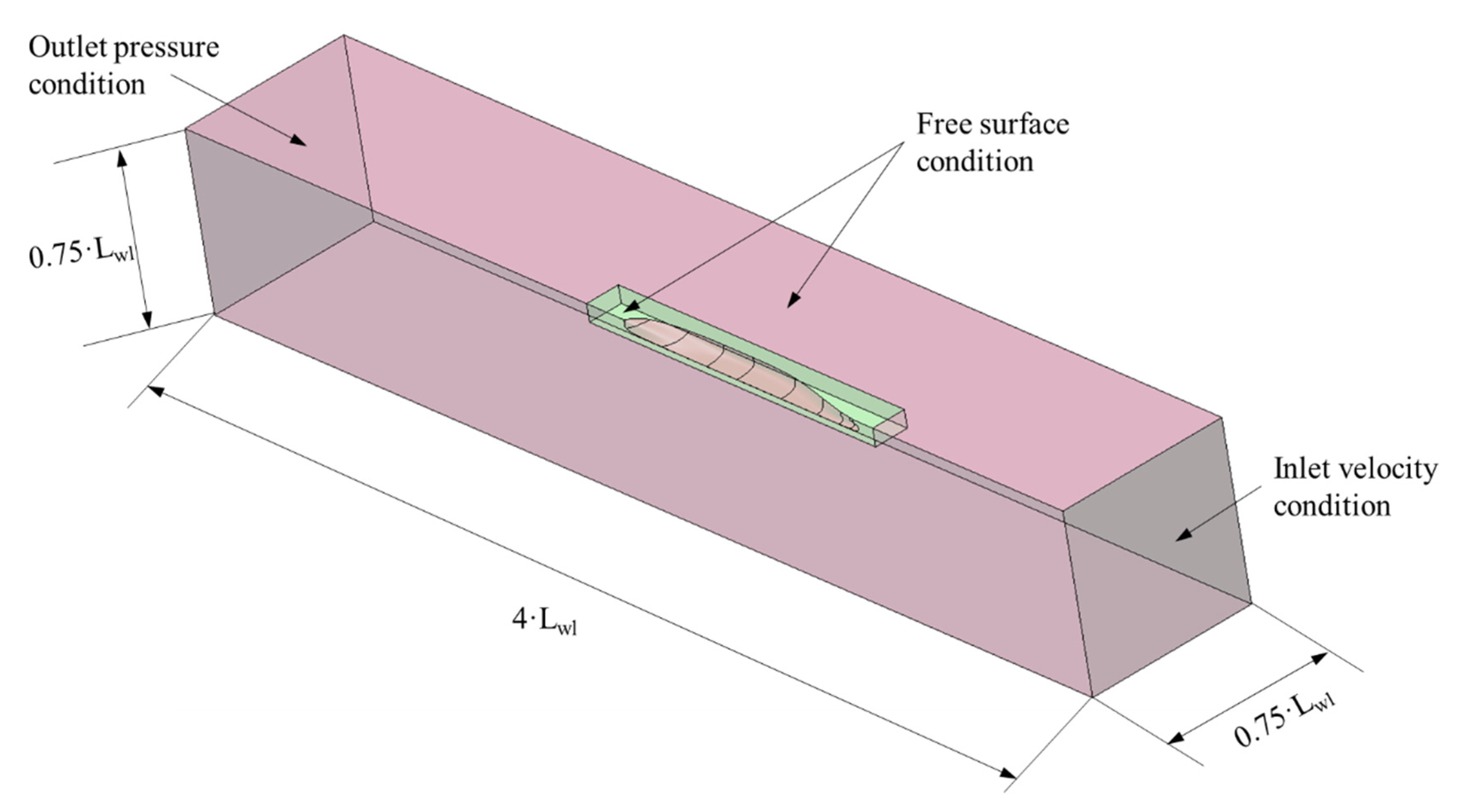
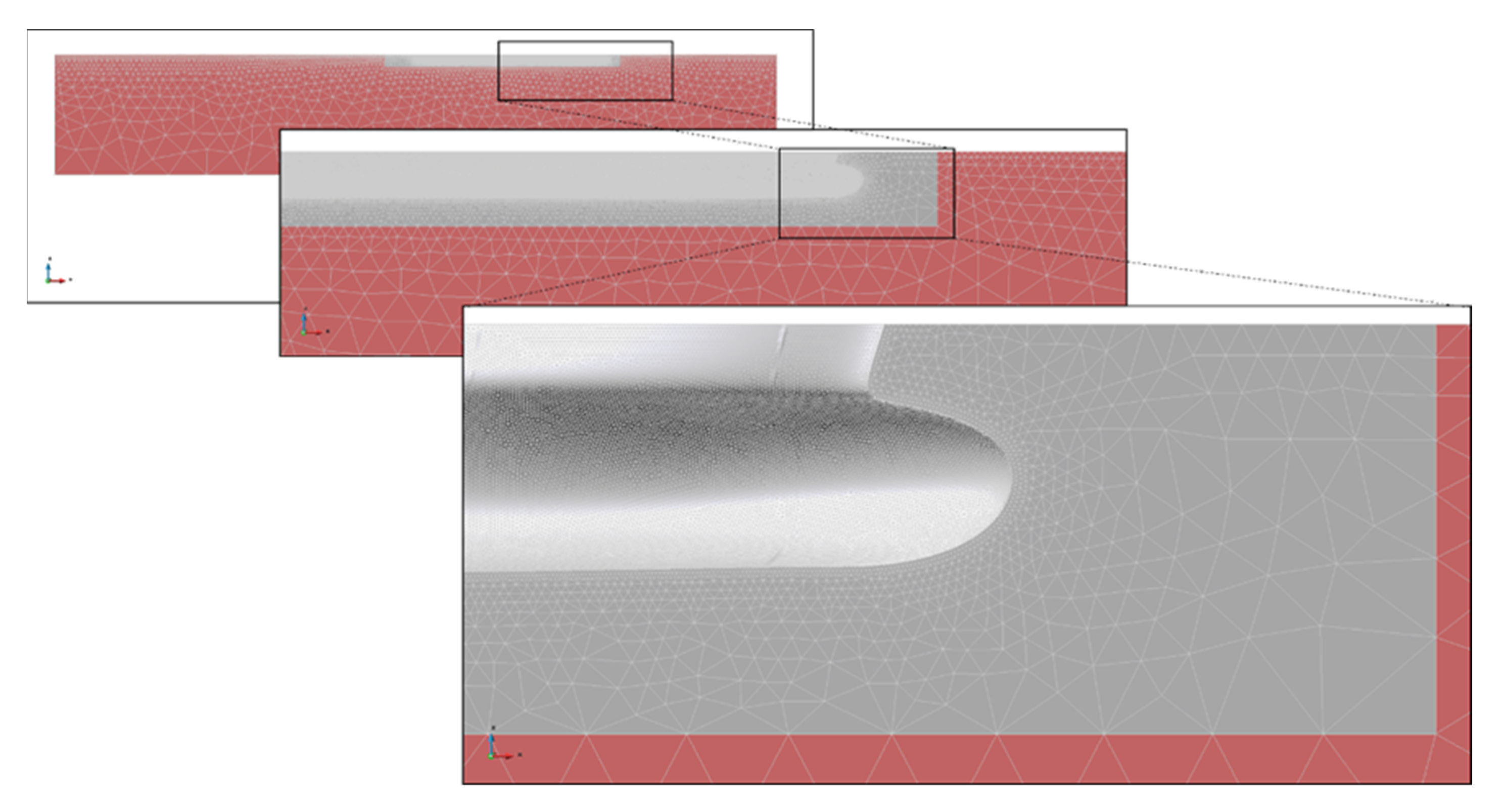
3.3. Calm Water Resistance

Experimentation in towing tanks should be performed anyway. However, for practical issues, ITTC pointed out that the CFD approach should also be used [20]. Resistance in calm water is determined using the commercial code Tdyn based on time-averaged Navier–Stokes equations solved by the finite element method [21,34]. The description and details of the numerical model used can be found in CompassIS [21] and García-Espinosa and Oñate [34].

For calm water resistance computations, the SST version of the k-ω turbulence model [35,36] has been employed to simulate the turbulent flow around the bare hull. Three-dimensional numerical results were obtained using a right-handed coordinate system. Regarding the boundary conditions, the inlet velocity condition is applied at the entrance of the domain (right side in Figure 3). At the outlet section (left side of Figure 3), the pressure is assumed to be equal to the atmospheric pressure. The no-slip condition is applied for velocities and turbulent variables at the solid walls. Regarding the turbulence simulation, the intensity turbulence for external flow is usually fixed at 1%, and delta wall modelling is used for near-wall treatment. Y plus number equal to 30 is used for wall treatment and to satisfy a logarithmic profile assumption.

To reduce the number of mesh elements, a half hull has been considered and, therefore, the symmetry condition is imposed into the boundary conditions (Figure 3 shows a general arrangement of the control volume used). Mesh dependence analysis is performed for Load Condition 1 and Froude number equal to 0.16. The results are shown in Figure 4. Details of size of the grids on boundaries are shown in

Table 4. Details of unstructured mesh sizes applied to computational domain for CFD computation.

Element	Size (mm)
Hull surface	1.0
Inner free surface	8.0
Outer free surface	20.0
General size	30.0

Source: Own elaboration.

. An example of unstructured mesh elements for each simulation performed can be observed in Figure 5. Additional details about the fundamentals of the employed models can be found in CompassIS [21].

The time-dependent procedure is employed for obtaining the numerical results, with time steps on the order of 0.01 s with a Courant number of 0.01 with 10,000 steps of simulation. Numerical convergence is assumed when the residuals of governing equations are below 10⁻⁷ in each iteration.

Table 5. Values of bare hull resistance in kilonewtons (kN) for CFD computations, Holtop and Mennen’s and Fung and Liebman methods.

Fr	LC 1 (CFD)	LC 1 (HM)	LC 1 (FL)	LC 2 (CFD)	LC 2 (HM)	LC 2 (FL)
0.16	253.9	221	175	240.4	211	168
0.20	325.9	401	325	335.2	384	313
0.24	517.0	610	512	505.6	584	495

LC = Load Condition; HM = Holtrop and Mennen’s method; FL = Fung and Liebman’s method. Source: Own elaboration.

shows the results for bare hull resistance. The values of each computation of time series were averaged.

Computational simulations were carried out with a model scale of 1:50. Then, the Prohaska [35] correlation method is applied to obtain the calm water resistance in the full-scale model.

In order to verify calm water resistance obtained from CFD calculation a comparison with Holtrop and Mennen’s [37,38] and Fung and Liebman [39] empirical methods are addressed (see Table 5). Holtrop and Mennen’s and Fung and Liebman’s methods gave similar results, but overestimated the bare hull resistance if the values were compared with CFD.

3.4. Added Resistance in Waves

The computation of added resistance in irregular waves requires the calculation of added resistance in regular waves first. Added resistance in irregular waves can be formulated as [40]:

$$\Delta R_{AW}=2{{\displaystyle \int }}_0^{\infty }{{\displaystyle \int }}_0^{2\pi }\frac{R_{AW}\left(\omega ,\alpha ;U\right)}{{\xi }^2}E\left(\omega ,\alpha ;H,T,\theta \right) \mathrm{d}\alpha \mathrm{d}\omega ,$$

(2)

where $R_{AW}\left(\omega ,\alpha ;V\right)$ is the added resistance induced by ship motion in regular waves for each frequency, $E\left(\omega ,\alpha ;H, T,\theta \right)$ is the directional sea spectrum [20,40], $\omega$ is the circular frequency of incident regular waves, $\alpha$ is the angle between ship course and regular waves, U is the ship speed, $\xi$ is the wave amplitude, $H$ is the significant wave height, T is the mean wave period and $\theta$ is the mean wave direction.

The calculation of added resistance is performed using the SeaFEM potential code [41], which is based on the work of García-Espinosa and Servan-Camas [22]. The computation is in the time domain, using the finite element method with unstructured meshes based on second order of radiation-diffraction model. Some details about the computation are given below.

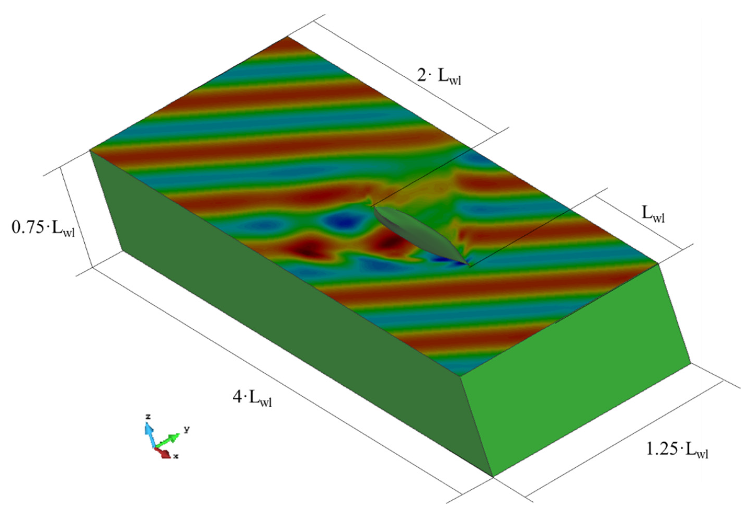
3.4.1. Convergence Analysis

Studying the influence of the different unstructured mesh densities in the results is mandatory to obtain an accurate analysis with reasonable computational cost. Six meshes are tested for Froude number equal to 0.2 in regular waves with wavelength equal to waterline length and with 1 m of wave amplitude. The computations are performed for the Load Condition 2. Infinite depth is considered for the analysis. The Sommerfeld radiation condition occurs at the edge boundary [41]. The size of the computational domain is shown in Figure 6.

Table 6. Relative error for different meshes of dimensionless added wave resistance in regular airy waves.

Mesh	Wetted Surface Mesh Size (M)	Inner Surface Mesh Size (M)	Outer Surface Mesh Size (M)	$\frac{{\mathit{R}}_{\mathit{a}\mathit{w}}}{\mathit{\rho }\mathit{g}{\mathit{\xi }}^{\mathbf{2}}{\mathit{B}}^{\mathbf{2}}/{\mathit{L}}_{\mathit{w}\mathit{l}}}$	Relative Difference (%)	Number of Elements (×105)
1	2.0	2.0	6.0	13.74		1.05
2	1.5	2.0	6.0	5.20	62	1.46
3	1.5	1.5	4.0	6.09	17	1.48
4	1.0	1.5	4.0	6.07	0.3	1.55
5	1.0	1.0	2.0	5.67	1.8	1.91
6	0.5	0.5	2.0	6.22	0.7	10.75

Source: Own elaboration.

provides the dimensionless added resistance in waves, the difference between two consecutive discretization sizes, and the relative difference with respect to the corresponding resistance. Differences have been calculated instead of errors due to the lack of an exact solution to compare with. Additionally, details of mesh refinement are given in Table 6.

It can be noted that meshes from 3 to 6 offer similar results. Therefore, mesh number four is selected for regular wave computations.

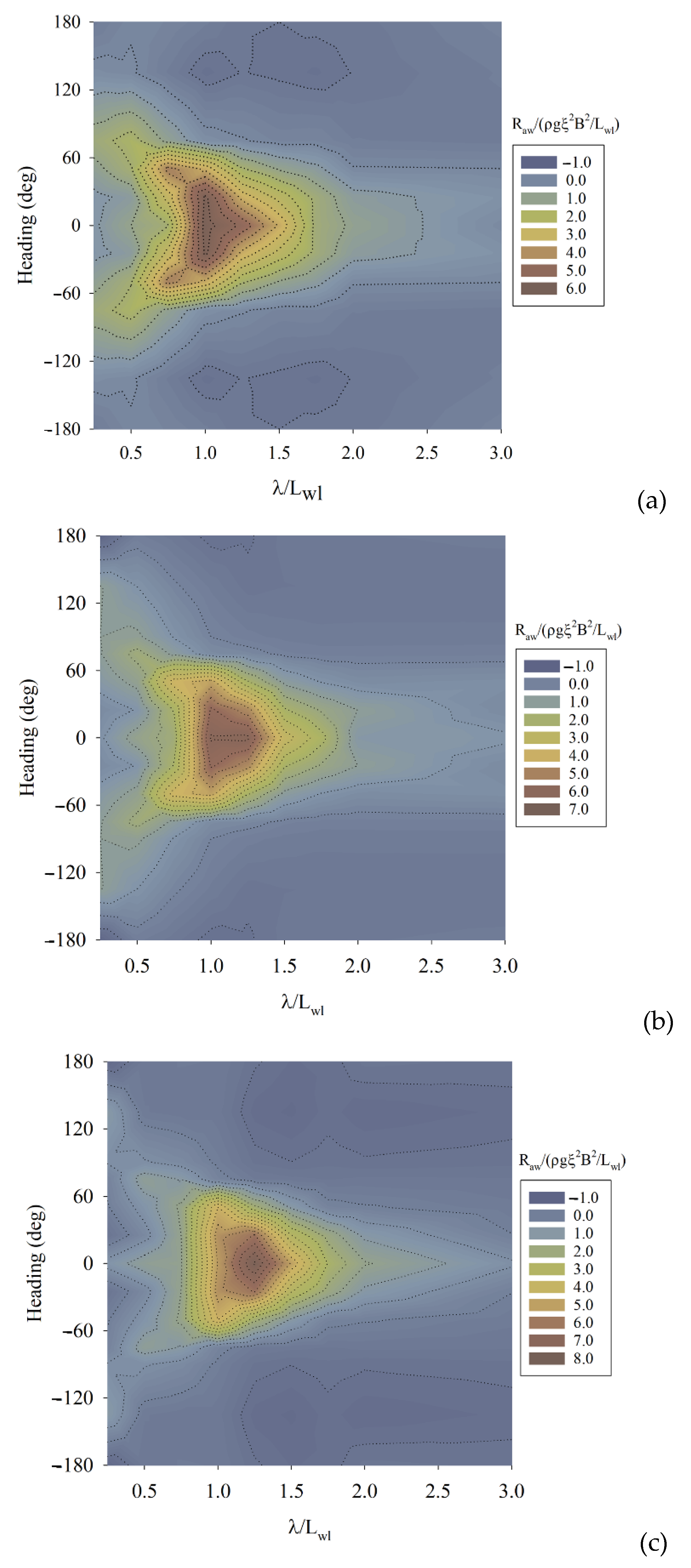
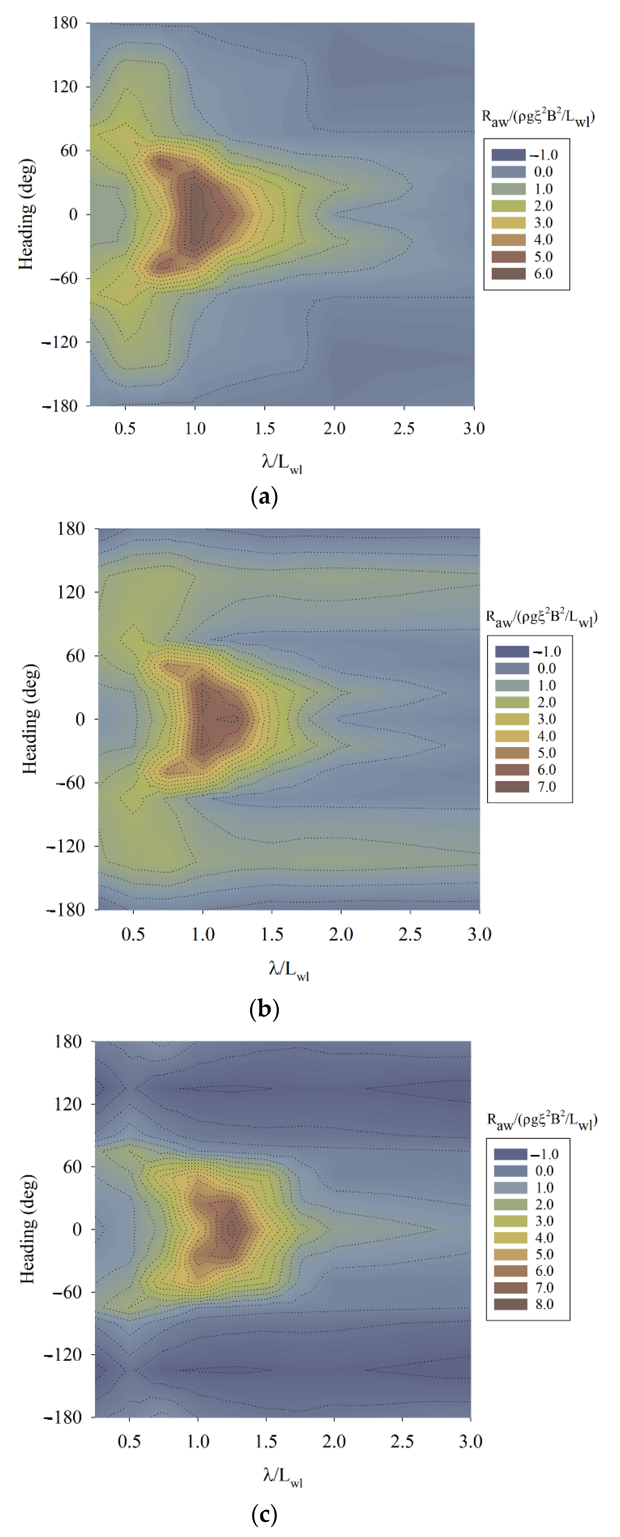
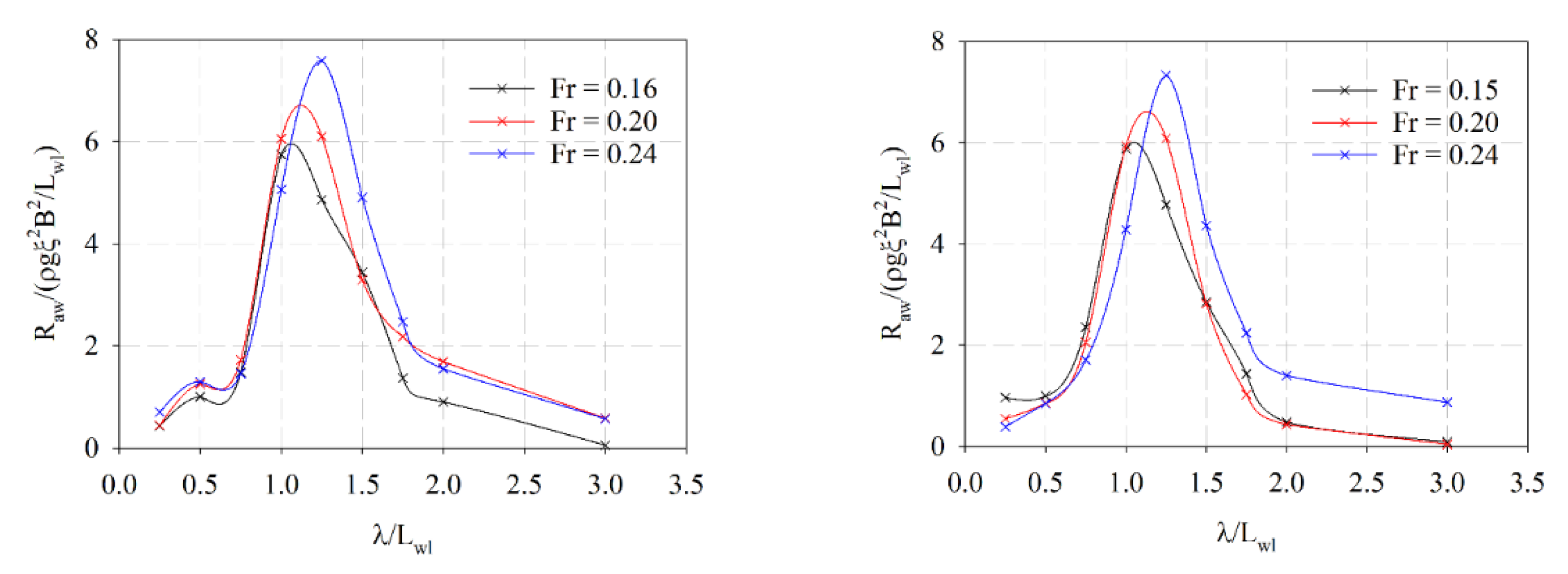
3.4.2. Results of Added Resistance in Regular Waves

The added resistance in regular waves for two load conditions is then determined. Wave lengths are in a range between 0.25 and 3.0 of dimensionless wavelength $\left(\lambda /L_{wl}\right)$, where L_wl is the waterline length in steps of 0.25. Computations for different wave headings to account for the influence of relative angle between ship course and waves are performed. The calculations are carried out for three velocities, to assess speed loss. These wave headings are in a range between 0 to $\pi$ radians in steps of $\raisebox{1ex}{$5\pi $}\!\left/ \!\raisebox{-1ex}{$36$}\right.$ rad. Results of dimensionless added wave resistance for three velocities are shown in contour line plots in Figure 7 and Figure 8. These figures are the results of combinations of all cases computed, more than 100 cases per analyzed velocity. Intermediate values are linear interpolated.

Figure 9 shows the dimensionless added resistance versus dimensionless wavelength for two conditions and three Froude numbers analyzed for head waves. As can be noted, peak values are moved due to encountered frequency.

As can be noticed from Figure 7 and Figure 8, the added wave resistance becomes important in the range of spreading angle around 60 degrees. Negative values are obtained for following waves. This fact indicates that, in some cases, following waves could help the ship during its course. However, the negative values of added wave resistance may be considered as insignificant if they are compared with the values of bare hull resistance.

3.4.3. Results of Added Resistance in Irregular Waves

According to IMO [40] and the recommended procedures of ITTC [20], added resistance in irregular waves also applies in the case under study. Applying the IMO Spectrum, the added resistance in irregular waves is determined per each route point, and per each SS according to Equation (2). The results of added resistance in irregular waves for Froude number equal to 0.24 are presented in Figure 10. As can be seen, the worst conditions are found in the season December to February.

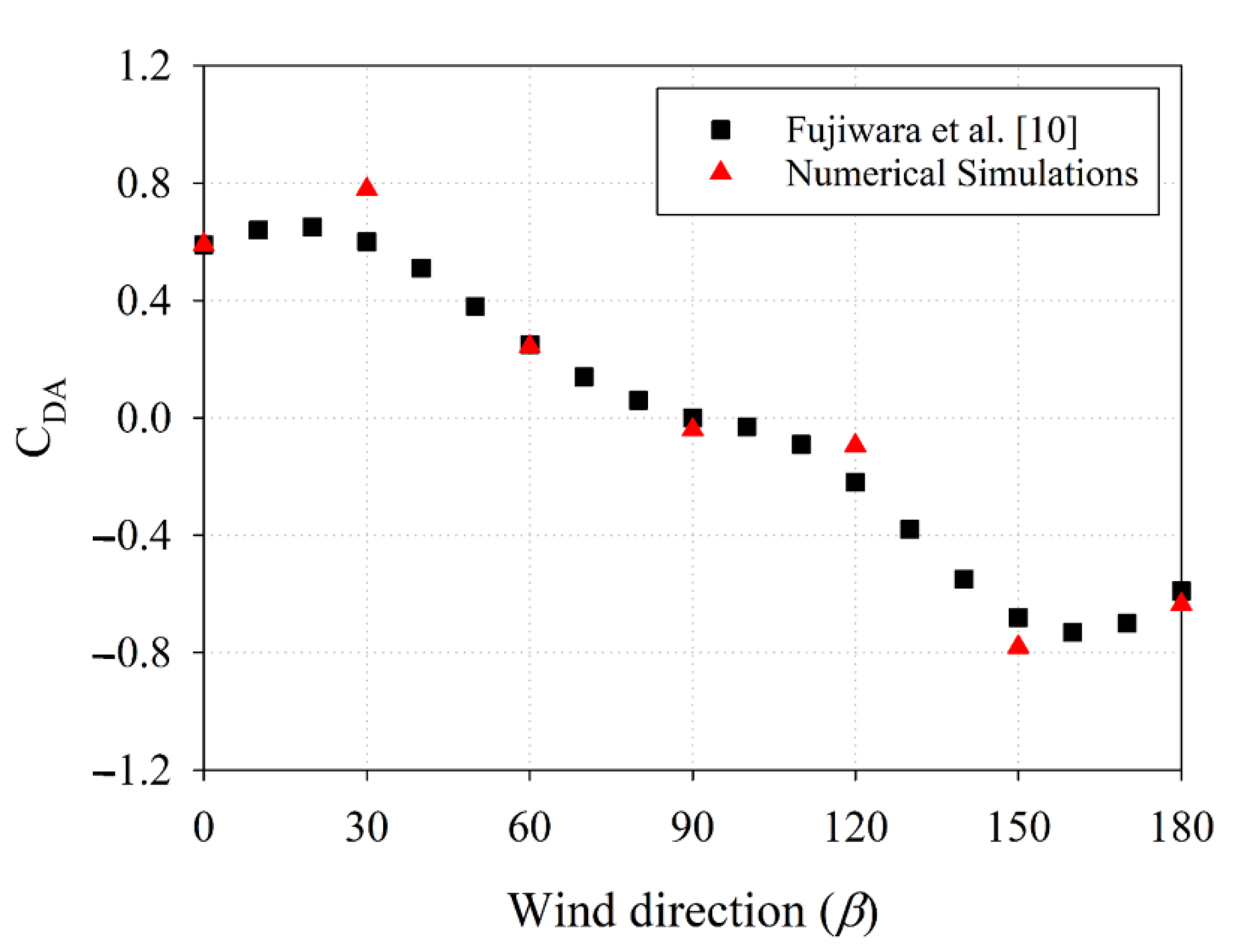
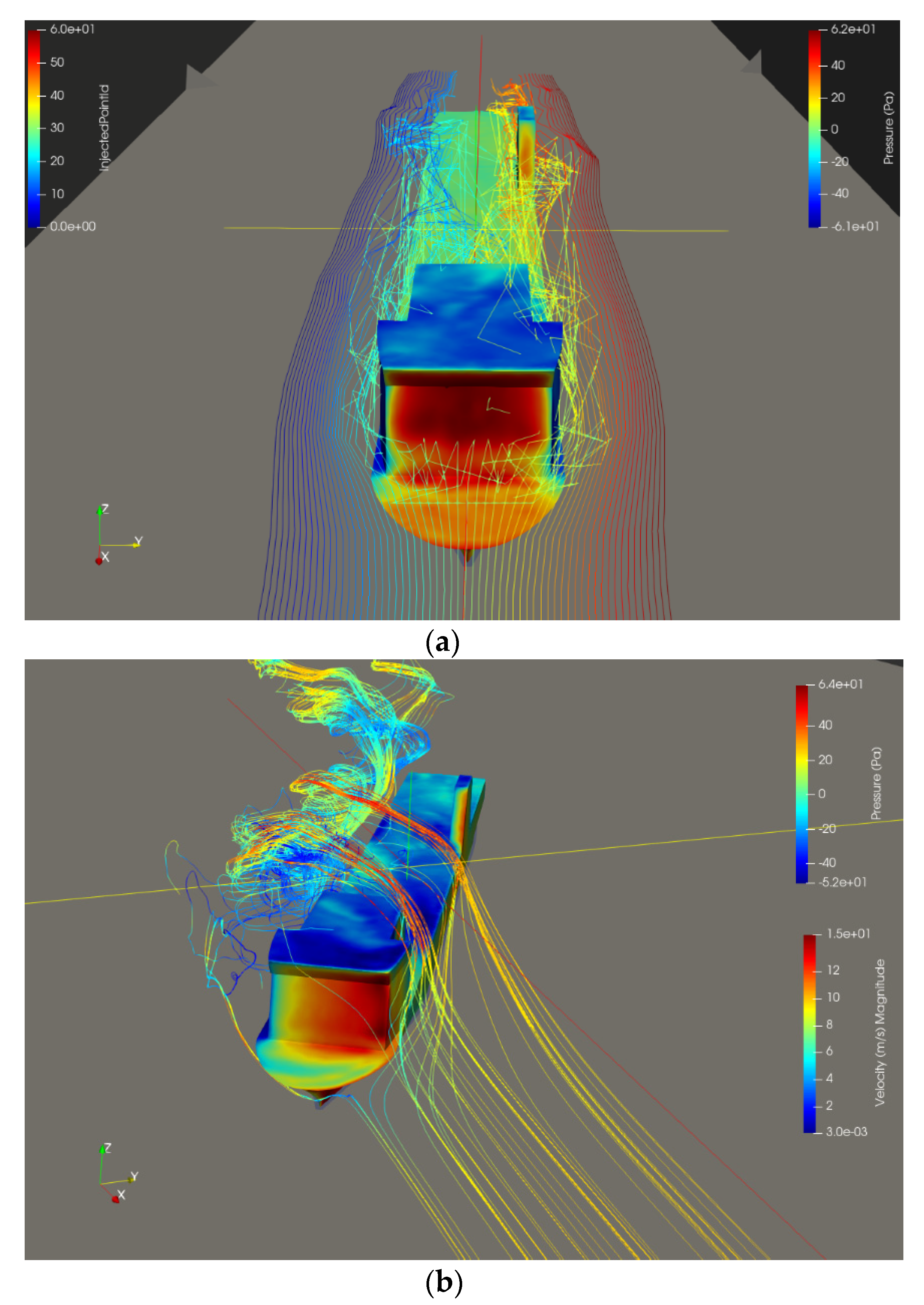
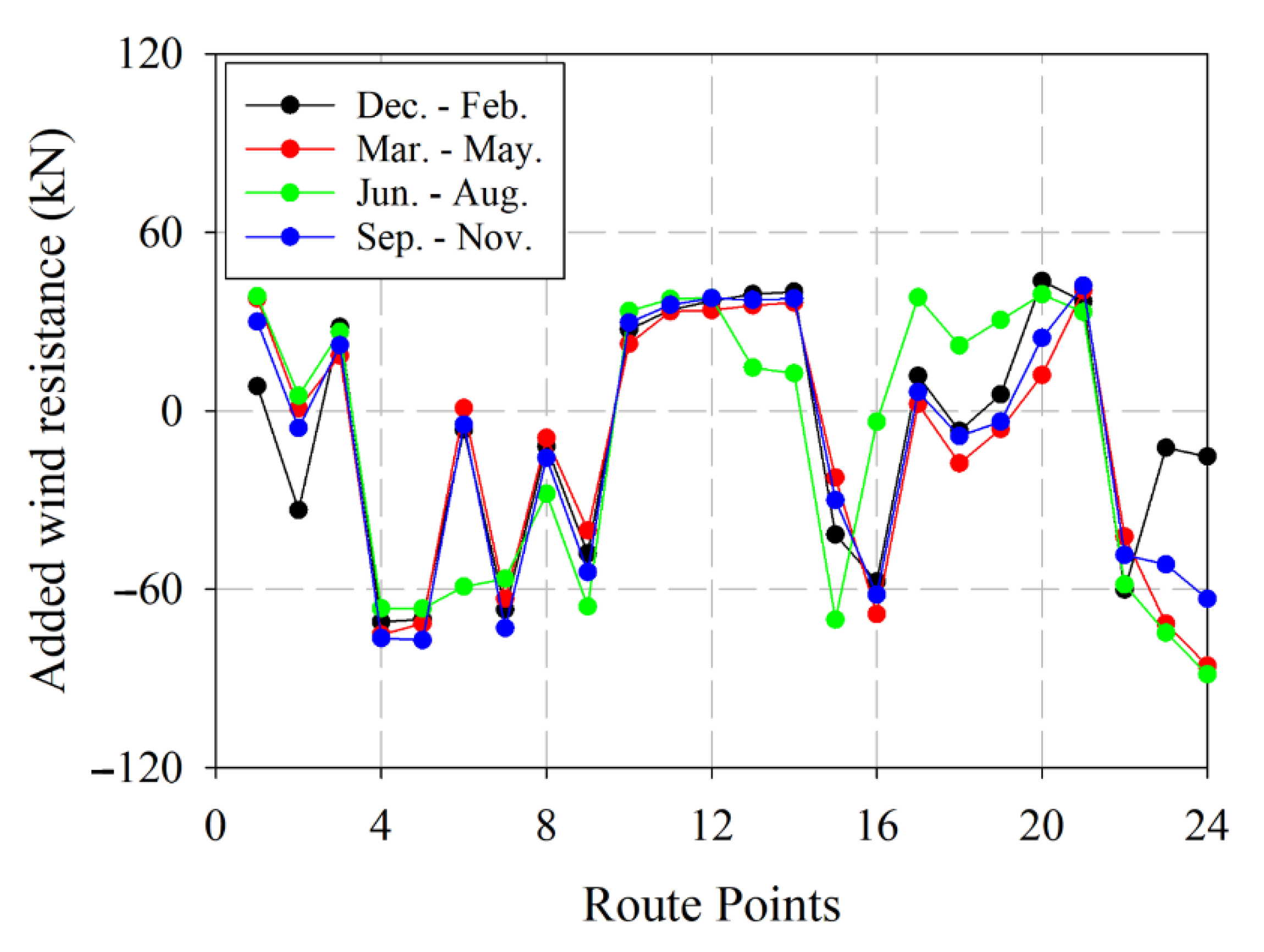
3.5. Wind-Added Resistance

As pointed out in the introduction, wind forces should be determined to consider all resistance components that act in ship navigations. The added wind resistance was calculated by accounting for the relative velocity between the ship course and wind direction. The Fujiwara method [10] can be used to determine the wind force coefficient (C_DA) depending on the apparent wind angle according to ITTC procedures [20]. The added wind resistance can be calculated as:

$$\Delta R_W=\frac{1}{2}{\rho }_{a}S{C}_{DA}\left(\beta \right)U_{rel}^2-\frac{1}{2}{\rho }_{a}S C_{DA}\left(0\right)U_{ref}^2,$$

(3)

where ${\rho }_a$ is the air density, S is the area of the maximum transverse section exposed to wind, $C_{DA}\left(\beta \right)$ is the wind force coefficient depending on the apparent wind angle, $U_{rel}$ is the apparent wind velocity, and U_ref is the design ship speed when ship is in operation in calm waters.

CFD computations are considered practical in comparison with empirical formulations [20]. The Fujiwara method [10] is compared with the in-house code based on the SLPFEM developed by Nadukandi et al. [23] and Colom-Cobb et al. [24]. Details about the parameters required for the Fujiwara method are given in

Table 7. Non-wetted surface parameters required for the Fujiwara regression method.

Parameter	Value	Unit
Lateral projected area of superstructures, deckhouses, etc. on deck (AOD)	450.6	m2
Area of maximum transverse section exposed to the winds (AXV)	315.8	m2
Projected lateral area above the waterline (AYV)	1337.0	m2
Horizontal distance from midship section to center of lateral projected area AYV (CMC)	0.9	m
Height of top of superstructure (navigation bridge, etc.) (hBR)	17.5	m
Height from waterline to center of lateral projected area AYV (hC)	6.7	m
Smoothing range; normally 10 (deg.) (μ)	0	deg
Relative wind direction; 0 means heading winds (ψWR)	180	deg

Source: Own elaboration.

.

In a literature review, similar studies can be found. For instance, in Janssen et al. [42], extensive research on the influence of simplification on CFD studies led to highly detailed ship analysis and high accuracy in the numerical results. For this investigation, a highly detailed ship model was modelled to perform numerical simulations.

The results obtained by the in-house numerical tool [23,24] are compared with the results obtained by the Fujiwara regression method. Regarding boundary conditions, a non-slip wall layer was used to compute pressure on ship surfaces. An exponential inflow wind profile with a reference value of 10 m/s is used to determine the added wind resistance coefficients. For each computation, more than 1.8 × 10⁷ unstructured mesh elements have been employed.

Figure 11 shows the values of the wind force coefficient obtained by the Fujiwara regression method versus the values obtained by numerical simulations. Similar results are achieved. Screenshots of streamlines of wind flow and pressure on ship surfaces from CFD computation are shown in Figure 12.

In this investigation, the Fujiwara method is used to determine the added wind resistance in the intermediate values because the results are very similar to those of numerical simulations. Figure 13 shows the values in kilonewtons per each route point and per season considered. Negative values indicate that the wind forces are on the same course as the ship.

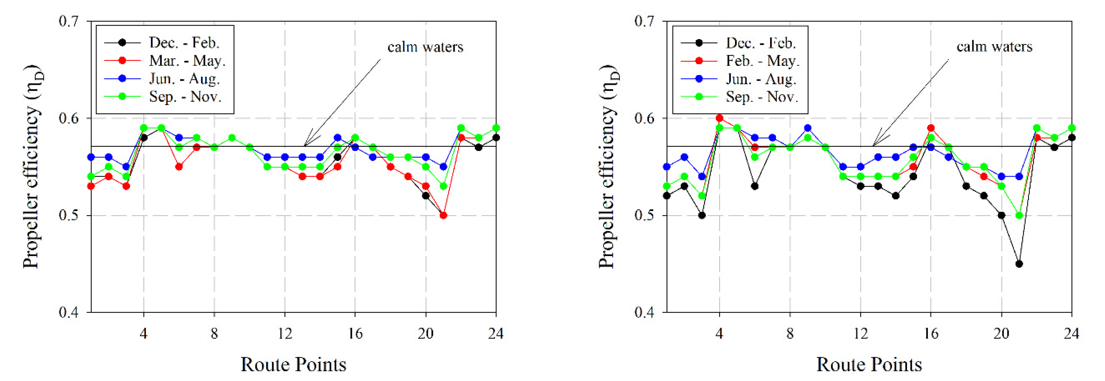
3.6. Propeller Efficiency

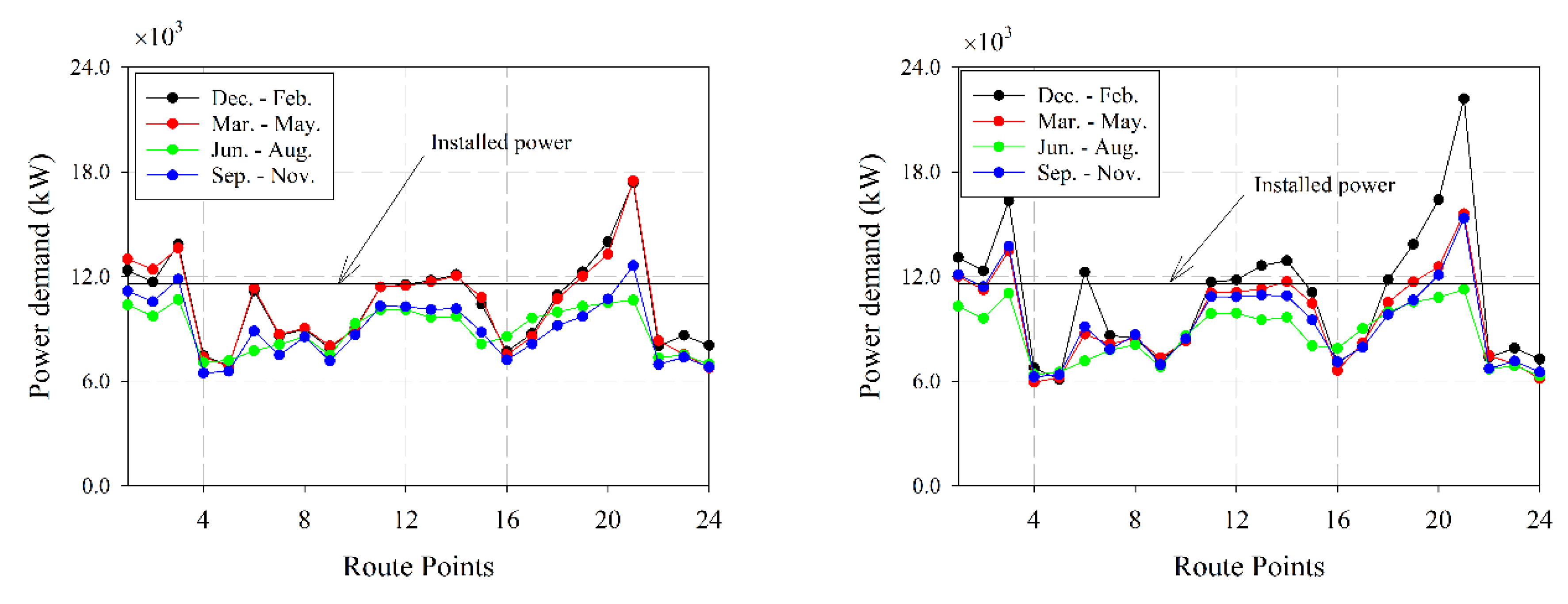
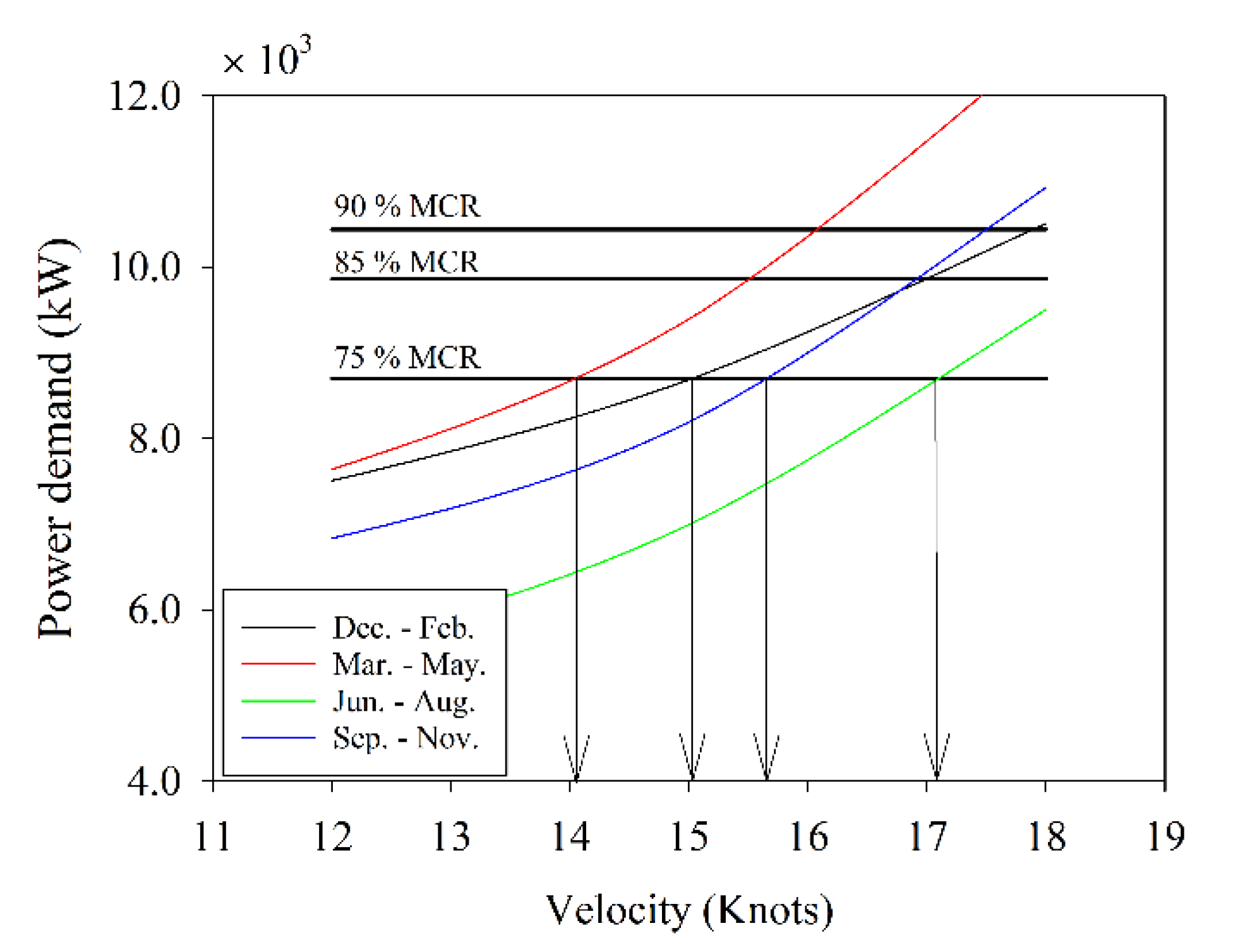
The power demand depends on propeller efficiency ${\eta }_D$, so this should also be considered. Table 3 shows the main particulars of the propeller considered for this work. The objective of this work is to consider all actions influencing pollutant emissions and ship freight throughput. Propeller efficiency can be significantly influenced by sailing in waves. The mechanical performance $\left({\eta }_M\right)$ is considered constant with a value of 0.95. Hull efficiency in calm water $\left({\eta }_H\right)$ is computed using the Holtrop and Mennen [37,38] formulation for each velocity. The same formulation is used to calculate rotative-relative efficiency $\left({\eta }_R\right)$, and it is assumed to be constant with a value of 0.958. Faltinsen et al. [43] noted no conclusions about the influence of waves in ${\eta }_R$. The open water propeller efficiency $\left({\eta }_o\right)$ is determined according to the Wageningen systematic series [44]. Propeller revolutions for this purpose are considered constant at 103 revolutions per minute (RPM). For our purpose, a reduction in propeller efficiency will be included in the model to evaluate the dynamic effects of waves on propeller efficiency. If the most likely wavelength is compared with the ship length and the most likely wave amplitudes are considered, losses regarding propeller ventilation can be assumed. Linear variation of propeller efficiency depending on added resistance is considered [45]:

$${\eta }_D={\eta }_D^0\left(\epsilon \frac{\Delta R_{AW}+\Delta R_W}{R_c}+1\right),$$

(4)

where $\epsilon$ is the overload factor with a value of −0.18. Similar results can be found in work by Taskar et al. [46] for wave amplitudes and wavelengths.

Figure 14 shows the variation of propeller efficiency per each load condition, per season, and per route point considered. The propeller efficiency increases because in some route points added resistance becomes negative, and the correction is linearly dependent on added resistance. Rough weather conditions negatively affect propeller efficiency, as can be seen in Figure 14 for Load Condition 2 during the season December to February.

3.7. Power Demand

Next, the power demand per route point is analyzed. As noted above, two load conditions and four seasons are considered to assess power demand. Figure 15 shows the values of power required for a Froude equal to 0.24 per each point and per season. The highest values are computed for Load Condition 2, in the season December to February, as expected.

4. Speed and Time Loss Calculation

According to the International Maritime Organization (IMO) [47], the weather factor of speed loss is influenced by weather in ship navigation. Speed loss $f_w$ is valued as:

$$f_w=\frac{speed considering weather}{speed in calm water}=\frac{U_W}{U_{ref}},$$

(5)

where U_W is the ship speed sailing in sea conditions, and U_ref is the ship speed sailing in calm waters.

The ITTC procedure [20] recommends the worst scenario, in which the wave and wind encounter angle gives the highest value of speed loss. In this investigation, speed loss is obtained per each route point and per season to give a full view of whole speed losses in a voyage. If speed loss is determined along ship course, then the time loss can be calculated accurately.

To compute the speed loss, a cubic function should be defined in order to know the intersection between nominal Maximum Continuous Rating (MCR) line and power demand curve. An example of the speed loss calculation for Load Condition 2 is presented in Figure 16. The intersection between the reference line of MCR and the resistance-velocity curve gives the speed loss.

The values of the speed losses ($f_w$) per each point, per load case and per considered season are determined. Different values of MCR for reference speeds are considered, taking into account that power regimes can change along ship voyage. Then, the time losses per season and load condition are determined. Only navigation time is considered in this stage. The values of navigation time per season and per load condition are shown in

Table 8. Voyage time per season, per Load Condition and per Maximum Continuous Rating (MCR) considered, compared with reference time in calm waters.

MCR (%)	75		80		90
Load Condition	1	2	1	1	2	1
December–February (h)	72.5	74.1	63.5	72.5	74.1	63.5
March–May (h)	56.6	64.2	54.4	56.6	64.2	54.4
June–August (h)	48.0	49.4	46.8	48.0	49.4	46.8
September–November (h)	56.8	61.7	51.3	56.8	61.7	51.3
Reference Time (h)	48.5		46.4		45.8

Source: Own elaboration.

.

As can be noted in Table 8, the highest speed losses are obtained in the season December to February, in both load conditions, when the worst environmental conditions are faced by ships. However, the ship can maintain the cruise speed in the season June to August, as can be noted. Lower differences are found between reference time and time per voyage in the season June to August in both conditions. Then, the influence of the added resistance on the ship emissions and the freight throughput is analyzed.

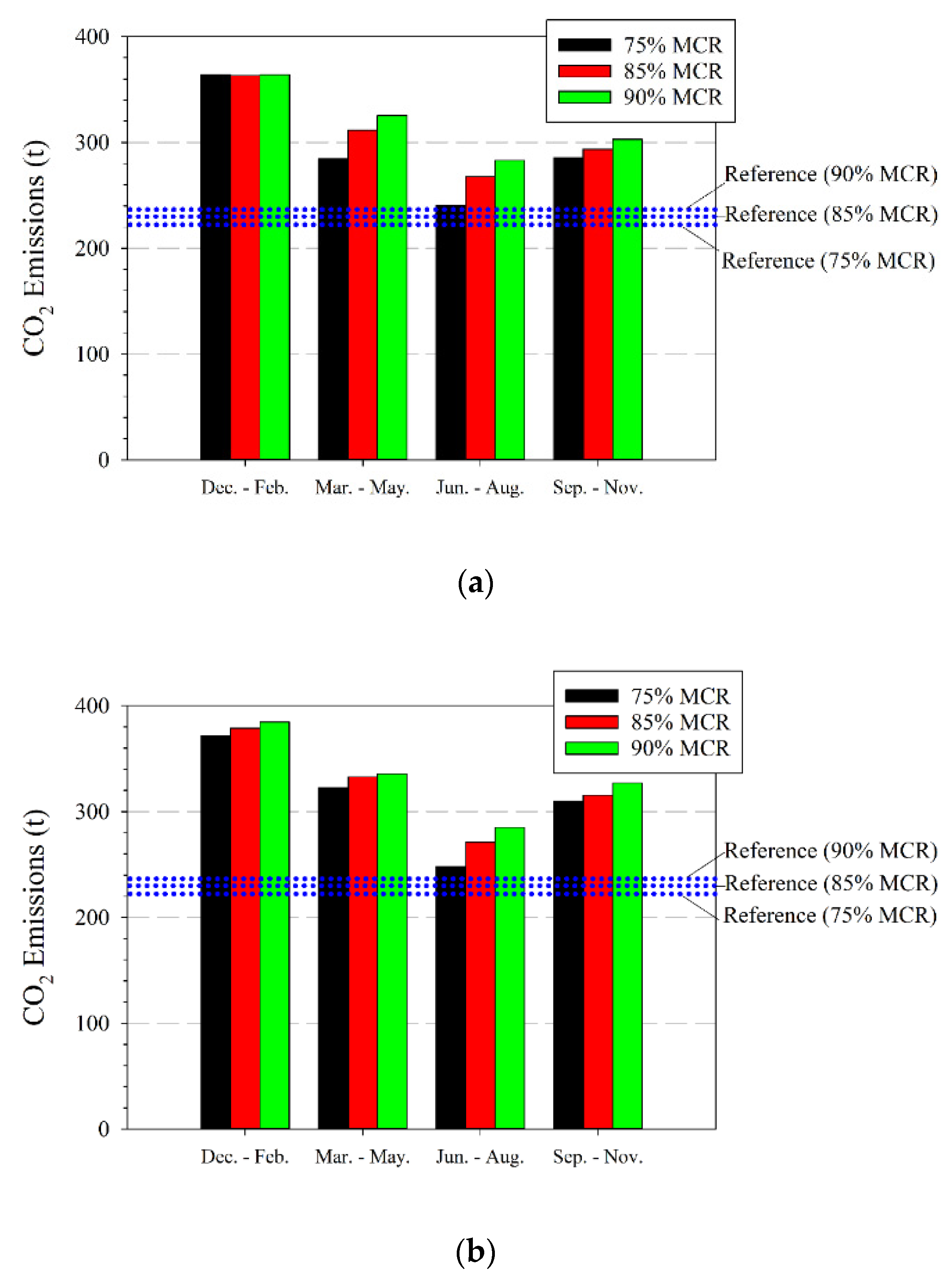
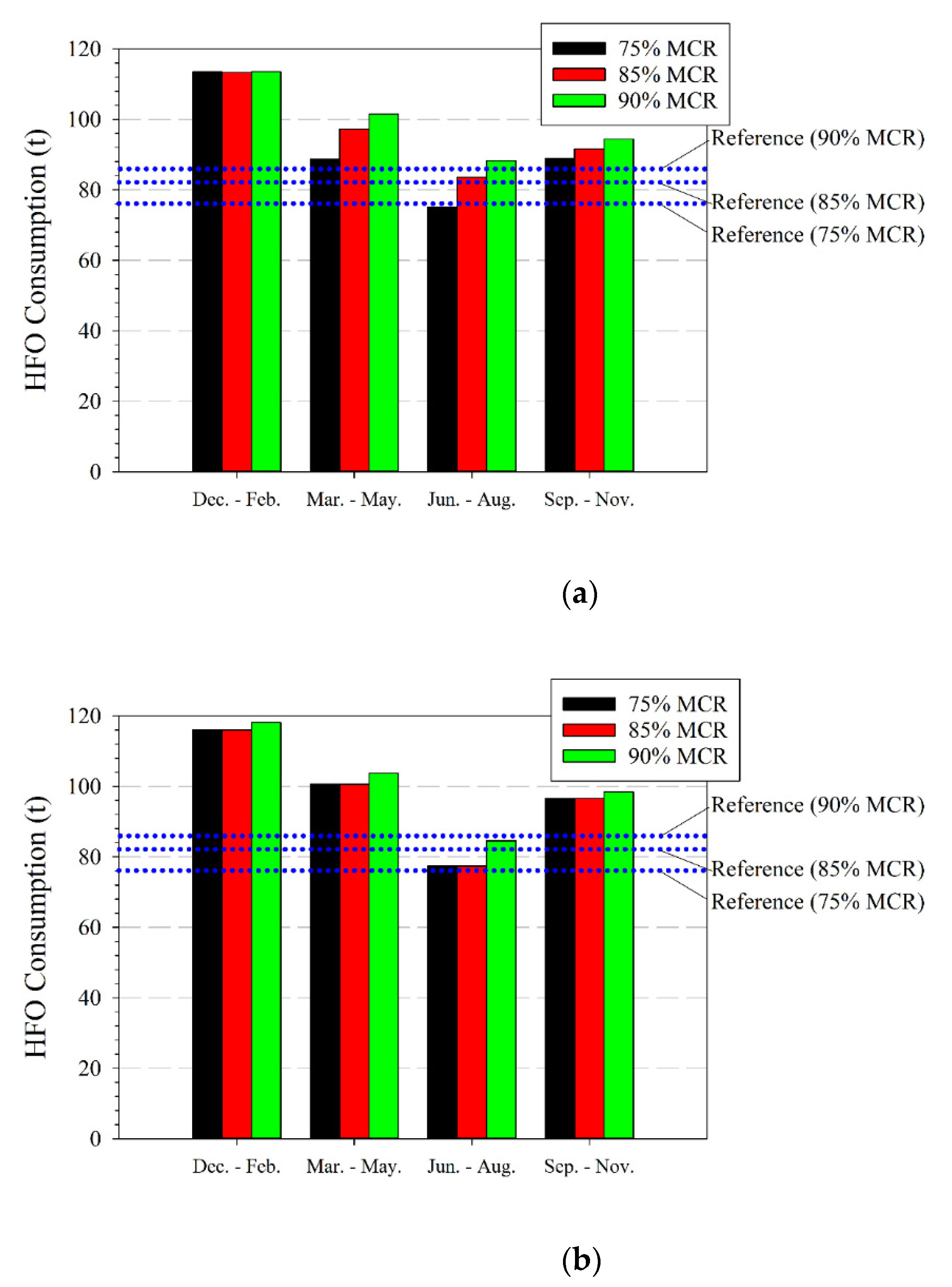
5. Emission and Fuel Consumption Calculations

Numerous works can be found on this matter. For instance, Gutierrez-Romero et al. [48] valued the impact of ship emissions at ports and proposed alternative energy sources to remove pollutant emissions. An extensive review of methodologies to assess ship emissions can be found in Nunes et al. [49]. Others, such as Trozzi [50], for instance, analyzed the world fleet to value emissions and divide each emission by the activities of ships, giving a load of MCR of main and auxiliary engines for different ship activities. Emissions can be determined as:

$$E=t·P·LF·EF,$$

(6)

where $t$ is the running time in hours, $P$ is the power installed in kilowatts, $LF$ is the load factor in percentage of the machinery, and $EF$ is the emission factor per pollutant in kilograms per kilowatt.

The emission factors considered for calculation are as follows: CO₂ 3200 gr/kg of fuel; SO₂ 21 gr/kg of fuel, NO_x 75 gr/kg of fuel; and 25 gr/kg of fuel for particulates.

Table 9. Pollutant emissions and heavy fuel oil (HFO) consumption per season, per Load Condition and, per MCR considered in a voyage.

LC	MCR	75%				85%				90%
	Season	1	2	3	4	1	2	3	4	1	2	3	4
1	CO2 (t)	363.9	284.4	240.9	285.2	363.3	311.5	267.9	293.6	364.0	325.4	283.1	302.8
	SO2 (t)	2.4	1.9	1.6	1.9	2.4	2.0	1.8	1.9	2.4	2.1	1.9	2.0
	NOx (t)	8.5	6.7	5.6	6.7	8.5	7.3	6.3	6.9	8.5	7.6	6.6	7.1
	PMx (t)	2.8	2.2	1.9	2.2	2.8	2.4	2.1	2.3	2.8	2.5	2.2	2.3
	HFO (t)	113.5	88.7	75.1	89.0	113.3	97.2	83.6	91.6	113.5	101.5	88.3	94.4
2	CO2 (t)	371.9	322.5	248.2	309.7	378.8	332.6	271.2	315.4	384.6	335.7	285.0	327.1
	SO2 (t)	2.4	2.1	1.6	2.0	2.5	2.2	1.8	2.1	2.5	2.2	1.9	2.1
	NOx (t)	8.7	7.5	5.8	7.2	8.9	7.8	6.3	7.4	9.0	7.9	6.7	7.7
	PMx (t)	2.9	2.5	1.9	2.4	2.9	2.6	2.1	2.4	3.0	2.6	2.2	2.5
	HFO (t)	116.0	100.6	77.4	96.6	118.1	103.7	84.6	98.4	120.0	104.7	88.9	102.0
B	CO2 (t)	243.4				264.1				275.9
	SO2 (t)	1.6				1.7				1.8
	NOx (t)	5.7				6.2				6.5
	PMx (t)	1.9				2.0				2.1
	HFO (t)	75.9				82.4				86.0

LC = Load Condition. Season: 1 = December to February; 2 = March to May; 3 = June to August; 4 = September to November. B = Base case. Source: Own elaboration.

shows the values of pollutant and heavy fuel oil (HFO) consumption in a voyage, per load condition, per MCR, and per season considered. It is assumed that the consumption of the main engine ranges from 180 to 182 gr/kW·h. The base case refers to the situation in which no added resistance is considered. We assumed that navigation times in both conditions are equal for calm waters.

As noted in Table 9, the highest pollutant emissions and HFO consumption are achieved in Load Condition 2. Under this condition, in December to February, where the weather conditions are the worst, if a nominal case (75% of MCR) is analyzed, the total values increase by approximately up to 50% compared with the base case. In the June to August season, similar values of emissions are obtained compared with base case, because the weather conditions are significantly better. The greater the MCR, the more consumption and emissions are obtained; however, time loss is reduced. Therefore, the shipowner should determine if the increase in fuel consumption is less harmful than the time loss per voyage. In this sense, a freight throughput study is performed below to provide a complete view of the influence of environmental conditions in ship navigation.

Figure 17 and Figure 18 show the CO₂ emissions and HFO consumption. HFO consumption and pollutant emissions increase compared with the base case in the most cases and proposed load conditions. Winter season (December to February) shows an important increase of pollutant emissions and fuel consumption, up to 53% in the case of 75% of MCR. The ship operation during the summer season (June to August) is the least harmful to the environment.

6. Assessment of Freight Loss Due to the Effect of Added Resistance

In liner shipping, speed losses have significant economic impact as shipping companies are under pressure to maintain service level agreement with their cargo clients [51,52].

A sailing speed decision mainly depends on the vessel schedule and it is a challenging problem due to the uncertainties imposed in maritime logistics such as stochastic port times and weather conditions [53]. Focusing on weather conditions, wave and wind affect journey times and the routing decisions [54] as pointed out in the previous sections. In reality, certain routes may encounter harsher weather conditions than others and speed losses need to be considered to assess the performance of the ship in the service route. Thus, knowing speed losses and the associated loss on freight throughput is crucial for liner shipping companies to take optimal decisions on ship management during the voyage.

The navigation times presented in Table 8 have a direct impact on the freight throughput of the ship. An estimation of freight losses was carried out considering 355 operational days per year, a ship with 1775 linear meters of cargo capacity, three values of MCR, two load conditions and four seasons. Moreover, a cargo interchange profile between the three ports was necessary to define. Then, the total freight associated with the round-trip voyage of Barcelona-Genoa-Livorno-Barcelona can be obtained.

Table 10. Associated freight per port and per round-trip voyage.

Ports	Linear Meters Capacity (%)	Linear Meters Capacity (m)
Cargo from Barcelona to Genoa	40	710
Cargo from Barcelona to Livorno	60	1065
Cargo from Genoa to Livorno	20	355
Cargo from Genoa to Barcelona	20	355
Cargo from Livorno to Barcelona	80	1420
Total freight (linear meters)		3905

Source: Own elaboration.

summarizes the interchange of cargo between ports.

Table 11. Estimation of freight loss for Load Condition 1.

MCR (%)		75		85		90
Item		CW	SC	CW	SC	CW	SC
Total time per round-trip voyage (h)	December–February	62.49	86.48	60.41	77.50	59.79	73.75
	March–May		70.64		68.45		67.42
	June–August		61.98		60.82		60.48
	September–November		70.81		65.32		63.70
Number of round-trip voyages per season	December–February	34	24	35	27	35	28
	March–May		30		31		31
	June–August		34		35		35
	September–November		30		32		33
Number of round-trip voyages per year		136	118	140	125	140	127
Maximum freight per season (thousand linear meters)	December–February	132.8	93.7	136.7	105.4	136.7	109.3
	March–May		117.2		121.1		121.1
	June–August		132.8		136.7		136.7
	September–November		117.2		125.0		128.9
Maximum freight per year (thousand linear meters)		531.2	460.9	546.8	488.2	546.8	496.0
Freight loss (% linear meters)			−13.24		−10.71		−9.29

CW: Calm Water; SC: Sea Condition. Source: Own elaboration.

and

Table 12. Estimation of freight loss for Load Condition 2.

MCR (%)		75		85		90
Item		CW	SC	CW	SC	CW	SC
Total time per round-trip voyage (h)	December–February	62.49	88.07	60.41	80.20	59.79	77.13
	March–May		78.23		72.13		69.10
	June–August		63.43		61.40		60.78
	September–November		75.68		69.12		67.70
Number of round-trip voyages per season	December–February	34	24	35	26	35	27
	Mach–May		27		29		30
	June–August		33		34		35
	September–November		28		30		31
Number of round-trip voyages per year		136	112	140	119	140	123
Maximum freight per season(thousand linear meters)	December–February	132.8	93.7	136.7	101.5	136.7	105.4
	March–May		105.4		113.2		117.2
	June–August		128.9		132.8		136.7
	September–November		109.3		117.2		121.1
Maximum freight per year (thousand linear meters)		531.2	437.3	546.8	464.7	546.8	480.4
Freight loss (% linear meters)			−17.65		−15.00		−12.14

CW: Calm Water; SC: Sea Condition. Source: Own elaboration.

show the results of the estimation of freight loss per load condition, per season, and per considered MCR. Times at port in Genoa, Livorno and Barcelona are: 3, 4, and 7 h, respectively. Both tables show the worst condition for the shipowner, which is to navigate during each season in the weather conditions prevailing in each route point and then, with the most likely added resistance associated.

For Load Condition 1, the highest loss would be registered at MCR 75% because the ship would lose 13.24% of its freight with respect to calm waters. In terms of round-trip voyages, the ship would lose 18 round-trip voyages.

For Load Condition 2, the highest loss would also be registered at MCR 75% because the ship would lose 17.65% of its freight with respect to calm waters. In terms of round-trip voyages, the ship would lose 24 round-trip voyages. As expected, the losses in Load Condition 2 are higher than those in Load Condition 1 because the ship navigates with higher displacement.

7. Discussion of Results

In the previous sections, the added ship resistance has been analyzed and it reveals an important impact on the following different aspects: ship velocity, emissions and freight throughput.

The added resistance in irregular waves significantly increases the total ship resistance leading to ship speed loss for the considered route. It becomes up to 10 times higher than wind added resistance in some cases. Added resistance in irregular waves sometimes contributes to the same values as bare hull resistance in some route points. This is especially so in that season and areas where the environmental conditions are rough (Gulf of Lion and Balearian Sea, in December to February season). Therefore, the importance of added resistance on ship navigation is confirmed, as expected. This component of total resistance is influenced by ship load condition, too. An increase in displacement shows higher speed losses if load conditions are compared, as can be deduced from Table 8.

The assumed hypotheses do not consider the change of ship course, the sudden increase of power regime or other things regarding human decisions when ships face the worst conditions. These actions lead a ship to reduce or increase the values of speed loss in a voyage.

Regarding the speed and time losses, they are less influenced by added resistance when the engine regime is higher. Even in this case, the speed loss achieved becomes greater than 10 knots in some cases with respect to 75% of MCR in some route points in the season December to February. Other times, no speed losses are found, when the regime is up to 90% of MCR and the ship sails in the season June to August. Throughout the year, the time losses range between less than 1 h and 26 h approximately (see Table 8).

Speed losses have a direct impact on the freight throughput because they reduce the number of round-trip voyages that the ship can make per operational year. In Load Condition 1, the vessel sailing in calm waters at 90% of MCR could make 140 round-trip voyages; however, with added resistance, the ship could have a loss of 13 round-trip voyages. The loss is equivalent to a loss of 9.29% of freight in terms of linear meters capacity. In Load Condition 2, the highest number of round-trip voyages would be reached at 90% of MCR with 140; however, with added resistance, the ship would lose 17 round-trip voyages. The reduction in the number of round-trip voyages per year is equivalent to a loss of 12.14% of the maximum freight throughput of the ship in the analyzed route.

In relation to emissions and consumption, the increase due to added resistance is clear. The procedure for $f_w$ calculation [20] takes the reference value of 75% of the MCR. If the emissions or the consumption are compared against the base case (calm waters), the increase in emissions is noticeable. The emissions and consumption grow in the range of 31% to 53% in the December to February season if compared with calm water. No differences are found between engine regimes in this season. The gap for different MCRs becomes remarkable for the rest of the seasons.

From an economic point of view, the impact could be great because speed loss increases up to 26 h per voyage in the December to February season. Therefore, in the worst scenario, the ship could lose up to 17.65% of its maximum freight per operational year.

8. Conclusions

The impact of weather on ship navigation is important, and it has been reported in lots of previous studies. Along a whole route, speed losses should be studied anyway because the influence for a given exploitation period of a ship might cause significant freight losses. Commonly, the loss will be greater as the sailing distance per round-trip voyage increases, and it is directly dependent on season.

The importance of ship conditions in added resistance makes this issue a key in the study of added resistance from the results obtained. The contribution of added resistance could make it less feasible from an economic point of view for specific routes in which the weather conditions are usually rough, as can be noted from the analysis performed. The December to February season revealed this conclusion.

The environmental impact of added resistance is clear. Therefore, the questions are the following: do higher velocities contribute to fewer pollutants? Do lower velocities and engine regimes contribute to less pollution? On the one hand, higher velocities are achieved with higher engine regimes, but the consumption could be higher, with more pollutant emissions. On the other hand, the lower velocities require more navigation time in which the ship is emitting polluting gases.

The results show that the freight throughput of a ship decreases because a ship can make fewer round-trip voyages per operational year. In conclusion, in all cases, the emissions increase. This fact should be accounted for by the environmental index of future ships, in an effort to achieve better performance of ship navigation in rough weather conditions.

References

1. Lloyd, A.R.J.M. Ship performance in rough weather. J. Navig. 1978, 31, 93–103. [Google Scholar] [CrossRef]
2. Szlapczynska, J. Multi-objective weather routing with customised criteria and constraints. J. Navig. 2015, 68, 338–354. [Google Scholar] [CrossRef] [Green Version]
3. Journée, J.M.J.; Meijers, J.H.C. Ship Routering for Optimum Performance. Trans. Inst. Mar. Eng. 1980, 92, C56. Available online: http://resolver.tudelft.nl/uuid:805c45f7-bbc0-4baa-802d-637871416490 (accessed on 5 May 2021).
4. Wilson, P.A. A review of the methods of calculation of added resistance for ships in a seaway. J. Wind Eng. Ind. Aerodyn. 1985, 20, 187–199. [Google Scholar] [CrossRef]
5. Lu, R.; Turan, O.; Boulougouris, E. Voyage optimisation: Prediction of ship specific fuel consumption for energy efficient shipping. In Proceedings of the 3rd International Conference on Technologies, Operations, Logistics and Modelling for Low Carbon Shipping, London, UK, 9–11 September 2013. [Google Scholar]
6. Prpić-Oršić, J.; Faltinsen, O. Estimation of ship speed loss and associated CO2 emissions in a seaway. Ocean Eng. 2012, 44, 1–10. [Google Scholar] [CrossRef]
7. Prpić-Oršić, J.; Roberto, V.; Guedes Soares, C.; Faltinsen, O. Influence of ship routes on fuel consumption and CO2 emission. In Proceedings of the 2nd Maritime Technology and Engineering Conference— MARTECH 2014, Lisbon, Portugal, 15–17 October 2014; pp. 857–864. [Google Scholar]
8. Vettor, R.; Prpić-Oršić, J.; Guedes Soares, C. Impact of wind loads on long -terms fuel consumption and emission in trans-oceanic shipping. Brodogradnja 2018, 69, 15–28. [Google Scholar] [CrossRef]
9. Isherwood, R.M. Wind Resistance of Merchant Ships. R. Inst. Nav. Archit. 1972, 115, 327–338. [Google Scholar]
10. Fujiwara, T.; Ueno, M.; Ikeda, Y. A new estimation method of wind forces and moment acting on ships on the basis of physical component models. J. Jpn. Soc. Nav. Archit. Ocean Eng. 2005, 2, 243–255. [Google Scholar] [CrossRef] [Green Version]
11. Degiuli, N.; Ćatipović, I.; Martić, I.; Werner, A.; Čorić, V. Increase of ship fuel consumption due to the added resistance in waves. J. Sustain. Dev. Energy Water Environ. Syst. 2017, 5, 1–14. [Google Scholar] [CrossRef] [Green Version]
12. Kobayashi, H.; Kume, K.; Orihara, H.; Ikebuchi, T.; Aoki, I.; Yoshida, R.; Yoshida, H.; Ryu, T.; Arai, Y.; Katagiri, K.; et al. Parametric study of added resistance and ship motion in head waves through RANS: Calculation guideline. Appl. Ocean Res. 2021, 110, 102573. [Google Scholar] [CrossRef]
13. Shivachev, E.; Khorasanchi, M.; Day, S.; Turan, O. Impact of trim on added resistance of KRISO container ship (KCS) in head waves: An experimental and numerical study. Ocean Eng. 2020, 211, 107594. [Google Scholar] [CrossRef]
14. Lang, X.; Mao, W. A semi-empirical model for ship speed loss prediction at head sea and it validation by full-scale measurements. Ocean Eng. 2020, 209, 107494. [Google Scholar] [CrossRef]
15. Li, X.; Sun, B.; Zhao, Q.; Li, Y.; Shen, Z.; Du, W.; Xu, N. Model of speed optimization of oil tanker with irregular winds and waves for given route. Ocean Eng. 2018, 164, 628–639. [Google Scholar] [CrossRef]
16. Taskar, B.; Andersen, P. Comparison of added resistance methods using digital twin and full-scale data. Ocean Eng. 2021, 229, 108710. [Google Scholar] [CrossRef]
17. Saettone, S.; Taskar, B.; Steen, S.; Andersen, P. Experimental measurements of propulsive factors in following and head waves. Appl. Ocean Res. 2021, 111, 102639. [Google Scholar] [CrossRef]
18. Zis, T.; Psaraftis, H.N.; Ding, L. Ship weather routing: A taxonomy and survey. Ocean Eng. 2020, 213, 107697. [Google Scholar] [CrossRef]
19. Stopford, M. Maritime Economics, 3rd ed.; Routledge: Oxfordshire, UK, 2009. [Google Scholar]
20. Recommended procedures and guidelines. Calculation of the weather factor fw for decrease of ship speed in wind and waves. 7.5-02-07-02.8. In Proceedings of the ITTC International Towing Tank Conference, Zürich, Switzerland, 5–9 November 2018.
21. Compass Ingeniería y Sistemas. Tdyn Theory Manual. Available online: http://www.compassis.com/downloads/Manuals/Tdyn_Theory_Manual.pdf (accessed on 20 January 2020).
22. García-Espinosa, J.; Serván-Camas, B. A non-linear finite element method on unstructured meshes for added resistance in waves. Ships Offshore Struct. 2019, 14, 153–164. [Google Scholar] [CrossRef]
23. Nadukandi, P.; Serván-Camas, B.; Becker, P.A.; García-Espinosa, J. Seakeeping with the semi-lagrangian particle finite element method. Comput. Part. Mech. 2017, 4, 321–329. [Google Scholar] [CrossRef] [Green Version]
24. Colom-Cobb, J.; Garcia-Espinosa, J.; Servan-Camas, B.; Nadukandi, P. A second-order semi-Lagrangian particle finite element method for fluid flows. Comput. Part. Mech. 2020, 7, 3–18. [Google Scholar] [CrossRef] [Green Version]
25. Eurostat. Maritime Transport Statistics—Short Sea Shipping of Goods. Available online: https://ec.europa.eu/eurostat/statistics-explained/index.php?title=Maritime_transport_statistics_-_short_sea_shipping_of_goods (accessed on 29 June 2020).
26. De Osés, F.X.M.; Castells, M. Heavy weather in european short sea shipping: Its influence on selected routes. J. Nav. 2008, 61, 165–176. [Google Scholar] [CrossRef]
27. ECSA (European Community Shipowners’ Associations). Short Sea Shipping. The Full Potential Yet to Be Unleashed; ECSA: Brussels, Belgium, 2016. [Google Scholar]
28. ESPO (European Sea Ports Organisation). Annual Report European Sea Ports Organisation 2018–2019; ESPO: Brussels, Belgium, 2019. [Google Scholar]
29. Puertos del Estado. Oceanography. Available online: http://www.puertos.es/en-us/oceanografia/Pages/portus.aspx (accessed on 15 January 2020).
30. AEMET (Agencia Estatal de Meteorología). Available online: http://www.aemet.es/es/idi/prediccion/meteorologia_maritima (accessed on 25 March 2021).
31. The Wamdi Group. The WAM model—A third generation ocean wave prediction model. J. Phys. Ocean. 1988, 18, 1775–1810. [Google Scholar] [CrossRef] [Green Version]
32. Tolman, H.L. User Manual and System Documentation of WAVEWATCH III Version 4.18; NOAA/NWS/NCEP/MMAB Technical Note, 316; NOAA: College Park, MD, USA; NWS: College Park, MD, USA; NCEP: College Park, MD, USA; MMAB: College Park, MD, USA, 2014; p. 194. [Google Scholar]
33. Bengtsson, L.; Andrae, U.; Asplien, T.; Batrak, Y.; Calvo, J.; de Roy, W.; Gleeson, E.; Hansen-Sass, B.; Mariken, H.; Hortal, M.; et al. The Harmonie–Arome model configuration in the Aladin–Hirlam NWP system. Mon. Weather Rev. 2017, 145, 1919–1935. [Google Scholar] [CrossRef]
34. García-Espinosa, J.; Oñate, E. An unstructured finite element solver for ship hydrodynamics problems. J. Appl. Mech. 2003, 70, 18–26. [Google Scholar] [CrossRef]
35. Menter, F.R. Two-equation eddy-viscosity turbulence models for engineering applications. Am. Inst. Aeronaut. Astronaut. J. 1994, 32, 1598–1605. [Google Scholar] [CrossRef] [Green Version]
36. Wilcox, D.C. Turbulence Modelling for CFD; DCW Industries: La Cañada, CA, USA, 2002. [Google Scholar]
37. Holtrop, J.A.; Mennen, G.G.J. An approximate power prediction method. Int. Shipbuild. Prog. 1982, 29, 166–170. [Google Scholar] [CrossRef]
38. Holtrop, J.A. Statistical reanalysis of resistance and propulsion data. Int. Shipbuild. Prog. 1984, 31, 272–276. [Google Scholar]
39. Fung, S.C.; Leibman, L. Revised speed-dependent powering predictions for high-speed transom stern hull forms. In Proceedings of the FAST ’95: Third International Conference on Fast Sea Transportation, Lübeck-Travemünde, Germany, 25–27 September 1995. [Google Scholar]
40. IMO (International Maritime Organisation). Interim Guidelines for the Calculation of the Coefficient fw for Decrease in Ship Speed in a Representative Sea Condition for Trial Use; IMO Resolution MEPC.1/Circ.796; IMO: London, UK, 2012. [Google Scholar]
41. Compass Ingeniería y Sistemas. SeaFEM Theory Manual. Available online: http://www.compassis.com/downloads/Manuals/SeaFEM_Theory_Manual.pdf (accessed on 10 February 2020).
42. Janssen, W.D.; Blocken, B.; Wan Wijhe, H.J. CFD simulations of wind loads on a container ship: Validation and impact of geometrical simplifications. J. Wind Eng. Ind. Aerodyn. 2017, 166, 106–116. [Google Scholar] [CrossRef] [Green Version]
43. Faltinsen, O.M.; Minsaas, K.J.; Liapis, N.; Skjørdal, S.O. Prediction of resistance and propulsion of a ship in a seaway. In Proceedings of the 13th Symposium on Naval Hydrodynamics, Tokyo, Japan, 6–10 October 1980. [Google Scholar]
44. Barnitsas, M.M.; Ray, D.; Kinley, P. Kt, Kq and Efficiency Curves for the Wageningen B-Series Propellers; Report 237; University of Michigan-Department of Naval Architecture and Marine Engineering: An Arbor, MI, USA, 1981. [Google Scholar]
45. Recommended Procedures and Guidelines; Preparation, Conduct and Analisys of Speed/Power Trials. 7.5-04-01-01.1; ITTC: Zürich, Switzerland, 2017.
46. Taskar, B.; Koosup, K.; Sverre, Y.; Steen, S.; Pedersen, E. The effect of waves on engine-propeller dynamics and propulsion performance of ships. Ocean Eng. 2016, 122, 262–277. [Google Scholar] [CrossRef] [Green Version]
47. IMO (International Maritime Organisation). Guidelines on the Method of Calculation of the Attained Energy Efficiency Design Index for New Ships; IMO Resolution MEPC. 254 (67); IMO: London, UK, 2014. [Google Scholar]
48. Gutiérrez-Romero, J.E.; Esteve-Pérez, J.; Zamora-Parra, B. Implementing onshore power supply from renewable energy sources for requirements of ships at berth. Appl. Energy 2019, 255, 113883. [Google Scholar] [CrossRef]
49. Nunes, R.A.O.; Alvim-Ferraz, M.C.M.; Martins, F.G.; Sousa, S.I.V. The activity-based methodology to assess ship emissions—A review. Environ. Pollut. 2017, 231, 87–103. [Google Scholar] [CrossRef] [PubMed]
50. Trozzi, C. Emission estimate methodology for maritime navigation. In Proceedings of the 19th Annual International Emission Inventory Conference. Informing Emerging Issues, San Antonio, TX, USA, 27–30 September 2010. [Google Scholar]
51. Lee, C.Y.; Lee, H.L.; Zhang, J. The impact of slow ocean steaming on delivery reliability and fuel consumption. Transp. Res. Part E 2015, 76, 176–190. [Google Scholar] [CrossRef]
52. Parthibaraj, C.S.; Subramanian, N.; Palaniappan, P.L.K.; Lai, K. Sustainable decision model for liner shipping industry. Comput. Oper. Res. 2016, 89, 213–229. [Google Scholar] [CrossRef]
53. Lee, H.; Aydin, N.; Choi, Y.; Lekhavat, S.; Irani, Z. A decision support system for vessel speed decision in maritime logistics using weather archive big data. Comput. Oper. Res. 2015, 98, 330–342. [Google Scholar] [CrossRef]
54. Kontovas, C.A. The green ship routing and scheduling problem (GSRSP): A conceptual approach. Transp. Res. Part D 2014, 31, 61–69. [Google Scholar] [CrossRef]
Figure 1. Methodology to value the increase in ship emissions in real operational conditions. Source: own elaboration adapted from International Towing Tank Conference (ITTC) guidelines [20].
Jmse 10 00088 g001
Figure 2. Route selected for calculation (Barcelona–Genoa–Livorno–Barcelona). The numbers in the Figure correspond with each analyzed route point, described in Annex A. Source: Own elaboration.
Jmse 10 00088 g002
Figure 3. General view of the control volume used for computational fluid dynamics (CFD) simulations. Source: Own elaboration.
Jmse 10 00088 g003
Figure 4. Mesh dependence analysis for bare hull resistance computations. Source: Own elaboration.
Jmse 10 00088 g004
Figure 5. CFD details of mesh on bare hull resistance computations. Source: Own elaboration.
Jmse 10 00088 g005
Figure 6. Layout of computational domain used to compute added resistance in waves. Source: Own elaboration.
Jmse 10 00088 g006
Figure 7. Dimensionless added wave resistance versus different wavelengths versus different wave headings in Load Condition 1. (a): Fr = 0.16. (b): Fr = 0.20. (c): Fr = 0.24. Source: Own elaboration.
Jmse 10 00088 g007
Figure 8. Dimensionless added wave resistance versus different wavelengths versus different wave headings in Load Condition 2. (a): Fr = 0.16. (b): Fr = 0.20. (c): Fr = 0.24. Source: Own elaboration.
Jmse 10 00088 g008
Figure 9. Dimensionless added wave resistance versus different wavelengths in head waves. (Right) Load Condition 1. (Left) Load Condition 2. Source: Own elaboration.
Jmse 10 00088 g009
Figure 10. Added wave resistance in irregular waves for two load conditions for Froude number equal to 0.24. (Left) Load Condition 1. (Right) Load Condition 2. Source: Own elaboration.
Jmse 10 00088 g010
Figure 11. Comparison of wind force coefficient obtained by CFD computations and Fujiwara regression method [10]. Source: Own elaboration.
Jmse 10 00088 g011
Figure 12. Streamlines and pressure on ship surfaces for inflow wind conditions of 0 (a) and 30 (b) degrees of relative wind inflow angle. Source: Own elaboration.
Jmse 10 00088 g012
Figure 13. Added wind resistance per each route point and per season considered. Source: Own elaboration.
Jmse 10 00088 g013
Figure 14. Corrected propeller efficiency according to increase in added resistance for a Froude equal to 0.24. (Left) Load Condition 1. (Right) Load Condition 2. Source: Own elaboration.
Jmse 10 00088 g014
Figure 15. Power demand in each route point per load condition and per season. (Left) Load Condition 1. (Right) Load Condition 2. Source: Own elaboration.
Jmse 10 00088 g015
Figure 16. Example of graphical speed loss calculation for one point of route selected in Load Condition 2. Source: Own elaboration.
Jmse 10 00088 g016
Figure 17. CO2 emissions per MCR and per seasons compared with reference lines (blue) of calm waters. (a) Load Condition 1. (b) Load Condition 2. Source: Own elaboration.
Jmse 10 00088 g017
Figure 18. HFO consumption per MCR and per seasons compared with reference lines (blue) of calm waters. (a) Load Condition 1. (b) Load Condition 2. Source: Own elaboration.
Jmse 10 00088 g018