Abstract
In this study, a semi-analytical solution to the dynamic responses of a multilayered transversely isotropic poroelastic seabed under combined wave and current loadings is proposed based on the dynamic stiffness matrix method. This solution is first analytically validated with a single-layered and a two-layered isotropic seabed and then verified against previous experimental results. After that, parametric studies are carried out to probe the effects of the soil’s anisotropic characteristics and the effects of ocean waves and currents on the dynamic responses and the maximum liquefaction depth. The results show that the dynamic responses of a transversely isotropic seabed are more sensitive to the ratio of the soil’s vertical Young’s modulus to horizontal Young’s modulus (Ev/Eh) and the ratio of the vertical shear modulus to Ev (Gv/Ev) than to the vertical-to-horizontal ratio of the permeability coefficient (Kv/Kh). A lower degree of quasi-saturation, higher porosity, a shorter wave period, and a following current all result in a greater maximum liquefaction depth. Moreover, it is revealed that the maximum liquefaction depth of a transversely isotropic seabed would be underestimated under the isotropic assumption. Furthermore, unlike the behavior of an isotropic seabed, the transversely isotropic seabed tends to liquefy when fully saturated in nonlinear waves. This result supplements and reinforces the conclusions determined in previous studies. This work affirms that it is necessary for offshore engineering to consider the transversely isotropic characteristics of the seabed for bottom-fixed and subsea offshore structures.
1. Introduction
With the rapid development of technologies, marine resources are being exploited on a large scale. A great number of onshore and offshore structures have been built in the new century, such as cross-sea bridges, submarine pipelines, subsea oil and gas production systems, submarine tunnels, and offshore wind turbines. Offshore structures mainly suffer from wind, wave, current, and ice loadings, whose characteristics tend to be random and recurrent in nature. These environmental loadings are usually coupled, such as wind-wave interaction, wave-current interaction, and wind-wave-current interaction. When acting on marine structures, the coupled loadings can lead to pipeline disturbance, breakwater subsidence, abutment scour, and corrosion [1,2,3,4], causing a huge loss of property. A number of studies [5,6,7] have proved that the failures of offshore structures are not only attributed to inadequate structural strength but also the instability of the seabed. As waves and/or currents propagate in seawater, a time-varying wave pressure will be generated on the surface of the seabed, thus increasing the excess pore water pressure and decreasing the effective stress of the soil skeleton. When the excess pore water pressure is greater than the effective stress of the soil, liquefaction may occur and subsequently causes engineering structures to fail. Hence, it is necessary to study the dynamic responses of the seabed under wave and/or current loading.
At present, the dynamic responses of the seabed under wave loading have been studied by three main approaches, i.e., analytical derivation, indoor tests, and numerical simulations. The analytical derivation is usually based on the three-dimensional consolidation theory and the early porous elastic solid-fluid system developed by Biot [8,9]. The theory assumed that the seabed was a porous, saturated two-phase medium, of which the soil skeleton and the pore fluid were both compressible and the flow of pore fluid followed Darcy’s law. Hereafter, three simplified and commonly used models were summarized by Zienkiewicz et al. [10], i.e., a quasi-static (QS) model which ignored the acceleration terms of both soil skeleton and pore fluid, a partially dynamic (PD) model which ignored the acceleration term of the soil skeleton, and a fully dynamic (FD) model which considered both acceleration terms. Among them, the QS model has been extensively investigated due to relatively explicit equations, and the accuracy can basically meet the demands of engineering applications. Yamamoto et al. [11] deduced an analytical solution to the dynamic responses of a single-layered isotropic poroelastic seabed under linear regular waves. Madsen [12] and Seymour et al. [13] presented similar solutions, but they considered the hydraulic anisotropy of soil. Yamamoto [14] and Rahman et al. [15] extended Madsen’s QS analytical solution to a stratified seabed and to three dimensions, respectively. In 2007, Liu and Jeng [16] made a breakthrough to propose a semi-analytical solution to a single-layered isotropic poroelastic seabed under random waves. However, some studies [17,18,19,20] have pointed out that the QS model only performs better for sandy soil, and the omitted inertial term played an important role in the dynamic behavior of the seabed. Hence, Jeng et al. [21], Jeng and Rahman [22], and Jeng and Lee [23] derived the governing equations based on the PD model and the FD model and gave analytical solutions to a single-layered isotropic poroelastic seabed under linear regular waves. Ulker et al. [19] compared the dynamic responses and the stabilities of the QS, PD, and FD models, also under linear waves. It was shown that the QS model and the PD model have similar performances and are more conservative than the FD model. Therefore, the FD model was recommended to achieve the least conservative response. In addition to analytical solutions, numerical finite element calculations and laboratory experiments were also conducted by a number of research works [24,25,26,27,28,29], which were in good agreement with analytical results.
Nevertheless, it should be noted that the aforementioned studies have only considered ocean waves, and yet ignored the influence of sea currents which are common in the marine environment. Ye and Jeng [30] initiated the analysis of the dynamic responses of a single-layered isotropic poroelastic seabed under wave and current loadings in two dimensions based on the PD model and discussed the transient liquefaction depth of the seabed, respectively, under a following current and an opposing current. Their conclusions indicated that the current’s influence on the pore pressure should not be neglected, and the maximum liquefaction depth increases under the following current while decreasing under the opposing current. Zhang et al. [31] further compared the seabed’s dynamic responses of coarse sand and fine sand under various wave and current conditions. The comparison showed that the pore pressure of both coarse sand and fine sand seabeds has the tendency to increase when the current and nonlinear waves are taken into account. Liu et al. [32] also adopted the PD model and proposed analytical solutions for seabeds of finite and infinite thicknesses under combined nonlinear wave and current loadings. It was found that the maximum liquefaction depth is 19% greater in the presence of a current.
It is worth mentioning that the seabed was assumed isotropic in the above studies. As a matter of fact, anisotropy of the seabed does exist since marine sediments originate from different compositions, types of accumulation, and stress history. For an anisotropic medium, its constitutive model has 21 independent elastic coefficients [33] that are difficult to experimentally determine. Consequently, a transversely isotropic medium was recommended by the literature to model a porous seabed whose constitutive model consists of only five independent coefficients. Compared with the isotropic assumption, such a model more reasonably describes the actual site conditions. Meanwhile, this model is less complicated in analysis and computation than the fully anisotropic assumption for fewer constants. An analytical solution to a single-layered transversely isotropic poroelastic (TIP) seabed and a semi-analytical solution to a multilayered TIP seabed have been proposed in recent research works [34,35,36,37,38]. However, it should be noted that these works were limited to linear waves only, without accounting for the interaction between waves and current, let alone the nonlinearity of waves. This thereby motivates the present study.
In this paper, a semi-analytical solution to the dynamic responses of a multilayered TIP seabed under combined wave-current loading is developed. The solution is derived based on the well-developed method of the dynamic stiffness matrix in earthquake engineering. This solution is first validated analytically using a single-layered and a two-layered isotropic seabed and then verified with previous experimental results. The parameters of anisotropic soil, waves, and currents are analyzed to probe their effects on the dynamic responses and maximum liquefaction depths of the single-layered TIP and the multilayered TIP seabed.
2. Seawater-Seabed-Bedrock System
A two-dimensional (2D) seawater-seabed-bedrock system subjected to combined wave-current loading is illustrated in Figure 1. The Cartesian coordinate system is adopted where the Z-axis is positive downwards from the mudline and the X-axis is positive along the mudline. The progressive wave is assumed to be periodic with wavelength L and wave height H. The current is assumed uniform with a velocity U0. The seawater overlaying the seabed is considered inviscid, incompressible, and irrotational with a constant depth d. Since the marine sediment is characterized by anisotropy, the seabed in this study is modeled as N-layered stratified soil, and each layer is assumed homogeneous, transversely isotropic, and poroelastic. The interfaces of the soil layers are numbered from z0 at the mudline to zN at the bedrock, and the thickness of layer j is hj = zj − zj−1. Besides, the bedrock is regarded as an impermeable, rigid, and elastic half-space.
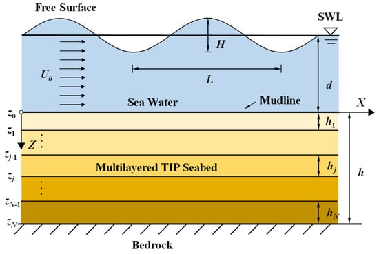
Figure 1.
Sketch of a multilayered TIP seabed under a wave-current interaction.
2.1. Governing Equations
The seabed usually comprises three phases: solid, liquid, and gas. Because of the overlaying seawater, the saturation of the seabed is sufficiently high so that the gas phase is embedded in the liquid phase in the form of bubbles. In an early work, Sparks [39] and Barden [40] found that the air bubbles are occluded and the pressure in gas and liquid is quite close. This implied that the mixture of gas and liquid phases can be considered as an equivalent homogeneous pore fluid that completely fills the pores of the soil. Consequently, Chang and Duncan [41] developed a theory of ‘homogenized pore fluid’. This theory is adopted in this study to model the reduced two-phase medium of soil where both the homogenized pore fluid, hereinafter called the pore fluid for short, and the solid phase, which is also called the soil skeleton, are assumed compressible.
Based on the FD formulation for a two-phase medium [10], the overall equilibrium equations for a unit total volume are expressed as follows. The inertial forces associated with the pore fluid and the soil skeleton are involved in these equations.
where σxx, σzz, τxz are the total stress tensors of the two-phase medium (tensile stress is positive); p is the pore pressure; g is the gravitational acceleration; ρ = (1 − n) ρs + nρf is the equivalent density of the two-phase medium, in which ρs is the density of the soil skeleton, ρf is the density of the pore fluid, and n is the soil porosity; ux (uz) is the displacement component of the soil skeleton in X (Z) direction; wx (wz) is the displacement of the pore fluid relative to ux (uz) in X (Z) direction; and Kh and Kv are the horizontal and vertical soil permeability coefficients in Darcy’s law.
In the early three-dimensional (3D) constitutive model by Biot [9,42], the TIP medium and material coefficients were determined. For the 2D TIP medium in Figure 1, taking Z-axis as the symmetry axis, the constitutive model can be reduced to:
where , , are the effective stresses controlling the deformation of the soil skeleton; exx, ezz, and exz are the strain tensors of the TIP medium, in which exx = ux,x, ezz = uz,z, exz = (ux,z+uz,x)/2; ξ = ▽·w represents the volumetric strain in the fluid; and M11, M12, M13, and M33, M44 are the aforementioned five elastic coefficients and M, α1, α3 are their derived parameters.
where Eh, Ev and νh, νv denote Young’s moduli and Poison’s ratios in horizontal (X) and vertical (Z) directions, respectively; Gv is the shear modulus in a vertical direction; Ks is the bulk modulus of the soil skeleton; and Kf is the bulk modulus of the pore fluid, dependent on the bulk modulus of water Kw, the absolute pore fluid pressure Pw0, and the degree of saturation Sr in the following formula [43]:
where Pw0 is usually taken as 2 × 10⁹ Pa [11]. It should be noted again that Equation (17) is primarily applicable to a poroelastic medium of high saturation exceeding 0.9 [44]. When the seabed is fully saturated (i.e., Sr = 1), Kf = Kw.
2.2. Wave-Current Interaction
Hsu et al. [45] derived a third-order approximation of the velocity potential for nonlinear wave-current interactions based on the perturbation technique. The corresponding third-order hydrodynamic pressure acting on a flat seabed (psb) was subsequently obtained by Zhang et al. [31], as follows:
where k = 2π/L is wave number, ω = 2π/T is wave circular frequency, T is wave period, and ω1 is the circular frequency for the well-known linear dispersion for Airy waves.
The nonlinear dispersion relation is given by:
where ω0 and ω2 are both intermediate frequencies, expressed as:
2.3. Boundary Conditions
To determine the pore pressure and the stress components of a TIP medium, some typical boundary conditions should be applied to the governing equations.
At mudline z = 0, the vertical effective normal stress and shear stress of the soil are zero, since the extremely small frictional stress at the seawater–seabed interface can be ignored [12]. Besides, the soil pore pressure there is equal to the hydrodynamic pressure defined in Equation (18).
As at z = h, the bedrock is assumed rigid and impermeable and the displacements of the soil skeleton and the vertical flow are zero, i.e.,
3. Semi-Analytical Solution
3.1. General Solution to a TIP Layer
Since the acting hydrodynamic pressure of Equation (18) is regarded as a superposition of three harmonic components, the horizontal and vertical displacements of the soil skeleton ux and uz, as well as the pore pressure p, can be similarly written as:
where pm is the amplitude of each harmonic hydrodynamic component already defined in Equation (18) and i is the imaginary unit. In Equations (1)–(4), if the body force ρfg is neglected like Chen et al. [20], wx and wz can be eliminated. It follows that the substitution of Equations (5)–(8) and Equation (25) into Equations (1)–(4) results in three reorganized formulas:
where m = 1,2,3, fqm (q = 1, …, 6) and βzm are parameters listed in Appendix A.
Now, introducing the potential function Φm to Equations (26) and (28), the solution to the three unknowns in Equation (25) can be deduced as follows:
Substituting the above three equations into Equation (27), Equations (26)–(28) can be simplified to:
where rcm (c = 1, …, 4) are illustrated in Appendix B.
Equation (32) is a sixth-order differential equation whose general solution can be solved analytically as the extension of Jeng [35]:
where m = 1,2,3 and ± λlm, given in Appendix C, are eigenvalues of Equation (33). Coefficients Alm and Blm are to be determined by the boundary conditions in Section 2.3.
Substituting Equation (33) back into Equations (29)–(31), we have:
where γlm, ϑlm, χlm, and κlm are the parameters given in Appendix D. Other parameters, such as stress tensors, are subsequently worked out by substituting Equations (34)–(36) into Equations (1)–(4). Therefore, the total dynamic responses of a TIP medium under third-order wave-current loading can be summarized as follows:
Note that when m = 1 and Equations (37)–(42) are normalized by p1, the above solutions will reduce to those given by Li et al. [38], which was derived under linear regular waves.
3.2. Dynamic Stiffness Matrix of TIP Multilayers
To solve the displacement components and the stress tensors of a multilayered TIP seabed, a global dynamic stiffness matrix (DSM) of multilayers is derived. Such a scheme is more straightforward than the so-called dual variable and position method [46], which requires repeated applications of recursive relations between two adjacent layers. Herein, the local DSM of a single layer is first derived (Figure 2). Then, the global DSM of multilayers is formulated by assembling the local DSMs of single layers.
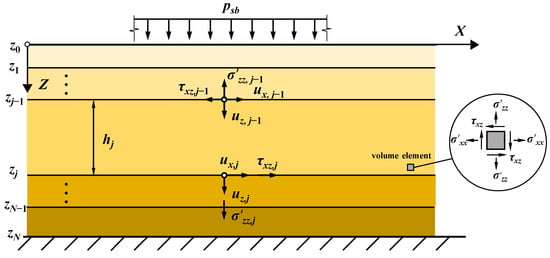
Figure 2.
A multilayered TIP seabed subjected to hydrodynamic pressure.
At depth z, for each order of hydrodynamic pressure (m = 1, 2, 3), we denote the following vectors and matrices:
where vectors Um(z) and Rm(z) essentially synthesized displacement and stress components at z. It follows that Equations (37)–(42) can be reorganized into a matrix form as:
where [Dm] (m = 1,2,3) are 6 × 6 matrices defined in Appendix E. It can be proven that they are non-singular. Eliminating the unknown vector [Am(z), Bm(z)]T in Equation (49), the dynamic relationship between (j − 1)-th and the j-th layer can be deduced as:
where hj = zj − zj−1 is the thickness of the j-th layer. For the sake of simplicity, a similarity transformation on the RHS of Equation (50) is denoted as:
where [] is a block matrix whose submatrices [] (a,b = 1,2) are of dimensions 3 × 3. The superscript j is used to denote the quantities associated with the j-th layer. Then, Equation (50) can be expressed as:
In order to employ the DSM for constructing the relation between forces and displacements, it is necessary to swap the vectors Um(zj) and Rm(zj−1) in Equation (52) to derive the DSM of a singer layer. Besides, it must be realized that the above derivation is within the local coordinate where the positive directions of the stress tensors, such as τxz and , on the top and the bottom faces are opposite (Figure 2). However, the applied external loadings are defined in the global coordinate where the DSMs of all layers are assembled. Hence, for a single layer subjected to external forces, Pm(zj−1) = −Rm(zj−1) and Pm(zj) = Rm(zj) (Figure 3), Equation (52) can be further deduced to:
where [] is the 6 × 6 local DSM whose submatrices [] (a,b = 1,2) are functions of [] (a,b = 1,2), given in Appendix F.
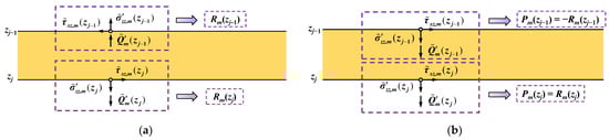
Figure 3.
Positive stress directions in (a) local coordinates and (b) global coordinates.
Therefore, for a multilayered seabed, the linear relationship between its global displacements and external forces can be expressed as:
where [GSm] is the global DSM whose dimensions are (3N + 3) × (3N + 3). On the LHS of Equation (55), external forces Pm(zj) (j = 0, …, N – 1) are known, while Pm(zN) needs to be determined. Pm(zj) (j = 1, …, N – 1) are all zeros while only Pm(z0) is nonzero because the hydrodynamic pressure induced by the wave–current interaction is only exerted on the mudline of z = 0. Now, combining the boundary conditions in Equations (23) and (24), Pm(z0) and Um(zN) can be rewritten in the non-dimensional form as:
Collecting all knowns and unknowns respectively in Equations (55) and (56) leads to:
where the complete matrix form of [Sm] is given in Appendix G. Clearly, the unknown vectors [Um(z0), …,Um(zj), …, Um(zN-1),Pm(zN)]T can be solved by:
Note that [Sm] tends to be singular in high-frequency waves and thick layers due to the existence of positive exponential terms [47]. However, some numerical algorithms, i.e., the singular value decomposition (SVD), are available to solve Equation (58) without recourse to the inverse matrix of [Sm], which is out of the scope of this study. After the unknown vectors in Equation (59) are determined, vector [Am(z), Bm(z)]T in Equation (49) can be solved. Lastly, the desired semi-analytical solution to the dynamic responses (displacements and stresses) in Equations (37)–(42) for a multilayered TIP seabed at any depth z can be determined.
4. Verification of the Semi-Analytical Solution Based on Isotropic Layers
To validate the accuracy of the semi-analytical solution derived in the above section, two particular cases are examined. One is single-layered, and the other is two-layered, but all are assumed isotropic. Li et al. [38] have presented a semi-analytical solution for linear regular waves (m = 1) but without the presence of current. Figure 4 makes a comparison between this solution with the present study. In this figure, the normalized wave-induced soil stresses with respect to the maximum hydrodynamic pressure pmax that acts on the mudline are shown. The corresponding wave conditions and soil properties of the single-layered seabed are listed in Table 1. For the two-layered seabed, except for the shear modulus of the second layer G = 2 × 10⁷ Pa, all parameters are identical to those of the single-layered. In Figure 4, it can be obvious that, in both cases, not only the effective stresses of the soil but also the pore pressures are in very good agreement between the semi-analytical solution by Li et al. [38] and the present study.
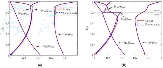
Figure 4.
Comparisons of the vertical stress distributions of (a) a single-layered seabed and (b) a two-layered seabed between Li et al. [38] (solid lines) and present study (dash lines).

Table 1.
Wave conditions and isotropic soil properties [38].
Further, the validation of the present solution is conducted against the experimental results by Qi et al. [48]. The soil and wave conditions in the experiment are given in Table 2. Note that wave number k and wavelength L vary with current velocity U0 due to the Doppler effect. Hence, k and L should be determined by the dispersion relations in Equations (19)–(22). The cases of waves only (U0 = 0), waves with a following current (U0 > 0), and waves with an opposing current (U0 < 0) for different wave periods are considered (Figure 5). This figure illustrates the comparison of vertical distributions of the maximum pore pressure under these wave-current conditions between the experimental results and the present semi-analytical solution. In Figure 5, it is shown that the semi-analytical solution and experimental results basically match well in every case, especially for the case of waves only (U0 = 0). However, the analytical solution tends to be slightly larger than the experimental data under U0 > 0, and slightly smaller under U0 < 0. This phenomenon was reported by Qi et al. [48], but no elaboration was given. It is pointed out herein that the actual profile of U0 in the experiment was not ideally uniform but logarithmic from the still water level to mudline [49]. The vertically averaged current velocity, which was supposed to be an input for the semi-analytical solution, cannot be directly measured, since the depth of the averaged current velocity was unknown. It cannot be determined by an integration until the profile of U0 is shaped. However, shaping a reasonable profile was not an easy task. It demanded multi-point measurement and curve fitting. Hence, the current speed of 0.5 h (e.g., z = 0.25 m), which can be directly measured, has been adopted as the semi-analytical solution’s input [48]. It was somehow greater than the actual averaged current velocity due to the logarithmic profile of U0. In a hydrodynamic sense, when U0 > 0, a greater U0 leads to a smaller wave number k and a greater pore pressure p in the soil. In contrast, when U0 < 0, a greater U0 results in a larger k and a smaller p. Such tendencies are plotted in Figure 6 and Figure 7 using Equations (19)–(22) for T = 12 s, d = 30 m, h = 30 m, and H = 8 m as an example. In Figure 7, it is shown that the normalized first-order hydrodynamic pressure (Equation (18)) by ρfgH/2 decreases with increasing k. This well explains why the analytical solution is slightly larger than the experimental results for U0 > 0 while slightly smaller for U0 < 0.
Table 2.
Wave conditions and isotropic soil properties [48].
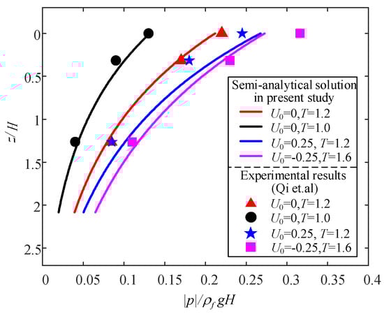
Figure 5.
Comparisons of the vertical distributions of the maximum pore pressure between the experimental results by Qi et al. [48] (markers) and the present semi-analytical solution (dashed line).
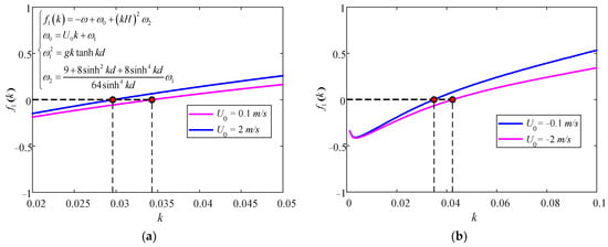
Figure 6.
Wave number k (a) in a following current and (b) in an opposing current.
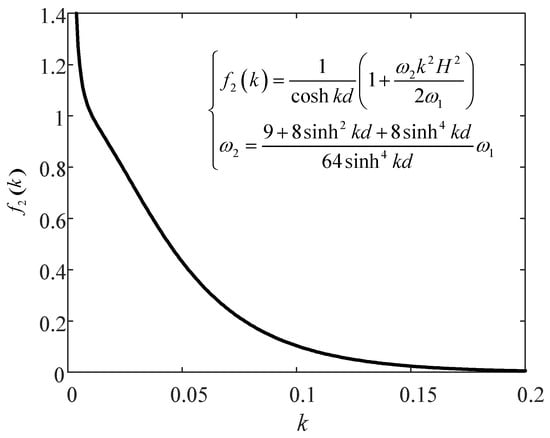
Figure 7.
The normalized first-order pore pressure f2(k), varying with wave number k.
5. Semi-Analytical Solution Applied to TIP Layers and Parametric Study
The dynamic responses and the maximum liquefaction depths of the seabed subjected to a variety of soil, wave, and current conditions are studied in this section. Two patterns of seabeds are considered. One is a single TIP layer with a 30 m thickness, and the other contains three TIP layers of identical thicknesses of 10 m but distinct soil characteristics. The assumed wave and current conditions as well as the soil properties are shown in Table 3.
Table 3.
Wave and current conditions and TIP soil properties.
To validate the use of the third-order hydrodynamic pressure in Equation (18), the wave conditions specified in Table 3 must fall into the category of the Stokes third-order waves. For this, three wave periods (T = 12 s, 15 s, 17 s) are examined. Table 4 presents the corresponding H/gT2 and d/gT2 that are non-dimensional parameters in the well-known chart by Le Méhauté [50] in Figure 8. Obviously, the Stokes third-order wave model is applicable to these three regular waves. Thus, in the presence of a current, it is reasonable to apply Equation (18) to account for the effect of wave-current interactions on hydrodynamic pressure.
Table 4.
Parameters of waves.
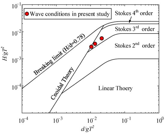
Figure 8.
Limits of validity for various wave theories (Le Méhauté [50]).
The liquefaction criterion proposed by Zen and Yamazaki [51] is employed to study the maximum instantaneous liquefaction depth, i.e.,
where γsat and γw are the saturation unit weight of seabed soil and the unit weight of water, respectively. Equation (60) indicates that when the excess pore pressure −(psb − p) induced by wave--current interactions is no less than the initial vertical effective stress (γsat − γw)z, the soil skeleton will enter a liquefied state.
5.1. Single-Layered Seabed
Figure 9 illustrates the vertical distributions of normalized maximum pore pressure |p|, shear stress |τxz|, and vertical and horizontal effective stress || and || for various vertical-to-horizontal permeability coefficient ratios Kv/Kh, where pmax denotes the maximum hydrodynamic pressure acting on the mudline (z = 0). The horizontal permeability coefficient Kh is fixed with 1 × 10⁻⁴ m/s, and the vertical permeability coefficient Kv varies. In Figure 9, the vertical distributions of |p|, || and || are influenced by Kv/Kh. The larger the ratio, the greater the influence on these three quantities. However, the vertical distribution of |τxz| is hardly affected by Kv/Kh within a range from 0.5 to 100. When Kv/Kh is small (0.5, 1, 2), it has little influence on the vertical distribution of |p|, || and || for z/h > 0.2. Similar results under linear wave conditions were drawn by Li et al. [38].
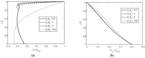
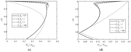
Figure 9.
Vertical distributions of normalized maximum (a) pore pressure, (b) shear stress, (c) vertical effective stress, and (d) horizontal effective stress by varying Kv/Kh.
Figure 10 demonstrates the relationship between the maximum liquefaction depth zmax versus Kv/Kh for various soil and wave parameters. The effects of the degree of saturation Sr, wave period T, soil porosity n, and current velocity U0 on zmax are studied. It can be observed that zmax decreases almost linearly with Kv/Kh. Under the same Kv/Kh, zmax increases with decreasing Sr, increasing n and decreasing T. As for U0, a following current helps to raise the liquefaction depth while an opposing current reduces the liquefaction depth. Particularly, Figure 10a shows that zmax becomes less sensitive to Kv/Kh when Sr gets smaller. Moreover, it illustrates that when Kv/Kh > 1, zmax would be overestimated using an isotropic model (Kv/Kh = 1), and vice versa, underestimated for Kv/Kh < 1.
Figure 10.
Maximum liquefaction depth zmax versus Kv/Kh for various (a) degrees of saturation, (b) wave periods, (c) soil porosities, and (d) current velocities.
The effects of Ev/Eh on the vertical distributions of normalized |p|, |τxz|, || and || are also studied, as shown in Figure 11. Here, Eh = 2.6 × 10⁷ Pa, while Ev varies. Unlike Kv/Kh, Ev/Eh affects not only the vertical distributions of all |p|, ||, and || but also |τxz|. However, with the increase in Ev/Eh (from 0.5 to 2), the normalized |p|, |τxz|, and || at the same depth all basically decrease, while || increases. Meanwhile, the influences of Ev/Eh on the normalized |p|, |τxz|, || and || all decay with the increase in Ev/Eh.
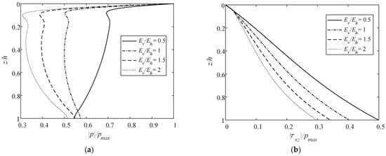
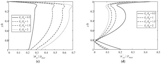
Figure 11.
Vertical distribution of normalized maximum (a) pore pressure, (b) shear stress, (c) vertical effective stress, and (d) horizontal effective stress by varying Ev/Eh.
Figure 12 denotes zmax versus Ev/Eh for various Sr, T, n, and U0. On the contrary to the effect of Kv/Kh, zmax increases with Ev/Eh, showing the tendency of more severe liquefaction. For the same Ev/Eh, zmax increases with decreasing Sr and T but increasing n. Similar to the effect of Kv/Kh, the following current aggravates the liquefaction depth whilst the opposing current alleviates the liquefaction depth. It is obvious that even though |U0| is equal, the direction of the current can lead to varying degrees of change in zmax. Besides, if the seabed is regarded as isotropic, zmax would be underestimated when Ev/Eh > 1 but overestimated when Ev/Eh < 1.
Figure 12.
Maximum liquefaction depth zmax varying with Ev/Eh for various (a) degrees of saturation, (b) wave periods, (c) soil porosities, (d) current velocities.
Figure 13 shows the vertical distributions of normalized |p|, |τxz|, ||, and || for various ratios of vertical shear modulus to vertical Young’s modulus Gv/Ev, where Gv/Ev = 1/2.6 and corresponds to the isotropic case. A fixed value of Ev = 2.6 × 10⁷ Pa is chosen. Similar to Ev/Eh, Gv/Ev changes all vertical distributions of |p|, |τxz|, ||, and ||. Especially, zmax at || = 0 is more significantly affected by Gv/Ev than by Kv/Kh and Ev/Eh, referring to Figure 9d, Figure 11d, and Figure 13d.
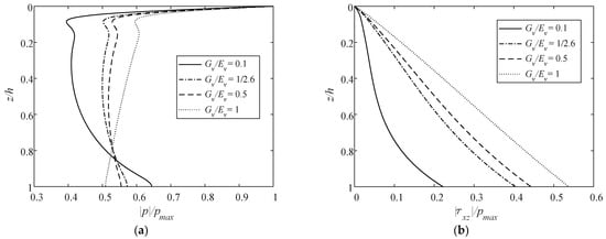
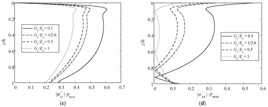
Figure 13.
Vertical distributions of normalized maximum (a) pore pressure, (b) shear stress, (c) vertical effective stress, and (d) horizontal effective stress by varying Gv/Ev.
Figure 14 indicates that for various Sr, T, n, and U0, zmax decreases with growing Gv/Ev. At a given Gv/Ev, zmax increases with decreasing Sr and T but increasing n. Figure 14d shows that zmax under the following current is also greater than under the opposing current. Additionally, assuming an isotropic seabed, zmax would be underestimated when Gv/Ev < 2(1 + v) but overestimated when Gv/Ev > 2(1 + v).
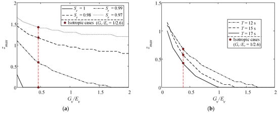
Figure 14.
Maximum liquefaction depth zmax varying with Gv/Ev for various (a) degrees of saturation, (b) wave periods, (c) soil porosities, and (d) current velocities.
From the above discussion, brief conclusions can be drawn. The responses of pore pressure and effective stress are more sensitive to the anisotropic characteristics of Ev/Eh and Gv/Ev than to Kv/Kh. A lower quasi-saturation rate of Sr = 0.97, higher porosity, shorter wave period, and a following current would result in the aggravation of the maximum liquefaction depth. Furthermore, as shown in Figure 10a, Figure 12a, and Figure 14a, for a large Ev/Eh and small Kv/Kh and Gv/Ev, the liquefaction can still happen even if the TIP seabed is fully saturated (Sr = 1). This is different from the conclusions drawn by Rahman [52] that the transient liquefaction does not occur in fully saturated isotropic sediments. Like the soil studied by Rahman [52], the seabed layers in this study are cohesionless because the adopted permeability coefficients fall into the empirically cohesionless range [53]. For example, in Figure 10a, liquefaction occurs when Sr = 1 and Kv/Kh = 0.5, i.e., Kv = 5 × 10⁻⁵ m/s and Kh = 1 × 10⁻⁴ m/s. In Figure 12a and Figure 14a, where Kv and Kh are fixed to 1 × 10⁻⁴ m/s, the liquefaction does occur when Sr = 1. The permeability coefficients in these three figures are categorized by clean sand or clean sand and gravel mixtures which are essentially cohesionless sediments in Table 14.1, according to Terzaghi et al. [53]. Thus, the importance of transverse isotropy is manifested, especially for the liquefaction assessment under wave-current loading.
Similar to the present study, Jeng [35] did not emphasize the role of soil cohesion, although the treated medium was actually cohesionless in terms of permeability coefficients. It also used parameters of Kv/Kh, Ev/Eh, and Gv/Ev to characterize the anisotropic soil. A similar conclusion that liquefaction did not occur in fully saturated (Sr = 1) sediments was determined in Jeng [35]. To dig out the reason for Jeng’s conclusion, which seems contradictory to this study, an elaborate numerical test was conducted, as shown in Table 5. The ratio Ev/Eh from 0.4 to 2.5 is taken as a variable. The analytical solution proposed by Li et al. [38] of an infinite thickness single-layered seabed is adopted. The wave conditions and TIP soil properties by Jeng [35] are shown in Table 6. Table 5 illustrates that an infinite thickness seabed under linear waves only—which is exactly Jeng’s assumption—would not liquefy. However, the calculation results in this study show that liquefaction occurs in nonlinear waves, especially in soil with finite thickness. Among the 16 cases in Table 5, only four cases yield liquefaction. These four cases correspond to the nonlinear wave model and finite thickness. The reasons for liquefaction in nonlinear waves and soil with finite thickness may be summarized as follows: (i) In a nonlinear wave, though the first-order (linear) hydrodynamic pressure is of the largest weight, the second- and third-order terms cannot be neglected, especially in a severe sea state. The greater the hydrodynamic pressure, the greater the possibility for liquefaction. (ii) An infinite seabed tends to dissipate more pore pressure and bear more effective stress than a finite seabed does. An infinite thickness seabed can be considered to consist of two layers of identical properties. The thickness of the upper layer is the same as that of a finite-thickness seabed. Then, the only difference between infinite and finite thickness seabeds lies in the lower layer. One is bedrock while the other is still soil. Therefore, the bedrock of a finite thickness seabed is impermeable, which is not the case in an infinite thickness seabed. This makes an infinite seabed tend to dissipate more pore pressure and bear more effective stress than a finite seabed. The greater the effective soil stress, the lesser the possibility for liquefaction.
Table 5.
Calculated liquefaction results for two wave conditions, two TIP soil properties, and two thicknesses (Sr = 1).
Table 6.
Wave conditions and TIP soil properties by Jeng [35].
5.2. Multilayered Seabed
5.2.1. Effects of Permeability Coefficient
In order to describe the actual site conditions more reasonably, the seabed is further modeled as a three-layered TIP medium. First, the effects of the permeability coefficient on the multilayered seabed are investigated. For the convenience of discussion, the ratio Kv/Kh of each layer is fixed to 2, and the vertical permeability coefficient ratios of three layers Kv1: Kv2: Kv3 vary. Several typical cases are considered, as shown in Figure 15. It is worth noting that the three-layered TIP seabed degrades to the single-layered isotropic one when Kv1: Kv2: Kv3 = 2:2:2 and Kv1: Kv2: Kv3 = 20:20:20. This is because Kho (o = 1, 2, 3), in the former case, is 1 × 10⁻⁴ m/s, but in the latter case is 1 × 10⁻³ m/s, and all Kh and Kv are relative to the typical value 1 × 10⁻⁴ m/s in Table 3. In this section, the soil parameters and wave conditions are still taken from Table 3. They follow the specification in the second footnote of this table.
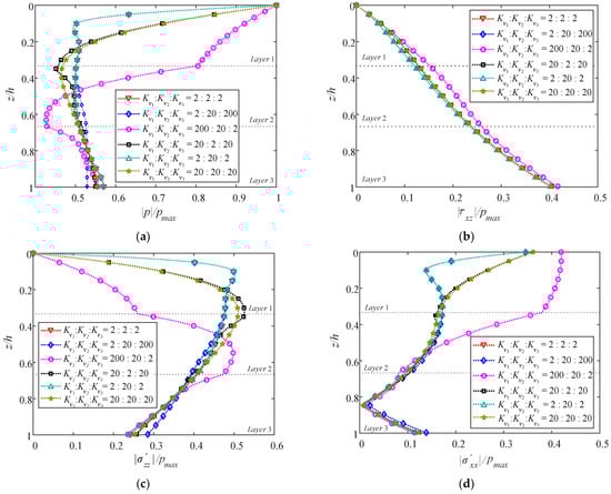
Figure 15.
Vertical distributions of normalized maximum (a) pore pressure, (b) shear stress, (c) vertical effective stress, and (d) horizontal effective stress by varying Kv1:Kv2:Kv3.
Figure 15 presents the vertical distributions of normalized maximum pore pressure of |p|, shear stress |τxz|, and vertical and horizontal effective stress || and || for the three-layered TIP seabed by varying Kv1:Kv2:Kv3. Similar to the results of the single-layered TIP seabed, Kh and Kv also significantly affect these distributions, except for |τxz|. Besides, among the six cases of Kv1: Kv2: Kv3, it is obvious that the Kh and Kv of the top layer dominate the vertical distributions of the dynamic responses. Firstly, as shown in Figure 15, these two coefficients are identical in case 1, case 2, and case 5, and their vertical distributions of the top layer and the third layer approximately coincide. Secondly, case 3, whose Kv of the top layer is as large as 2 × 10⁻² m/s, has vertical distributions distinct from the other cases.
Case 6 can be considered as an isotropic seabed. The responses of this case in interlayer differ from case 4 to some extent, though the Kh and Kv of the top and third layers are the same. The same can be said of case 1 and case 5. This is attributed to distinct Kv2. In case 4, the interlayer has a low permeability. By contrast, the permeability in case 5 is high. It can be also seen that the top and bottom layers are almost unaffected by the permeability of the interlayer. Thus, compared with Kh and Kv in the top layer, the influence caused by the permeability of the interlayer is very limited.
Figure 16 presents the maximum liquefaction depth zmax at t = 20 s by varying Kv1: Kv2: Kv3 with Kvo/Kho (o = 1,2,3), respectively, equal to 1.5, 1 and 0.8 in (a), (b), and (c). It is clear that zmax increases as Kv/Kh decreases, similar to the result of the single-layered TIP seabed. Zmax is doubled when Kvo/Kho varies from 1.5 to 1. It has been explained by Tsai [54] that highly permeable soil tends to lead to low excess pore pressure and weak liquefaction potential. According to the liquefaction criterion in Equation (45), zmax, therefore, becomes greater as Kv/Kh decreases. Moreover, cases 1, 2, and 5, where Kv and Kh of the top layer are all equal, have similar distributions of liquefaction depth and the same maximum liquefaction depths under every Kvo/Kho (o = 1,2,3). However, cases 3, 4, and 6, where the permeability coefficients of the top layer are greater, would not liquefy. Hence, this implies that the permeability coefficients of the top layer dominate zmax of the multilayered TIP seabed. Furthermore, from the enlarged details in Figure 16a–c, it can be seen that for cases 4 and 6 their zmax are the same, which is also true for cases 1 and 5. This indicates that the level of permeability in the interlayer has little effect on zmax.
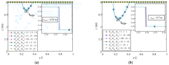
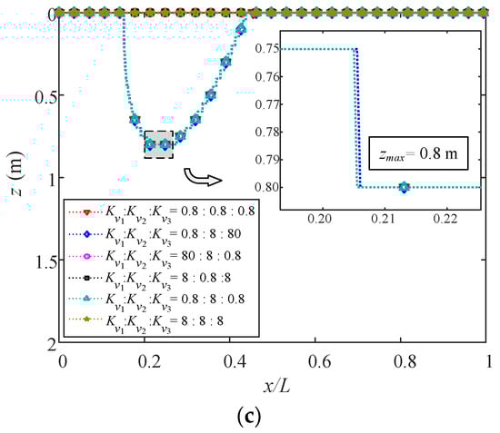
Figure 16.
Liquefaction depth along wave propagation at t = 20 s with (a) Kvo/Kho = 1.5, (b) Kvo/Kho = 1 (isotropic case), and (c) Kvo/Kho = 0.8 (o = 1,2,3).
5.2.2. Effects of Young’s Modulus
To discuss the effect of Young’s modulus on a multilayered TIP seabed, five cases are presented in Figure 17. Still, the ratio Ev/Eh of each layer is fixed to 1.5, and all Ev and Eh are relative to the typical value 2.6 × 10⁷ Pa in Table 3. Note that among the five cases, Ev1: Ev2: Ev3 = 1:1:1 corresponds to the isotropic case. Figure 17 illustrates that Young’s modulus of all three layers affects the vertical distributions of the dynamic responses in all cases. For case 2, with gradually stiffer layers, |p| declines tortuously along with the depth, while its || develops in the opposite trend. Case 3, with progressively softer layers, behaves distinctly with case 2, particularly in layers 1 and 3. It indicates that a stiffer layer tends to dissipate more pore pressure and bear more effective stress than a softer layer does.
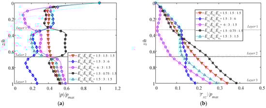
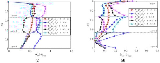
Figure 17.
Vertical distributions of normalized maximum (a) pore pressure, (b) shear stress, (c) vertical effective stress, and (d) horizontal effective stress by varying Ev1:Ev2:Ev3.
Moreover, it is interesting to observe that the developing traces of |p|, |τxz|, || and || in case 1 are in the middle of cases 4 and 5, which respectively contain a weak and a stiff intercalation.
Figure 18a–c illustrates the distributions of zmax by varying Ev1: Ev2: Ev3 with Evo/Eho (o = 1,2,3), respectively, equal to 1.5, 1, and 0.5. Similar to the results of the single-layered TIP seabed, zmax decreases as Evo/Eho (o = 1,2,3) decreases. Moreover, it can be seen that though the difference between cases 3 and 5 only lies in the top layer’s soil properties, their liquefaction depths differ remarkably. For Evo/Eho = 1.5 and Evo/Eho = 1 (o = 1,2,3), zmax of case 3, with a stiffer top layer, are 77% and 145% greater than those of case 5, respectively. For Evo/Eho = 0.5 (o = 1,2,3), case 3 is the only one that would liquefy among the five cases, as shown in Figure 18c. Hence, it once again reveals that the top layer dominates the liquefaction depth of a multilayered TIP seabed. Moreover, the stiffer the top layer, the larger the liquefaction depth. Additionally, compare cases 1, 4, and 5, their distributions of liquefaction depth are different, although their top layers are identical. However, for cases 2 and 5, which have identical properties in not only the top layer but also the middle layer, their liquefaction depths almost coincide. Therefore, it can be concluded that the middle layer also influences zmax, but the bottom layer can hardly affect the profile of zmax. The attenuating contribution of the multilayers to responses along with the depth, therefore, is demonstrated. Furthermore, comparing Figure 18a,b, zmax in the situation of Ev/Eh >1, which is common in a consolidated soil, are greater than those of Ev/Eh = 1 for all five cases. For instance, zmax of case 5 with Evo/Eho = 1.5 is 0.90 m. It is 64% greater than that with Evo/Eho = 1 which is 0.55 m. Consequently, there is a tremendous need to consider the transversely isotropic characteristics of the multilayered seabed for deeply buried subsea structures such as entrenched pipelines and undersea tunnels. Otherwise, the maximum liquefaction depth would be underestimated.
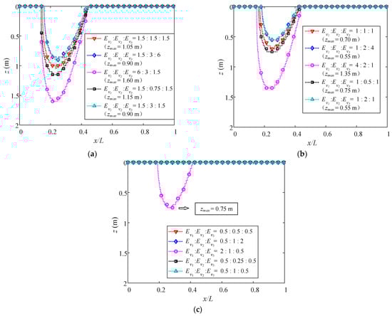
Figure 18.
Liquefaction depth along wave propagation at t = 20 s with (a) Evo/Eho = 1.5, (b) Evo/Eho = 1 (isotropic), and (c) Evo/Eho = 0.5 (o = 1, 2, 3).
5.2.3. Effects of Shear Modulus
Similar to the discussion on Young’s modulus, five cases of varying Gv1: Gv2: Gv3 are considered to investigate the effect of the shear modulus on the responses of a multilayered TIP seabed in Figure 19. The anisotropic attribute Gv/Ev of each layer equals 0.5, and all Gv and Ev are relative to the typical value 2.6 × 10⁷ Pa in Table 3. It can be noticed that the greater Gv is, the greater || and the smaller |p| will be, which is similar to the conclusion on Young’s modulus, since the shear modulus can also represent the stiffness of soil. Meanwhile, the vertical distributions of |τxz| and || are both substantially shaped by Gv.
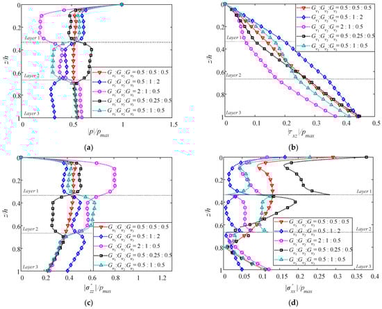
Figure 19.
Vertical distributions of normalized maximum (a) pore pressure, (b) shear stress, (c) vertical effective stress, and (d) horizontal effective stress by varying Gv1:Gv2:Gv3.
The distributions of liquefaction depth by varying Gv1: Gv2: Gv3 with Gvo/Evo (o = 1, 2, 3), respectively, equal to 0.5, 1/2.6 and 0.1, are presented in Figure 20a–c. When the ratio Gv1: Gv2: Gv3 is fixed, zmax increases as Gvo/Evo (o = 1, 2, 3) decreases. Especially for case 2, compare Figure 20b,c, zmax with Gvo/Evo = 0.1 (o = 1, 2, 3) is triple that with Gvo/Evo = 1/2.6. Therefore, it is essential to consider the transverse isotropy of soil when Gv/Ev < 2(1+v), otherwise the maximum liquefaction depth would be underestimated. With declining Gvo/Evo (o = 1, 2, 3), zmax of cases 1, 2, 4, and 5, where the top layer’s soil properties are identical, become close to each other. Hence, the influence of the Gv of multilayers decreases gradually along with the depth.
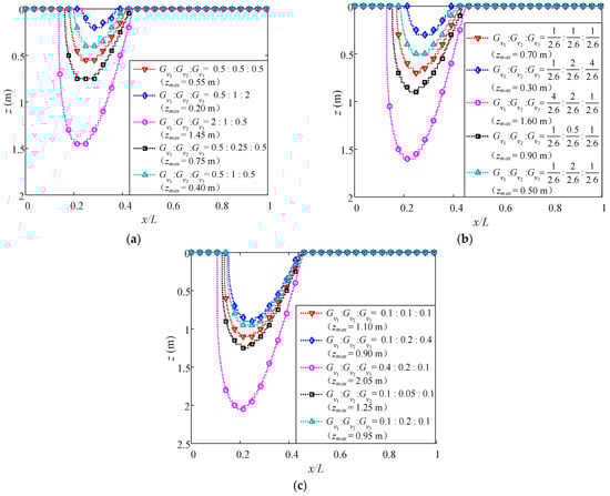
Figure 20.
Liquefaction depth along wave propagation at t = 20 s with (a) Gvo/Evo = 0.5, (b) Gvo/Evo = 1/2.6 (isotropic), and (c) Gvo/Evo = 0.1 (o = 1, 2, 3).
5.2.4. Effects of Current
The effect of U0 is presented in Figure 21 by normalizing the relative difference in soil responses between the presence and absence of a current. As stated in Section 5.1, the pore pressure and the effective stress are less sensitive to Kv/Kh than to Ev/Eh and Gv/Ev. Herein, fixed permeability coefficients of each layer Kvo = Kho = 1 × 10⁻⁴ m/s (o = 1, 2, 3) are adopted for the sake of simplicity. Three stiffer layers with Eh1: Eh2: Eh3 = 1:2:4 (where Eh1 = 2.6 × 10⁷ Pa), Evo/Eho = 1.5 and Gvo/Evo = 0.5 (o = 1, 2, 3) are assumed, while other soil parameters and wave conditions are taken from the typical values in Table 3. The subscript no-current corresponds to U0 = 0.
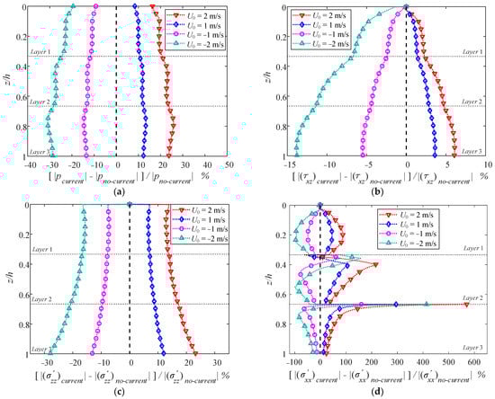
Figure 21.
Vertical distributions of the normalized relative difference in soil (a) pore pressure, (b) shear stress, (c) vertical effective stress, and (d) horizontal effective stress between the presence and absence of a current.
Figure 21 shows that U0 significantly influences the dynamic responses of the three-layered TIP seabed, especially ||, which rises up to 200% and 600% at the interface between the two adjacent layers, respectively. An opposing current in waves alleviates |p|, |τxz|, and ||, while a following current in waves aggravates those dynamic responses. For the gradually stiffer TIP multilayers treated here, the normalized relative differences grow along with the depth, which indicates that the effect of the current becomes greater towards the bedrock. Besides, when identical |U0| are examined, the waves with an opposing current (U0 < 0) will make a greater difference on the dynamic responses than that by the waves with a following current (U0 > 0), especially on |τxz|, as shown in Figure 21b.
Figure 22 and Figure 23 elucidate the distributions of zmax of the gradually stiffer layers under different U0 and wave periods T, respectively. In Figure 22, it is obvious that due to the increase in hydrodynamic pressure, a following current in waves leads to a deeper maximum liquefaction depth, while an opposing current suppresses the liquefaction. Zmax under U0 = 2 m/s and 1 m/s are 40% and 20% greater than that without a current, while zmax with U0 = −1 m/s is 40% smaller than that without a current. Hence, it can be deduced that an opposing current causes a more notable variation in the maximum liquefaction depth than a following current does, even though the current velocities are of the same magnitudes. Figure 23 tells us that as T gets shorter, zmax becomes larger.
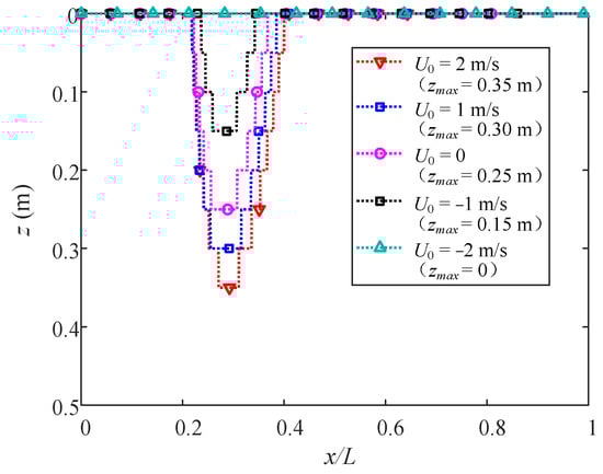
Figure 22.
Distributions of maximum liquefaction depth with different current velocities.
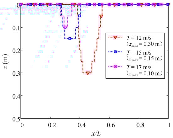
Figure 23.
Distributions of maximum liquefaction depth with different wave periods.
Figure 24 and Figure 25 show the distributions of zmax with four varying Sr and n, respectively. Zmax dramatically increases from 0 to 1.45 m as Sr decreases from 1 to 0.97, which indicates that a minor variation of merely 0.03 in Sr can lead to a distinct response to the liquefaction depth. Moreover, zmax increases as n increases, especially from 0.30 m with n = 0.3 to 1.00 m with n = 0.4. Such an increase is more than twice even though the variation of n is only 0.1. Furthermore, to investigate the effect of the rate of change induced by varying Sr in a range of 0.97, 1 and n in a range of 0.1, 0.4 on zmax, the curves of maximum liquefaction depths are illustrated in Figure 26. The four cases in Figure 24 and Figure 25 are typical scenarios on these two curves. For the vertically stiffening model, the effect of Sr becomes stronger with the increase in Sr since zmax declines faster until the liquefaction ceases. As for the porosity n, zmax increases almost linearly with n from 0.26 where the liquefaction occurs.
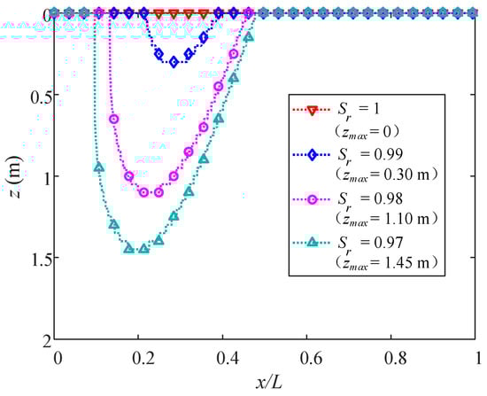
Figure 24.
Distributions of maximum liquefaction depth with different degrees of saturation.
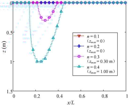
Figure 25.
Distributions of maximum liquefaction depth with different porosities.
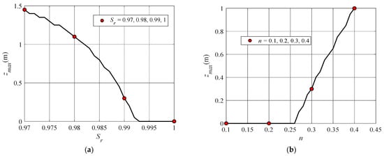
Figure 26.
Maximum liquefaction depth with varying (a) degrees of saturation and (b) porosities.
6. Conclusions
So far, the effects of the anisotropic characteristics of a multilayered TIP seabed, such as Ev/Eh, Gv/Ev and Kv/Kh, on its dynamic responses and liquefaction depth under combined wave-current loading have not been studied yet. Consequently, in this study, using the dynamic stiffness matrix method, a semi-analytical solution to the dynamic response of a multilayered TIP seabed under combined wave-current loading is developed. Verifications of the solutions to a single-layered and to a two-layered isotropic seabed are conducted analytically and experimentally. Then, a comprehensive parametric analysis of the dynamic responses and the maximum liquefaction depth of a single-layered and a multilayered TIP seabed is carried out. These parameters include the anisotropic characteristics of soil and the characteristics of waves and currents. The conclusions can be drawn as follows:
- (1)
- For both the single-layered and the multilayered TIP seabed, the dynamic responses are more sensitive to the anisotropic ratios of Ev/Eh and Gv/Ev than to Kv/Kh. The variations of Ev/Eh and Gv/Ev dramatically alter all responses of |p|, |τxz|, || and ||, but the variations of Kv/Kh have a limited influence on these responses, especially |τxz|.
- (2)
- For both the single-layered and the multilayered TIP seabed, a lower degree of quasi-saturation rate (i.e., 0.97), a higher porosity, a shorter wave period, and a following current result in a larger maximum liquefaction depth.
- (3)
- For a single-layered TIP seabed, the maximum liquefaction depths increase with decreasing Kv/Kh, Gv/Ev, and increasing Ev/Eh when Kh, Ev, and Eh are fixed, respectively, for these three ratios. Moreover, the conclusion drawn by a previous work [35] that transient liquefaction does not occur in fully saturated TIP sediments is valid, but only for an infinite thickness of the seabed, or for finite thickness with linear waves. Nonetheless, liquefaction does occur in a fully saturated and finite thickness TIP seabed under nonlinear waves.
- (4)
- For a multilayered TIP seabed, the anisotropic characteristics of the top layer dominate all dynamic responses and the maximum liquefaction depth. The contribution of stratified soil to dynamic responses and the maximum liquefaction depth gradually decays towards the bedrock. Regardless of the permeability level of the interlayer, its influence on the dynamic responses of the multilayered TIP seabed is rather limited.
- (5)
- A following current in waves aggravates the liquefaction while an opposing current suppresses the liquefaction. When a following and an opposing current are of the same magnitude, the latter results in a more notable variation on the maximum liquefaction depth than the former does. The influence of current becomes greater along with the depth, as compared to a scenario in the absence of a current.
At this stage, this study mainly considers the effects of wave–current interactions on the dynamic responses of the seabed. However, as pointed out by Zheng et al. [55], there is a certain level of probability that an earthquake might occur simultaneously with moderate or even severe sea states. It would be worthwhile, in future work, to investigate the joint earthquake-wave-current action on the seabed or structural responses, particularly involving an episode of more realistic random waves. Moreover, it should be emphasized that only in shallow and finite water depths, rather than in deep waters, does the influence of hydrodynamic pressure on soil responses deserve investigation. In this connection, future work needs to distinguish the respective influences by linear and third-order hydrodynamic pressures. To the knowledge of the authors, rare studies have considered the resonant soil responses arising from high-order Stokes waves.
Author Contributions
Methodology, X.C., X.Y.Z.; validation, X.C., Q.Z., Y.L., X.Y.Z.; investigation, X.C.; writing—original draft preparation, X.C.; writing—review and editing, X.Y.Z., X.C., Q.Z., Y.L.; funding acquisition, X.Y.Z. All authors have read and agreed to the published version of the manuscript.
Funding
The financial support received from China National Science Foundation (52071186), the Major Program of Stable Sponsorship for Higher Institutions (Shenzhen Science and Technology Commission, WDZC20200819174646001) is greatly acknowledged.
Institutional Review Board Statement
Not applicable.
Informed Consent Statement
Not applicable.
Conflicts of Interest
The authors declare no conflict of interest.
Appendix A
Appendix B
Appendix C
Appendix D
Appendix E
Appendix F
Appendix G
Equation (A34) is associated with Equation (58). Comparing it with the global stiffness matrix in Equation (56), only the last two submatrices in the last two rows of Equation (A34) differ.
References
- Christian, J.T.; Taylor, P.K.; Yen, J.K.C.; Erali, D.R. Large diameter underwater pipeline for nuclear power plant designed against soil liquefaction. In Proceedings of the Offshore Technology Conference, Houston, TX, USA, 5 May 1974; pp. 597–606. [Google Scholar]
- Damgaard, J.S.; Sumer, B.M.; Teh, T.C.; Palmer, A.C.; Foray, P.; Osorio, D. Guidelines for Pipeline On-Bottom Stability on Liquefied Noncohesive Seabeds. J. Waterw. Port Coast. Ocean Eng. 2006, 132, 300–309. [Google Scholar] [CrossRef]
- Miyamoto, T.; Yoshinaga, S.; Soga, F.; Shimizu, K.; Kawamata, R.; Sato, M. Seismic Prospecting Method Applied to the De-tection of Offshore Breakwater Units Settling in the Seabed. Coast. Eng. J. 1989, 32, 103–112. [Google Scholar] [CrossRef]
- Padgett, J.; Desroches, R.; Nielson, B.; Yashinsky, M.; Kwon, O.S.; Burdette, N.; Tavera, E. Bridge Damage and Repair Costs from Hurricane Katrina. J. Bridge Eng. 2008, 13, 6–14. [Google Scholar] [CrossRef]
- Zen, K.; Umehara, Y.; Finn, W.D.L. A case study of the wave-induced liquefaction of sand layers under damaged breakwater. In Proceedings of the 3rd Canadian Conference on Marine Geotechnical Engineering, St. John’s, NL, Canada, 11–13 June 1986; pp. 505–520. [Google Scholar]
- Lundgren, H.; Lindhardt, J.H.C.; Romhild, C.J. Stability of break waters on poros foundation. In Proceedings of the 12th In-ternational Conference on Soil Mechanics and Foundation Engineering, Rio de Janeiro, Brazil, 13–18 August 1989; pp. 451–454. [Google Scholar]
- Ulker, M.B.C.; Rahman, M.S.; Guddati, M.N. Breaking wave-induced response and instability of seabed around caisson breakwater. Int. J. Numer. Anal. Methods Geomech. 2012, 36, 362–390. [Google Scholar] [CrossRef]
- Biot, M.A. General Theory of Three-Dimensional Consolidation. J. Appl. Phys. 1941, 12, 155–164. [Google Scholar] [CrossRef]
- Biot, M.A. Theory of propagation of elastic waves in a fluid-saturated porous solid. I. Low-frequency range. Int. J. Acoust. Vibr. 1956, 28, 168–178. [Google Scholar] [CrossRef]
- Zienkiewicz, O.C.; Chang, C.T.; Bettess, P. Drained, undrained, consolidating and dynamic behaviour assumptions in soils. Géotechnique 1980, 30, 385–395. [Google Scholar] [CrossRef]
- Yamamoto, T.; Koning, H.L.; Sellmeijer, H.; Hijum, E.V. On the response of a poro-elastic bed to water waves. J. Fluid Mech. 1978, 87, 193–206. [Google Scholar] [CrossRef]
- Madsen, O.S. Wave-induced pore-pressures and effective stresses in a porous bed. Geotechnique 1978, 28, 377–393. [Google Scholar] [CrossRef]
- Seymour, B.R.; Jeng, D.S.; Hsu, J.R.C. Transient soil response in a porous seabed with variable permeability. Ocean Eng. 1996, 23, 27–46. [Google Scholar] [CrossRef]
- Yamamoto, T. Wave-induced pore pressures and effective stresses in inhomogeneous seabed foundations. Ocean Eng. 1981, 8, 1–16. [Google Scholar] [CrossRef]
- Rahman, M.S.; El-Zahaby, K.; Booker, J. A semi-analytical method for the wave-induced seabed response. Int. J. Numer. Anal. Methods Geomech. 1994, 18, 213–236. [Google Scholar] [CrossRef]
- Liu, H.; Jeng, D.S. A semi-analytical solution for random wave-induced soil response and seabed liquefaction in marine sed-iments. Ocean Eng. 2007, 34, 1211–1224. [Google Scholar] [CrossRef]
- Cheng, A.H.D.; Liu, P.L.F. Seepage force on a pipeline buried in a poroelastic seabed under wave loadings. Appl. Ocean Res. 1986, 8, 22–32. [Google Scholar] [CrossRef]
- Ulker, M.B.C.; Rahman, M.S.; Guddati, M.N. Wave-induced dynamic response and instability of seabed around caisson breakwater. Ocean Eng. 2010, 37, 1522–1545. [Google Scholar] [CrossRef]
- Ulker, M.B.C.; Rahman, M.S.; Jeng, D.S. Wave-induced response of seabed: Various formulations and their applicability. Appl. Ocean Res. 2009, 31, 12–24. [Google Scholar] [CrossRef]
- Chen, W.Y.; Jeng, D.S.; Chen, W.; Chen, G.X.; Zhao, H.Y. Seismic-induced dynamic responses in a poro-elastic seabed: Solutions of different formulations. Soil Dyn. Earthq. Eng. 2020, 131, 106021. [Google Scholar] [CrossRef]
- Jeng, D.S.; Rahman, M.S.; Lee, T.L. Effects of Inertia Forces on Wave-Induced Seabed Response. In Proceedings of the 19th International Offshore and Polar Engineering Conference, Brest, France, 30 May–4 June 1999. [Google Scholar]
- Jeng, D.S.; Rahman, M.S. Effective stresses in a porous seabed of finite thickness: Inertia effects. Can. Geotech. J. 2000, 37, 1383–1392. [Google Scholar] [CrossRef]
- Jeng, D.S.; Lee, T.L. Dynamic response of porous seabed to ocean waves. Comput. Geotech. 2001, 28, 99–128. [Google Scholar] [CrossRef]
- Gatmiri, B. Simplified finite element analysis of wave-induced effective stresses and pore pressures in permeable sea beds. Geotechnique 1990, 40, 15–30. [Google Scholar] [CrossRef]
- Thomas, S.D. A finite element model for the analysis of wave induced stresses, displacements and pore pressures in an un-saturated seabed II: Model verification. Comput. Geotech. 1995, 17, 107–132. [Google Scholar] [CrossRef]
- Schumacher, T.; Higgins, C.; Bradner, C.; Cox, D.; Yim, S.C. Large-scale Wave Flume Experiments on Highway Bridge Su-perstructures Exposed to Hurricane Wave Forces. In Proceedings of the 6th National Seismic Conference on Bridges and Highways, Charleston, WV, USA, 27–30 July 2008. [Google Scholar]
- Onorato, M.; Osborne, A.R.; Serio, M.; Cavaleri, L.; Brandini, C.; Stansberg, C.T. Extreme waves, modulational instability and second order theory: Wave flume experiments on irregular waves. Eur. J. Mech. 2006, 25, 586–601. [Google Scholar] [CrossRef]
- Kirca, V.S.O.; Sumer, B.M.; Fredsoe, J. Influence of Clay Content on Wave-Induced Liquefaction. J. Waterw. Port Coast. Ocean Eng. 2014, 140, 04014024. [Google Scholar] [CrossRef]
- Tzang, S.Y. Unfluidized soil responses of a silty seabed to monochromatic waves. Coast. Eng. 1998, 35, 283–301. [Google Scholar] [CrossRef]
- Ye, J.H.; Jeng, D.S. Response of Porous Seabed to Nature Loadings: Waves and Currents. J. Eng. Mech. 2012, 138, 601–613. [Google Scholar] [CrossRef]
- Zhang, Y.; Jeng, D.S.; Gao, F.P.; Zhang, J.S. An analytical solution for response of a porous seabed to combined wave and current loading. Ocean Eng. 2013, 57, 240–247. [Google Scholar] [CrossRef]
- Liu, B.; Jeng, D.S.; Zhang, J.S. Dynamic Response in a Porous Seabed of Finite Depth to Combined Wave and Current Loadings. J. Coast. Res. 2014, 30, 765–776. [Google Scholar]
- Cheng, H.D. Material coefficients of anisotropic poroelasticity. Int. J. Rock Mech. 1997, 34, 199–205. [Google Scholar] [CrossRef]
- Jeng, D.S. Effect of cross-anisotropic behaviour on wave-induced seabed response. Géotechnique 1998, 48, 555–561. [Google Scholar] [CrossRef]
- Jeng, D.S. Soil Response in Cross-Anisotropic Seabed due to Standing Waves. J. Rock Mech. Geotech. 1997, 123, 9–19. [Google Scholar] [CrossRef]
- Zhang, Z.; Pan, E. Time-harmonic response of transversely isotropic and layered poroelastic half-spaces under general buried loads. Appl. Math. Model. 2020, 80, 426–453. [Google Scholar] [CrossRef]
- Ye, Z.; Ai, Z.Y. Dynamic analysis of multilayered unsaturated poroelastic media subjected to a vertical time-harmonic load. Appl. Math. Model. 2021, 90, 394–412. [Google Scholar] [CrossRef]
- Li, X.; Zhang, Z.; Pan, E. Wave-induced dynamic response in a transversely isotropic and multilayered poroelastic seabed. Soil Dyn. Earthq. Eng. 2020, 139, 106365. [Google Scholar] [CrossRef]
- Sparks, A.D.W. Theoretical considerations of stress equations for partly saturated soils. In Proceedings of the 3rd Regular Conference for Africa on Soil Mechanics and Foundation Engineering, Salisbury, UK, 2–9 June 1963; pp. 215–218. [Google Scholar]
- Laing, B. Consolidation of Compacted and Unsaturated Clays. Géotechnique 1965, 15, 267–286. [Google Scholar]
- Chang, C.S.; Duncan, J.M. Consolidation analysis for partly saturated clay by using an elastic-plastic effective stress-strain model. Int. J. Numer. Anal. Methods Geomech. 1983, 7, 39–55. [Google Scholar] [CrossRef]
- Biot, M.A. Mechanics of Deformation and Acoustic Propagation in Porous Media. J. Appl. Phys. 1962, 33, 1482–1498. [Google Scholar] [CrossRef]
- Verruijt, A. Elastic Storage of Aquifers. In Flow through Porous Media; Wiest, R.J.M.D., Ed.; Academic Press: New York, NY, USA, 1969; pp. 331–376. [Google Scholar]
- Esrig, M.I.; Kirby, R.C. Implications of gas content for predicting the stability of submarine slopes. Mar. Geotechnol. 1977, 2, 81–100. [Google Scholar] [CrossRef]
- Hsu, H.C.; Chen, Y.Y.; Hsu, J.R.C.; Tseng, W.J. Nonlinear water waves on uniform current in Lagrangian coordinates. J. Nonlinear Math. Phys. 2009, 16, 47–61. [Google Scholar] [CrossRef]
- Liu, H.; Pan, E. Time-harmonic loading over transversely isotropic and layered elastic half-spaces with imperfect interfaces. Soil Dyn. Earthq. Eng. 2018, 107, 35–47. [Google Scholar] [CrossRef]
- Feng, S.; Ding, X.; Zheng, Q.; Chen, Z. Extended stiffness matrix method for horizontal vibration of a rigid disk embedded in stratified soils. Appl. Math. Model. 2020, 77, 663–689. [Google Scholar] [CrossRef]
- Qi, W.G.; Li, C.F.; Jeng, D.S.; Gao, F.-P.; Liang, Z.D. Combined wave-current induced excess pore-pressure in a sandy seabed: Flume observations and comparisons with theoretical models. Coast. Eng. 2019, 147, 89–98. [Google Scholar] [CrossRef]
- Olabarrieta, M.; Medina, R.; Castanedo, S. Effects of wave-current interaction on the current profile. Coast. Eng. 2010, 57, 643–655. [Google Scholar] [CrossRef]
- Le Méhauté, B. An Introduction to Hydrodynamics and Water Waves; Springer: Berlin/Heidelberg, Germany, 1976; p. 205. ISBN 978-3-642-85569-6. [Google Scholar]
- Zen, K.; Yamazaki, H. Mechanism of wave-induced liquefaction and densification in seabed. Soils Found. 1990, 30, 90–104. [Google Scholar] [CrossRef]
- Rahman, M.S. Wave-induced instability of seabed: Mechanism and conditions. Mar. Geotechnol. 1991, 10, 277–299. [Google Scholar] [CrossRef]
- Terzaghi, K.; Peck, R.B.; Mesri, G. Soil Mechanics in Engineering Practice, 3rd ed.; John Wiley & Sons, Inc.: New York, NY, USA, 1996; ISBN 978-0-471-08658-1. [Google Scholar]
- Tsai, C.P. Wave-induced liquefaction potential in a porous seabed in front of a breakwater. Ocean Eng. 1995, 22, 1–18. [Google Scholar] [CrossRef]
- Zheng, X.Y.; Li, H.B.; Rong, W.D.; Li, W. Joint earthquake and wave action on the monopile wind turbine foundation: An experimental study. Mar. Struct. 2015, 44, 125–141. [Google Scholar] [CrossRef]
Publisher’s Note: MDPI stays neutral with regard to jurisdictional claims in published maps and institutional affiliations. |
© 2022 by the authors. Licensee MDPI, Basel, Switzerland. This article is an open access article distributed under the terms and conditions of the Creative Commons Attribution (CC BY) license (https://creativecommons.org/licenses/by/4.0/).