Numerical Analysis of Single-Particle Motion Using CFD-DEM in Varying-Curvature Elbows

Abstract

Centrifugal pumps are the critical components in deep-sea mining. In order to investigate the particle motion in the curved channel of the impeller, three different types of curvature conform to blade profile to simplify the impeller design of pumps. A numerical study is conducted to investigate the flow field in a varying-curvature channel for solid-liquid two-phase flow. The flow of particles within the varying curvature channel is studied by combining the discrete element method (DEM) with computational fluid dynamics (CFD) and a comparison with Particle Image Velocimetry (PIV) test results. The results show that a polyhedral mesh with a small mesh number yields very accurate results, which makes it very suitable for CFD-DEM. Based on this method, the movement of a single particle is compared and analyzed, and the particle-motion law is obtained. The effects of the curvature ratio Cr and area ratio Ar on the motion law for a single particle are studied, and the simulation results are analyzed statistically. The results show that the effect of Cr on both the particle slip velocity and the turbulent kinetic energy only changes its strength, while the distribution law does not change significantly. Compared with the curvature ratio Cr, the area ratio Ar has a greater impact on the particles, and its distribution law becomes clearly different. As the area ratio Ar increases, the arc radius and length of the corresponding particle trajectory decrease.

1. Introduction

The deep sea is abundant in mineral resources that are scarce on land, and the exploration of marine mineral resources continues to show promising development prospects [1,2,3]. When harvesting marine mineral resources, the transport/flow of particles via pumps is typically involved [4]. The centrifugal pump is practically irreplaceable in the required conveying system. However, the wear of centrifugal pumps is a major cause of pump failure. More specifically, the wear of flow-passage components in two-phase flow pumps refers to the loss of surface material on the wall of flow-passage components due to the impact of solid particles in the liquid. The degree of wear is closely related to the particle trajectory, particle velocity distribution, and the flow field in the pump. Moreover, the wear of particles can change the performance of the pump, increase flow loss, and aggravate wear, which can affect both the service life and reliability of the pump. Therefore, studying particle wear is important to improve the flow field in two-phase flow pumps.

Many studies of two-phase flow have already been published. Traditional solid-liquid two-phase flow methods (e.g., the two-fluid model of the Euler-Euler method) assume that the solid phase is a continuous pseudo fluid, and local averages are used. Therefore, there are some limitations to the prediction of the non-uniform characteristics of solids. Recently, the CFD-DEM method has been widely applied to study the coupled flow between the solid and continuous phase. The discrete element method (DEM), which was proposed by Cundall [5,6,7], is a display solution method that directly solves discrete particles without the above assumptions. This makes it possible to obtain rich micro particle information—even particle information that is difficult to measure in a test. It tracks the force and motion trajectories of each discrete particle in the system in Lagrange coordinates. The interaction forces between particles (and between particles and wall) are determined by the simplified contact-mechanics model. Therefore, the DEM has the important advantage that it allows the calculation of the flow of particles with a high accuracy as well as the collision behavior of particles. At present, it is mainly used for particle transportation, rock drilling, bucket digging, particle reactions, pipeline wear, etc. [8,9,10].

Due to the advantages of the DEM method with respect to solid particle calculation, many researchers use this method for coupling with a continuous phase [11,12,13]. Zhao [14] simulated the gas-solid flow in a two-dimensional downer using the CFD-DEM method. Their results showed good agreement with the experimental findings. Afkhami et al. [15] used the coupled LES-DEM to study turbulent particle-laden flows in a channel. The group results showed that the particle agglomeration is enhanced both in the near-wall region and in the buffer region within the channel. Chen et al. [16] simulated horizontal pipelines using the CFD-DEM coupling method by conveying different shapes of particles and different concentrations. This was done to obtain the relationship between the effect of the particle characteristics on the flow characteristics. Li et al. [17] investigated the particle-backflow blockage problem using the CFD-DEM for a single-stage centrifugal pump. The group showed the effect of particle size on a blockage in the pump. Furthermore, Hu et al. [18] applied the coupled CFD-DEM simulations to clarify the solid-liquid two-phase flow in two-stage centrifugal pumps for different particle sizes with constant particle concentrations. Deng et al. [19] investigated the hydrodynamic (and coarse) kinetic behavior of the particles in the pump for slurry transfer using the coupled CFD-DEM simulation. The group determined the slurry transport characteristic curves as well as the particle transport and distribution characteristics of six-stage centrifugal pumps. Nonetheless, applications of the CFD-DEM for solid-liquid two-phase pumps are still few or none. The main reason for this is that the calculation process, which is associated with the DEM for liquid-solid coupling, is relatively slow. To solve this problem, a polyhedron grid is used in this paper, which significantly shortened the calculation time.

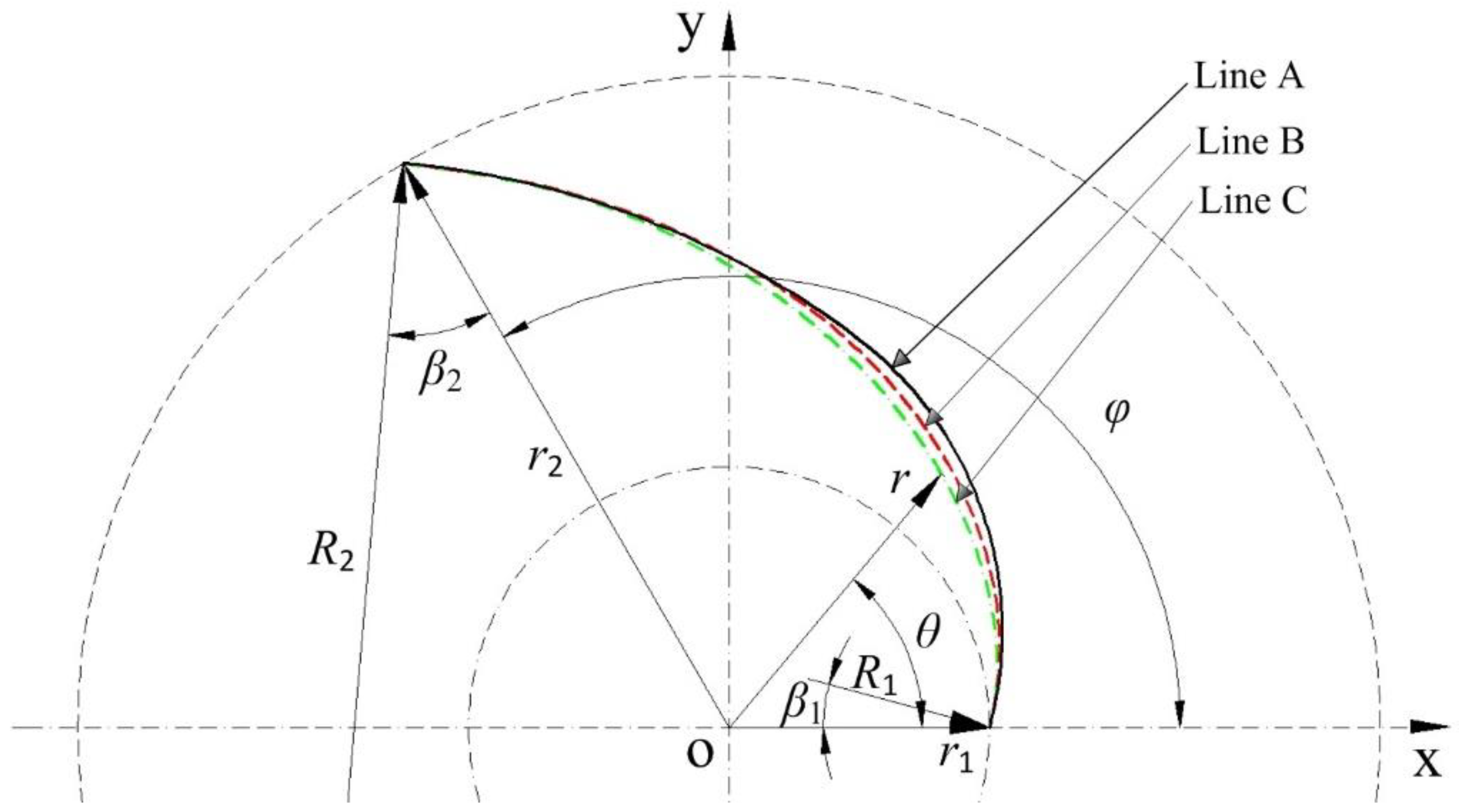
In fluid machinery, curved channels are commonly used—particularly in pumps [20,21]. However, the curvature changes of the channel in the rotating impeller are more complex, and the channel is also affected by the rotation factors. This makes it difficult to accurately predict the flow of the impeller. Compared with the curved channels in hydraulic systems, a simple pipe flow is basically only affected by a single factor. For example, the rotation of the straight pipe is only affected by the rotation speed, and the static curved channel is only affected by the curvature of a single arc. Therefore, the flow channels in fluid machinery can be simplified to curvature flow channels. Many researchers have compared the simplified flow passage with the impeller’s flow passage [22,23]. Macfarlane et al. [24] conducted an experimental study of rotating rectangular tubes with different area ratios to find the relationship between secondary flow and the turbulent boundary layer with a zero-pressure gradient. This provides a reference for the design of a centrifugal impeller. Tsujita et al. [25] numerically studied the flow in curved pipes (square cross-section) and applied the loss mechanism to the impeller channel. Guleren et al. [26] used the LES method to compare and study the flow in the transition zone (from turbulence to laminar flow) of the inner axial flow-channel of a straight pipe, a U-pipe, and a typical centrifugal compressor impeller. In addition, the group investigated the effect of both channel curvature and rotation. Casey et al. [27] proposed a new through-flow method based on the streamline curvature, which was successfully used for the meridional flow-channel (axial plane) of mixed flow pumps and turbines. With this method, both the leading and trailing edges of the blade were rectangular pipes in the study. This has important benefits for the preliminary design of multistage axial flow machinery.

In previous studies [28,29], the overall flow development in ducts was studied in depth. This manuscript aims to extend the above design ideas and methods to solid-liquid two-phase flow. The curved channel is used to study the varying curvature profile of the impeller, with the aim of providing a reference for the design of the impeller. In this study, the basic idea of the discrete element method is introduced first. Then, the effect of the polyhedron grid on solid-liquid two-phase coupling is verified, and the CFD-DEM simulation is performed. This is in good agreement with the experimental results. Then, the single-particle motion in the varying curvature elbow is compared and analyzed, and the particle motion law is determined. The effect of the curvature ratio Cr and the area ratio Ar on the single-particle motion law are studied. Furthermore, a statistical analysis of the simulation results is carried out.

The paper is organized as follows: the problem description and experiment set-up are clarified in Section 2. Section 3 describes the numerical simulation and validation. The effects of the curvature ratio Cr and the aspect ratio Ar are analyzed in Section 4. Conclusions are summarized in Section 5.

2. Model Description and Experiment Set-Up

2.1. Problem Description

The computational geometric model, which is used in this paper, is shown in Figure 1. It includes the bending section, the inlet extension, and the outlet extension. Because the width and the height of the pipe flow section remain unchanged, the polar angle associated with each flow section in the bending section is defined as the polar angle θ of the curvature line of its inner wall. The curvature ratio and aspect ratio are defined as:

$$Cr=\frac{D_h}{R_c}=\frac{D_h}{R_{ICW}+b/2}$$

(1)

$$Ar=\frac{a}{b}$$

(2)

where, a is the height of the pipe and b denotes the width of the pipe. R_c is the average radius of curvature, and D_h is the hydraulic diameter of the varying curvature duct.

$$D_h=\frac{2ab}{a+b}=\frac{2a}{Ar+1}$$

(3)

A comparison of three varying curvature profiles is shown in Figure 2. The three types of curves are denoted as circular line (A-CL), spiral line (B-SL), and involute line (C-IL). More details for these models are given in Li et al. [28,29].

In this paper, the calculation scheme is based on these definition relations. This makes it possible to compare the effects of both the curvature ratio Cr and area ratio Ar on the flow in the pipe. A total of nine cases were considered to study the effect of Cr and Ar, see

Table 1. Summary of cases studied [29].

Case	a/mm	Dh/mm	RICW	Ar
1	35	48.7	A-CL	0.4
2	35	35	A-CL	1
3	80	48.7	A-CL	2.3
4	35	48.7	B-SL	0.4
5	35	35	B-SL	1
6	80	48.7	B-SL	2.3
7	35	48.7	C-IL	0.4
8	35	35	C-IL	1
9	80	48.7	C-IL	2.3

.

2.2. Experiment Set-Up

The schematic diagram of the PIV set-up of varying curvature elbows is shown in Figure 3. The facility mainly included a pipe flow system and a PIV test system. The upstream and downstream of the curved duct were PVC circular pipes with a diameter of 75 mm, while a rectangular cross-section (35 mm (a) × 80 mm (b)) was adopted for varying curvature elbow sections, which were made of plexiglass. A transition section converted flow from the rectangular section of the plexiglass pipe into the circular section of the PVC so that the flow could transition smoothly between different sections. Two lengths of 1.5 m ≈ 31D_h long straight ducts were used before and after the varying curvature elbow to ensure the full development of the inlet and outlet flow conditions. A submersible pump was placed in the tank to drive the whole pipeline circulation system. Two values were respectively installed at the inlet and outlet of the loop to control the flow rate. The flow collection was completed by an electromagnetic flowmeter.

A two-dimension Lavision PIV system was adopted to test the plane of the middle section of the varying curvature elbow (z = 0). The neutral spherical ^®110P8 (LaVision Inc, Göttingen, Germany) hollow glass sphere was used as a tracer particle with an average diameter of 15 μm. The particle image was recorded by a 12-bit CCD camera with a resolution of 1600 × 1200 pixels, and the highest frequency was 15 Hz. A 530 nm band-pass filter was installed in front of the CCD camera lens so that the CCD camera could only accept 532 nm laser light with an error within 1 nm wavelength, which reduced the image background noise. The target flow field was divided into two overlapping sections: L₁ (θ = 10°~80°) and L₂ (θ = 70°~120°). Both sections were 260 mm × 195 mm; therefore, the flow field of the whole elbow could be obtained. A set of 1680 pairs of particle images were adopted for each case to obtain the ensemble-averaged velocities.

3. Numerical Simulation and Validation

3.1. Numerical Methodology

According to Newton’s second law, the motion of particles can be divided into two different types in a given system: translation and rotation. Particles may collide with adjacent particles or the wall at any time in the process of these two types of motion, and the particles interact with their surrounding fluid to exchange momentum and energy. Therefore, the solution for the solid-liquid two-phase CFD-DEM is divided into three parts: solution of the continuous phase, solution of the discrete phase, and two-phase coupling.

The continuous phase mainly represents a solution of the Navier Stokes equation, and its mass and momentum conservation equations are:

$$\frac{\partial \rho }{\partial t}+\nabla ·(\rho u)=0$$

(4)

$$\frac{\partial (\rho u)}{\partial t}+\nabla ·(\rho uu)=-\nabla p+\nabla ·(\mu \nabla u)+\rho g-F_{pf}$$

(5)

where, F_pf represents the momentum exchange between the continuous phase and discrete phase. It is a pair of interaction forces, with F_fp in the motion equation for the discrete phase, which is associated with coupling between two phases.

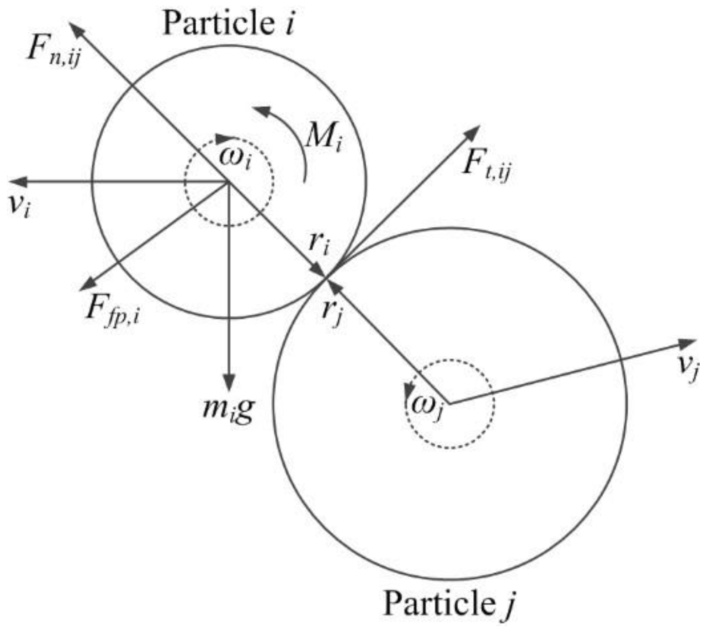
The discrete phase mainly solves the force in the particle collision process via the contact model. The particle acceleration can be calculated by using Newton’s second law and then updating both the particle velocity and displacement. According to the force analysis of particle i (see Figure 4), the corresponding momentum conservation and angular momentum conservation equations are:

$$m_i\frac{d{v}_i}{dt}={\displaystyle \sum _j(F_{n,ij}+F_{t,ij})+m_{i}g+F_{fp,i}}$$

(6)

$$\frac{d}{dt}{I}_i{\omega }_i={\displaystyle \sum _j(r_i\times F_{t,ij}+M_i)}$$

(7)

where, m_i and v_i are the mass (kg) and velocity (m/s) of particle i, respectively; g is the gravity acceleration (m/s²); F_n,ij is the normal contact force (N) between particle i and element j; F_t,ij is its tangential contact force (N). I_i and ω_i are the moment of inertia (kg·m²) and angular velocity (rad/s) of particle i, respectively. r_i is the radius of particle i (m). F_fp denotes the force from a liquid relative to particle i (N). M_i represents the rolling friction torque (N·M).

From the above continuous and discrete phase-governing equations, it is found that interphase interaction occurs between solid and liquid phases, which can exchange mass, momentum, and energy. According to Newton’s third law, the liquid exerts a force on the particles, while the particles can act on the fluid. Therefore, the two-way coupling method was used to describe the interaction between the two phases. In general, the effect of interphase action on the continuous phase can be ignored for dilute-phase particles. Therefore, the Schiller-Naumann drag model is used for the one-way coupling solution in this paper. The force, which is exerted by the fluid on particles, only considers the drag force and pressure gradient force, but ignores the force exerted by other fluids.

3.2. Verification of Grid Scheme

The generation scheme and its independence analysis are shown in

Table 2. Polyhedral mesh independent analysis.

Polyhedron Mesh	Mesh_1	Mesh_2	Mesh_3	Mesh_4	Mesh_5
Number of Elements	36,695	81,650	157,984	550,842	762,336
Number of Faces	154,171	358,656	741,966	2,848,322	4,025,597
Number of Vertices	94,193	228,087	497,765	2,049,592	2,935,943
Friction Coefficient f	0.016116	0.016963	0.017477	0.018092	0.018838

. With the same simulation settings, the grid schemes in Table 2 were calculated. The friction coefficients of the import and export were obtained, in which the friction coefficient f is calculated by the Darcy–Weisbach formula:

$$f=\frac{\Delta p}{\frac{1}{2}\rho u_b^2}\frac{D_h}{L}$$

(8)

where Δp is the pressure drop of the inlet and outlet (Pa), D_h is the hydraulic diameter of the pipeline (m), L is the length of the centerline of the flow channel (m), ρ is density (kg/m³), and u_b is the average velocity (m/s).

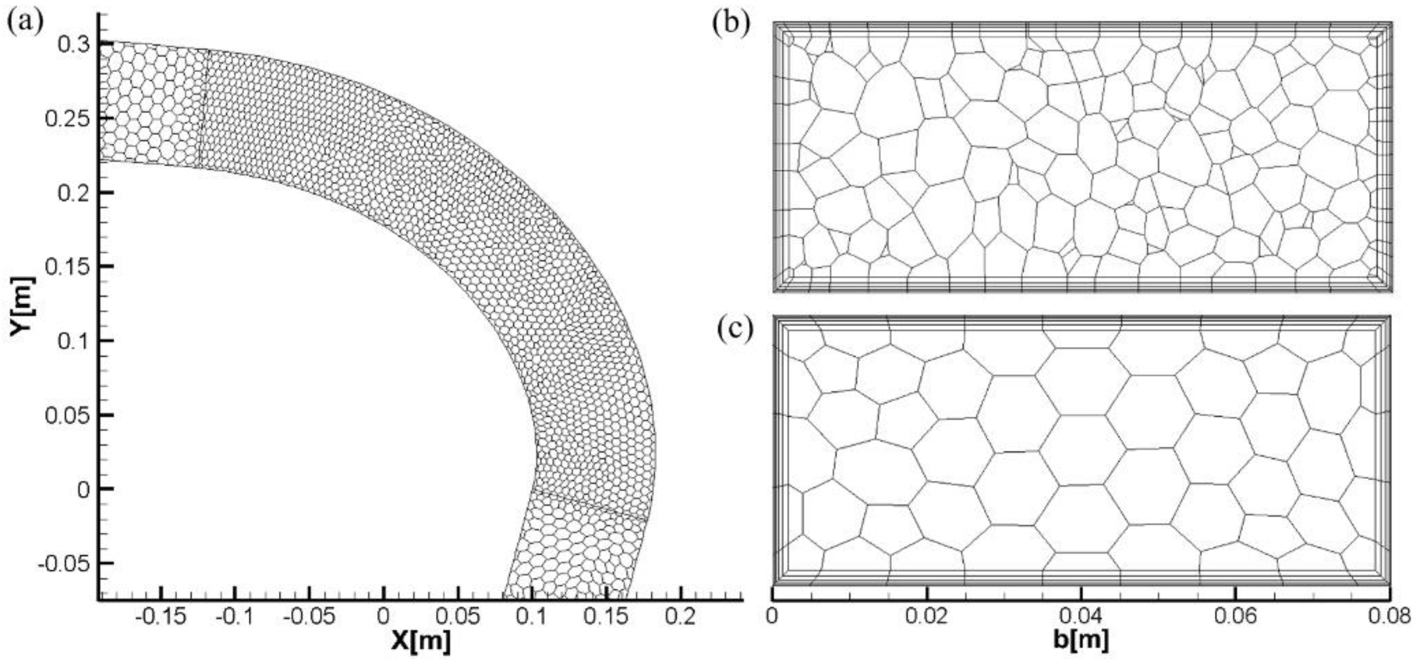
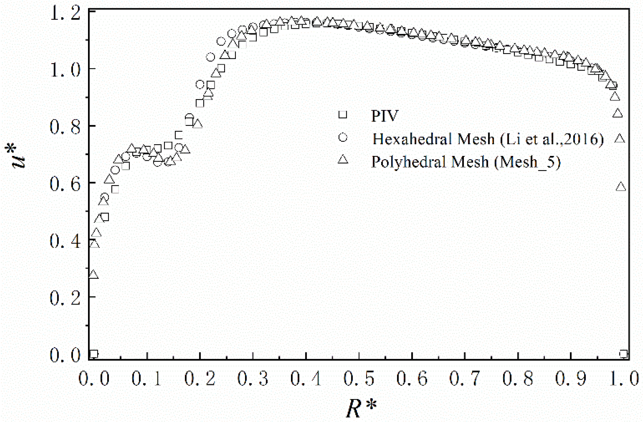
Taking the C-IL tube as an example, at Re_b = 1.4 × 10⁵, the optimal number of hexahedral meshes is 3–3.5 million cells [29]. Compared to the same varying curvature pipeline, the number of polyhedral meshes is lower. Therefore, the polyhedron grid appears more suitable for the CFD-DEM. To better understand the benefits of the polyhedral grid, the velocity fields, which were calculated by polyhedral grids and hexahedral grids, are compared with those obtained using PIV. Taking θ = 80° as an example, the comparison results are shown in Figure 5.

The dimensionless radius R* = (R_i – R_ICW)/b. At R* = 0.1~0.25, the dimensionless axial velocity u*, which was calculated using polyhedrons, reached the accuracy for hexahedrons, which is close to the PIV result. Due to the large effect error of the velocity gradient, this reflects the more accurate characteristics for polyhedrons in the calculation gradient and the local flow conditions. At R* = 0.2~0.3, it represents the intersection of the curvature vortex and the basic vortex. Furthermore, the secondary flow-velocity flows back from the inner curvature wall (ICW) to the outer curvature wall (OCW) when the axial velocity increases from the trough to the maximum. In addition, the calculation accuracy with polyhedrons is even higher than for the hexahedron grid.

Even though there are fewer cells in the polyhedron grids, the scheme of Mesh_5 still requires more computing power and time with the CFD-DEM simulation. Therefore, further dilution was carried out based on the grid volume. The simulation accuracy error of Mesh_2 in

Table 3. Boundary layer mesh refinement.

Thickness × 10−4 m	1.1	1.5	1.8	2.2	3	3.8
Friction Coefficient f	0.016215	0.017157	0.017223	0.017419	0.01775	0.01801
y+	1.6~14	0.4~10.6	7~21.1	9~25	12.3~32.1	11.1~38.7

is 9.1%, but the number of grids is nearly 1/9 of Mesh_5. To fully account for computing accuracy and computing resources, the grid of Mesh_2 was further refined. In the mesh refinement scheme, the effect of boundary layers was taken into account, see Table 3.

A mixed treatment (all y+ wall treatment) was used to deal with the wall boundary, and the appropriate wall function was automatically selected based on the value of y+. As shown in Table 3, with increasing thickness of the first layer of the boundary layer, the friction coefficient f also increased. However, the deviation between the axial velocity and PIV became larger, see Figure 6. At R* = 0.1~0.5, the larger the y+ value, the larger the error at the predicted flow separation and gradient. Therefore, by carefully weighing the friction coefficient and velocity field prediction results, the polyhedral grid of Mesh_ 2 was selected. The thickness of the first layer of the boundary layer was 1.5 × 10⁻⁴ m, and its y+ value was in the range 0.4~10.6. In addition, the curvature elbow section was refined. The final volume grid is shown in Figure 7, and the relative error of the accuracy of the friction coefficient f was 8%. The solution-finding time was reduced by nearly 1/10, and its simulation accuracy was within an acceptable range.

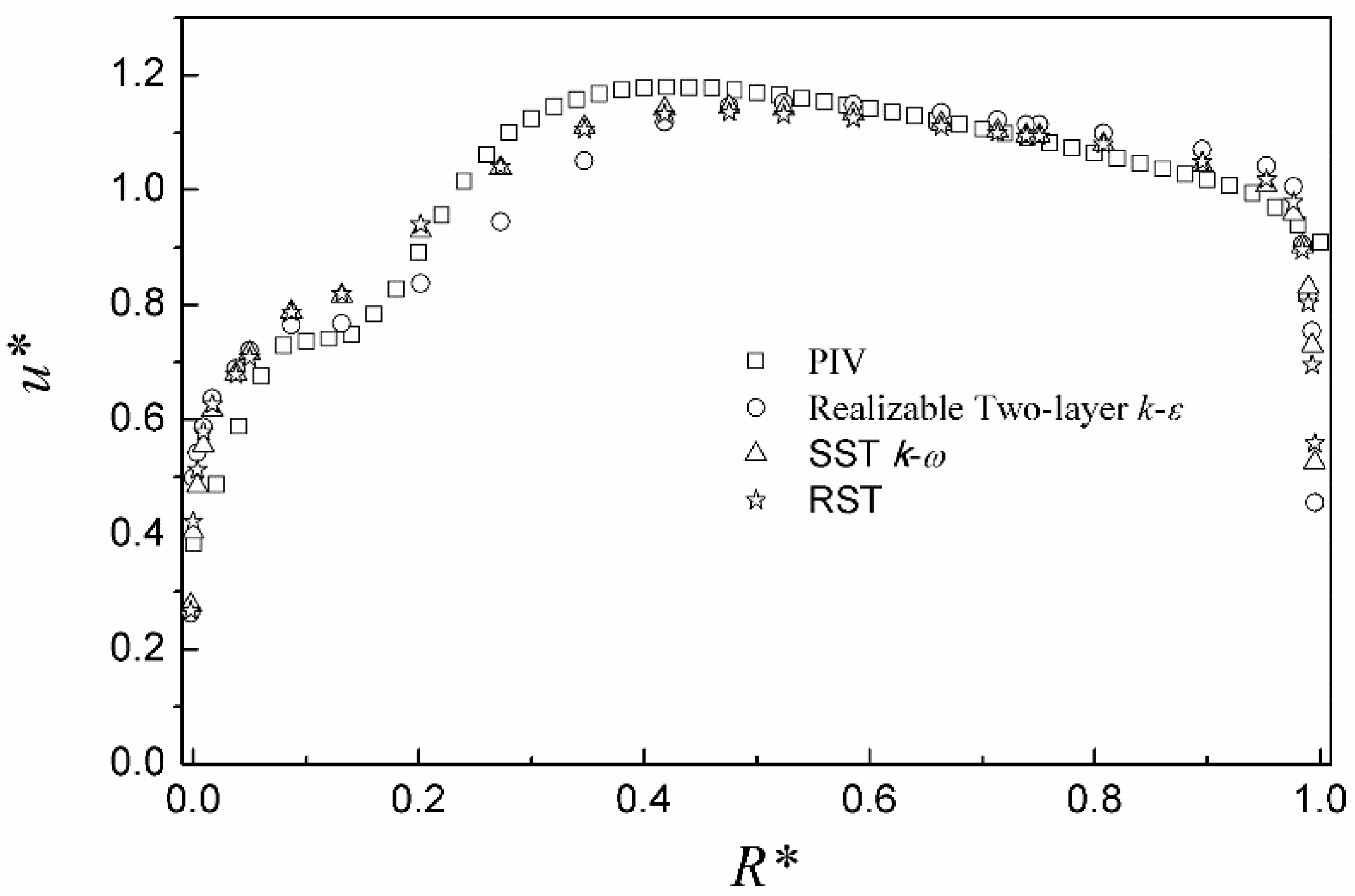
3.3. Validation of Turbulence Model

Using the C-IL tube as the test object, the realizable two-layer k-ε model, SST k-ω model, and Reynolds stress model (RST) were selected for coupling with DEM. At Re_b = 1.4 × 10⁵, the friction coefficient f was obtained by using the above three turbulence models, as shown in

Table 4. Comparison of friction coefficient obtained by the different turbulent models.

Turbulence Model	Realizable Two-Layer k-ε	SST k-ω	RST
Friction Coefficient f	0.016223	0.017157	0.016495
Relative Error	13%	8%	12%

. The relative error of the friction coefficient predicted by the SST k-ω model was the smallest, less than 10%, while the relative error of the realizable two-layer k-ε model was the largest, followed by the RST model.

Figure 8 shows the axial velocity of three turbulence models at θ = 80° compared with PIV results. As shown in Figure 8, there are differences between the predicted u* of the three models and the PIV results at the positions of the ICW curvature vortex and basic vortex (R* = 0.1~0.4). The error of maximum axial velocity u_a,max predicted by the realizable two-layer k-ε model was the largest, while the other two models were very close.

3.4. Numerical Set-Up

In this study, the continuous phase for a single particle was solved using the Euler method, and the discrete phase was solved with the Lagrange method. Moreover, the Hertz-Mindlin non-sliding contact model was adopted for the discrete phase collision. STAR-CCM+ was used for the polyhedron mesh generation, and unsteady calculation was used for the simulation in this paper. The SST k-ω model was selected as the turbulence model. The boundary conditions were uniform flow velocity at the inlet of the curved duct, applied no-slip boundary conditions on the duct walls, and a pressure outlet condition of the curved duct. The unsteady calculation for clean water was performed in 0 ~ 1 s, and the release of single particles started at 1 s. The time for particles to leave the pipeline was at least 1 s. Therefore, the simulation time was set to 3 s. In this way, particles can complete the simulation calculation of the complete flow in the pipeline. The single particle was set to spherical, and its diameter was d_p = 1 mm. The physical and mechanical properties of the particles are shown in

Table 5. Particle parameters.

Parameter	Symbol	Unit	Value
Density	ρp	kg/m3	1000
Diameter	dp	mm	1
Poisson Ratio	vi	(-)	0.28
Young’s Modulus	Ei	MPa	10
Static Friction Coefficient	Cfs	(-)	0.15
Normal Recovery Coefficient	Nn	(-)	0.5
Tangential Recovery Coefficient	Nt	(-)	0.5
Rolling Friction Coefficient	μr	(-)	0.01

. The release position was the middle of the ducts. The fluid density was ρ_p = 1000 kg/m³ and the Reynolds number was Re_b = 1.4 × 10⁵.

4. Results and Discussion

4.1. Effect of the Curvature Ratio

The curvature ratio Cr of the A-CL tube, B-SL tube, and C-IL tube were compared. The area ratio was Ar = 0.4, and the CFD-DEM coupling trajectory is shown in Figure 9. It can be seen from the figure that the trajectory of the particles corresponds to the change law of the ICW curve. The curvature radian for C-IL was the smallest, followed by B-SL, and A-CL was the largest. Due to the existence of curvature, the particles are not only affected by the fluid drag force and pressure gradient force, but also affected by the curvature centrifugal force generated by the curvature geometry. Affected by the centrifugal force, the particles are obviously biased towards OCW at the outlet of the curvature duct, so the particles are more likely to collide with the outer wall of the curvature duct.

Due to the effect of curvature, the length of the particle trajectory in the three ducts is different, and the time spent flowing through the ducts is also different.

Table 6. Effects of Cr on particle motion time through the whole duct.

	Release Time t1(s)	Curvature Inlet tin(s)	Curvature Outlet tout(s)	Outlet t2(s)
A-CL	1.000000	1.205250	1.341487	1.620885
B-SL	1.000000	1.205573	1.340182	1.618068
C-IL	1.000000	1.204720	1.339754	1.624056

shows the time spent for the three curvatures and particles flowing through the ducts with different curvatures. The C-IL tube is the first to reach the curvature inlet, and the C-IL tube is the first to leave the curvature outlet. However, the time consumption for B-SL in the varying curvature sections was the shortest, which indicates that the curvature ratio also affects the velocity of the particles.

The most important components of the particle velocity are the slip velocity and the settling velocity. The former determines the particle’s Reynolds number and affects forces such as the drag force, while the latter affects the accumulation and hydraulic transport capacity of the particles. The effect of the curvature ratio Cr on the slip velocity of the particles is shown in Figure 10. Taking the simulation time as a reference, the variation trends of the slip velocity in different variable-curvature tubes are the same. After the particles were released at 1 s, there was a trough (about 1.1 s) in the straight pipe section. When they entered the variable curvature elbow (t ≈ 1.2 s), there were two troughs and one peak (see the local enlarged view of Figure 10). Then, there was a peak near the outlet curvature of the varying curvature elbow (1.3 s < t < 1.35 s) and a trough in the downstream straight-pipe section (t > 1.35 s). The slip velocity increased first and then remained unchanged. The sliding velocity fluctuated substantially at the curvature inlet and outlet of the varying curvature elbows. This caused the change of the drag force and other forces, which is also one of the reasons for the great difference between the trajectory at the inlet and outlet curvature—especially at the curvature inlet (the inflection point of the trajectory). Near the curvature inlet (about 1.23 s), the peak of slip velocity, which is caused by the C-IL tube, was higher than that of the B-SL tube. On the other hand, the peak of the slip velocity of the A-CL tube was the lowest. This is related to the curvature ratio of the three tubes because the curvature radius of C-IL was the smallest, and the velocity change was the most violent.

The effect of the curvature ratio Cr on the sedimentation velocity and displacement of particles is shown in Figure 11; it is still based on time. The sedimentation velocity is time-averaged $\overline{w}={\displaystyle {\int }_{t_1}^{t_2}w(t)dt}/(t_2-t_1)$, see Figure 11a. Although the sedimentation velocity of the particles fluctuates randomly around 0 in the three varying-curvature ducts, the time-averaged results show that the particles in the B-SL pipe and the C-IL pipe have a floating velocity of w > 0, while the particles in the A-CL pipe have a settling velocity of w < 0. Figure 11b shows its displacement in the gravity direction in the pipe, which confirms the time-averaged result of the sedimentation velocity. Although the displacement of particles in the B-SL and C-IL pipes fluctuates, it always occurs upward, while the particles in the A-CL pipe move down.

The effect of the curvature ratio Cr on the turbulent kinetic energy of the particles over time is shown in Figure 12. Since the turbulent kinetic energy is a physical quantity that is related to velocity, the distribution of the particles’ turbulent kinetic energy reflects the absolute velocity distribution of the particles and the energy that is obtained by the movement of particles in a varying-curvature tube. The turbulent kinetic energy of particles in the straight pipe section increases continuously, and there is a peak after entering the varying curvature elbow. Then, there is a trough, and subsequently, the turbulent kinetic energy increases continuously. After reaching the maximum value in the straight pipe section at the outlet, it begins to decay until the outlet is reached. The curvature ratio has little effect on the peak near the curvature inlet, while at the trough, the turbulent kinetic energy of C-IL is higher than for the B-SL pipe, and the A-CL tube is the lowest.

4.2. Effect of the Area Ratio

Using the C-IL tube as the test object, Ar = 0.4, 1.0, and 2.3 were selected to study the effect of area ratio Ar on particle motion. The CFD-DEM coupling trajectory is shown in Figure 13. It can be seen from the figure that the trajectory trend for particles and different area ratios was the same, while the width of Ar = 0.4 was different from the other two ratios. The trajectory radian of Ar = 0.4 was larger than for the other two. A comparison of trajectories for Ar = 1.0 and 2.3 with the same width shows that, when Ar increases, the trajectory is closer to the ICW.

Because of the area-ratio effects on the particle trajectory, the trajectory radian decreases with increasing area ratio Ar, and the time of particles in the C-IL tube is also different.

Table 7. Effects of Ar on particle motion time through the whole duct.

	Release Time t1(s)	Curvature Inlet tin(s)	Curvature Outlet tout(s)	Outlet t2(s)
Ar = 0.4	1.000000	1.204720	1.339754	1.624056
Ar = 1.0	1.000000	1.145464	1.231994	1.493418
Ar = 2.3	1.000000	1.205250	1.323269	1.621027

shows the time spent for particles with three area ratios. When Ar = 1, particles enter and leave the curvature duct first and require the shortest time. This is mainly because the hydraulic diameter of Ar = 1 is small, while the average velocity is large, given the same Reynolds number.

With time as a reference, the distribution of the particle’s slip velocity in the tubes with different areas is shown in Figure 14. The effect law of the area ratio on the particle’s slip velocity was completely different, and the positions of the peaks and troughs changed. The main reason for this is the change of the flow field, which is caused by the area ratio. For the area ratios Ar = 0.4 and 2.3, the distribution law of the slip velocity versus time only shifts at the peaks and troughs. However, for the area ratio Ar = 1, the slip velocity fluctuates substantially, especially at the curvature outlet (t = about 1.23 s); the reason is not clear at present.

The effect of the area ratio Ar on sedimentation velocity and displacement is shown in Figure 15. It can be seen from Figure 15a that the time-averaged value of the sedimentation velocity for Ar = 0.4 exceeds 0. In addition, its displacement z in the gravity direction also increases with time, which indicates that the particles are floating in the pipe with Ar = 0.4. On the other hand, the time-averaged value of the particle settling velocities for Ar = 1 and 2.3 are below 0, while the time-averaged value of the sedimentation velocity of Ar = 1 is below 2.3. Hence, its displacement decreases more.

Figure 16 shows the effect of the area ratio Ar on the particles’ turbulent kinetic energy. The change in area ratio makes the distribution of the particles’ turbulent kinetic energy completely different. For Ar = 0.4, the turbulent kinetic energy can have a peak and trough at the curvature duct and, subsequently, a peak at the downstream straight pipe section. For Ar = 1, the turbulent kinetic energy begins to decay at the outlet of the curvature duct. For Ar = 2.3, the varying curve of the particles’ turbulent kinetic energy becomes relatively flat. A previous study found that the area ratio Ar causes fundamental changes in the secondary flow field [29]. Hence, the particle motion law clearly does not show the same distribution trend. On the other hand, the curvature ratio Cr affects the particle motion law but its size changes, while the trend does not change.

5. Conclusions

In this paper, the concept of a single particle in a varying curvature elbow was proposed using CFD-DEM coupling and a polyhedral grid. Then, the effects of Cr and Ar on a solid-liquid two-phase flow were studied. The main conclusions are as follows:

(1)

For the same setting, the volume grid generated fewer elements and more adjacent elements. For the flow with reflux, the calculation accuracy of the polyhedral grid was even higher than for the hexahedral grid. A simulation accuracy with a relative error of 8% could be achieved using 0.8 million volume grids, and the calculation time for coupling CFD-DEM was shortened to 1/10. It is also found that a polyhedral mesh can produce the same CFD simulation accuracy with fewer mesh elements, which shortens the coupling time for the CFD-DEM substantially.

(2)

The effect of the curvature ratio Cr on the particle trajectory is related to its ICW profile distribution. The effect of Cr on the particle slip velocity and turbulent kinetic energy only changed its size, and the distribution law did not change significantly. The particles show a “floating velocity” in the B-SL tube and C-IL tube, while there is a “settling velocity” in the A-CL tube.

(3)

When the area ratio Ar increased, both the arc radius and length of the corresponding particle trajectory decreased. The area ratio Ar not only (significantly) changed the value of the physical quantities such as particle slip velocity and turbulent kinetic energy in the pipe but also its distribution law. The particles have a “floating velocity” when Ar = 0.4 but a “settling velocity” when Ar = 1 and Ar = 2.3.

References

1. Hu, Q.; Zou, L.; Lv, T.; Guan, Y.J.; Sun, T.Z. Experimental and numerical investigation on the transport characteristics of particle-fluid mixture in y-shaped elbow. J. Mar. Sci. Eng. 2020, 8, 675. [Google Scholar] [CrossRef]
2. Choi, Y.D.; Kurokawa, J.; Matsui, J. Performance and internal flow characteristics of a very low specific speed centrifugal pump. ASME J. Fluids Eng. 2006, 128, 341–349. [Google Scholar] [CrossRef]
3. Sharma, R. Deep-sea mining: Economic, technical, technological, and environmental considerations for sustainable development. Mar. Technol. Soc. J. 2011, 45, 28–41. [Google Scholar] [CrossRef]
4. Pei, J.; Wang, W.; Yuan, S. Statistical analysis of pressure fluctuations during unsteady flow for low-specific-speed centrifugal pumps. J. Cent. South Univ. 2014, 21, 1017–1024. [Google Scholar] [CrossRef]
5. Cundall, P.A.; Strack, O.L. A discrete numerical model for granular assembles. Geotechnique 1979, 29, 47–65. [Google Scholar] [CrossRef]
6. Cundall, P.A.; Hart, R.D. Development of Generalized 2-D and 3-D Distinct Element Programs for Modelling Jointed Rock; ITASCA Consulting Group: Minneapolis, MN, USA, 1985; Available online: https://xueshu.baidu.com/usercenter/paper/show?paperid=a2a4e1e0c2cdfdab598d5a741d07b363&site=xueshu_se&hitarticle=1 (accessed on 27 November 2021).
7. Cundall, P.A.; Strack, O.L. The Distinct Element Method as a Tool for Research in Granular Media, Part 2; Report to the National Science Foundation; University of Minnestoa: Minneapolis, MN, USA, 1979. [Google Scholar]
8. Bouillard, J.X.; Lyczkowski, R.W.; Gidaspow, D. Porosity distributions in a fluidized bed with an immersed obstacle. AIChE J. 1989, 35, 908–921. [Google Scholar] [CrossRef]
9. Chaudhuri, B.; Muzzio, F.J.; Tomassone, M.S. Modeling of heat transfer in granular flow in rotating vessels. Chem. Eng. Sci. 2006, 61, 6348–6360. [Google Scholar] [CrossRef]
10. Zhou, Z.Y.; Zhu, H.P. Discrete particle simulation of solid flow in a model blast furnace. J. Iron Steel Inst. Jpn. 2005, 45, 1828–1837. [Google Scholar] [CrossRef] [Green Version]
11. Song, L.B.; Teng, S.; Cao, Q.; Kang, C.; Ding, K.J.; Li, C.J. Solid-liquid two-phase flow characteristics in pipe during large solid particle lifting. J. Drain. Irrig. Mach. Eng. 2021, 39, 1111–1117. [Google Scholar]
12. Ayeni, O.; Tiwari, S.S.; Wu, C.L.; Joshi, J.B.; Nandakumar, K. Behavior of particle swarms at low and moderate Reynolds numbers using computational fluid dynamics—Discrete element model. Phys. Fluids 2020, 32, 073304. [Google Scholar] [CrossRef]
13. Hang, K.; Wang, S.; Li, B.W.; He, Y.R.; Zhao, Y.H. Heat transfer in a pulsed fluidized bed by using coupled CFD-DEM method. Powder Technol. 2020, 367, 497–505. [Google Scholar]
14. Zhao, Y.Z.; Ding, Y.L.; Wu, C.N.; Cheng, Y. Numerical simulation of hydrodynamics in downers using a CFD-DEM coupled approach. Power Technol. 2010, 199, 2–12. [Google Scholar] [CrossRef]
15. Afkhami, M.; Hassanpour, A.; Fairweather, M.; Njobuenwu, D.O. Fully coupled LES-DEM of particle interaction and agglomeration in a turbulent channel flow. Comput. Chem. Eng. 2015, 78, 24–38. [Google Scholar] [CrossRef] [Green Version]
16. Chen, Q.; Xiong, T.; Zhang, X.; Jiang, P. Study of the hydraulic transport of non-spherical particles in a pipeline based on the CFD-DEM. Eng. Appl. Comp. Fluid Mech. 2020, 14, 53–69. [Google Scholar] [CrossRef]
17. Li, Y.W.; Liu, S.J.; Hu, X.Z. Research on reflux in deep-sea mining pump based on DEM-CFD. Mar. Georesour. Geotechnol. 2020, 38, 744–752. [Google Scholar]
18. Hu, Q.; Chen, J.; Deng, L.; Kang, Y.; Liu, S. CFD-DEM Simulation of Backflow Blockage of Deep-Sea Multistage Pump. J. Mar. Sci. Eng. 2021, 9, 987. [Google Scholar] [CrossRef]
19. Deng, L.; Hu, Q.; Chen, J.; Kang, Y.; Liu, S. Particle Distribution and Motion in Six-Stage Centrifugal Pump by Means of Slurry Experiment and CFD-DEM Simulation. J. Mar. Sci. Eng. 2021, 9, 716. [Google Scholar] [CrossRef]
20. Dufour, G.; Cazalbou, J.B.; Carbonneau, X.; Chassaing, P. Assessing rotation/curvature corrections to eddy-viscosity models in the calculations of centrifugal-compressor flows. Trans. ASME J. Fluids Eng. 2008, 130, 091401. [Google Scholar] [CrossRef] [Green Version]
21. Pu, J.; Ke, Z.Q.; Wang, J.H.; You, H.D.; Du, Z.N. An experimental investigation on fluid flow characteristics in a real coolant channel of LP turbine blade with PIV technique. Exp. Therm. Fluid Sci. 2013, 45, 43–53. [Google Scholar] [CrossRef]
22. Hill, P.G.; Moon, I.M. Effects of Coriolis Forces on the Turbulent Boundary Layer in Rotating Machines. Report No.69; MIT Gas Turbine Laboratory: Cambridge, MA USA, 1962. [Google Scholar]
23. Boyle, M.T.; Simonds, M.; Poon, K. A comparison of secondary flow in a vane cascade and a curved duct. Trans. ASME J. Turbomach. 1989, 111, 530–536. [Google Scholar] [CrossRef]
24. Macfarlane, I.; Joubert, P.N. Effects of secondary flows on developing, turbulent, rotating boundary layers. Exp. Therm. Fluid Sci. 1998, 17, 79–89. [Google Scholar] [CrossRef]
25. Tsujita, H.; Mizuki, S. Numerical investigation of loss generation mechanisms of flow in turbomachinery by using curved square duct. J. Therm. Sci. 2003, 12, 219–224. [Google Scholar] [CrossRef]
26. Guleren, K.M.; Afgan, I.; Turan, A. Laminarization of internal flows under the combined effect of strong curvature and rotation. J. Fluids Eng. 2008, 130, 253–257. [Google Scholar] [CrossRef] [Green Version]
27. Casey, M.; Robinson, C. A new streamline curvature throughflow method for radial turbomachinery. J. Turbomach. 2010, 132, 031021. [Google Scholar] [CrossRef] [Green Version]
28. Li, Y.L.; Wang, X.K.; Zhou, B.; Yuan, S.Q.; Tan, S.K. Dean instability and secondary flow structure in curved rectangular ducts. Int. J. Heat Fluid Flow 2017, 68, 189–202. [Google Scholar] [CrossRef]
29. Li, Y.L.; Wang, X.K.; Yuan, S.Q.; Tan, S.K. Flow development in curved rectangular ducts with continuously varying curvature. Exp. Therm. Fluid Sci. 2016, 75, 1–15. [Google Scholar] [CrossRef]
Figure 1. Computational geometry model [29].
Jmse 10 00062 g001
Figure 2. Three different kinds of curvature lines [28].
Jmse 10 00062 g002
Figure 3. Schematic of the closed-loop duct/pipe facility with PIV system [29].
Jmse 10 00062 g003
Figure 4. Force analysis of particle collisions.
Jmse 10 00062 g004
Figure 5. Comparison of PIV and CFD results obtained by different mesh types.
Jmse 10 00062 g005
Figure 6. Comparison of PIV and CFD results obtained by different y+ mesh types.
Jmse 10 00062 g006
Figure 7. Scheme of polyhedral mesh: (a) Top view of the curved duct, (b) cross-section of θ = 80°, and (c) inlet of duct.
Jmse 10 00062 g007
Figure 8. Comparison of PIV and CFD results obtained by different turbulent models.
Jmse 10 00062 g008
Figure 9. Effects of Cr on particle trajectory.
Jmse 10 00062 g009
Figure 10. Effects of Cr on particle slip velocity.
Jmse 10 00062 g010
Figure 11. Effects of Cr on particle sedimentation velocity (a) and displacement (b).
Jmse 10 00062 g011
Figure 12. Effects of Cr on particle turbulent kinetic energy.
Jmse 10 00062 g012
Figure 13. Effects of Ar on particle trajectory.
Jmse 10 00062 g013
Figure 14. Effects of Ar on particle slip velocity.
Jmse 10 00062 g014
Figure 15. Effects of Ar on particle sedimentation velocity (a) and displacement (b).
Jmse 10 00062 g015
Figure 16. Effects of Ar on particle turbulent kinetic energy.
Jmse 10 00062 g016