The Black Sea Physics Analysis and Forecasting System within the Framework of the Copernicus Marine Service

Abstract

This work describes the design, implementation and validation of the Black Sea physics analysis and forecasting system, developed by the Black Sea Physics production unit within the Black Sea Monitoring and Forecasting Center as part of the Copernicus Marine Environment and Monitoring Service. The system provides analyses and forecasts of the temperature, salinity, sea surface height, mixed layer depth and currents for the whole Black Sea basin, excluding the Azov Sea, and has been operational since 2016. The system is composed of the NEMO (v 3.4) numerical model and an OceanVar scheme, which brings together real time observations (in-situ temperature and salinity profiles, sea level anomaly and sea surface temperature satellite data). An operational quality assessment framework is used to evaluate the accuracy of the products which set the basic standards for the future upgrades, highlighting the strengths and weaknesses of the model and the observing system in the Black Sea.

1. Introduction

Operational forecasting is now a reality in most ocean areas around the world. It follows the example of weather forecasting [1] and provides products that are crucial for the sustainable development of activities at sea and along the coasts.

The operational quality of the products has steadily improved since the late 1990s, when only a few centers around the world were engaged in ocean analysis and forecasting [2]. The operational system assessment allows Earth System Science to estimate the quality and fitness of the numerical ocean model for purpose of the observing system.

Operational forecasting in the Black Sea region is part of the data production architecture of the Copernicus Marine Environment and Monitoring Service (CMEMS, https://marine.copernicus.eu/ accessed on 29 December 2021, [3]). The Black Sea Monitoring and Forecasting Center (BS-MFC) has been operative since 2016. The center provides regular, systematic and operational marine information, such as numerical analyses, forecasts and reanalyses for the main physical parameters (temperature, salinity, sea level, currents), together with biogeochemical and wave products.

The Black Sea operational analysis and Forecasting System (BSFS), within BS-MFC, is devoted to providing near real-time information of the physical ocean state in the basin. It is implemented in the Black Sea region, covering the area shown in Figure 1.

The system is based on three major components: collection of upstream data, including atmospheric forcing and observations, the numerical ocean model, and a variational data assimilation scheme. Together with the Mediterranean Sea forecasting system, which began operation in 1998 [4,5], the Black Sea one completed the operational capacity in the Southern Regional European Seas [6]. These operational products also reconstruct the past state of the Black Sea, thus providing the optimal data set to study the ocean climate variability and in general the Black Sea general circulation. We are currently at the third generation of forecasting systems, and this paper analyzes the accuracy of the first ocean forecasting system for the Black Sea physics.

This study presents the numerical setup, operational implementation and product quality assessment for the period January 2018 to December 2020, using observations from in-situ (temperature and salinity profiles) and satellite (sea surface temperature and sea level anomaly) platforms, provided by CMEMS Thematic Assembly Centers (TAC) [3].

The paper is organized as follows: Section 2 presents the system, including the ocean model, the data assimilation method used for the forecasting cycle and the processing chain; Section 3 describes the operational products and discusses the product quality; Section 4 presents the conclusions and future evolutions of the BSFS.

2. System Description

2.1. Ocean Numerical Model

BSFS is based on a free surface implementation of the NEMO hydrodynamical model (v3.4, [7]) for the Black Sea region. The horizontal resolution is approximately 3 km (1/27° in zonal and 1/36° in meridional directions), which conforms to the mesoscale eddy-resolving scale (Rossby radius of deformation in the Black Sea is ~20 km, [8]). On the other hand, 31 unevenly distributed z-levels are used along the vertical direction, with an initial layer at about 2.5 m in depth. BSFS bathymetry is derived from GEBCO at 1′ resolution [9]; a local refinement of the coastline, using a high-resolution NOAA dataset [10], is performed to represent the main coastal features of the basin.

The model is forced by momentum, water and heat fluxes interactively computed by bulk formulae implemented first for the Mediterranean Sea [11] and adapted for the Black Sea, as described in Appendix A. The analysis and forecast atmospheric fields are provided by the European Centre for Medium Range Weather Forecast (ECMWF) at 0.125° horizontal resolution, at 3–6 h frequency.

The momentum equation is written in flux form and is solved with a leapfrog time stepping scheme. The free surface equation uses a linearized form (i.e., the barotropic velocity field is defined with an integral from the flat surface to the bottom) and is integrated implicitly [12] with the time step of the total velocity field equal to 150 s. The advection scheme for the temperature and salinity tracers is the total variance dissipation (TVD) scheme. Horizontal eddy diffusivity is applied for tracers using a Laplacian operator, with a coefficient of 50 m²/s, while a bi-Laplacian viscosity is applied for momentum, with a coefficient of 1.0 × 10⁸ m⁴/s. The vertical diffusivity and viscosity are computed from a turbulent kinetic energy (TKE) closure model, with the parameters set as in [7]. Vertical eddy viscosity and diffusivity coefficients are selected with values of 1.2 × 10⁻⁵ m²/s and 1.2 × 10⁻⁶ m²/s, respectively. The model also implements free-slip lateral boundary conditions and a classical quadratic bottom friction scheme, with a drag coefficient of 1.0 × 10⁻³ m²/s².

The Bosporus Strait connects the Black Sea with the Sea of Marmara: to model it, a two-layer, narrow strait water mass exchange which maintains a relatively steady state water and salt balance in the Black Sea [13,14,15,16,17,18] is used, with a closed boundary condition. The excess precipitation and river runoff over evaporation is removed using the outflow from the strait, thus leading to a zero balance in the Black Sea [19]. Considering the horizontal average of the free surface equation [20], the net transport at the Bosporus Strait is given by:

$$\frac{1}{A}T{r}_B=-\frac{\partial }{\partial t}\langle \eta \rangle -\langle E-P-R\delta \left(x-x_i\right)\rangle$$

(1)

where $T{r}_B$ is the net transport at the Bosporus Strait, and $A$ is the basin surface area, $\eta$ is the sea surface height, $E,P,R$ are, respectively, evaporation, precipitation and runoff, the Dirac $\delta$ is different from zero at 72 river mouths and the triangular brackets mean horizonal basin average. First, we redefine the transport at the Bosporus Strait in terms of a “discharge” $R_{B }$:

$$T{r}_B=L_{i,B}{H}_{i,B} R_{B }$$

(2)

Thus, the discharge at the Bosporus Strait is given by:

$$R_{B }=-\frac{A}{L_{i,B}{H}_{i,B}}[\frac{\partial }{\partial t}\langle \eta \rangle +\langle E-P-R\delta \left(x-x_i\right)\rangle ]$$

(3)

where $H_{i,B}$ and $L_{i,B}$ are depth and width in one-grid-sea-point, respectively.

We calculated the Bosporus discharge in (3) from a 10-year simulation by computing the mean free surface tendency and the mean water flux. The values of the Bosporus discharge are stored as monthly mean values and set as vertical velocity boundary conditions as done for the rivers, except with the negative sign, indicating a discharge out of the basin or a “negative river”. This parametrization is quite robust for decadal long simulations that do not consider climate change trends in sea level and water fluxes.

With regard to the 72 real river runoff contributions, we use monthly mean discharge data from the SESAME dataset [21] for all rivers, including the Danube, the Dniepr, the Dniester, the Rioni, the Kizil Irmak, and the Sakarya.

2.2. Data Assimilation Scheme

The ocean model is coupled with a data assimilation system in order to produce analyses for optimal initial conditions of the forecasts. The DA ocean state vector $\mathit{x}$ contains the temperature $T$, salinity $S$ and sea level values at each model grid location. For a model setup with $n$ vertical levels, this vector is defined as:

$$\mathit{x}=\left(T_0,\dots ,T_n,S_0,\dots ,S_n,\eta \right)$$

(4)

Given an observation vector $y_0$ and the background model state ${\mathit{x}}_b$ it is possible to define the innovation, i.e., the difference between the observations and their respective model predictions, denoted $\mathit{d}$:

$$\mathit{d}=H\left(x_b\right)-{\mathit{y}}_0$$

(5)

with $H\left(x_b\right)$ being the observation operator that projects the model state onto the observation space. The aim of the DA system is to find a correction to the model state:

$$\delta \mathit{x}=\mathit{x}-{\mathit{x}}_b$$

(6)

This correction needs to minimize the analysis error while taking into account the error covariances of the model state vector and the observations. There are several methods to calculate such corrections; however, they can be broadly categorized as variational methods or Kalman filters. In BSFS, a 3D-variational method is used [22,23]. In this method, the corrections are derived by iteratively minimizing a cost function $J$, defined as:

$$J=\frac{1}{2}\delta {\mathit{x}}^T{\mathbf{B}}^{-1}\delta \mathit{x}+\frac{1}{2}{\left(\mathbf{H}\delta \mathit{x}-\mathit{d}\right)}^T{\mathbf{R}}^{-1}\left(\mathbf{H}\delta \mathit{x}-\mathit{d}\right)$$

(7)

Here the matrices $\mathbf{B}$ and $\mathbf{R}$ are the error covariance matrices of, respectively, the background state and the observations. For a number of state variables $n_b$, the model covariance matrix $\mathbf{B}$ is of size $n_b^2$. In addition, as the cost function contains ${\mathbf{B}}^{-1}$, the covariance matrix needs to be inverted. It is clear that for large numbers of state variables, this is a computationally costly calculation, which can be avoided if additional constraints are imposed on $\mathbf{B}$, in particular if $\mathbf{B}$ is of the form:

$$\mathbf{B}=\mathbf{V}{\mathbf{V}}^T$$

(8)

with $\mathbf{V}$ an arbitrary matrix. In this case, Equation (7) can be written as:

$$J=\frac{1}{2}{v}^{T}v+\frac{1}{2}{\left(\mathbf{H}\mathbf{V}v-\mathit{d}\right)}^T{\mathbf{R}}^{-1}\left(\mathbf{H}\mathbf{V}v-\mathit{d}\right)$$

(9)

introducing a coordinate transformation:

$$\delta \mathit{x}=\mathbf{V}v$$

(10)

$$v={\mathbf{V}}^{-1}\delta \mathit{x}$$

(11)

The minimization of the cost function can now be performed in terms of the new control variable $v$, without the need to calculate ${\mathbf{B}}^{-1}$. It is sufficient to perform the minimization in terms of $v$ before transforming back to the model state space increment $\delta \mathit{x}$ with (10).

As the covariance is by definition a positive definite matrix, the matrix $\mathbf{V}$ exists and could be found by performing a Cholesky decomposition on $\mathbf{B}$. However, since the model error covariance $\mathbf{B}$ is usually derived from model state variable anomalies in a long model run, $\mathbf{V}$ is simply the anomaly matrix and $\mathbf{B}$ is already calculated according to (8).

One of the main features of OceanVar is the covariance decomposition. The matrix $\mathbf{V}$ of (8) is expressed as a product of different components:

$$\mathbf{V}={\mathbf{V}}_{\mathrm{H}}{\mathbf{V}}_{\mathit{\eta }}{\mathbf{V}}_{\mathrm{V}}$$

(12)

where ${\mathbf{V}}_{\mathrm{H}}$ is the horizontal and ${\mathbf{V}}_{\mathrm{V}}$ is the vertical component of the covariance. The horizontal component provides the correlation between neighboring grid points at each model level. This is implemented by means of a recursive filter with a radius of approximately 25 km in open sea and a gradual falloff near the coast. The vertical component is calculated from a long model simulation and decomposed using empirical orthogonal functions (EOF). This EOF decomposition significantly reduces the number of variables, $n_v\ll n_x$, and reduces spurious correlations due to the finite dataset used to estimate the covariance. $V_{\eta }$ is the dynamic height operator, which uses the local hydrostatic adjustment scheme [23] to transform the sea level anomaly innovations into increments for T and S in regions deeper than 1000 m.

For the BSFS system with 31 vertical levels, the vertical covariance of $T$ and $S$ is represented by 15 EOF. The EOF are calculated separately for each month and each grid location to adequately capture the variability of the covariance in time and in space. The DA system is used to assimilate in-situ observations of temperature and salinity from available ARGO profilers in the Black Sea, and satellite observations of sea level anomaly (SLA) and of sea surface temperature (SST). For the latter, the foundation temperature is used and assimilated only at nighttime (as in e.g., [24]). This approach limits possible biases due to the diurnal cycle of SST.

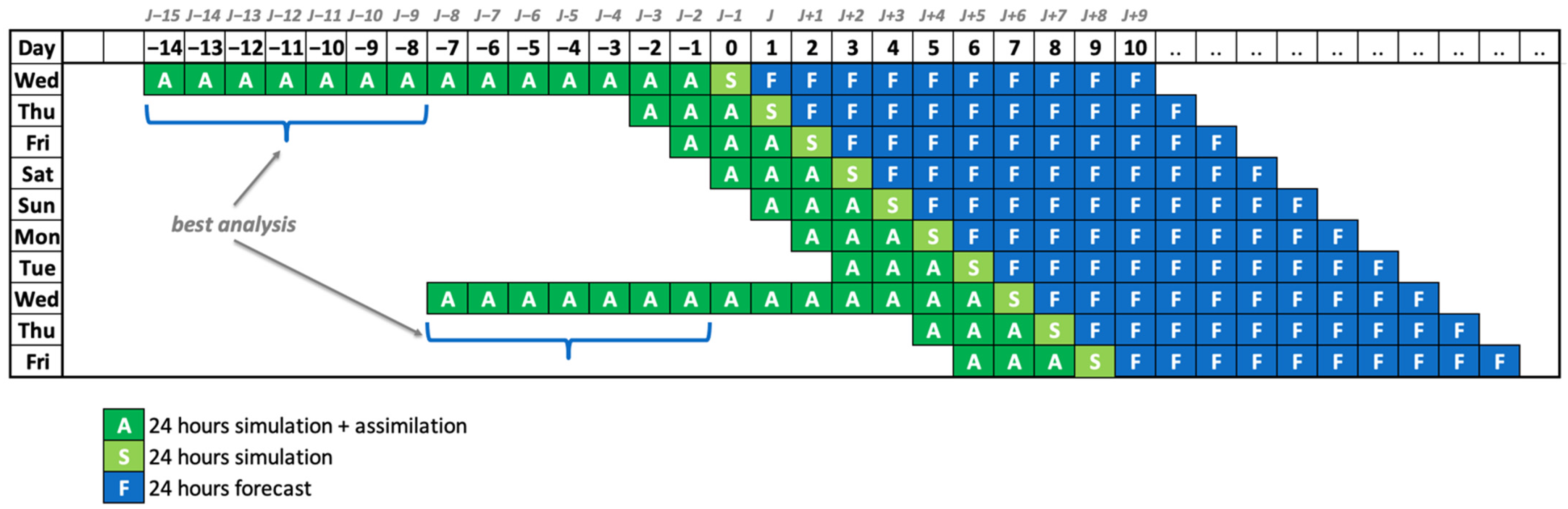
2.3. Operational Chain

BSFS version here considered is EAS3 (European Analysis and forecasting System, version 3, referred also in the next sections) for the Black Sea. It implements technical interfaces with upstream data, used for model runs—including ECMWF atmospheric forcing, CMEMS in-situ and satellite observations from corresponding TACs—as well as with the CMEMS Dissemination Unit for the delivery of analysis and forecast products to users. Observations used by BSFS for assimilation and validation are summarized in

Table 1. List of observations used by BSFS in the assimilation and verification steps.

Product Reference	Platforms/Satellite	Upstream Reference	Usage
Temperature and Salinity profiles	ARGO	INSITU_BS_NRT_ OBSERVATIONS_013_034	Validation, Assimilation
Sea Surface Temperature (SST)	SLSTR and AVHRR on Sentinel-3A and 3B, and NOAA, VIIRS, MetOp-B, MODIS AQUA, TERRA and SEVIRI on board of MSG satellite	SST_BS_SST_L4_NRT_OBSERVATIONS_010_006	Assimilation
		SST_BS_SST_L3S_NRT_OBSERVATIONS_010_013	Validation
Along track Sea Level Anomaly (SLA)	Altika Cryosat-2 H2B Jason-2 Jason-3 Sentinel-3A Sentinel-3B	SEALEVEL_EUR_PHY_L3_NRT_ OBSERVATIONS_008_059 from CMEMS	Validation, Assimilation

.

The atmospheric forcing (previous day analyses and 10 days forecast starting at 00:00 UTC) is downloaded from ECMWF through Aeronautica Militare Italiana. As soon as it is available, the BSFS processing system starts (at around 7:00 UTC). The atmospheric forcing availability is a major source of delay for the oceanic forecast.

Every day the BSFS (Figure 1) produces ten days of forecast (J to J+9), one day of simulation (J−), and three days of analysis (J−4 to J−1). Once a week (on Tuesday), 14 days of analysis are produced, from J−15 to J−1, with the assimilation of all available satellite and in-situ data collected over the past weeks. Analysis produced at the weekly cycle represents the best estimation of the Black Sea state because all in-situ and satellite altimetry high quality processing data is used up to J−3. Analysis and simulation runs are forced by ECMWF atmospheric analysis fields at 6 h frequency; the forecast cycle is forced with ECMWF atmospheric forecast fields at 3 h frequency for the first 3 days and 6 h frequency for the remaining 7 days.

At the end of the forecasting cycle, post-processing involves the preparation of all the BSFS files in a format that is compliant with the CMEMS and CF standards, delivering to the CMEMS DU, and archiving of the BSFS native products at CMCC’s supercomputing facilities. Every day, the forecast is released to CMEMS within less than 3 h (target delivery time: 12 UTC).

The BSFS product catalogue includes daily and hourly mean datasets, centered at midday of each J, for the Black Sea essential variables: 3D temperature (T), salinity (S), zonal and meridional velocity components (U and V, respectively) and 2D sea surface height (SSH), bottom temperature (BottomT) and mixed layer depth (MLD).

The BSFS operational chain is very similar to that of the Mediterranean Forecasting System (MFS, [25]) in terms of general setup (technical interface, analysis-simulation-forecast chain). Unlike MFS, it implements a more frequent analysis cycle to provide higher quality Black Sea products using daily observations.

3. Quality Assessment of the Operational System

The aim of the product quality assessment is to monitor the analysis quality and forecast accuracy of BSFS products using quasi-independent validation assessment. Operationally, a regional website provides daily bulletins (http://bsfs.cmcc.it/, accessed on 29 December 2021) and skill scores (http://oceanlab.cmcc.it/bsfs-evaluation/, accessed on 29 December 2021). Daily bulletins consist of a collection of interactive 2D maps for visualizing the essential variables of the Black Sea (as provided in the CMEMS catalogue). Weekly skill scores are provided through the evaluation section: during the assimilation weekly cycle, as described in Section 2.3, the difference between the model analysis and the observations at the time and location of the observations (i.e., misfits) is stored to compute statistics. Two main statistical metrics for the assessment of the analysis quality are computed using the misfits: the first is the bias, given by:

$$\mathrm{bias}\left(\varphi \right)=\frac{1}{N}{\displaystyle \sum }\left({\varphi }_i^M-{\varphi }_i^O\right)$$

(13)

and the Root Mean Square Error (RMSE) given by:

$$\mathrm{RMSE}\left(\varphi \right)=\sqrt{\frac{1}{N}{\displaystyle \sum }_{i=1}^N{\left({\varphi }_i^M-{\varphi }_i^O\right)}^2}$$

(14)

where $N$ is the number of data used in the evaluation, ${\varphi }_{}^M$ is the model analysis field, and ${\varphi }_{}^O$ the observation.

On the other hand, to assess the quality of the forecast, we evaluated the differences of the forecast fields with respect to the analysis considered to be the best estimate of the truth. Murphy (1993, [26]), revisited by [2], defined the “forecast goodness” methodology and here we use his “quality measure” methodology that compares the forecast with the analysis and the “persistence” or the best estimate at initial time. If the difference between forecast and analysis is better than the difference between forecast and persistence, then the forecast is valuable. For a modern oceanographic forecasting system, [27] defined a metrics that we will partially follow here by computing:

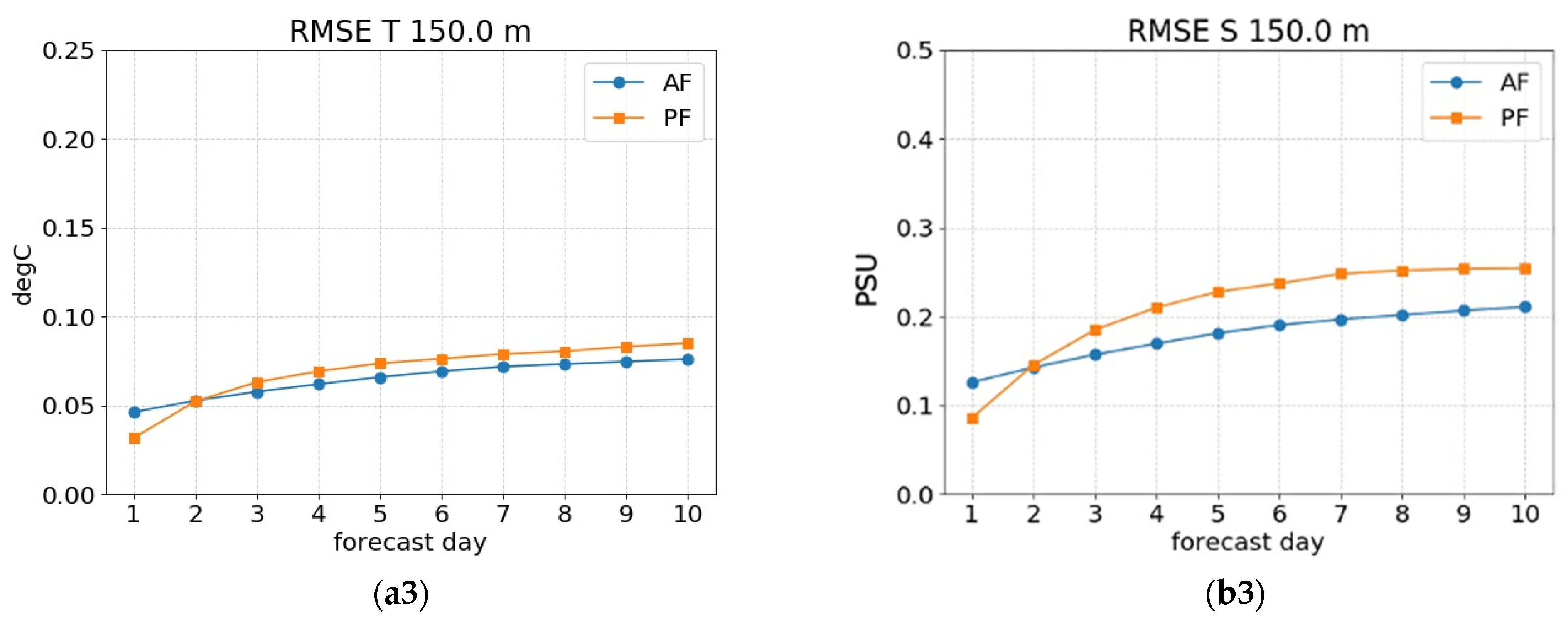
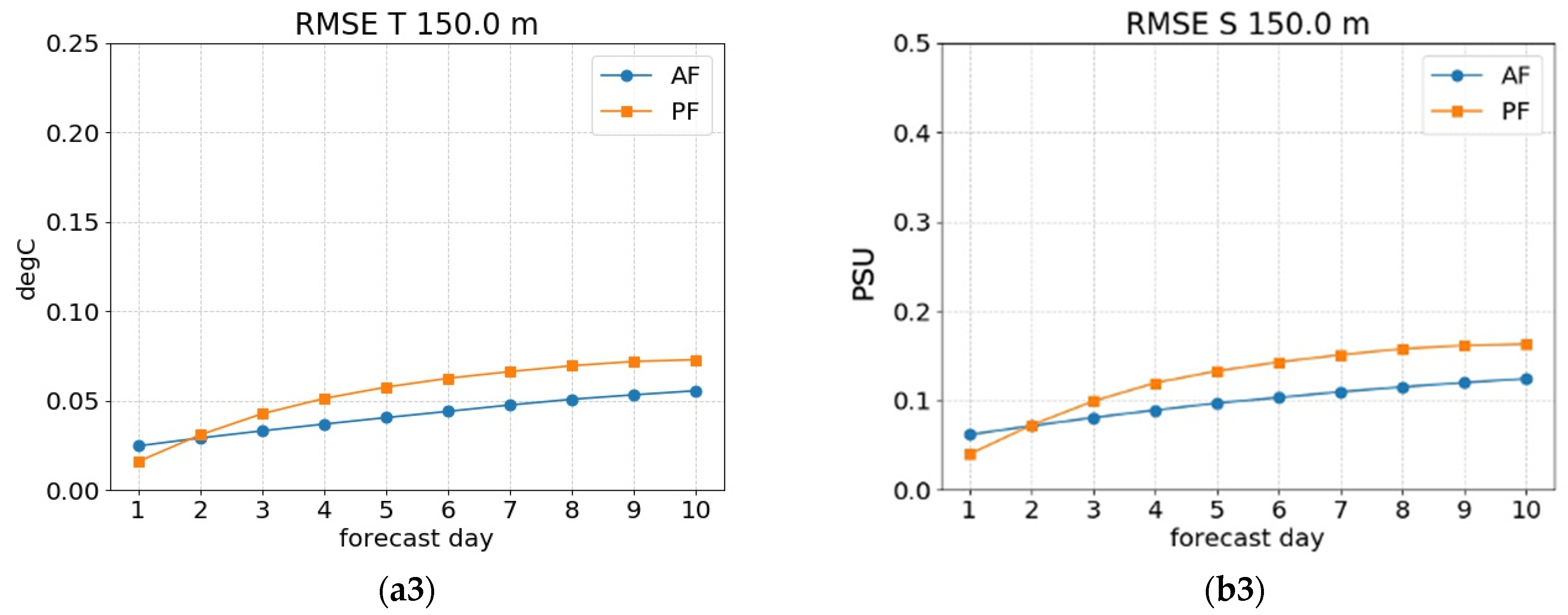
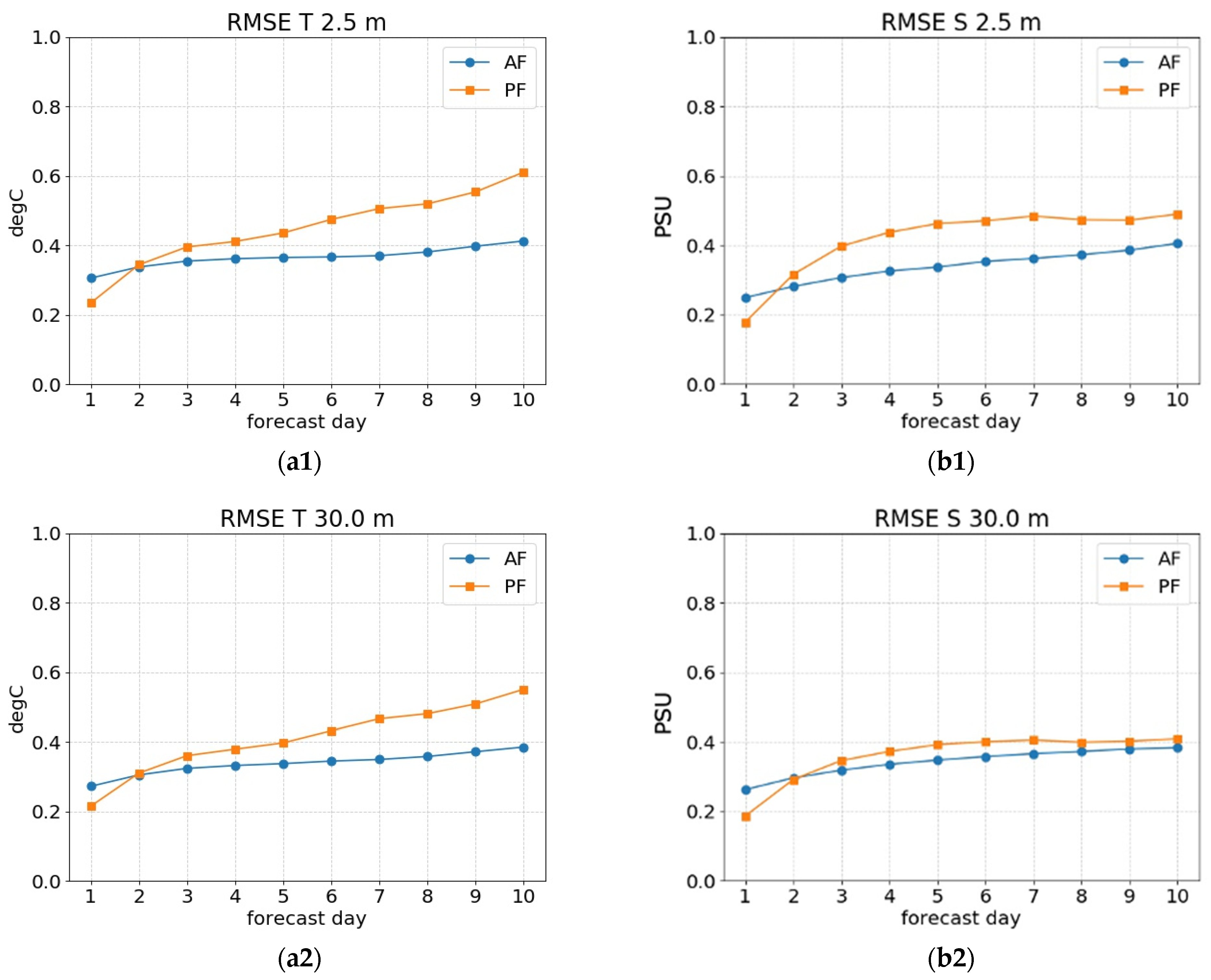
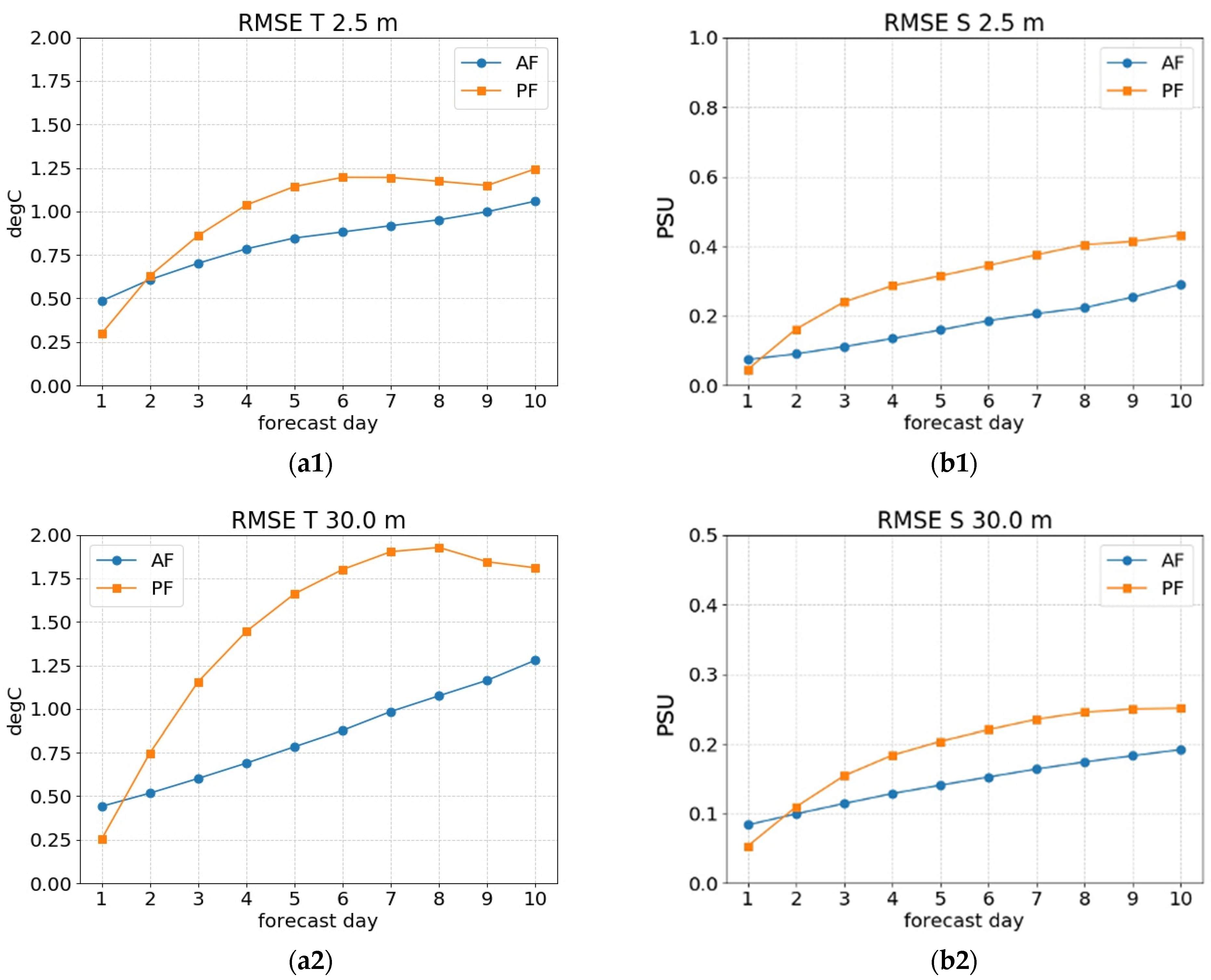
• The difference between the analysis and the forecast (AF):

$$AF\left(t\right)=\sqrt{\frac{{{\displaystyle \sum }}_1^T{\left({\varphi }_{}^{AN}\left(t\right)-{\varphi }_{}^{FC}\left(t\right)\right)}^2}{T}}$$

(15)

where ${\varphi }_{}^{AN}$ and ${\varphi }_{}^{FC}$ is the temperature (salinity) daily mean forecast and analysis, respectively, at each forecast day $t=day1, day2, \dots , day10$ (ID day as in Figure 2); $T$ corresponds to the time period covered by the evaluation (here we consider a time period of 1 month). The metrics is normalized horizontally by averaging over the area and at a specific selected depth.

• The difference between the forecast and the persistence (PF):

$$PF\left(t\right)=\langle \sqrt{\frac{{{\displaystyle \sum }}_1^N{\left({\varphi }_{}^{FC}\left(t\right)-{\varphi }_{}^{AN}\left(t=day0\right)\right)}^2}{N}}\rangle$$

(16)

Here, ${\varphi }_{}^{AN}\left(t=day0\right)$ is the persistence (ID day as in Figure 2), e.g., the initial condition for the forecast. The latter is the last time step of a simulation started from an assimilated initial condition at day J−2.

In the following subsections, we present BSFS analysis statistics for the period 2018–2019 for SST and SLA, as well as temperature and salinity at given layers: 2–5 m, 5–10 m, 10–20 m, 20–30 m, 30–50 m, 50–75 m, 75–100 m, 100–200 m, 200–500 m, and 500–1000 m. Forecast assessment is performed for 2 significant months—February and August 2020: metrics have been computed at selected depth, e.g., 2.5, 30, 150 m.

3.1. Sea Surface Temperature

The BSFS analysis sea surface temperature is assessed by comparing analysis model fields against SST satellite data remapped over the Black Sea basin at 1/16° spatial resolution and representative of night SST values and delivered by CMEMS (Table 1).

Figure 3 shows the time series from 2018 to 2019 of the difference between BSFS and satellite SST (BIAS, top) and RMSE (bottom). The numerical SST is slightly warmer than the measured one (+0.1 °C), and the error is about 0.5 °C.

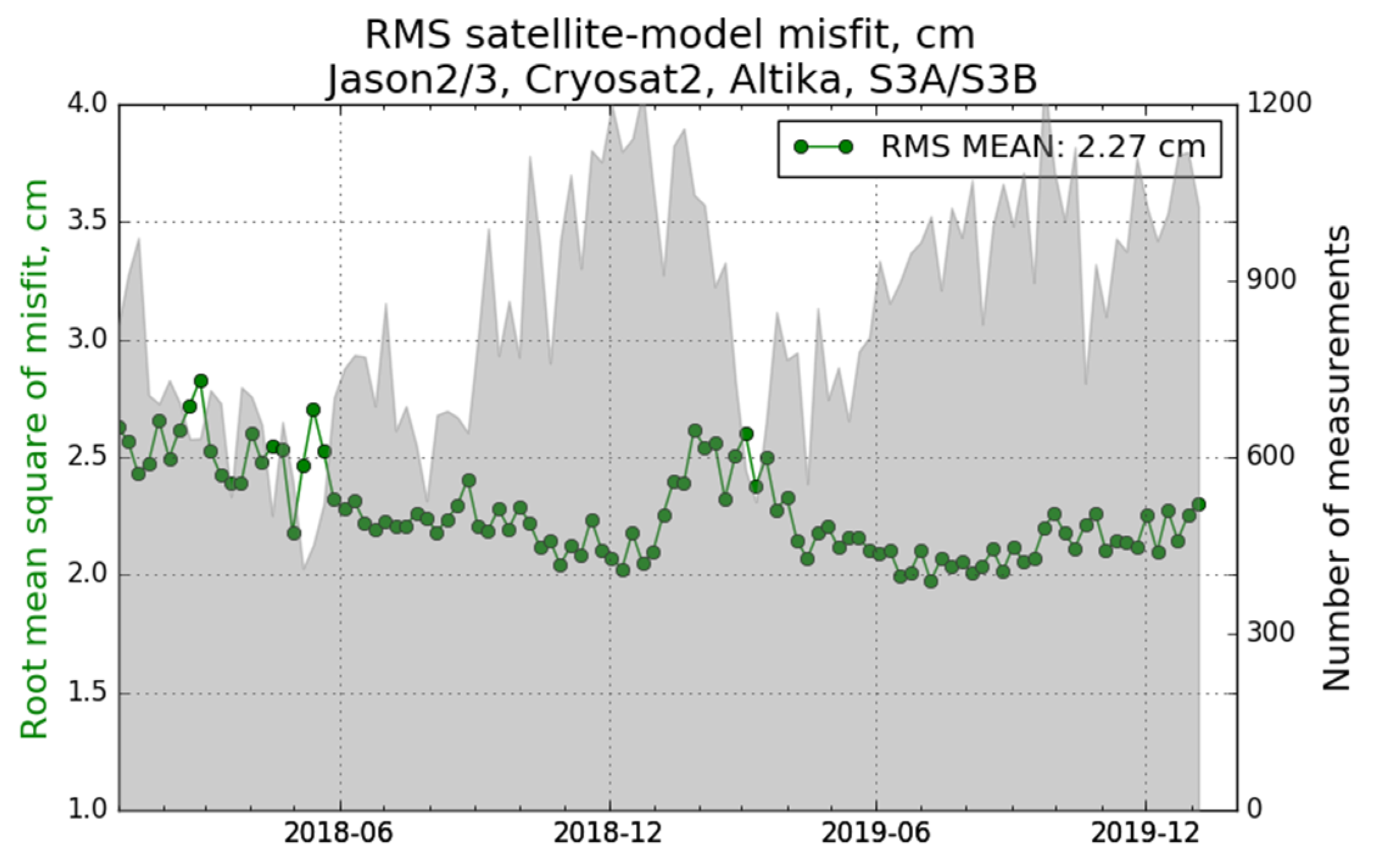
3.2. Sea Surface Height

Figure 4 shows the RMSE for SLA in the operational period (green dotted line) and the number of observational data used, given by the sum of the available along track sea level data provided by Altika, Cryosat-2, Jason-2 and 3, Sentinel 3A and 3B. The mean value of RMSE misfits for SLA is around 2.3 cm. A decrease in the error is also shown once the number of observations increases (June 2018–December 2018; March 2019–October 2019 thanks to inclusion of Sentinel-3B data). The accuracy is comparable to the Mediterranean Sea [25], where the average error over the same period is about 3.35 cm (http://oceanlab.cmcc.it/mfs-evaluation/ accessed on 29 December 2021).

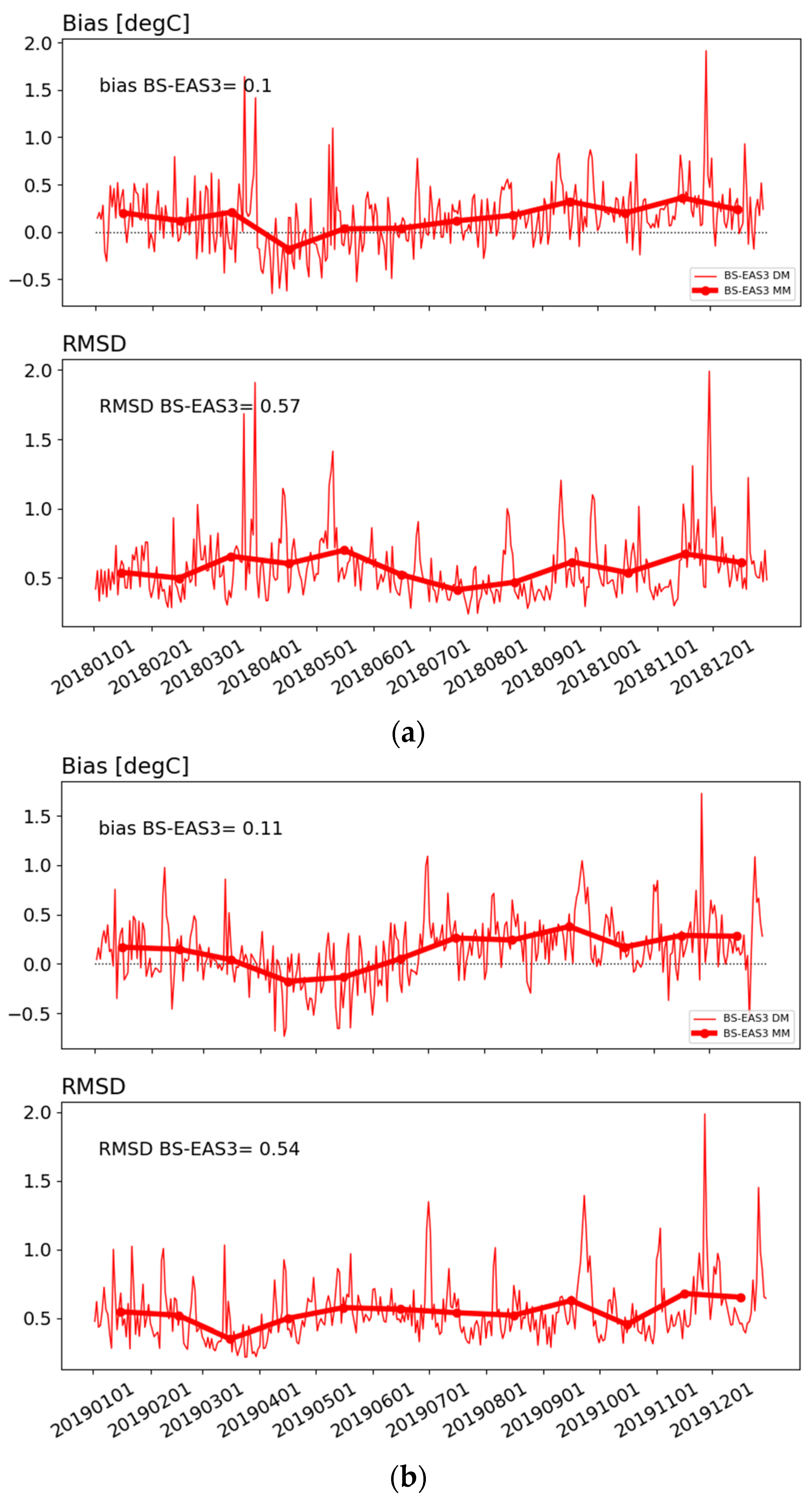
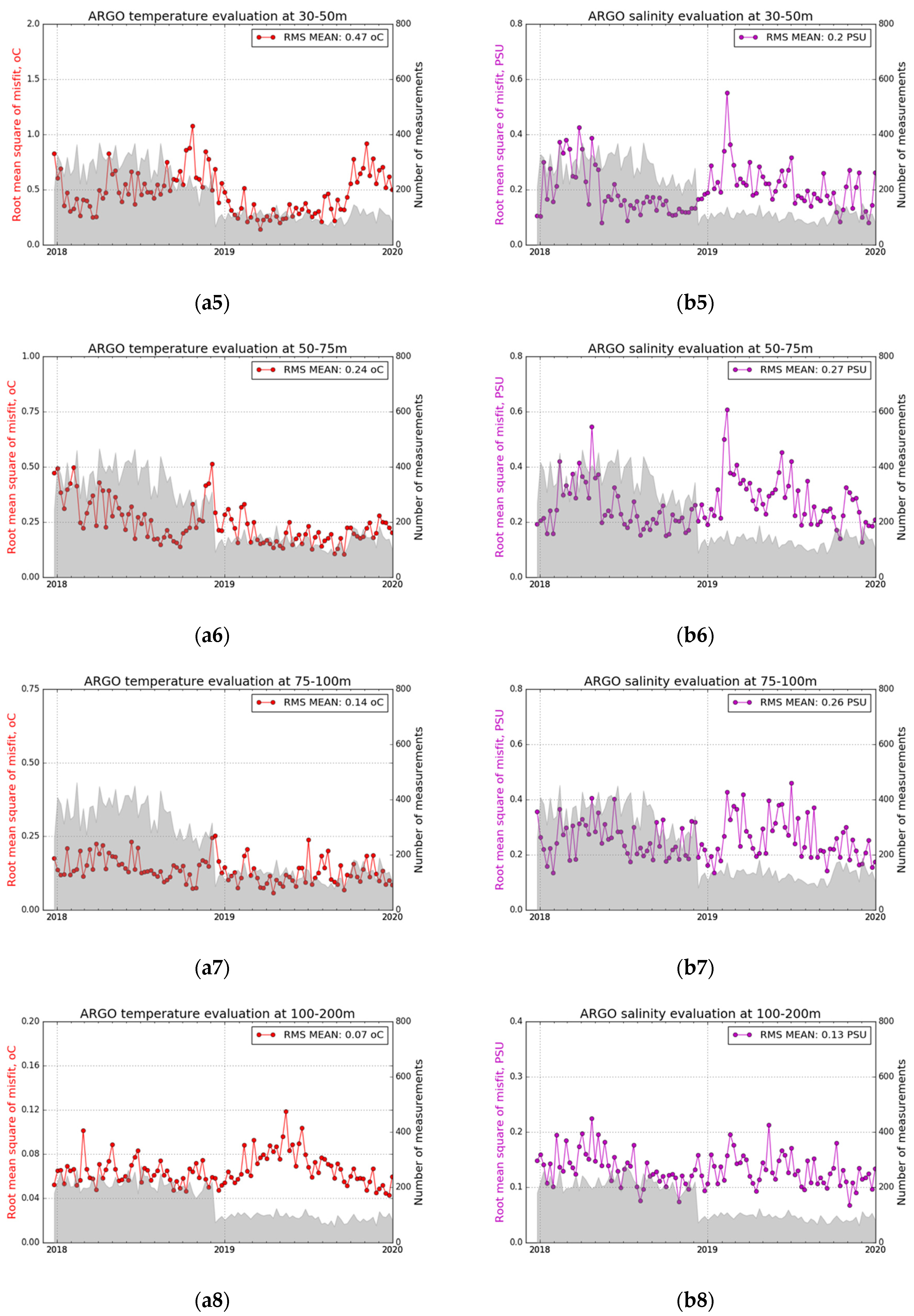
3.3. Temperature and Salinity

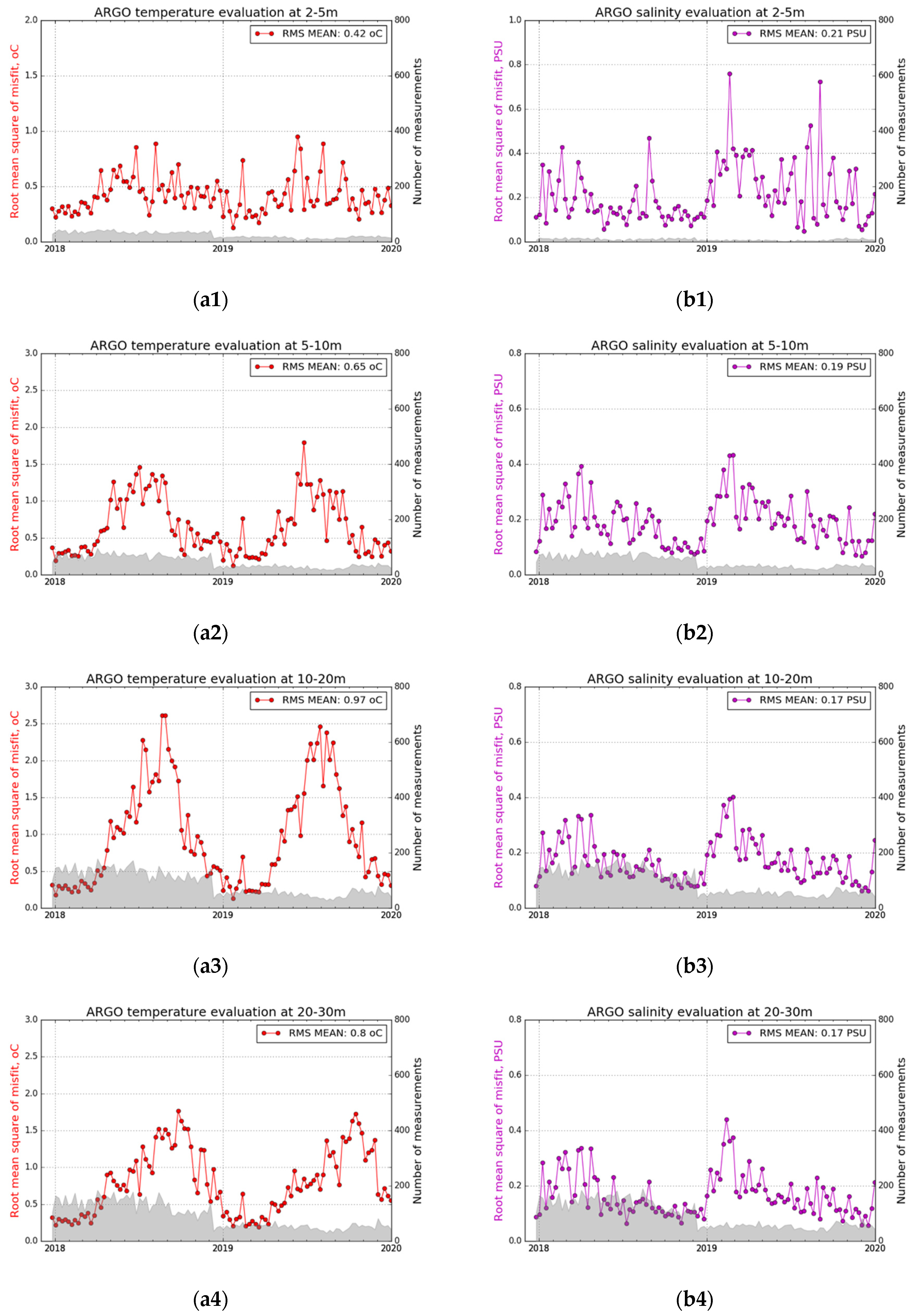
3.3.1. Analysis Quality

Water column properties given by BSFS are assessed after 3D temperature and salinity are validated against all available observations.

Table 2. Temperature and salinity RMSE misfits over the period 2018–2019.

Layer (m)	T RMSE Misfit (°C)	S RMSD Misfit (PSU)
2–5	0.42	0.21
5–10	0.65	0.19
10–20	0.97	0.17
20–30	0.80	0.17
30–50	0.47	0.20
50–75	0.24	0.27
75–100	0.14	0.26
100–200	0.07	0.13
200–500	0.02	0.05

shows the basin scale RMSE misfits at specific layers (m) for 2018–2019. In the 2–5 m surface layer, the average RMSE for temperature at the whole basin is about 0.4 °C (Figure 5(a1)) and 0.2 PSU (Figure 5(b1)). However, the error in temperature starts to increase in the sub-surface, from 5 m to 30 m, from 0.5 °C to 2 °C in the summer and below 0.5 °C in the winter (Figure 5(a2–a4)).

The maximum error for temperature occurs in the 10–20 m layer with a value up to 2.5 °C computed for August–October in both 2018 and 2019 (Figure 5(a3)).

Regarding salinity, the error in the subsurface, on average, is around 0.2 PSU (Figure 5(b2–b4)), which increases from 30 m up to 100 m up to a maximum value of 0.4 PSU (Figure 5(b5–b7)). In the intermediate layers up to 1000 m, the error decreases to quasi-zero for both temperature (Figure 5(a8)) and salinity (Figure 5(b8)).

The increased error in the thermocline (10–30 m layer) and in the halocline (50–100 m layer) in the summer is likely due to a deficiency in the vertical discretization (we use only 31 z-levels) and in the vertical mixing parameterization.

The errors are due to (a) the Bosporus Strait being represented as closed boundary, (b) mixing processes that were not completely resolved since effects induced by waves and tides are not accounted for, and (c) simplified representation of the heat, momentum and water fluxes through bulk formulation, whose effects are particularly important especially during the summer. These are significant challenges to be considered in the development of the next generation of the Black Sea physical system.

3.3.2. Forecast Assessment

In Figure 6 and Figure 7 we present the BSFS forecast quality assessment for temperature and salinity considering 2 reference months, February 2020 and August 2020, respectively. Metrics are given at different depths—2.5, 30 and 150 m. If the forecast is skillful, $AF$ score should be better than $PF$ score.

In February 2020, $PF$ is bigger than $AF$ after $day2$ (Figure 6 and Figure 7): this means that after the first day the advantage of doing the forecast is clear over persisting the initial condition. It is interesting to note that for salinity this advantage grows more rapidly, i.e., for salinity the forecast overcomes the persistence even before the first day. Over the water column, temperature and salinity analysis and forecast exhibit a similar variability: higher error reaching a maximum around 0.6° Celsius and 0.5 PSU at $day10$ is shown for temperature (Figure 6(a1,a2)) and salinity (Figure 6(b1,b2)) in the subsurface up to 30 m; at 150 m, both variables exhibit a lower error (never higher than 0.1° Celsius and 0.3 PSU over the reference 10-day period).

In August 2020, errors at 30 m are higher than the ones computed in the previous analyzed month: starting from $day2,$ in particular for temperature (Figure 7(a1,a2)), $PF$ shows higher values than $AF$—almost 50% higher at 30 m, with maximum error of about 2.0° Celsius (Figure 7(a2)). This means that during the summer the forecast adds to persistence more than during winter: the dynamical model is clearly responsible for the proper changes in water column stratification even for few days. At 30 m and in August (Figure 7(a1)) the difference between $PF$ and $AF$ is the largest: we assume that this is an indication of the complex dynamics involved in the mixing and the CIL dynamics. Regarding salinity (Figure 7(b1–b3)), $PF$ and $AF$ errors are quite similar comparing to winter and of the order of 0.3–0.4 PSU.

4. Black Sea Diagnostics and Circulation Consistency

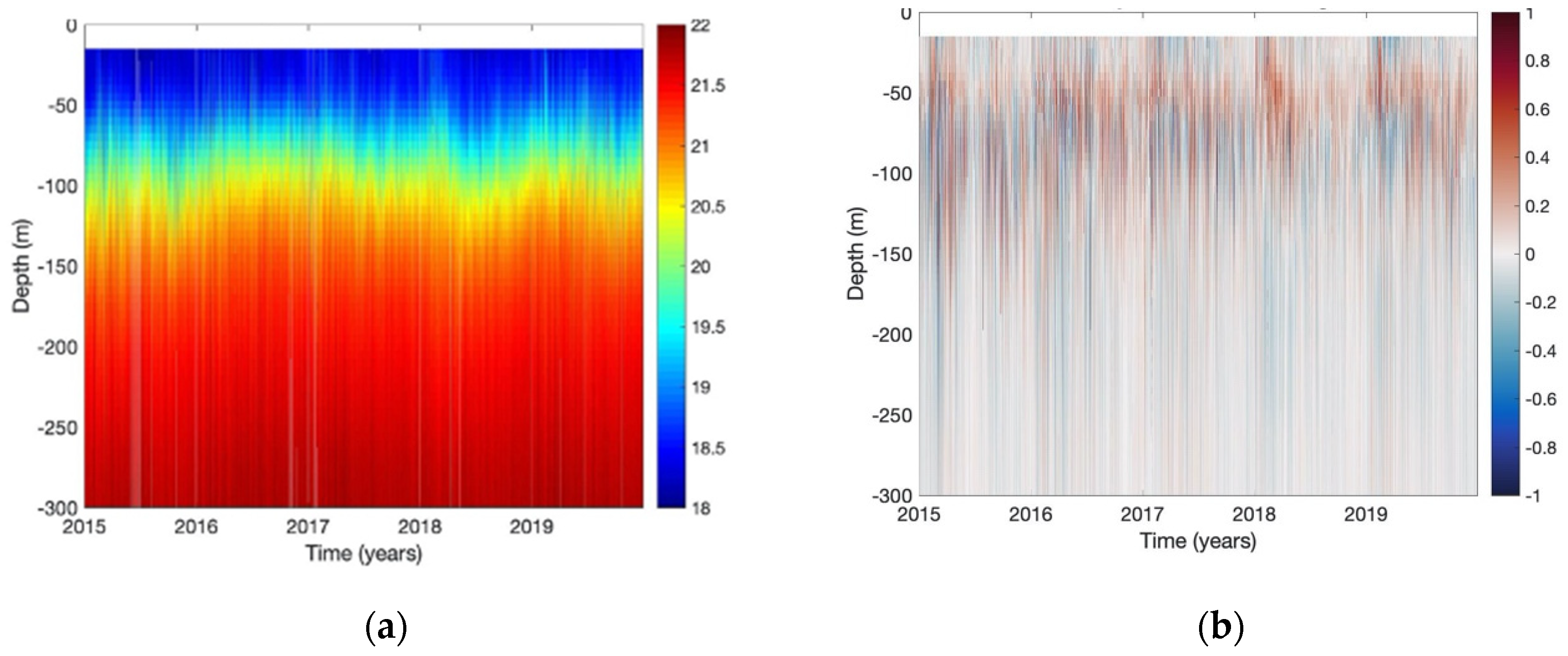
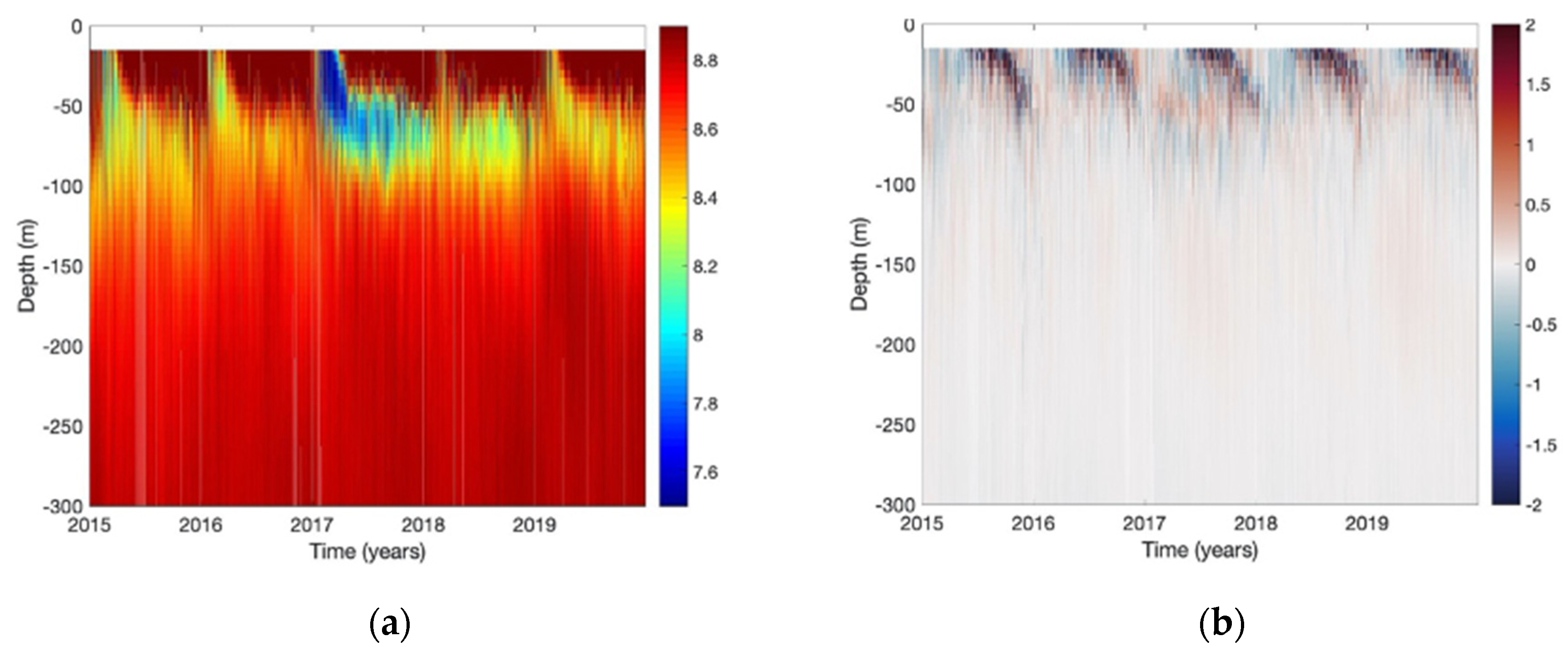
4.1. Temporal Evolution of the CIL and Stratification

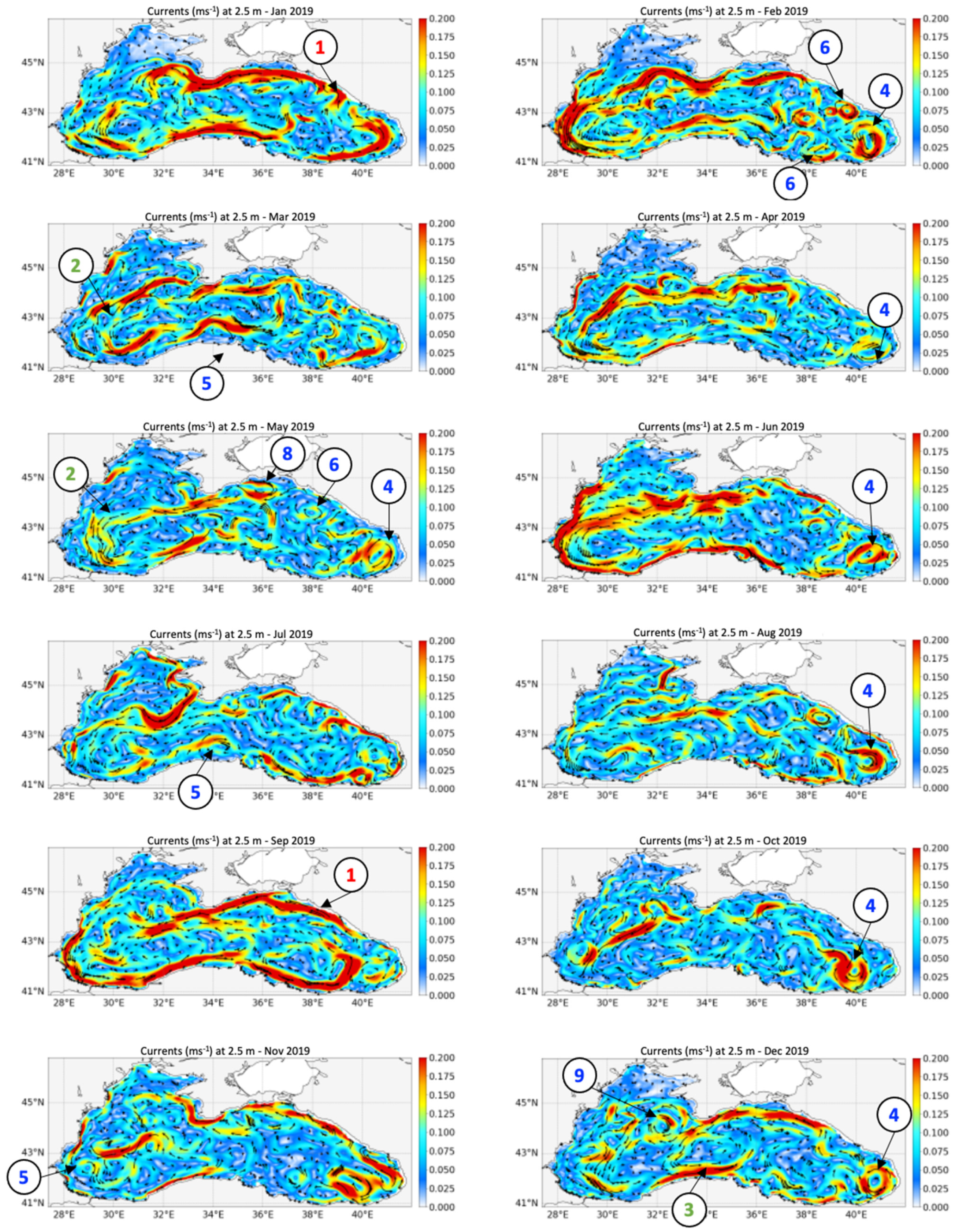
The BSFS is able to represent the formation and evolution of the cold intermediate layer (CIL), which is a typical water mass property of the Black Sea basin, and well documented in the literature ([16] for a very comprehensive literature review and updated evaluation). It is identified by the 8.0 °C isotherm, arising at the surface during winter, penetrating the subsurface (typically at a depth range of 50–100 m), intruding the warmer zone, and persisting over time. The time versus depth diagrams at the observation location are shown for temperature and for salinity in Figure 8, between 2015–2019. Figure 8a shows the cold event of 2017, which is also captured by observations as demonstrated by the quite low difference between the model and observations (Figure 8b). It also shows the reduction in the CIL width because of the warming period from 2018 and its perforation and partial disappearance in 2019 [16]. The major differences of about 2 °C occur in the upper layer and are shown in Figure 8b. Salinity stratification is well represented in Figure 9a with small differences with respect to observations, as shown in Figure 9b. It is characterized by a 2-layer structure with low salt in the CIL zone down to 100 m in depth and saltier values of about 22 PSU or more in the intermediate to deepest levels.

4.2. Circulation

The surface mean circulation is shown in Figure 10 as monthly means for 2019. Considering the poor availability of observations, a robust validation exercise is extremely difficult, thus the main features emerging from the annual monthly means are described in detail with respect to those extensively described in [28,29,30,31].

The Black Sea surface dynamics is characterized by a main cyclonic gyre, the Rim current, encompassing the basin and a variety of mesoscale eddies along the coast, some of them quasi-stationary. BSFS captures most of the particular dynamical structures in the basin, such as the Rim current, which persists over 2019, and small-scale structures such as coastal anticyclonic eddies, which appear along the Russian–Georgian coastline (one quite intense in February and progressively weaker in March) and coastal cyclonic eddies, which are much more intermittent over the year and weak). The Batumi Gyre, located near the Georgian coast, forms in April and lasts until June, when the circulation in that region is fragmented in more unstable and weak eddies until its regeneration in August–September. Progressively towards the southwestern region, small coastal eddies become part of the Rim current. On the Turkish coastline, cyclonic eddies like the one in the area of Trabzon (January–February; November–December) coexist with anticyclonic eddies, as in the Synop area (June–October). In the area between Istanbul and Burgas—the Bosporus region—an anticyclonic eddy appears from October to December. Close to the Danube, coastal currents are quite well captured by the model, then going further towards the continental slope (30° E–32° E and 44° N–45° N) the Sevastopol anticyclonic gyre starts in May (very weak), becoming stronger in November and December.

5. Conclusions

Within the framework of the CMEMS and the BS-MFC, the Black Sea physical analysis and forecasting system provides essential variables for understanding the physical processes and dynamics of the Black Sea basin. The BSFS has been operational since the end of 2016 and has been developed and maintained at CMCC in collaboration with the USOF (University of Sofia, Bulgaria, scientific partner in the BS-MFC consortium).

We have presented the BSFS ocean model based on NEMO v3.4 able to assimilate near real time, in-situ and satellite observational products using the OceanVar scheme. The Black Sea hydrodynamic model has about 3 km horizontal resolution and uses 31 levels with partial steps. It implements a closed boundary condition at the Bosporus Strait and is forced by ECMWF analysis and forecasting atmospheric fields.

The BSFS implements two production cycles, one daily (which includes 3 days analysis) and one weekly (based on 14 days analysis), the latter to assimilate a higher number of collected observations to provide the best quality initial conditions for the forecasting cycle: the processing system is completed every day by 1-day simulation and 10-day forecasts.

We have also described an operational dashboard for product quality monitoring which assesses the skill scores of the analysis products for 2018–2019 and gives an accuracy of around 1 °C in the sea surface temperature. Errors increase at the sub-surface (10–30 m layer): in particular, the thermocline experiences a maximum error of 2 °C during the summer period, while salinity reaches an error of about 0.5 PSU. Considering the sea level, the assimilation of the along-track satellite SLA guarantees an average error of about 2.3 cm. Such skills put the BSFS on the same track of quality and robustness as state-of-the-art regional configurations in the CMEMS framework. A regional website is operationally maintained at CMCC to provide daily bulletins and metrics for monitoring the lifecycle and performances of the system.

The future forecasting system for the Black Sea will include at least four new main components which will significantly improve the quality of the BSFS analysis fields and forecasting skill scores by means of improved hydrodynamical core model: (1) increased vertical resolution for a better representation of open ocean dynamics and mixing processes, combined with a revised bathymetry and coastline and data assimilation upgrades; (2) the Bosporus Strait will work as an open boundary, in order to improve the connection with the Mediterranean Sea. This will be achieved thanks to a novel implementation of the Marmara Sea model, based on an unstructured grid method that provides open boundary conditions to the Black Sea through the Bosporus and the Mediterranean Sea through the Dardanelles; (3) improved representation of the land forcing: in particular, the representation of the Danube River using historical discharge datasets provided by the NIHWM (National Institute of Hydrology and Water Management, Romania—scientific partner in the BS-MFC consortium); (4) an online wave-current model to improve the small scales dynamics at the surface.

References

1. Pinardi, N.; Cavaleri, L.; Coppini, G.; De Mey, P.; Fratianni, C.; Huthnance, J.; Lermusiaux, P.F.J.; Navarra, A.; Preller, R.; Tibaldi, S. From weather to ocean predictions: An historical viewpoint. J. Mar. Res. 2017, 75, 103–159. [Google Scholar] [CrossRef] [Green Version]
2. Brassington, G.B. Forecast Terrors, goodness and verification in Ocean forecasting. J. Mar. Res. 2017, 75, 403–433. [Google Scholar] [CrossRef]
3. Le Traon, P.Y.; Reppucci, A.; Alvarez Fanjul, E.; Aouf, L.; Behrens, A.; Belmonte, M.; Bentamy, A.; Bertino, L.; Brando, V.E.; Kreiner, M.B.; et al. From Observation to Information and Users: The Copernicus Marine Service Perspective. Front. Mar. Sci. 2019, 6, 234. [Google Scholar] [CrossRef] [Green Version]
4. Pinardi, N.; Coppini, G. Operational oceanography in the Mediterranean Sea: The second stage of development. Ocean Sci. 2010, 6, 263–267. [Google Scholar] [CrossRef] [Green Version]
5. Clementi, E.; Oddo, P.; Drudi, M.; Pinardi, N.; Korres, G.; Grandi, A. Coupling hydrodynamic and wave models: First step and sensitivity experiments in the Mediterranean Sea. Ocean. Dyn. 2017, 67, 1293–1312. [Google Scholar] [CrossRef] [Green Version]
6. Palazov, A.; Ciliberti, S.A.; Peneva, E.; Gregoire, M.; Staneva, J.; Lemieux-Dudon, B.; Masina, S.; Pinardi, N.; Vandenbulcke, L.; Behrens, A.; et al. Black Sea Observing System. Front. Mar. Sci. 2019, 6, 1–8. [Google Scholar] [CrossRef]
7. Madec, G.; The NEMO Team. NEMO Ocean Engine, Note du Pôle de Modélisation; Institute Pierre-Simon Laplace (IPSL): Paris, France, 2008; ISSN 1288–1619. [Google Scholar]
8. Stanev, E.V.; Rachev, N.H. Numerical study on the planetary Rossby waves in the Black Sea. J. Mar. Syst. 1999, 21, 283–306. [Google Scholar] [CrossRef]
9. Historical GEBCO Data Sets. Available online: https://www.gebco.net/data_and_products/historical_data_sets/#gebco_one (accessed on 1 April 2021).
10. Wessel, P.; Smith, W.H.G. A global, self-consistent, hierarchical, high-resolution shoreline database. J. Geophys. Res. 1996, 101, 8741–8743. [Google Scholar] [CrossRef] [Green Version]
11. Pettenuzzo, D.; Large, W.G.; Pinardi, N. On the corrections of ERA-40 surface flux products consistent with the Mediterranean heat and water budgets and the connection between basin surface total heat flux and NAO. J. Geophys. Res. 2010, 115, C06022. [Google Scholar] [CrossRef]
12. Roullet, G.; Madec, G. Salt conservation, free surface, and varying levels: A new formulation for ocean general circulation models. J. Geophys. Res. 2000, 105, 23927–23942. [Google Scholar] [CrossRef]
13. Jarosz, E.; Teague, W.J.; Book, J.W.; Beşiktepe, Ş. On flow variability in the Bosphorus Strait. J. Geophys. Res. 2011, 116, C08038. [Google Scholar] [CrossRef] [Green Version]
14. Özsoy, E.; Altıok, H.A. Review of Hydrography of the Turkish Straits System. In The Sea of Marmara-Marine Biodiversity, Fisheries, Conservation and Governance; Özsoy, E., Çağatay, N.M., Balkis, N., Öztürk, B., Eds.; Turkish Marine Research Foundation (TÜDAV): Istanbul, Turkey, 2016; Publication #42. [Google Scholar]
15. Özsoy, E.; Çağatay, N.M.; Balkis, N.; Öztürk, B. Review of Water Fluxes across the Turkish Straits System. In The Sea of Marmara-Marine Biodiversity, Fisheries, Conservation and Governance; Özsoy, E., Altiok, H., Eds.; Turkish Marine Research Foundation (TÜDAV): Istanbul, Turkey, 2016; Publication #42. [Google Scholar]
16. Stanev, E.V.; Peneva, E.; Chtirkova, B. Climate change and regional ocean water mass disappearance: Case of the Black Sea. J. Geophys. Res. 2019, 124, 4803–4819. [Google Scholar] [CrossRef]
17. Ünlüata, Ü.; Oğuz, T.; Latif, M.A.; Özsoy, E. On the physical oceanography of the Turkish Straits. In The Physical Oceanography of Sea Straits; NATO/ASI Series; Kluwer: Dordrecht, The Netherlands, 1990; pp. 25–60. [Google Scholar]
18. Kara, A.B.; Wallcraft, A.J.; Hurlburt, H.E.; Stanev, E.V. Airsea fluxes and river discharges in the Black Sea with a focus on the Danube and Bosphorus. J. Mar. Syst. 2008, 74, 74–95. [Google Scholar] [CrossRef]
19. Pinardi, N.; Bonaduce, A.; Navarra, A.; Dobricic, S.; Oddo, P. The mean sea level equation and its application to the Mediterranean Sea. J. Clim. 2014, 27, 442–447. [Google Scholar] [CrossRef]
20. Stanev, E.V.; Beckers, J.M. Barotropic and baroclinic oscillations in strongly stratified ocean basins. Numerical study for the Black Sea. J. Mar. Syst. 1999, 19, 65–112. [Google Scholar] [CrossRef]
21. Ludwig, W.; Dumont, E.; Meybeck, M.; Heussner, S. River discharges of water and nutrients to the Mediterranean Sea: Major drivers for ecosystem changes during past and future decades? Prog. Oceanogr. 2009, 80, 199–217. [Google Scholar] [CrossRef]
22. Dobricic, S.; Pinardi, N. An oceanographic three-dimensional variational data assimilation scheme. Ocean Model. 2008, 22, 89–105. [Google Scholar] [CrossRef]
23. Storto, A.; Dobricic, S.; Masina, S.; Di Pietro, P. Assimilating along-track altimetric observations through local hydrostatic adjustment in a global ocean variational assimilation system. Mon. Weather Rev. 2010, 139, 738–754. [Google Scholar] [CrossRef] [Green Version]
24. Waters, J.; Lea, D.J.; Martin, M.J.; Mirouze, I.; While, J. Implementing a variational data assimilation system in an operational 1/4 degree global ocean model. Q. J. R. Meteorol. 2014, 141, 333–349. [Google Scholar] [CrossRef]
25. Clementi, E.; Pistoia, J.; Escudier, R.; Delrosso, D.; Drudi, M.; Grandi, A.; Lecci, R.; Cretí, S.; Ciliberti, S.; Coppini, G.; et al. Mediterranean Sea Analysis and Forecast (CMEMS MED-Currents, EAS5 System) [Data Set]; Copernicus Monitoring Environment Marine Service (CMEMS); Centro Euro-Mediterraneo sui Cambiamenti Climatici (CMCC): Lecce, Italy, 2019; Available online: https://doi.org/10.25423/CMCC/MEDSEA_ANALYSIS_FORECAST_PHY_006_013_EAS5 (accessed on 9 December 2021).
26. Murphy, A.H. What is a good forecast? An essay on the nature of goodness in weather forecasting. Weather Forecast. 1993, 8, 281–293. [Google Scholar] [CrossRef] [Green Version]
27. Tonani, M.; Pinardi, N.; Fratianni, C.; Pistoia, J.; Dobricic, S.; Pensieri, S.; de Alfonso, M.; Nittis, K. Mediterranean Forecasting System: Forecast and analysis assessment through skill scores. Ocean Sci. 2009, 5, 649–660. [Google Scholar] [CrossRef] [Green Version]
28. Ciliberti, S.A.; Peneva, E.L.; Jansen, E.; Martins, D.; Cretí, S.; Stefanizzi, L.; Lecci, R.; Palermo, F.; Daryabor, F.; Lima, L.; et al. Black Sea Analysis and Forecast (CMEMS BS-Currents, EAS3 System) (Version 1) [Data Set]; Copernicus Monitoring Environment Marine Service (CMEMS); Centro Euro-Mediterraneo sui Cambiamenti Climatici (CMCC): Lecce, Italy, 2020; Available online: https://doi.org/10.25423/CMCC/BLKSEA_ANALYSIS_FORECAST_PHYS_007_001_EAS3 (accessed on 9 December 2021).
29. Özsoy, E.; Ünlüata, Ü. Oceanography of the Black Sea: A review of some recent results. Earth-Sci. Rev. 1997, 42, 231–272. [Google Scholar] [CrossRef]
30. Staneva, J.V.; Stanev, E.V. Oceanic response to atmospheric forcing derived from different climatic data sets. Intercomparison study for the Black Sea. Oceanol. Acta 1998, 21, 393–417. [Google Scholar] [CrossRef] [Green Version]
31. Gunduz, M.; Özsoy, E.; Hordoir, R. A model of Black Sea circulation with strait exchange (2008–2018). Geosci. Model Dev. 2020, 13, 121–138. [Google Scholar] [CrossRef] [Green Version]
32. Castellari, S.; Pinardi, N.; Leaman, K. A model study of air-sea interactions in the Mediterranean Sea. J. Mar. Syst. 1998, 18, 89–114. [Google Scholar] [CrossRef]
33. Reed, R.K. On estimating insolation over the ocean. J. Phys. Oceanogr. 1977, 7, 482–485. [Google Scholar] [CrossRef] [Green Version]
34. Payne, R.E. Albedo of the sea surface. J. Atmos. Sci. 1972, 29, 959–970. [Google Scholar] [CrossRef]
35. Rosati, A.; Miyakoda, K. A general circulation model for upper ocean simulation. J. Phys. Oceanogr. 1988, 18, 1601–1626. [Google Scholar] [CrossRef]
36. Lowe, P.R. An approximating polynomial for the computation of saturation vapor pressure. J. Appl. Meteorol. 1977, 16, 100–103. [Google Scholar] [CrossRef] [Green Version]
37. Bignami, F.; Marullo, S.; Santoleri, R.; Schiano, M.E. Long wave radiation budget on the Mediterranean Sea. J. Geophys. Res. 1995, 100, 2501–2514. [Google Scholar] [CrossRef]
38. Kondo, J. Air-sea bulk transfer coefficients in diabatic condition. Bound. Layer Meteorol. 1975, 9, 91–112. [Google Scholar] [CrossRef]
39. Hellerman, S.; Rosenstein, M. Normal monthly wind stress over the world ocean with error estimates. J. Phys. Oceanogr. 1983, 23, 1009–1039. [Google Scholar] [CrossRef] [Green Version]
Figure 1. BSFS spatial domain and bathymetry (expressed in meters, from 0 to −2200 m).
Jmse 10 00048 g001
Figure 2. BSFS processing chain.
Jmse 10 00048 g002
Figure 3. SST bias (top) and RMSE (bottom) timeseries, expressed in °C, at daily (thinner line) and monthly (solid line) frequency in 2018 (a) and 2019 (b).
Jmse 10 00048 g003
Figure 4. RMSE misfit of SLA, expressed in cm, computed using available observations from Altika, Cryosat-2, Jason-2 and 3, Sentinel-3A and 3B during 2018–2019.
Jmse 10 00048 g004
Figure 5. RMSE timeseries between BSFS analysis fields and ARGO observations for temperature (a1a8) (expressed in °C) and salinity (expressed in PSU) (b1b8). The reference layer as considered for the evaluation is written on the top of each panel.
Jmse 10 00048 g005aJmse 10 00048 g005b
Figure 6. RMSE of A F (Analysis-Forecast, in blue), P F (Forecast-Persistence, in orange) for temperature (on the left, (a1a3), expressed in °C) and salinity (on the right, (b1b3), expressed in PSU) at 2.5 m (1), 30.0 m (2) and 150 m (3), computed for February 2020.
Jmse 10 00048 g006aJmse 10 00048 g006b
Figure 7. RMS of A F (Analysis-Forecast, in blue), P F (Forecast-Persistence, in orange) for temperature (on the left, (a1a3), expressed in °C) and salinity (on the right, (b1b3), expressed in PSU) at 2.5 m (1), 30.0 m (2) and 150 m (3), computed for August 2020.
Jmse 10 00048 g007aJmse 10 00048 g007b
Figure 8. Time versus depth diagram for BSFS temperature in the period 2015–2019 (a) at the observation location and (b) for the computed model minus observation value.
Jmse 10 00048 g008
Figure 9. Time versus depth diagram for BSFS salinity (PSU) in the period 2015–2019 (a) at the observation location and (b) for the computed model minus observation value.
Jmse 10 00048 g009
Figure 10. Surface currents in 2019: monthly means from Jan to Dec 2019. The reference month and depth are written on the top of each panel. Main structures: (1) Rim Current, (2) Western Gyre, (3) Central Gyre, (4) Batumi anticyclonic eddy, (5) anticyclonic coastal eddy, (6) Caucasus anticyclonic eddy, (7) cyclonic coastal eddy, (8) Kerch anticyclonic eddy, (9) Sevastopol anticyclonic eddy.
Jmse 10 00048 g010