Sound Field Fluctuations in Shallow Water in the Presence of Moving Nonlinear Internal Waves

Abstract

Fluctuations of sound intensity in the presence of moving nonlinear internal waves (NIWs) are studied. Prior works revealed the existence of peaks in the spectrum of these fluctuations due to mode coupling. In the given paper, the results of experiment ASIAEX 2001 are considered. Episodes are analyzed when soliton-like NIW move for ~6 h approximately along an acoustic track of length ~30 km. The depth of the ocean changes from ~350 m (position of the source) up to ~120 m near the receiver (Vertical Line Array). The source, placed near the bottom, transmitted pulses (M-sequences) with a frequency of 224 Hz. Theoretical analysis and numerical modeling show that peak frequencies in the spectrum of intensity fluctuations correspond to the most strongly interacting pairs of modes: in the given case pairs 2–3 and 3–4 and values of dominating frequencies are determined by the spatial scale of interference beating Λ of coupling modes and by the speed v of NIW. Due to the fact that in the narrowing channel velocity v decreases as well as the value of Λ, the predominant frequency as a function of time remains approximately the same. Results of modeling are in a good agreement with experimental data.

1. Introduction

Nonlinear internal waves (NIWs) constitute displacement of isodensity surface propagating in the ocean and, in the presence of remarkable thermocline amplitude of this displacement, can reach up to 100 m in the shelf zone with a depth about 250 m (in the South China Sea [1,2,3,4,5,6]). NIWs in the form of trains, consisting of some number of peaks (up to 11–12) were registered in the area of the New Jersey shelf in experiments SWARM’95 [7,8,9] and Shallow Water 2006 [10]. As usual NIWs are characterized by the buoyancy frequency (Brunt–Väisälä frequency) about 3–5 cph, and move toward the shore with a speed of about 1 m/s.

Water layer perturbations strongly influence propagation of sound in shallow water in the low and mid-frequency domain (~50 Hz–5 kHz) for distances up to a few tens of kilometers. In other words, NIWs initiate spatial and temporal fluctuations of the sound field, depending on the amplitude of the NIWs and on the direction of sound propagation relative to the NIW wave front. Research of the sound fluctuations in the presence of NIWs is very important from both theoretical point of view and for practical applications, for example for the long-range acoustical underwater communications or geo-acoustic inversion in the presence of hydrodynamic perturbation. There are three primary physical mechanisms responsible for the connection of NIW parameters and the properties of these fluctuations [9,11]: mode coupling, horizontal refraction and local (adiabatic) variations of the waveguide’s parameters. This connection allows us (in principle) to estimate parameters of both the perturbations and the unperturbed waveguide using the characteristics of the sound signals.

In the first part of the paper, the theoretical model of the sound fluctuations in the presence of a moving soliton is presented, where some specific features of the spectra of the fluctuations are established. In the second part, the results of experiment ASIAEX 2001, carried out on the shelf of the South China Sea [1], are analyzed. In this experiment large NIWs in the form of solitary waves and trains are being constantly observed in the area of the shelf break. The goal of the experiment was to investigate sound propagation in the presence of NIWs, oceanographic observations were also carried out using various types of sensors and satellite imageries.

In the given paper, a spectrogram of the sound intensity fluctuations created during the passage of NIWs along an acoustic track is studied; it is shown that the predominating frequency remains approximately the same in spite of remarkably changing bathymetry. This property is concerned with the physical mechanism of fluctuations—mode coupling which depends on the spatial scale of interference beating of the coupling modes.

2. Theory and Modeling of Sound Fluctuations Due to Mode Coupling in the Presence of a Moving Soliton

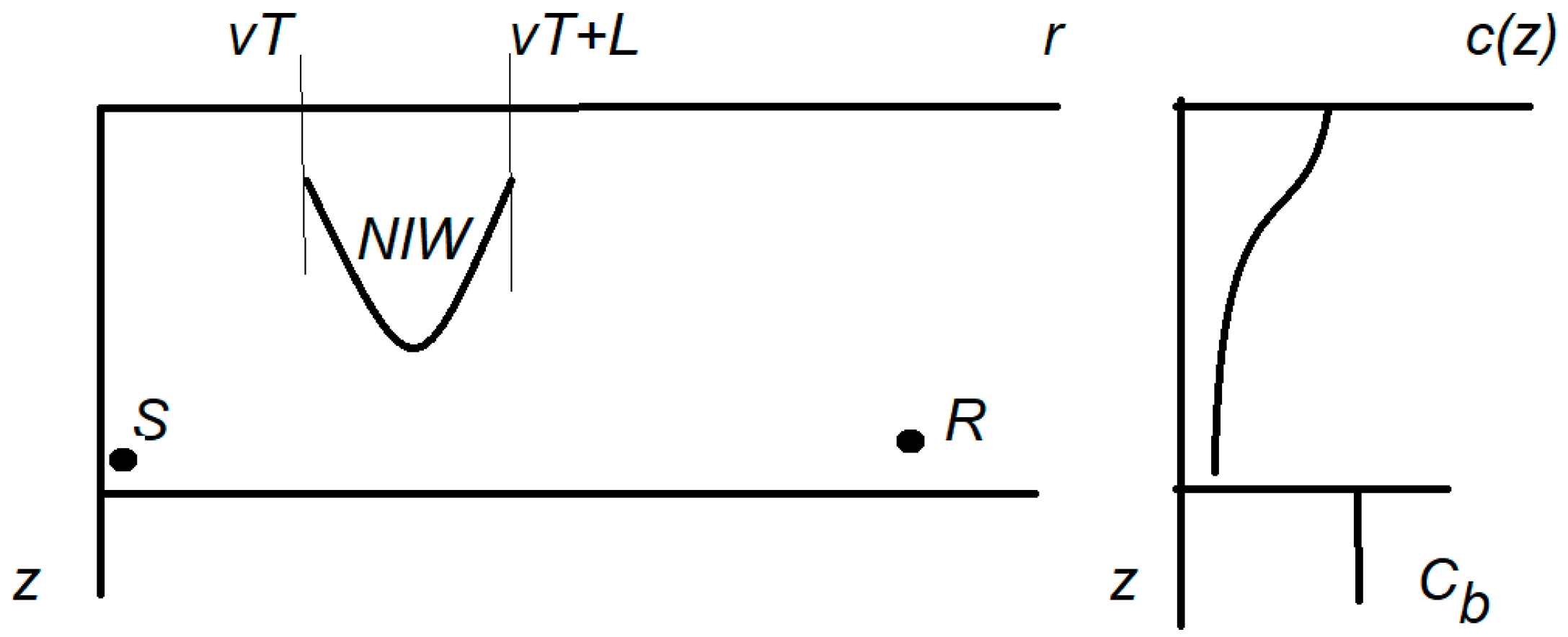
Let’s consider the situation shown in the Figure 1. A localized nonlinear internal wave with horizontal length L moves with speed v in a shallow water waveguide between source and receiver; for simplicity we consider the two-dimensional problem. The depth of the ocean is H, the unperturbed sound speed profile in water is $c_0\left(z\right)$, and the density 𝜌; the bottom is supposed to be liquid homogeneous half-space with sound speed 𝑐_𝑏, and density 𝜌_𝑏.

Let’s find the sound field received by R using a frozen-time approximation, where at any moment of “global” (or slow) time T the medium is stationary. Let’s have a point, the omni-directional source S at the location ($r=0, z=z_0$), emitting a signal with frequency $\omega =2\pi f$ and amplitude $P_0$. The presence of NIWs on acoustic track changes sound speed profile in area of NIWs, and the sound field can be found within the framework of standard perturbation theory [8].

Neglecting horizontal refraction, the complex amplitude of the received signal $P\left(r,z,T\right)$ at an arbitrary point satisfies this equation with the corresponding boundary conditions:

$$\left[\frac{1}{r}\frac{\partial }{\partial r}\left(r\frac{\partial }{\partial r}\right)+\frac{{\partial }^2}{\partial z^2}+k^2\left(z,r,T\right)\right]P=0,$$

(1)

$${P|}_{z=0}=0, {P|}_{z=H-}={P|}_{z=H+}, \frac{1}{\rho }{\frac{\partial P}{\partial z}|}_{z=H-}=\frac{1}{{\rho }_b}{\frac{\partial P}{\partial z}|}_{z=H+},$$

$$k^2\left(z,r,T\right)=k_0^2\left(z\right)+\delta k^2\left(z,r,T\right), k_b=\frac{\omega }{c_b}+i\beta ,$$

Here $\delta k^2\left(z,r,T\right)$ is perturbation of wave number in the water layer due to moving NIWs, β is attenuation coefficient in the bottom.

Let’s consider the modified sound field $\Psi$, excluding cylindrical spreading:

$$P=\frac{\Psi }{\sqrt{r}} .$$

(2)

Within the framework of a mode approach, 𝛹 is sum of waveguide modes with changing amplitudes $C_m\left(r\right)$, as a result of mode coupling (MC) due to local water perturbations $\delta k^2\left(z,r,T\right)$:

$$\Psi \left(r,z\right)={{\displaystyle \sum }}_m^M{C}_m\left(r\right){\psi }_m\left(z\right)\exp \left(i{q}_{m}r\right) .$$

(3)

Here unperturbed eigenfunctions (modes) ${\psi }_m\left(z\right)$ are solutions of the corresponding eigenvalue problem:

$$\left[\frac{d^2}{d{z}^2}+k_0^2\left(z\right)-{\xi }_m^2\right]{\psi }_m\left(z\right)=0,$$

(4)

$${\psi }_m\left(0\right)=0, {\psi }_m\left(H\right)+g_m{\frac{d{\psi }_m}{dz}|}_{z=H}=0 ,$$

$${{\displaystyle \int }}_0^H{\psi }_m^2\left(z\right)dz+\frac{g_m{\psi }_m^2\left(H\right)}{2m_b^2}=1,$$

where ${\xi }_m=q_m+i{\gamma }_m/2$ are complex eigenvalues, properties of the bottom are described by parameter $g_m=i{m}_b/\sqrt{k_b^2-{\xi }_m^2}$, $m_b={\rho }_b/\rho$, M is number of modes, $C_m\left(r\right)$ are modal amplitudes at $r$ = 0: they depend on the depth of the source and have the form: $C_m^0=P_0{(8\pi )}^{-\frac{1}{2}}\exp \left(\frac{i\pi }{4}\right){\psi }_m\left(z_0\right)$. The system of linear equations for $C_m\left(r\right)$ can be derived in a standard way [11]:

$$\frac{d{C}_n}{dr}=-{{\displaystyle \sum }}_1^M{V}_{nm}\left(r,T\right)C_m\exp \left(i\Delta q_{mn}r\right),$$

(5)

$$V_{nm}\left(r,T\right)=\frac{1}{2\sqrt{q_n{q}_m}}{{\displaystyle \int }}_0^H\frac{\rho }{\rho \left(z\right)}{\psi }_n\delta k^2\left(r,z,T\right){\psi }_{m}dz,$$

(6)

$$\mathsf{\Delta }{q}_{mn}=q_m-q_n.$$

Using Figure 1 the area for the solution of (1–6) can be split into three parts: $\left(0<r<vT\right), \left(vT<r<vT+L\right), (vT+L<r)$.

In the first interval modal amplitudes are constant with changing phase, and at the point 𝑟 = 𝑣𝑇 we have: $C_m\left(r=vT\right)=C_m^0\exp \left(i{q}_{m}vT\right)~{\psi }_m\left(z_0\right)\exp \left(i{q}_{m}vT\right)$. We omit the constant factor in the last expression (taking into account bottom attenuation gives a trivial decrease of amplitude with the distance ~${\mathrm{e}}^{-{\gamma }_{m}r/2}$ independently for each mode).

In the second area there is mode coupling and the modal amplitudes change. In the general form

$$C_m\left(r=vT+L\right)={{\displaystyle \sum }}_n^M{S}_{mn}{C}_n^0\exp \left(i{q}_{n}vT\right) ,$$

(7)

where matrix elements 𝑆_𝑚𝑛 depend on properties of waveguides and parameters of NIWs. In the third area modal amplitudes are constant (or decrease due to bottom attenuation) and after the corresponding phase shift we have a sound field at the receiver:

$$\begin{gathered} \Psi \left(r>vT+L,z,T\right)={{\displaystyle \sum }}_m^M{C}_m\left(vT+L\right){\psi }_m\left(z\right){\mathrm{e}}^{i{q}_m\left(r-vT-L\right)}= \\ {{\displaystyle \sum }}_m^M{\psi }_m\left(z\right){\mathrm{e}}^{i{q}_{m}r}{{\displaystyle \sum }}_n^M{S}_{mn}{C}_n^0{\mathrm{e}}^{i(q_n-q_m)vT}={{\displaystyle \sum }}_{n, m}^M{W}_{mn}{\mathrm{e}}^{i(q_n-q_m)vT} , \end{gathered}$$

(8)

where $W_{mn}$ are time T independent values. Thus, we can see that the sound field as a function of T is a quasi-periodical function, containing harmonics at the frequencies

$$F_{mn}=\left|\mathsf{\Delta }{q}_{mn}\right|v/2\pi ,$$

(9)

where the value $\left|\mathsf{\Delta }{q}_{mn}\right|$ is concerned with the spatial scale of interference beating ${\Lambda }_{mn}=2\pi /\left|\mathsf{\Delta }{q}_{mn}\right|$.

The amplitude of spectral component 𝑊_𝑚𝑛 depends on the parameters of a waveguide and NIW. It is clear that a larger amplitude of harmonics corresponds to more strongly interacting modes m and n. Peak frequencies $F_{mn}$ depend on the speed of NIWs and, for typical parameters of shallow water channel and values of speed, peak frequencies are of the order ~2–10 cph. Properties of intensity fluctuations were also considered in ray approximation which can be used for mid and high frequency signals [12,13]. In paper [12], experimental observations of fluctuations with signals ~2–4.5 kHz confirmed the existence of the corresponding peaks. As for the inverse problem, spectra of the sound field fluctuations in the presence of approaching NIWs can give information about their parameters and about the properties of the bottom [14].

3. Modeling of the Sound Fluctuations in the Presence of a Moving Soliton

In this section we present the results of modeling of the sound intensity fluctuations in an underwater sound channel in the presence of NIWs within the framework of a simplified model of the waveguide: the depth H = 50 m, and two layered sound speed profiles:

$$c_0\left(z\right)=\{\begin{array}{c}1520 \mathrm{m}/\mathrm{s}, \mathrm{if} 0<z<20 \mathrm{m},\\ 1470 \mathrm{m}/\mathrm{s}, \mathrm{if} 20 \mathrm{m}<z<50 \mathrm{m}\end{array}$$

(10)

𝑐_𝑏 = 1700 m/s in the bottom, $m_b=$ 1.7, the attenuation coefficient is $\beta$= 0.4 dB/$\lambda$.

The length of the acoustic track is 14 km, and the model of NIWs is a KdV soliton with amplitude 10 m and wavelength 300 m. It is moving from the source to receiver with a speed of 1 m/s.

Calculation of the sound field at frequency 500 Hz for each position of moving NIWs, or for each moment of time T, was carried out using a two-dimensional parabolic equation for the function $\Psi \left(r,z,T\right)$ with the following decomposition using orthogonality of waveguide modes. Modal amplitudes are:

$$C_m\left(r, T\right)={\displaystyle \int }\frac{\rho }{\rho \left(z\right)}\Psi \left(r,z,T\right){\psi }_m\left(z\right)dz.$$

(11)

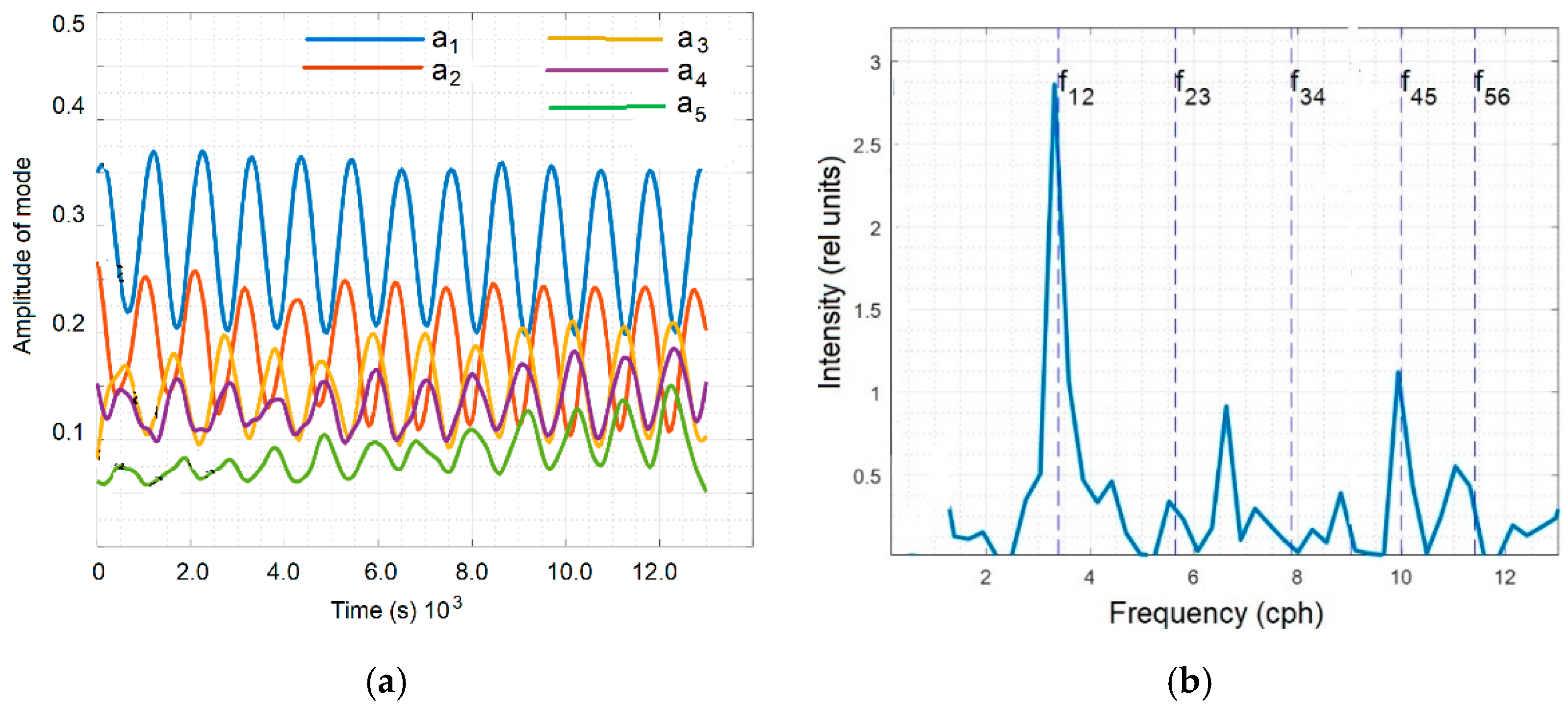
In Figure 2a, modal amplitudes at the receiver are shown for the lowest 5 modes as a function of the “global” time T, where T is taken every 60 s. Predominant periods of oscillation are seen, and we can see also the comparatively small contribution of more high frequencies. The calculated spectrum $S\left(\mathsf{\Omega }\right)$ of sound intensity is shown in Figure 2b

$$S\left(\mathsf{\Omega }\right)={\displaystyle \int }{\left|\Psi \right|}^2{e}^{-i\mathsf{\Omega }T}dT ,$$

(12)

the biggest peak (predominating frequency $\mathsf{\Omega }$ ~ 3 cph) corresponds to the most significant coupling of modes 1 and 2.

Thus, if we hypothesize an experimental situation where the sound field is being measured at the receiver during the rather long time of soliton’s passing (about a few hours, in our example 4 h), then the analysis of the spectrum of fluctuations, like in Figure 2b, allows us to estimate speed of NIWs and, possibly, its amplitude if waveguide parameters are known and do not change along the acoustic track. At the same time, it is clear that if the parameters of waveguide (for example depth and/or sound speed profile) change along acoustic track, and, as a result, the parameters of the NIW change also, then positions of peaks in spectrum and their amplitudes change with time T as well, and in particular, a solution of the inverse problem in a given statement is impossible or needs a more detailed analysis.

In the next sections a similar situation will be studied using the data of experiment ASIAEX 2001, where there are significant variations of bathymetry.

4. Experiment ASIAEX 2001

In this section, we consider the sound fluctuations during the motion of an NIW between source and receiver in a waveguide with significantly variable depth $H\left(r\right)$ and, correspondingly, variable speed $v\left(r\right)$. In this case the dominant frequencies of the sound intensity fluctuations are determined by (9) with local parameters at the current position of the soliton, or by the current time $T$: $F_{mn}\left(T\right)=v\left(T\right)/{\Lambda }_{mn}\left(T\right)$ where $v\left(T\right)$ is the soliton’s velocity and ${\Lambda }_{mn}\left(T\right)$ is the length of spatial interference beating. It is shown below, that the experiment and simulation give an interesting result of the approximate constancy of the dominant frequency: $F_{mn}\left(T\right)~$ const.

The analysis is carried out for one of the episodes (7 May 2001, 04:00–14:00) of the ASIAEX 2001 experiment in the South China Sea [1]. The main purpose of this experiment was to study the propagation of sound signals under conditions of significant water instability in the area of the shelf break, manifested in the generation of large-amplitude soliton-like NIWs.

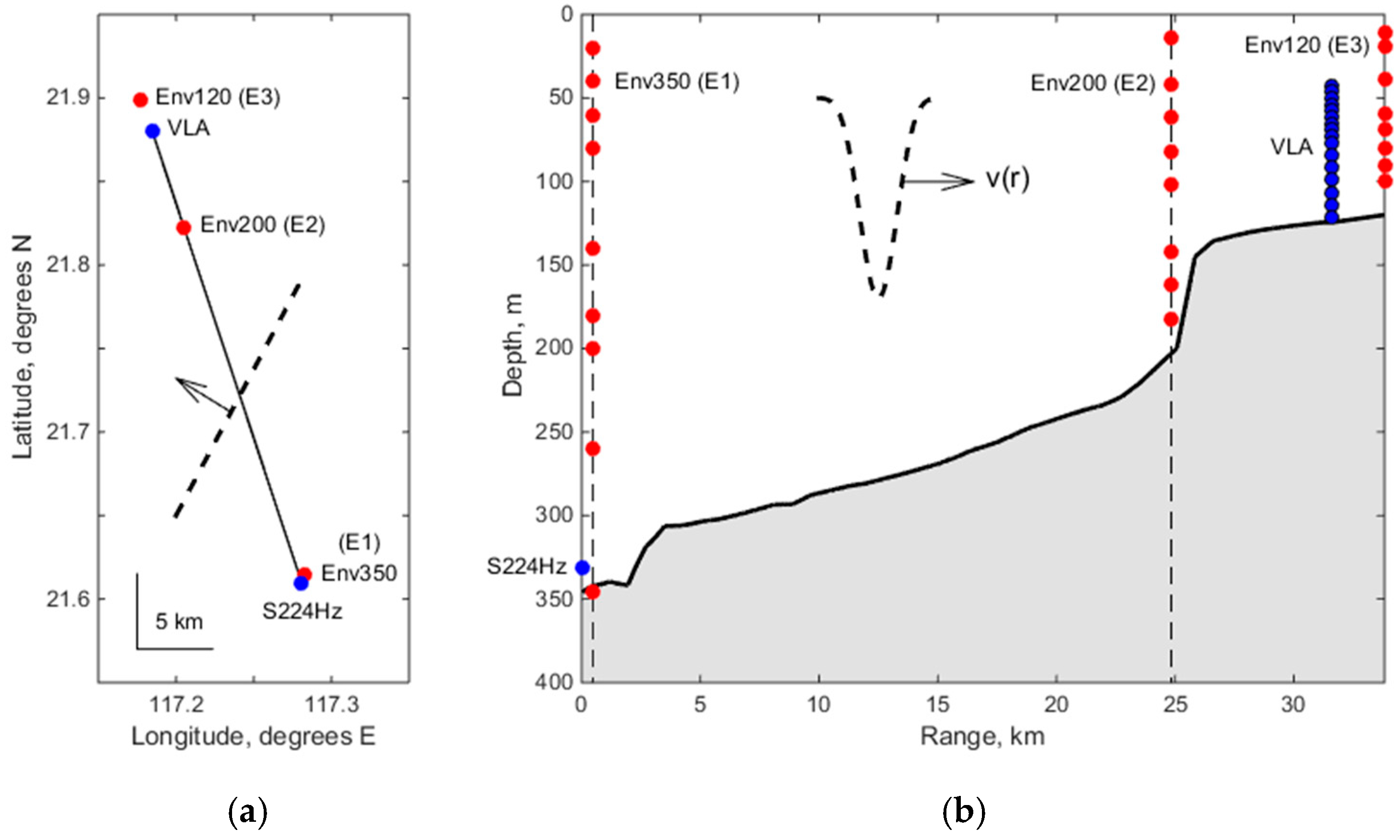
The acoustic track, which is considered below, was ~32 km long (Figure 3). It was oriented perpendicular to the coastal line and consisted of two intervals: (1) a relatively deep-water part with a smooth depth variation: from 350 to 200 m at a distance of 25 km; (2) a shallow-water part with a depth of 120 m, starting after a steep slope of the bottom. In this region, during the entire time of the experiment (April–August 2001), NIWs in the form of single solitons of an amplitude up to 100 m were observed about twice a day. NIWs were registered in different ways: using satellite images of characteristic roughness on the water surface, using records of thermistor chains and Acoustical Doppler Current Profiler. 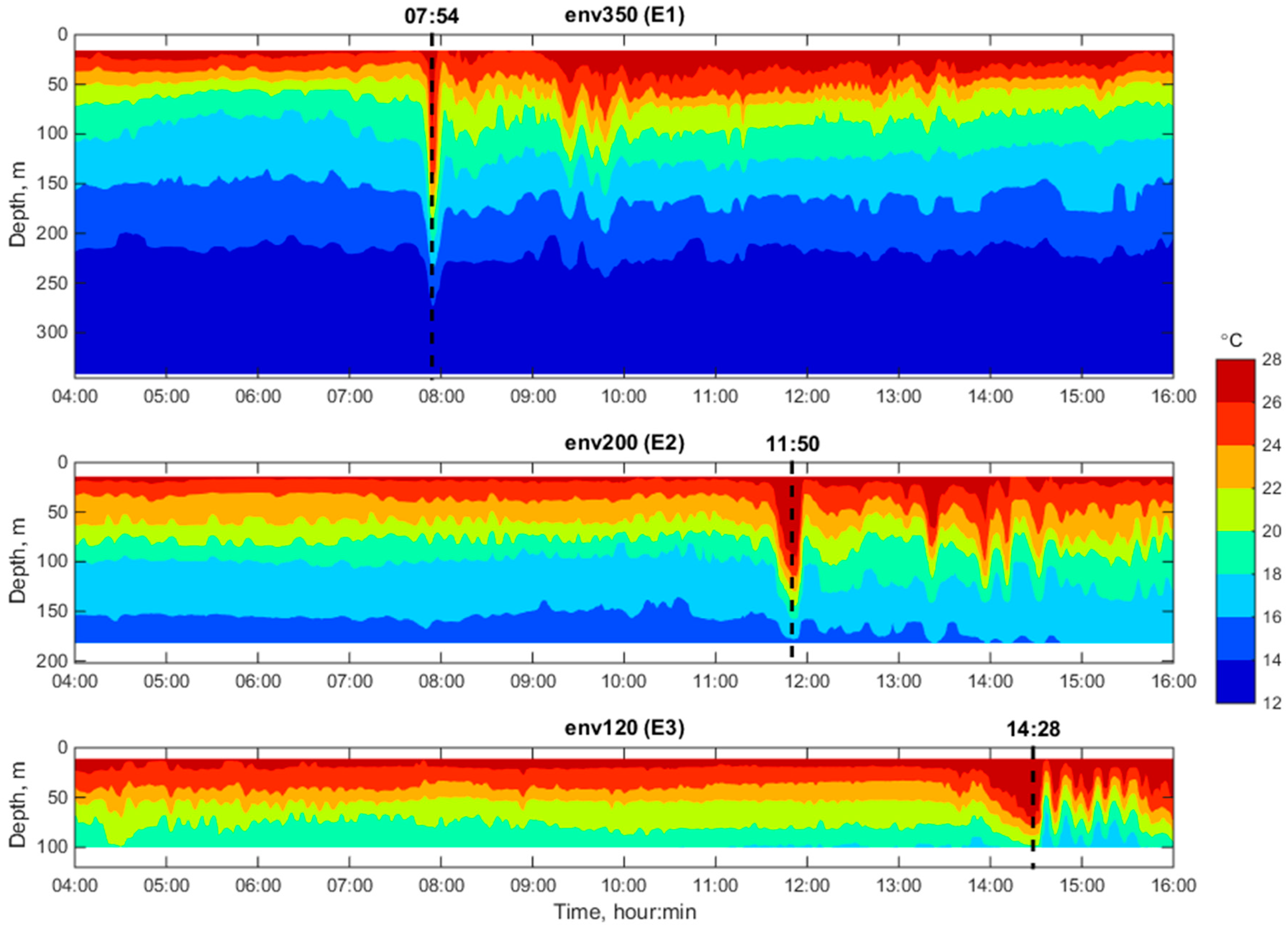In our case, according to satellite observations [4], the soliton moved approximately at an angle of 45° to the acoustic track indicated by the arrow in Figure 3. Temperature records are shown in Figure 4.

Three vertical thermistor chains Env350, Env200 and Env120 (abbreviated as E1, E2, E3) were deployed along the acoustic track which consisted of 9 (E1) and 8 (E2, E3) thermistors. The chains were installed close to the S224Hz source at the shelf break, and in the vicinity of the receiving antenna (VLA), correspondingly (Figure 3). In this case, as can be seen from Figure 3a, the objects S224Hz, E2, VLA and E3 are located along the same line (the corresponding distances are given in

Table 1. Basic parameters of the experiment (13:42 *—calculated value).

	Depth of the Sea (m)	Distance to the Source	Arrival Time of Soliton (h:min)
S224Hz	345.8	–	T1 = 07:54
env200 (E2)	202	R2 = 24,838 m	T2= 11:50
VLA	124.5	R = 31,597 m	TR = 13:42 *
env120 (E3)	120	R3 = 33,820 m	T3= 14:28

). The E1-chain is located away from this line, at a distance of 591 m from the S224Hz source. However, the orientation of E1 with respect to S224Hz was chosen so that when the front of the soliton moves (dashed line in Figure 3a), the times of its arrival at S224Hz and E1 practically coincide (the mismatch is less than one period of emission of S224Hz pulses, equal to 5 min, which, when analyzing sound fluctuations, will be equal to the sampling interval of the vertical of the source). For this reason, we suppose that the thermistor chain E1 gives the depth distribution of temperature at the source’s location.

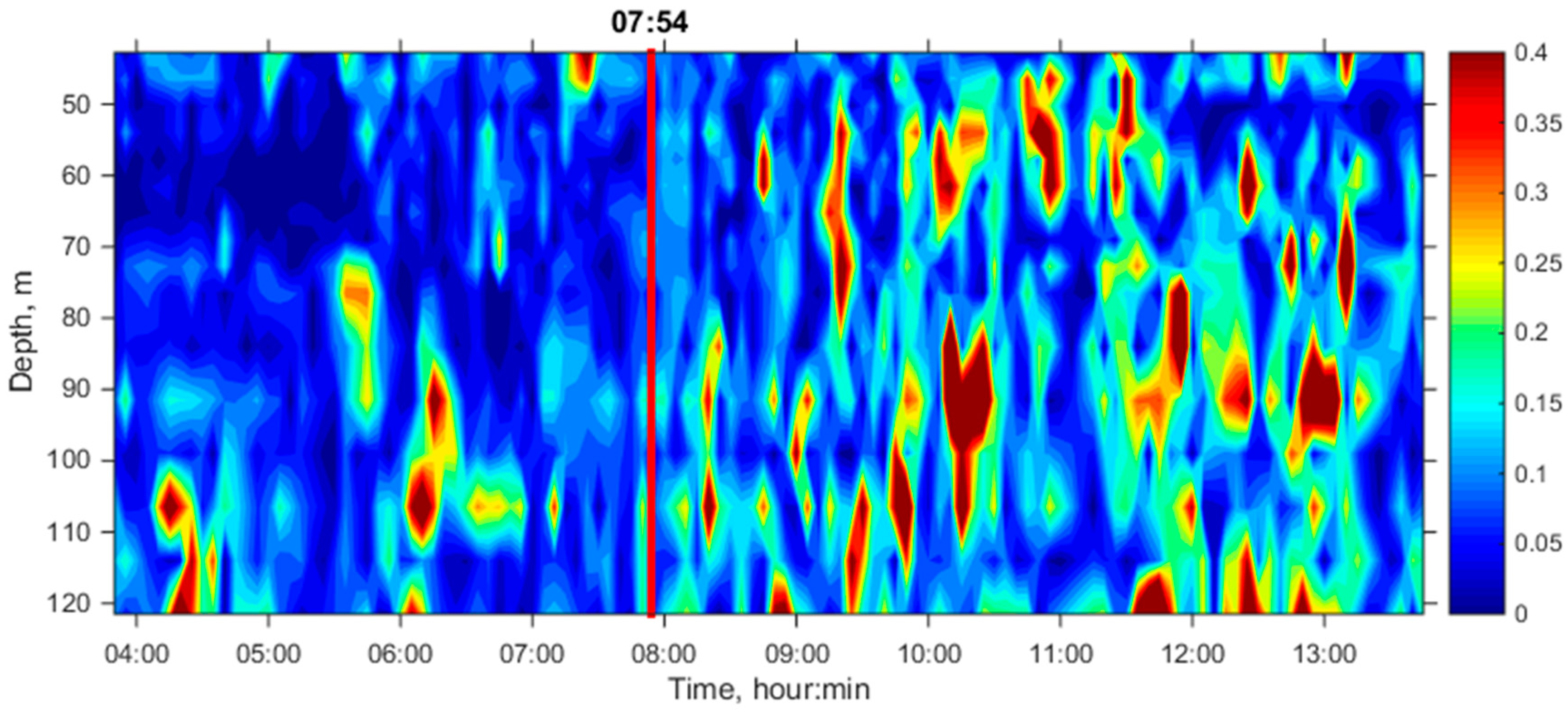
Figure 4 shows records of the thermistor strings E1, E2, and E3 during 4:00–16:00 on 7 May 2001. A 100-m soliton is clearly visible, arriving at the chains after a relative calm. The arrival times of this soliton on the chains are, respectively:$T_1=$ 07:54, $T_2=$ 11:50, $T_3=$ 14:28. Knowing the distances between the chains (Table 1), we find that the average soliton velocity in the deep-water part E1–E2 is $v_{12}=\frac{R_2}{T_2-T_1}=1.75$ m/s and in the shallow-water part E2–E3, $v_{23}=\frac{R_3-R_2}{T_3-T_2}=$ 0.95 m/s. Thus, we have the motion of a soliton with variable speed.

Let us further find the velocity of a soliton as a function of distance $v\left(r\right)$, where r is the distance from the source to the soliton along the acoustic track (Figure 3b). To do this, we use the depth dependence of the soliton’s velocity, obtained within the framework of the water model with two layers of different densities [15]:

$$v\left(r\right)=\sqrt{\frac{g^{\prime }{h}_1\left(H\left(r\right)-h_1\right)}{H\left(r\right)}} ,$$

(13)

where $h_1$ is the thickness of the upper layer, $g^{\prime }={\cos }^{-2}\alpha ·g\Delta \rho /\rho$ is the reduced gravitational acceleration, α is the angle between the velocity vector of the soliton’s front and the direction of the source-receiver path (in our case, ~45°), $g=$ 10 m/s², $\Delta \rho /\rho$ is the relative difference in the density of the layers. Note that, in contrast to [15], a factor ${\cos }^{-2}\alpha$ is introduced into the coefficient, since we are interested in the velocity of the soliton along the acoustic track.

Let us apply this model to our case, considering $h_1$ also $g^{\prime }$ as the fitting coefficients to be determined. The determination of the coefficients will be based on minimizing the mismatch

$$\sigma \left(h_1,g^{\prime }\right)=\sqrt{{\left(T_{12}-T_{12}^{\prime }\right)}^2-{\left(T_{23}-T_{23}^{\prime }\right)}^2} ,$$

(14)

where $T_{12}=T_2-T_1$ and $T_{23}=T_3-T_2$ are the difference in arrival times measured in the experiment; $T_{12}^{\prime }={{\displaystyle \int }}_0^{R_2}\frac{dr}{v\left(r\right)}$ and $T_{23}^{\prime }={{\displaystyle \int }}_{R_2}^{R_3}\frac{dr}{v\left(r\right)}$ are similar times calculated according to (13) for given $h_1$ and $g^{\prime }$.

Calculations give the minimum mismatch at $h_1$= 106.27 m, $g^{\prime }$= 0.04773 m/s². Figure 5 shows the resulting function.

Let us now consider the sound speed profiles for simulating the sound propagation in a waveguide constructed using the temperature profiles (Figure 4). Figure 6a shows the unperturbed temperature profile measured at a certain time using a shipborne CTD probe near the source (CTD 2 in [1]). Using the complete CTD data (conductivity, temperature, depth data), the corresponding sound speed profile (SSP) was calculated (Figure 6b). It can be seen that the SSP approximately repeats the temperature profile. This means that one temperature is sufficient to determine the SSP. Figure 6c shows the temperature dependence of the speed of sound. The fitted polynomial of the second degree gives the formula for converting the temperature into the speed of sound in the given region of the experiment:

$$c=-0.0313{\tau }^2+3.66\tau +1461.5 \mathrm{m}/\mathrm{s}$$

(15)

where $\tau$ is the temperature in degrees Celsius.

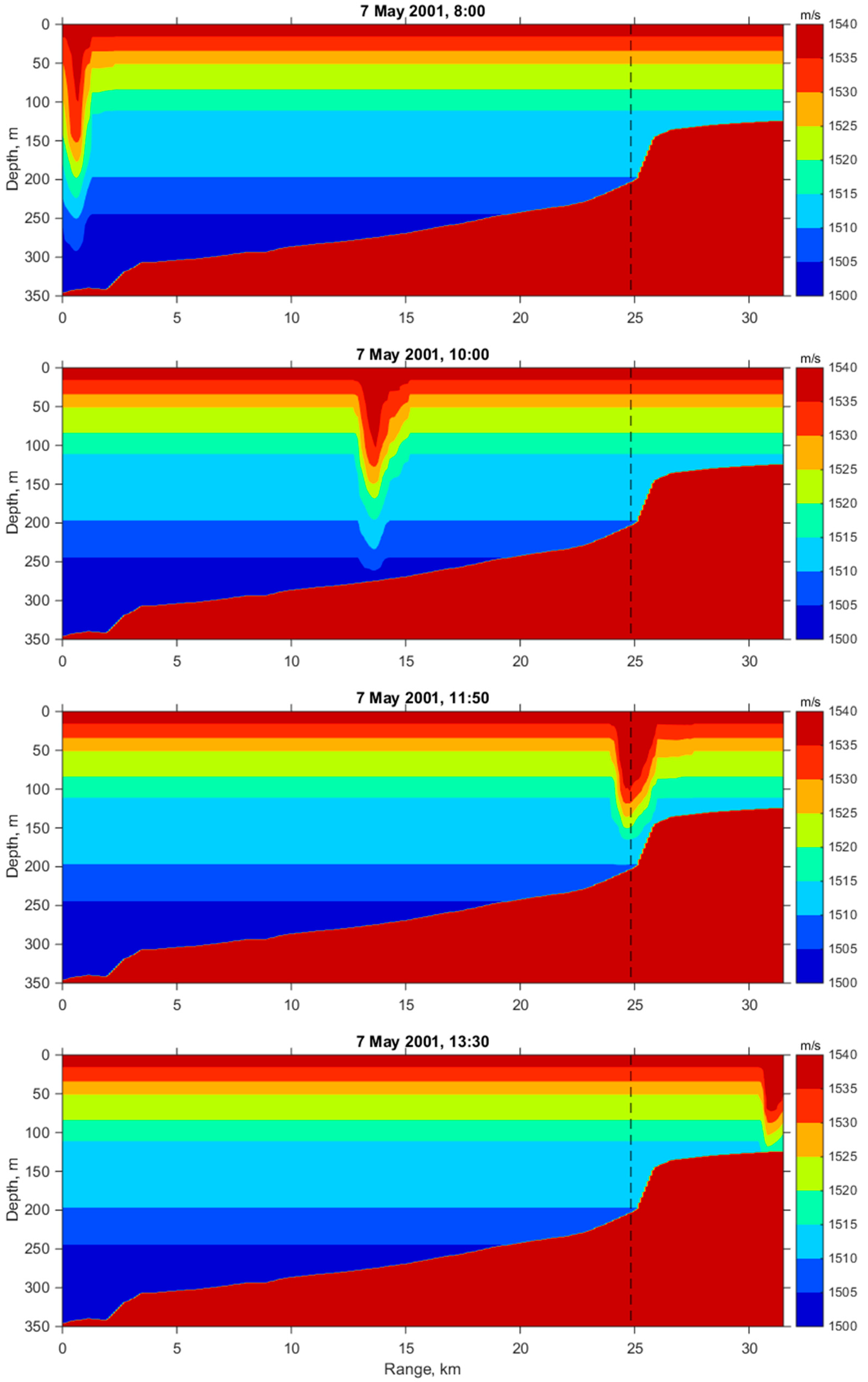
The final stage in the consideration of the oceanographic situation is the modeling of the sound speed field in the channel, i.e., obtaining the function $c\left(r,z,T\right)$ during the time of passage of the soliton along the path using the data of thermistor chains (Figure 4) and the calculated velocity of the soliton (Figure 5).

Let $c\left(0,z,T\right), c\left(R_2,z,T\right), c\left(R_3,z,T\right)$ be sound speed profiles on the thermistor chains E1, E2, E3, obtained using (15) from temperature profiles (Figure 4). Using these data, reconstruction of the sound speed $c\left(r,z,T\right)$ for the acoustic track $0\le r\le R$ from the source to receiver can be done from:

$$\begin{gathered} c\left(r,z,T\right)=c\left(0,z,T-T_{1r}\right)\frac{R_2-r}{R_2}+c\left(R_2,z,T+T_{r2}\right)\frac{r}{R_2}, 0<r\le R_2 , \\ c\left(r,z,T\right)=c\left(R_2,z,T-T_{2r}\right)\frac{R_3-r}{R_3-R_2}+c\left(R_3,z,T+T_{r3}\right)\frac{r-R_2}{R_3-R_2}, R_2<r\le R \end{gathered}$$

(16)

where $T_{1r}^{}={{\displaystyle \int }}_0^r\frac{dr}{v\left(r\right)}$, $T_{r2}^{}={{\displaystyle \int }}_0^{R_2}\frac{dr}{v\left(r\right)}$, $T_{2r}={{\displaystyle \int }}_{R_2}^r\frac{dr}{v\left(r\right)}$, $T_{r3}^{}={{\displaystyle \int }}_r^{R_3}\frac{dr}{v\left(r\right)}$.

We remark that for constant speeds $v_{12}$ and $v_{23}$ of the soliton on the first and second parts of the acoustic track we obtain more simple expressions [16]:

$$\begin{gathered} c\left(r,z,T\right)=c\left(0,z,T-\frac{r}{v_{12}}\right)\frac{R_2-r}{R_2}+c\left(R_2,z,T+\frac{R_2-r}{v_{12}}\right)\frac{r}{R_2}, 0<r\le R_2 \\ c\left(r,z,T\right)=c\left(R_2,z,T-\frac{r-R_2}{v_{23}}\right)\frac{R_3-r}{R_3-R_2}+c(R_3,z,T+\frac{R_3-r}{v_{23}})\frac{r-R_2}{R_3-R_2}, R_2<r\le R \end{gathered}$$

(17)

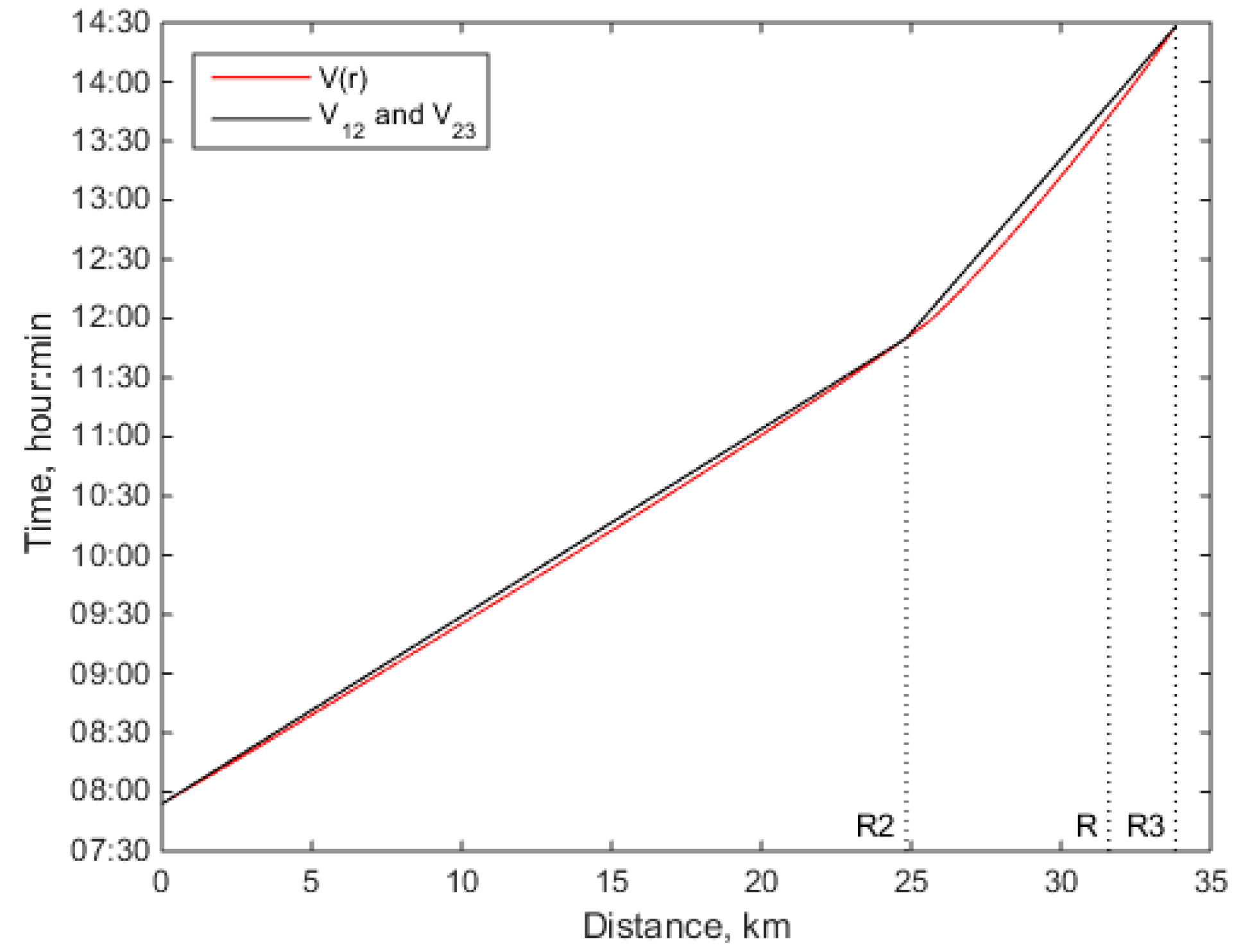
In Figure 7, the reconstruction of the sound speed is shown using (16). Here, only the passage of the soliton is considered.

It turns out that the use of “step-like” reconstruction according to (17) does not significantly change the result. As follows from Figure 8, the arrival time of the soliton to the same points on the path differs insignificantly. The maximum difference is 9.4 min, which is less than two periods of intensity sampling interval $2\Delta T$ when analyzing sound fluctuations (see below). In this case, the calculated arrival time of the soliton at the receiver is 13:42 when $v\left(r\right)$ is used, and 13:48 when using $v_{12}$ and $v_{23}$.

5. Fluctuations of the Sound Intensity in the Experiment

The main characteristics of the source and receiver used in the experiment are here. S224Hz is a pulse source of phase-shift keying signals (M-sequences) emitted at a central frequency of 224 Hz. The duration of one pulse is ~2 min (118.125 s), the repetition period is $\Delta T=$ 5 min. The source depth is $z_0=$ 331.3 m, where sea depth is 345.8 m. The VLA is a vertical receiving antenna consisting of 16 hydrophones. The hydrophones were numbered from the top to the bottom: the depth of the upper hydrophone was $z_1=$ 42.75 m, the depth of the lower one was $z_{16}=$ 121.5 m, the sea depth is 124.5 m. The interval between adjacent hydrophones 1–10 was 3.75 m, the interval between adjacent hydrophones 10–16 was 7.5 m.

Let T be the “slow” time, considered as a parameter and discretized with intervals $\Delta T$. Let t be “quick” time, in the range $0<t\le \Delta T$. In that case, each pressure pulse received at depth z can be written in the form $p\left(t,z,T\right)$. We analyze the pulses at a central frequency of $f=$224 Hz. To do this, we find the complex amplitude of the signal at a given frequency $P\left(z,T\right)=2{{\displaystyle \int }}_0^{\Delta T}p\left(t,z,T\right)\exp \left(i2\pi ft\right)dt$ and calculate the intensity

$$I\left(z,T\right)={\left(2\rho \overline{c}\right)}^{-1}{\left|P\left(z,T\right)\right|}^2$$

(18)

where $\rho =$ 1 g/cm³ is the density of water, $\overline{c}=$1500 m/s is the average speed of sound in water.

Let’s consider 120 received pulses corresponding to the 10-h observation interval 03:50–13:45. During the first 4 h (03:50–07:54), the soliton is off the acoustic track. During the next 6 h (07:54–13:42) the soliton moves from the source to the receiver. Ideally, the intensity should be constant in the absence of a soliton on the acoustic track and fluctuations should be observed in the presence of a soliton. In reality, due to background internal waves, ambient noise, etc., fluctuations are always observed, but it can be assumed that, in the presence of a soliton, the amplitude of fluctuations increases.

To confirm this assumption, we divide the observation interval into 5 sections of D = 2 h each. Then, for each section with central time $T_0$, we find the average intensity $\overline{I}\left(z,T_0\right)=D^{-1}{{\displaystyle \int }}_{T_0-0.5D}^{T_0+0.5D}I\left(z,T\right)dT$ and the modulus of the variable component $\left|\tilde{I}\left(z,T,T_0\right)\right|=\left|I\left(z,T\right)-\overline{I}\left(z,T_0\right)\right|$. Figure 9 shows the resulting dependence $\left|\tilde{I}\left(z,T,T_0\right)\right|$ for all five values $T_0$. It can be seen that after the arrival of the soliton on the path (07:54), the amplitude of fluctuations became noticeably higher (the standard deviation was in average 2.5 times larger), and significant fluctuations were observed at all hydrophones of the VLA.

Let us consider further the spectrogram of intensity fluctuations in the form:

$$G\left(\mathsf{\Omega }, T\right)={{\displaystyle \sum }}_{j=1}^J\left|{{\displaystyle \int }}_{T_0-0.5D}^{T_0+0.5D}\tilde{I}\left(z_j,T^{\prime },T\right)w\left(T^{\prime }\right)\exp \left(i\mathsf{\Omega }{T}^{\prime }\right)d{T}^{\prime }\right|$$

(19)

where $z_j$ are the depths of hydrophones, J = 16 is the total number of hydrophones, D = 1.5 h is the value of the sliding Fourier window, $w\left(T^{\prime }\right)$ is the window function, $\mathsf{\Omega }=2\pi F$ is the angular frequency of fluctuations, $\tilde{I}\left(z_j,T^{\prime },T\right)=I\left(z_j,T^{\prime }\right)-D^{-1}{{\displaystyle \int }}_{T_0-0.5D}^{T_0+0.5D}\tilde{I}\left(z_j,T^{\prime }\right)d{T}^{\prime }$ is the variable component of the intensity in the window $D$ as a function of the current time $T^{\prime }$, at the position of the center of the window equal to $T$.

Figure 10 shows the spectrogram (19) obtained using a gate window, i.e., if $w\left(T^{\prime }\right)$ = 1. In Figure 10a, the picture is normalized to the global maximum; in Figure 10b, to the local maximum at each vertical. In Figure 10a, as in Figure 9, it is clearly seen that the amplitude of fluctuations increases as a whole, noticeably after the arrival of the soliton on the path. In addition, an increase of the fluctuations’ amplitudes is observed when the soliton passes the shelf break (around 11:50). Figure 10b clearly shows the dominant fluctuation frequency (red bar). It is approximately at the same level of $F_D$ ~ 1 cph for the entire observation period.

Let’s clarify the value of the dominant frequency. To do this, we find a spectrogram using the Hamming window. The result is shown in Figure 11. Here, the picture is normalized to a local maximum for each time. In addition, for convenience, a different color gradation is used. In contrast to Figure 10b, the dominant frequency in Figure 11 looks like a continuous yellow bar on which the maximal value on the spectrogram is shown by a thin black line.

The average value of the dominant frequency in the absence of a soliton on the path (before 07:54) is $F_D=$0.92 ± 0.04 cph, and in the presence of a soliton (after 07:54) it is $F_D$= 1.4 ± 0.1 cph. The presented mean values and their confidence intervals (with a confidence level of 95%) are shown in Figure 11 by horizontal lines.

The difference in the dominant frequencies is probably due to the fact that the adiabatic mechanism of fluctuations predominates in the first time interval. Here, the intensity fluctuations are determined mainly by the Brunt–Väisälä frequency; oscillations of water at the source and receiver due to background internal waves, in the absence of mode coupling. In the second time interval, the mechanism of mode coupling on a moving soliton prevails. The frequency of these fluctuations is close to the Brunt–Väisälä frequency, as noted, in particular in [9], but in the general case it is not equal. Indeed, the dominant frequency of sound fluctuations due to mode coupling depends on the velocity of the soliton along the acoustic track. The speed of a soliton is, in a sense, an arbitrary value, since it depends on the mutual orientation of the soliton front and the direction of acoustic track.

6. Modeling Fluctuations

Let us consider further the time interval 07:54–13:42 only, when the soliton passes completely through the distance from the source to the receiver. The problem of modeling the sound intensity fluctuations is based on the oceanographic data described above.

Let’s solve the problem in the frozen time approximation, where we solve the stationary wave equation at each moment of the time T. Let a point isotropic source be at the point $z=z_0, r=0$ and emit a signal of complex amplitude $P_0$ with a sound frequency $\omega =2\pi f$. The modeling of the sound field is carried out within the framework of theory of mode coupling, taking into account both moving NIW and changing bathymetry as additional dependence of waveguide parameters on r. Neglecting horizontal refraction, the complex amplitude of the received signal $P\left(r,z\right)$ an arbitrary point $\left(r,z\right)$ can be found from the solution of the Helmholtz equation with the corresponding boundary conditions and radiation conditions at infinity

$$\left\{\frac{1}{r}\frac{\partial }{\partial r}\left(r\frac{\partial }{\partial r}\right)+\frac{{\partial }^2}{\partial z^2}+K^2\right\}P=-P_0\delta \left(z-z_0\right)\frac{\delta \left(r\right)}{2\pi r}$$

(20)

$${P|}_{z=0}=0, {P|}_{z=H-}={P|}_{z=H+}, \frac{1}{\rho }{\frac{\partial P}{\partial z}|}_{z=H-}=\frac{1}{{\rho }_b}{\frac{\partial P}{\partial z}|}_{z=H+}$$

where $K=\{\begin{array}{c}k, 0<z<H\\ k_b, z>H\end{array}, H=H\left(r\right), k=\frac{\omega }{c\left(r,z,T\right)}$, $k_b=\frac{\omega }{c_b}+i\beta$, $\delta (.)$ is Dirac delta function, $\partial /\partial n$ derivative over normal to the bottom-water interface. The parameter $P_0$ characterizing the power and the initial phase of the source does not play a role in the following since it disappears upon normalization. We take the bottom parameters from [16]: the sound speed $c_b$ is 1600 m/s, the density ${\rho }_b$ is 1.6 g/cm³ and the attenuation $\beta$ is 0.8 dB/λ.

We assume that variations of the waveguide’s parameters are smooth in the horizontal plane so $\partial /\partial n\approx \partial /\partial z$. Then, we take into account mode coupling due to perturbation in the water layer and variation of bathymetry; so a solution to (20) in the water layer $(0<z<H)$ has the form of decomposition over adiabatic waveguide modes:

$$P={{\displaystyle \sum }}_{m=1}^M{C}_m\left(r\right)\frac{{\psi }_m\left(r,z\right)}{\sqrt{q_m\left(r\right)r}}\mathrm{e}\mathrm{x}\mathrm{p}\left(i{{\displaystyle \int }}_0^r{q}_m\left(r^{\prime }\right)d{r}^{\prime }\right)$$

(21)

$$\left[\frac{d^2}{d{z}^2}+k^2\left(z\right)-{\xi }_m^2\right]{\psi }_m\left(z\right)=0,$$

(22)

$${\psi }_m\left(0\right)=0, {\psi }_m\left(H\right)+g_m{\frac{d{\psi }_m}{dz}|}_{z=H}=0 ,$$

$${{\displaystyle \int }}_0^H{\psi }_m^2\left(z\right)dz+\frac{g_m{\psi }_m^2\left(H\right)}{2m_b^2}=1,$$

where ${\psi }_m$ and ${\xi }_m=q_m+i{\gamma }_m/2$ are adiabatic (local) eigenfunctions and eigenvalues of the Sturm problem (22), depending on r as on parameter; $m_b={\rho }_b/\rho$, $g_m=i{m}_b/\sqrt{k_b^2-{\xi }_b^2}$, M is number of modes taken into account, $C_m$ are modal amplitudes, which at $r=0$ have the form $C_m\left(0\right)=P_0{\left(8\pi \right)}^{-1/2}\exp \left(\frac{i\pi }{4}\right){\psi }_m\left(0,z_0\right)$, for other r they can be found from the system of linear equations:

$${{\displaystyle \sum }}_{n=1}^M\left[\left({\delta }_{mn}-I_{mn}\right)E_n\right]\frac{d{C}_n}{dr}={{\displaystyle \sum }}_{n=1}^M{C}_n\left[V_{mn}+\frac{{\gamma }_n}{2}\left({\delta }_{mn}-I_{mn}\right)\right]E_n$$

(23)

$$V_{mn}=\underset{0}{\overset{H}{{\displaystyle \int }}}{\psi }_m\frac{\partial {\psi }_n}{\partial r}dz$$

here $V_{mn}$ are mode coupling coefficients, ${\delta }_{mn}=\{\begin{array}{c}1, m=n\\ 0,m\ne n \end{array}$ is Kroneker delta

$$I_{mn}=\frac{i{\psi }_m\left(H\right){\psi }_n\left(H\right)}{m_b\left({\epsilon }_m+{\epsilon }_n\right)}, E_n=\sqrt{q_n}\exp \left(i{{\displaystyle \int }}_0^r{q}_n\left(r^{\prime }\right)dr\prime \right), {\epsilon }_{m,n}=\sqrt{k_b^2-{\xi }_{m,n}^2} .$$

All of the above radicals $\sqrt{*}$ are understood unambiguously as the principal value of the complex square root, in which $\mathrm{Re}\left\{\sqrt{*} \right\}>0$. If $\mathrm{Re}\left\{\sqrt{*} \right\}=0$, then the value is selected which has $\mathrm{Im}\left\{\sqrt{*} \right\}>0$. This rule corresponds to the sqrt function in MATLAB. With such a rule for determining the radical, the solution (22) gives an infinite number ${\xi }_m$ and ${\psi }_m$, i.e., an infinite number of modes [17]. When calculating the field, it is sufficient to restrict oneself to a finite number of modes for which additional modes do not play a role. Calculations have shown that at a frequency of $f=$ 224 Hz it will be sufficiently limited by the number of modes $M=11$, which corresponds to the total number of propagating modes in the shallow water area near the receiver.

The solution of the linear system (23) at known values of $C_m\left(r\right)$ gives derivatives $C_m^{\prime }=d{C}_m/dr$, which in turn allows calculating the mode coefficients at the next step: $C_m\left(r+\mathsf{\Delta }r\right)=C_m\left(r\right)+C_m^{\prime }\mathsf{\Delta }r$. Thus, knowing $C_m\left(0\right)$, one can find functions $C_m\left(r\right)$ for any $r$.

Note that system (23) is obtained by substituting (21) into the homogeneous Helmholtz equation (20), where the right-hand side is equated to zero (the area outside the source). Then, standard approximations are carried out, in which all terms of higher order of smallness are neglected, and, also, the equation for the eigenfunctions (22) and the condition of orthogonality of the eigenfunctions in the form ${{\displaystyle \int }}_0^H{\psi }_m{\psi }_{n}dz+I_{mn}={\delta }_{mn}$ are used. A detailed conclusion is given in [18].

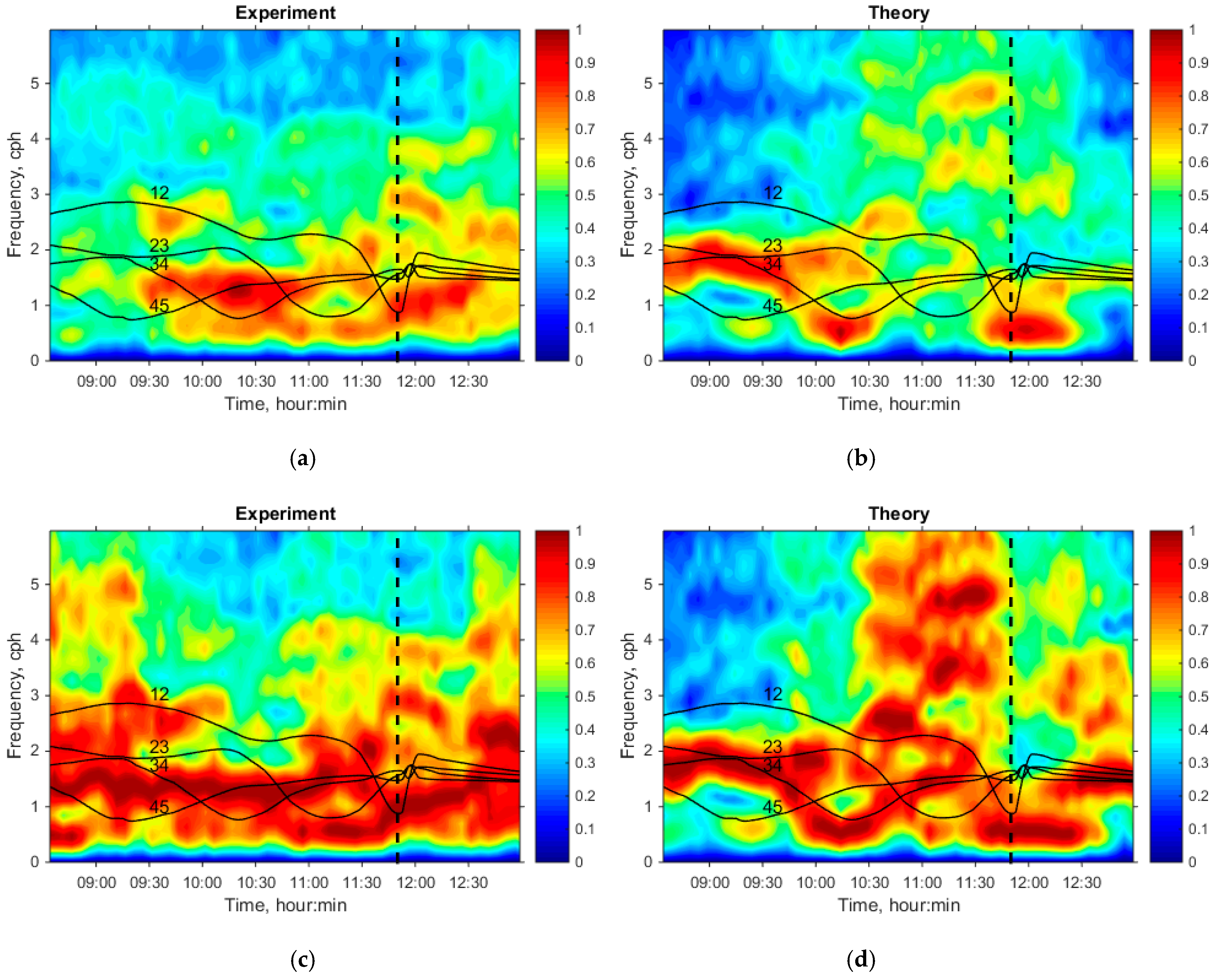
Thus, using (21), we find the theoretical field in the waveguide, more exactly, at the VLA. Further, similar to the processing experiment, we use Formulas (18) and (19) to find the theoretical spectrogram. Figure 12 shows the results of calculations in comparison with the experiment. In this case, a gate window was used to obtain a spectrogram. As one can see, there is good agreement, which is primarily due to a fairly complete description of the oceanographic situation.

Figure 12 also shows the dependencies

$$F_{mn}\left(T\right)=\frac{v\left(T\right)}{{\mathsf{\Lambda }}_{mn}\left(T\right)} ,$$

(24)

where $F_{mn}\left(T\right)$ is the theoretical frequency of intensity fluctuations due to the interacting pair of modes ($m,n$) and observed at the moment of time T; $v\left(T\right)$ and ${\mathsf{\Lambda }}_{mn}\left(T\right)$ are the initial distance functions recalculated as a function of time: $v\left(r\right)$ is the velocity of the soliton and ${\mathsf{\Lambda }}_{mn}\left(r\right)=2\pi {\left|q_m-q_n\right|}^{-1}$ is the spatial interval of interference beating of a pair of modes ($m,n$). The recalculation of the distance in time was carried out according to the formula $T=T_1+{{\displaystyle \int }}_0^r{v}^{-1}\left(r\right)dr$, where $T_1=$ 7:54.

In Figure 12 dependencies $F_{mn}\left(T\right)$ are shown by solid lines for adjacent pairs of modes 12, 23, 34, 45. This is due to the fact that modes 2, 3, 4 dominate in the channel (Figure 13) and the maximum of mode coupling takes place between adjacent modes. As can be seen from Figure 12, the maximum fluctuations indeed correspond to the indicated pairs of modes, which confirms the hypothesis about mode coupling as the reason behind the fluctuations. It can also be seen that the lines $F_{mn}\left(T\right)$ are generally horizontal, which explains the approximate constancy of the dominant frequency. Let’s obtain an estimate for observed dominant frequency as the average between the corresponding curves under consideration during the time interval of the soliton’s motion from the source to the receiver (from $T_1$ to $T_R$):

$$F_D=\frac{1}{4\left(T_R-T_1\right)}{{\displaystyle \sum }}_{m=1}^4{{\displaystyle \int }}_{T_1}^{T_R}{F}_{m, m+1}\left(T\right)dT$$

(25)

Calculations give $F_D=$1.65 cph, that is close to value $F_D=$ 1.4 ± 0.1 cph obtained from the experiment (see the right side of Figure 11).

At the same time, the slightly reduced experimental value of the dominant frequency, in comparison with the theoretical one, can be explained by the presence in the experiment of adiabatic fluctuations at the Brunt–Väisälä frequency (see the left side in Figure 11), the value of which is less than the frequency of fluctuations caused by the mode coupling. When two close frequency peaks exist simultaneously, they merge into one, and the fixed total frequency maximum shifts from a higher frequency to a lower frequency.

7. Conclusions

The presence of moving NIWs on the acoustic track leads to the appearance of the sound fluctuations with amplitude much bigger than the background level in the absence of NIWs. The dominant frequencies in the spectrum of fluctuations are of the order of the Brunt–Väisälä frequency. Properties of fluctuations are determined by specific features of mode coupling.

An interesting fact discovered in the experiment and theory is the approximate constancy of the dominant frequency, despite a twofold decrease in the NIW velocity and a threefold decrease in the waveguide depth. It can be assumed that in a particular considered experiment, the factors of change in the NIW velocity and the waveguide depth almost compensate each other, and therefore the same pattern of fluctuations (constant dominating frequency) is observed as in a waveguide of constant depth. At the same time, it is possible that approximate constancy of the dominant frequency takes place in any natural nonhomogeneous waveguides, which requires additional research.

We remark in conclusion that analysis of spectra (spectrogram) of the intensity fluctuations, due to their connection both with parameters of moving NIWs and parameters of waveguides can give us information for solutions of the inverse problem-estimation of properties of NIWs (for example speed and amplitude) and bottom parameters (for example attenuation coefficients).