
Bathymetric Survey of the St. Anthony Channel (Croatia) Using Multibeam Echosounders (MBES)—A New Methodological Semi-Automatic Approach of Point Cloud Post-Processing

 ,
,  ,
,  ,
,  ,
, 

Abstract
1. Introduction and Background
- (1)
- propose a new user-friendly methodological framework that would enable the easier identification and removal of the different errors [51] in MBES data, which would achieve a balance between the denoising and preservation of underwater features;
- (2)
- create a high-resolution 3D model and detailed integral digital bathymetric models (DBM) model of the St. Anthony Channel seafloor, primarily for maritime safety and tourism promotion purposes.
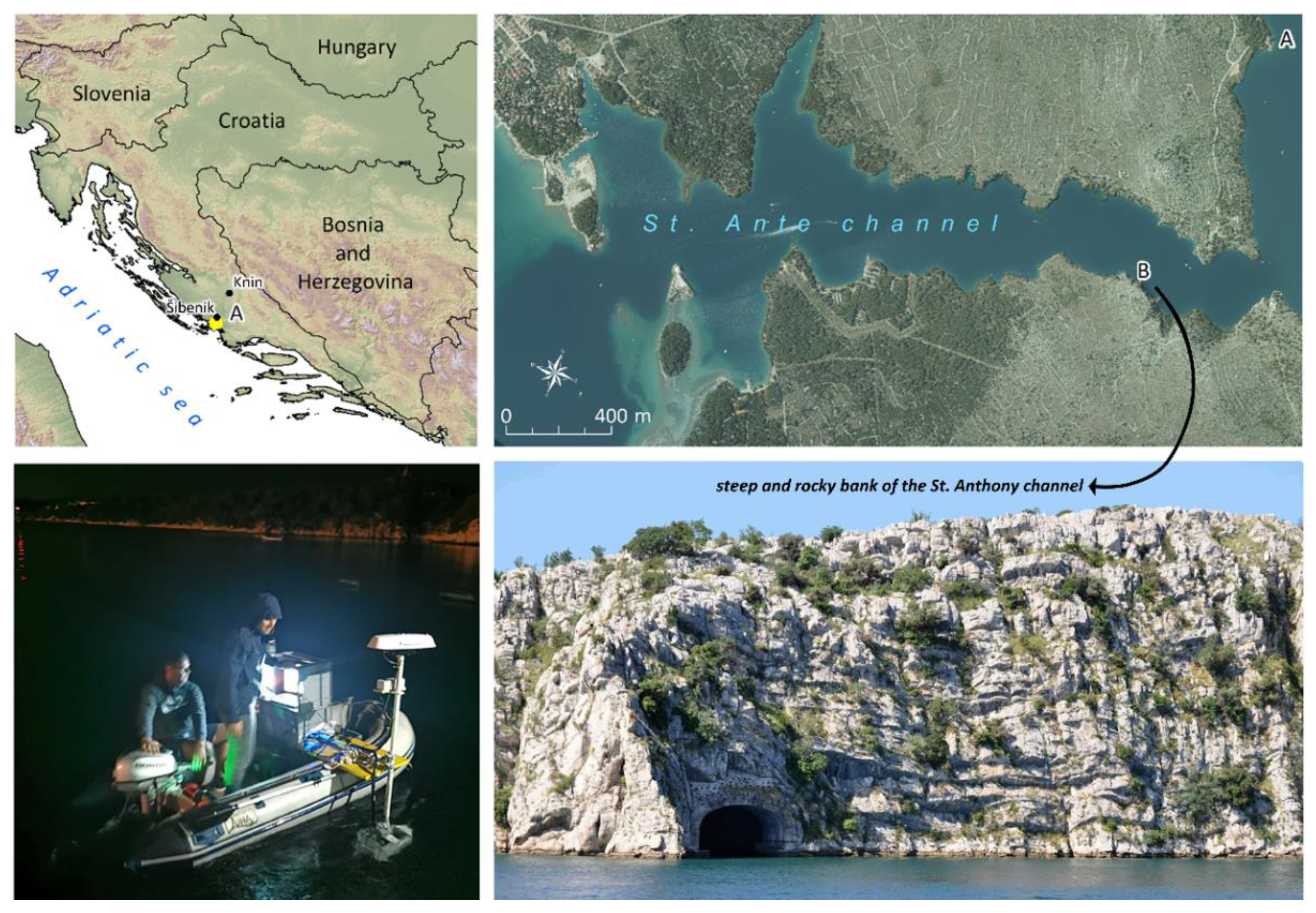
Study Area

2. Materials and Methods
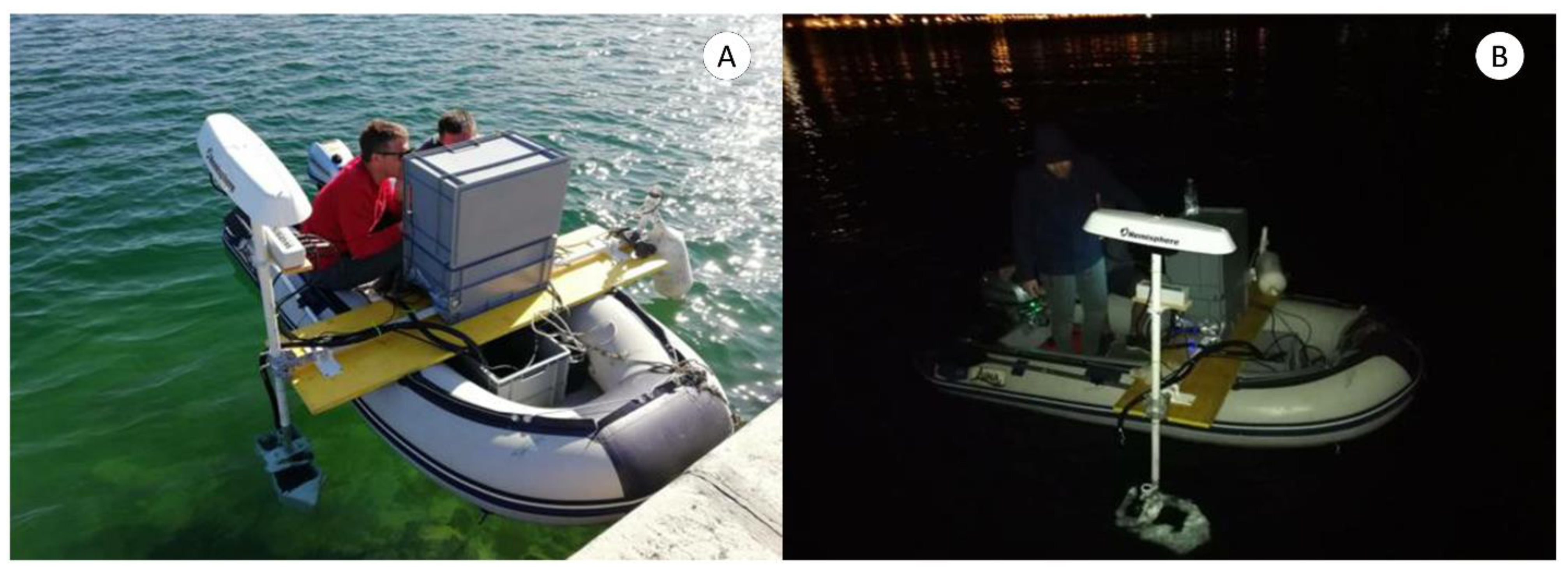
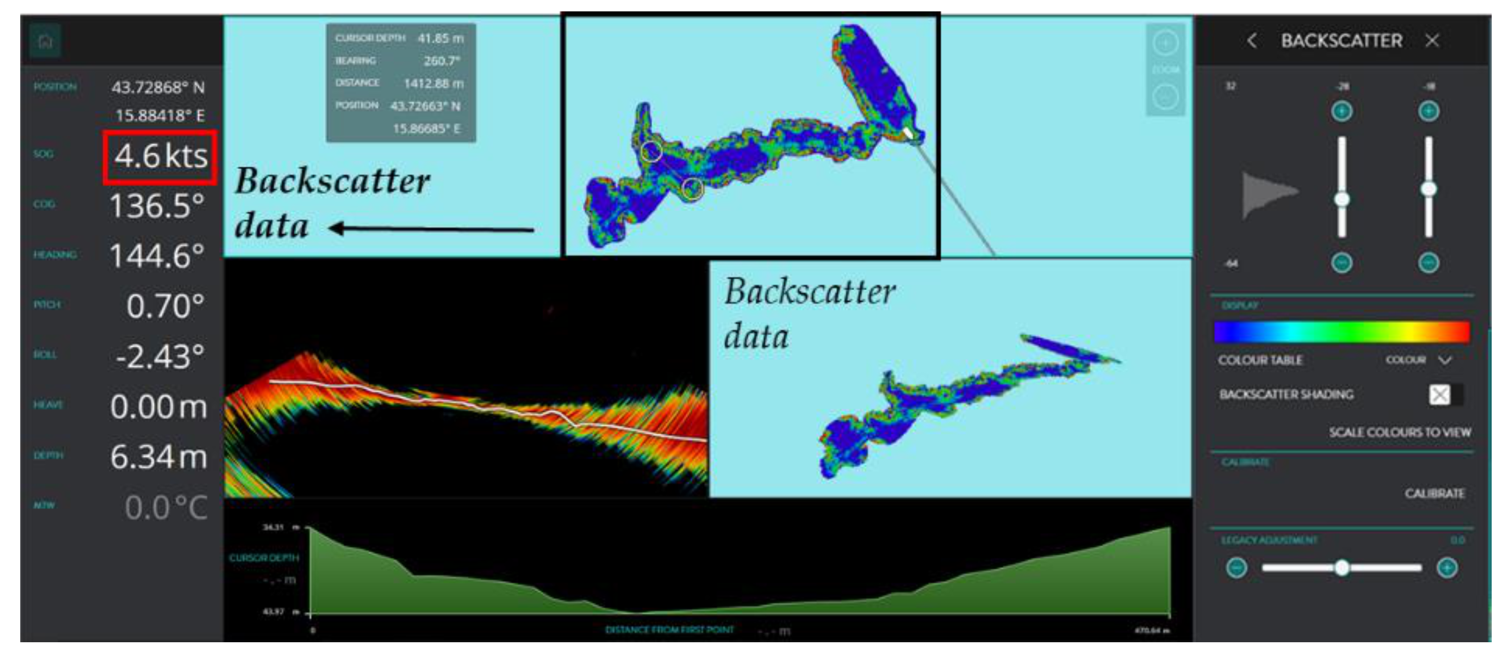
2.1. Multibeam Echosounder (MBES) Survey
- (1)
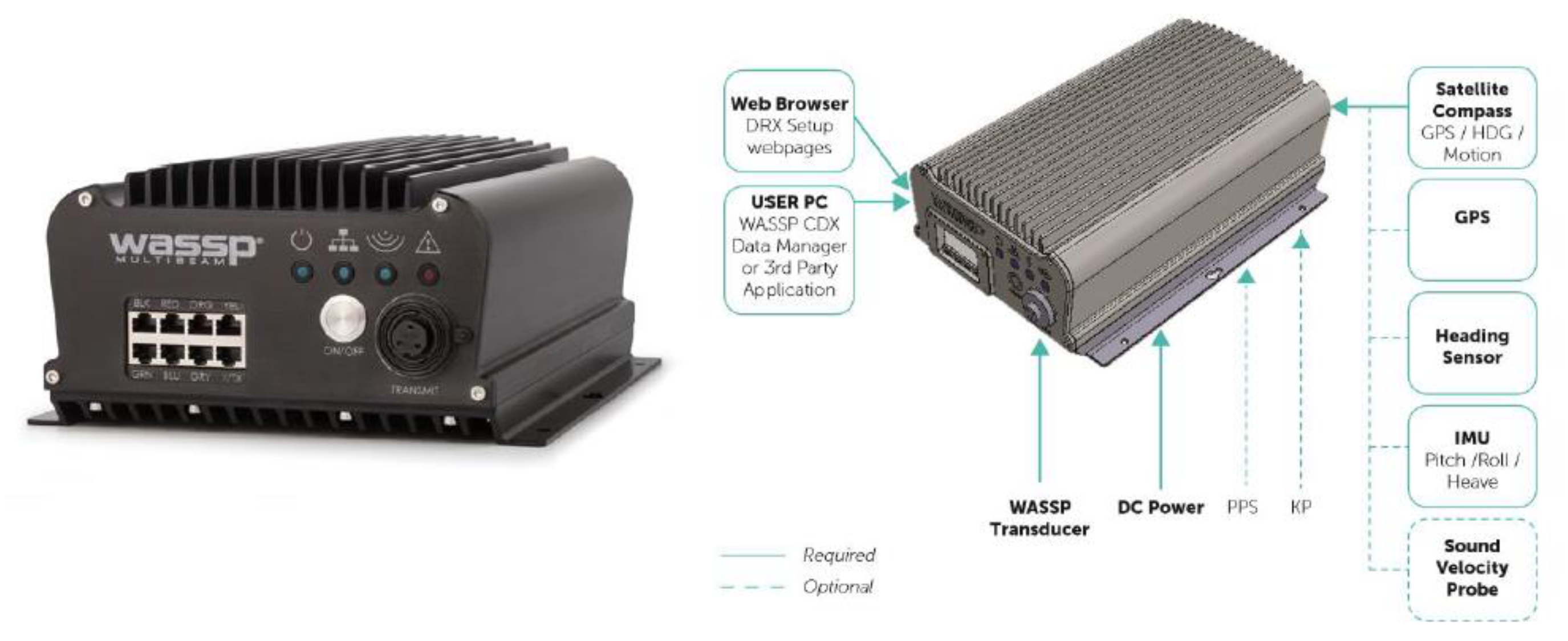
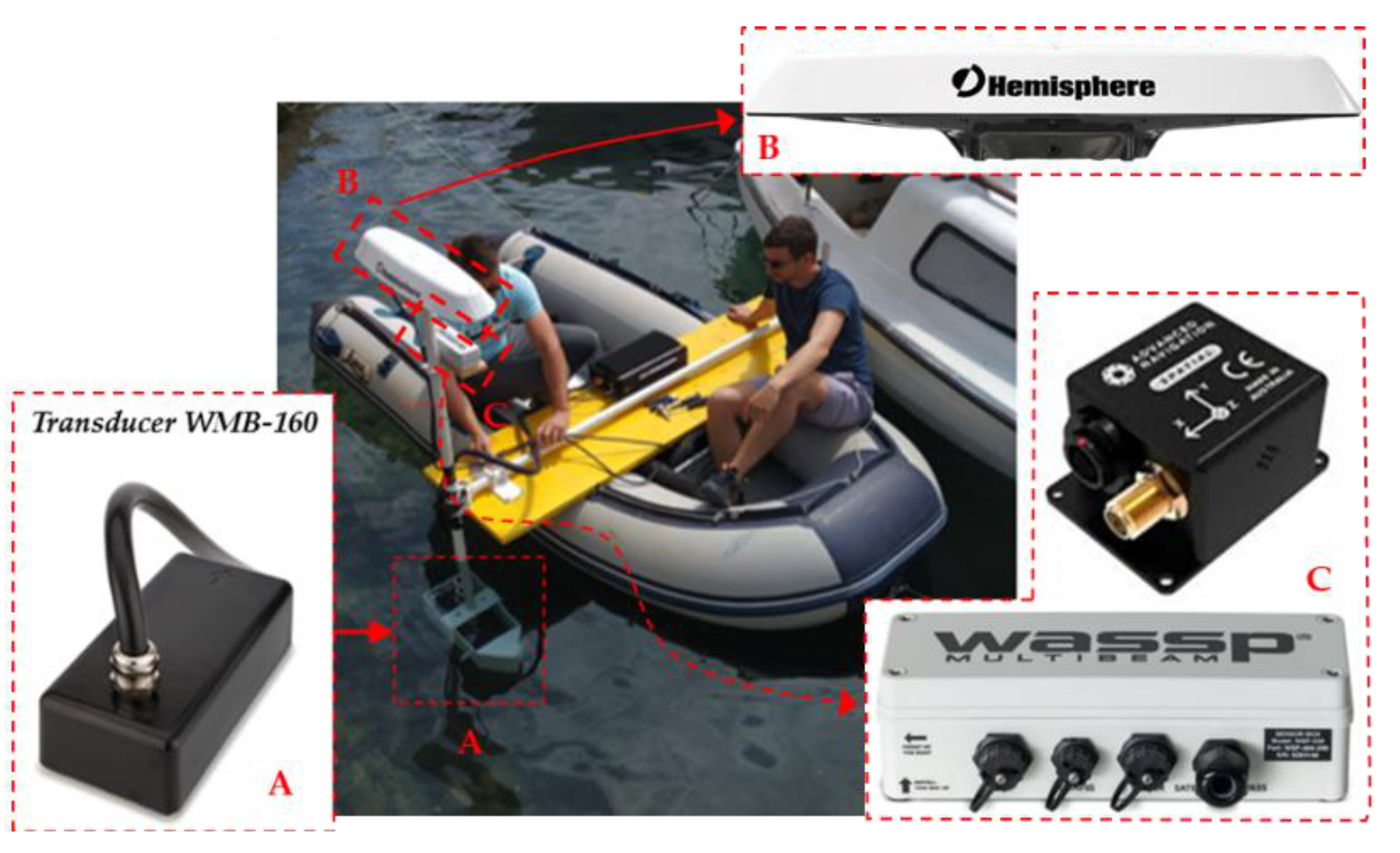
- WASSP S3 multibeam wideband sounder c/w DRX (Figure 4)
- (2)
- WASSP sensor box with integrated spatial IMU
- (3)
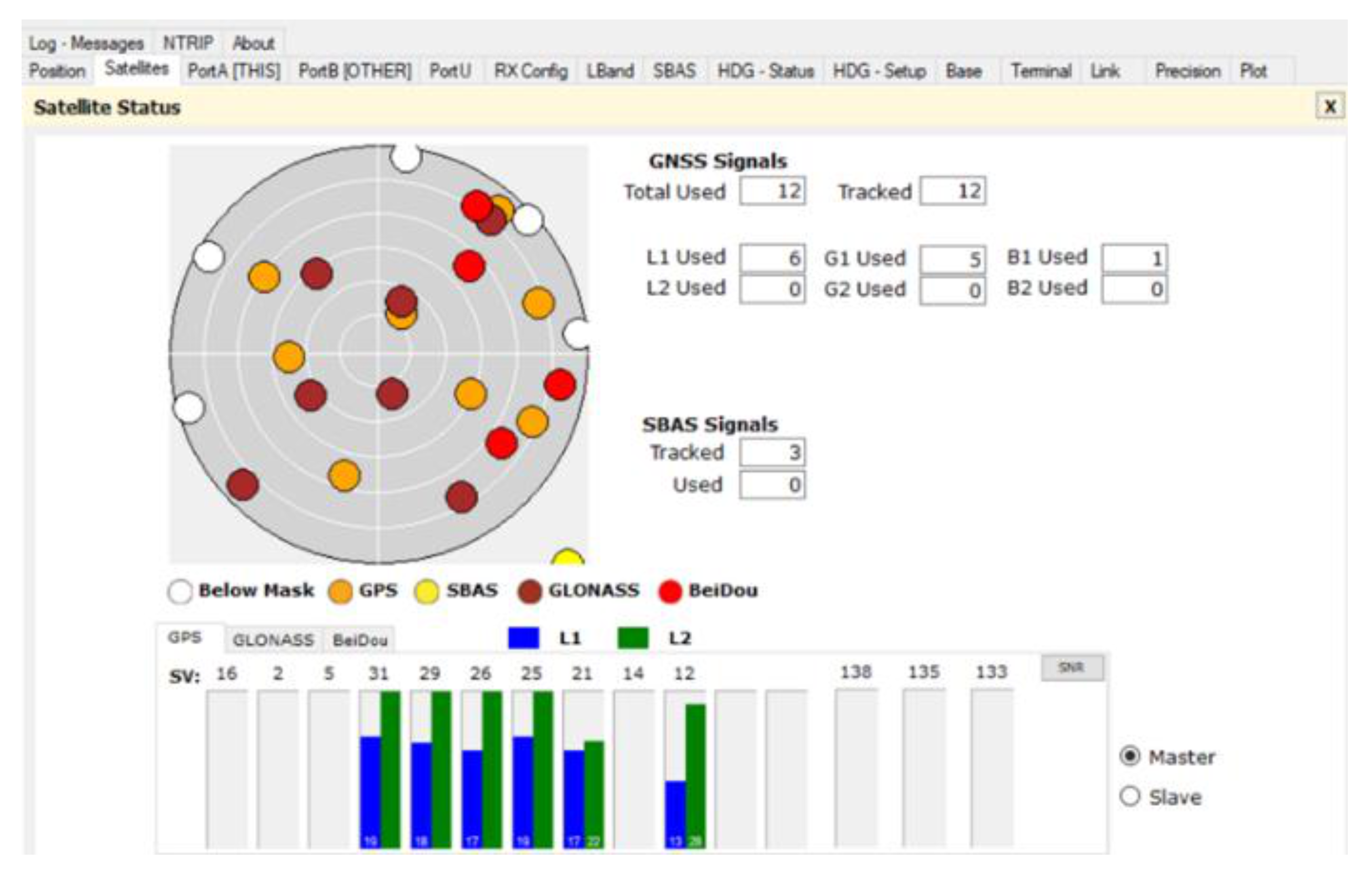
- Hemisphere V320 GNSS smart antenna (mFreq, mGNSS, RTK, SBAS)
- (4)
- accumulator and power cord
- (5)
- configuration computer and cable
- (6)
- configuration software (PoketMax, NtripClient, DRX Setup Webpages)
- (7)
- software for guidance (CDX) and data export (Data Manager)


| Receiver Type | Vector GNSS L1 Compass |
| Signals received | GPS and GLONASS |
| Channels | 502 |
| GPS sensitivity | −142 dBm |
| SBAS tracking | 3-channel, parallel tracking |
| Update rate timing (1 PPS) | 10 Hz standard, 20 Hz optional |
| Position accuracy: Single point | RMS (67%) 1.2 m; 2DRMS (95%) 2.5 m |
| Position accuracy: SBAS (WAAS) | RMS (67%) 0.3 m; 2DRMS (95%) 0.6 m |
| Position accuracy: Code differential GPS | RMS (67%) 0.3 m; 2DRMS (95%) 0.6 m |
| RTK | RMS (67%) 10 mm + 1 ppm; 2DRMS (95%) 20 mm + 2 ppm |
| Heading accuracy (RMS) | <0.17° |
| Heave accuracy (RMS) | <30 cm (DGNSS), <10 cm (RTK) |
| Pitch/Roll accuracy | <1° RMS |
| Timing (1 PPS) accuracy | 20 ns |
| Rate of turn | 100°/s maximum |
| Heading fix | 10 s typical (valid position) |
| Maximum speed | 1850 mph (999 kts) |
| Differential options | SBAS Beacon, External RTCM |
| L-Band Receiver Specifications | |
| Receiver type | Single channel |
| Channels | 1530 to 1560 MHz |
| Sensitivity | −130 dBm |
| Channel spacing | 5 kHz |
| Satellite selection | Manual or Automatic |
| Reacquisition time | 15 s (typical) |
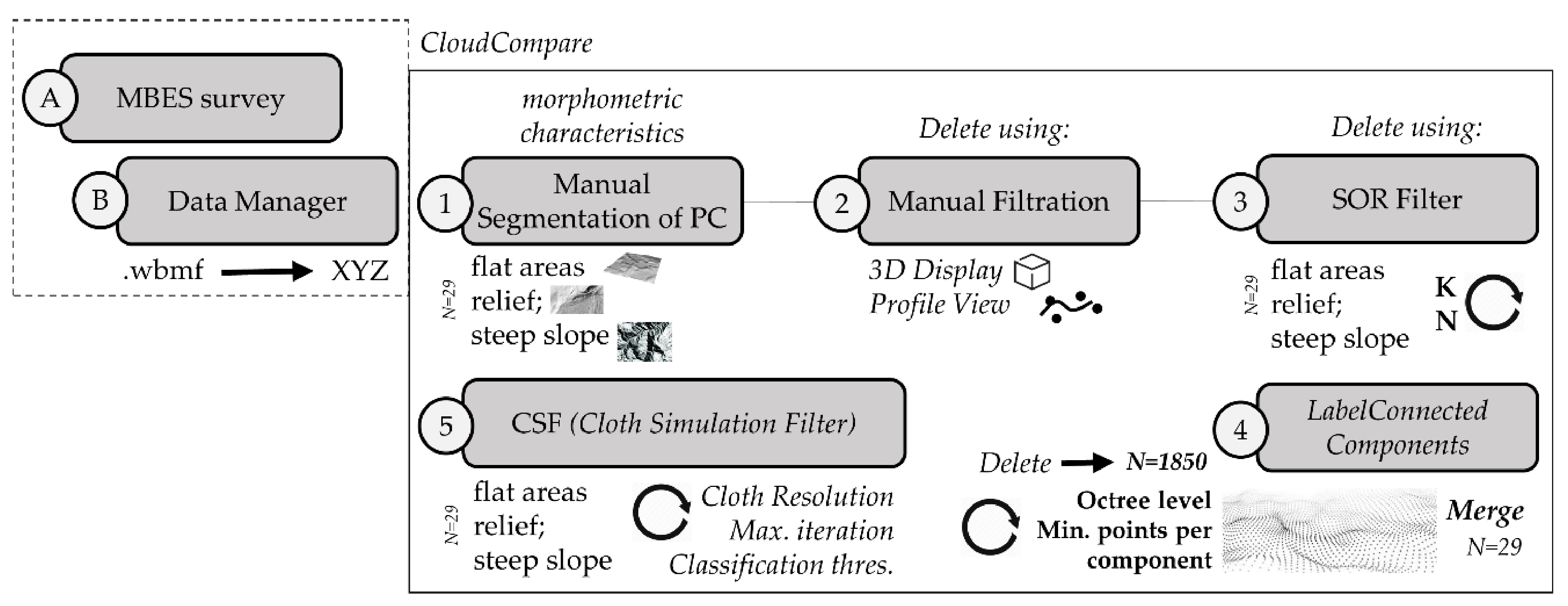
2.2. Data Processing
Point Filtering in CloudCompare (CC)
- (1)
- Manual segmentation of the point cloud;
- (2)
- Manual filtration using the 3D display and profile views;
- (3)
- SOR (Statistical Outlier Removal) filter;
- (4)
- Segmentation method (LabelConnected components);
- (5)
- CSF (Cloth Simulation Filter) method.

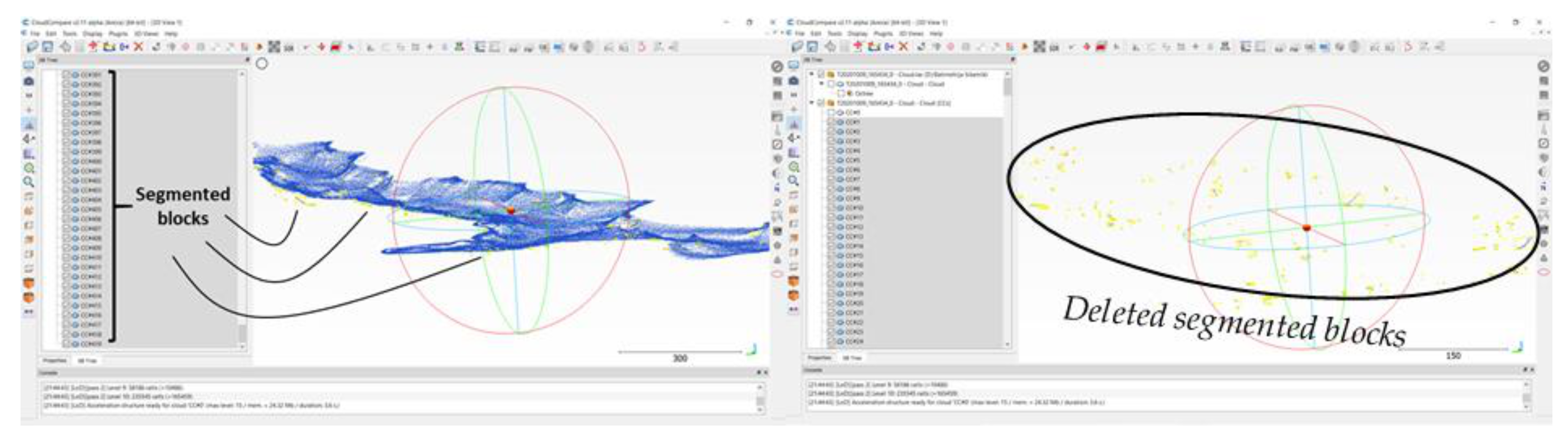
Manual Segmentation of the MBES Point Cloud
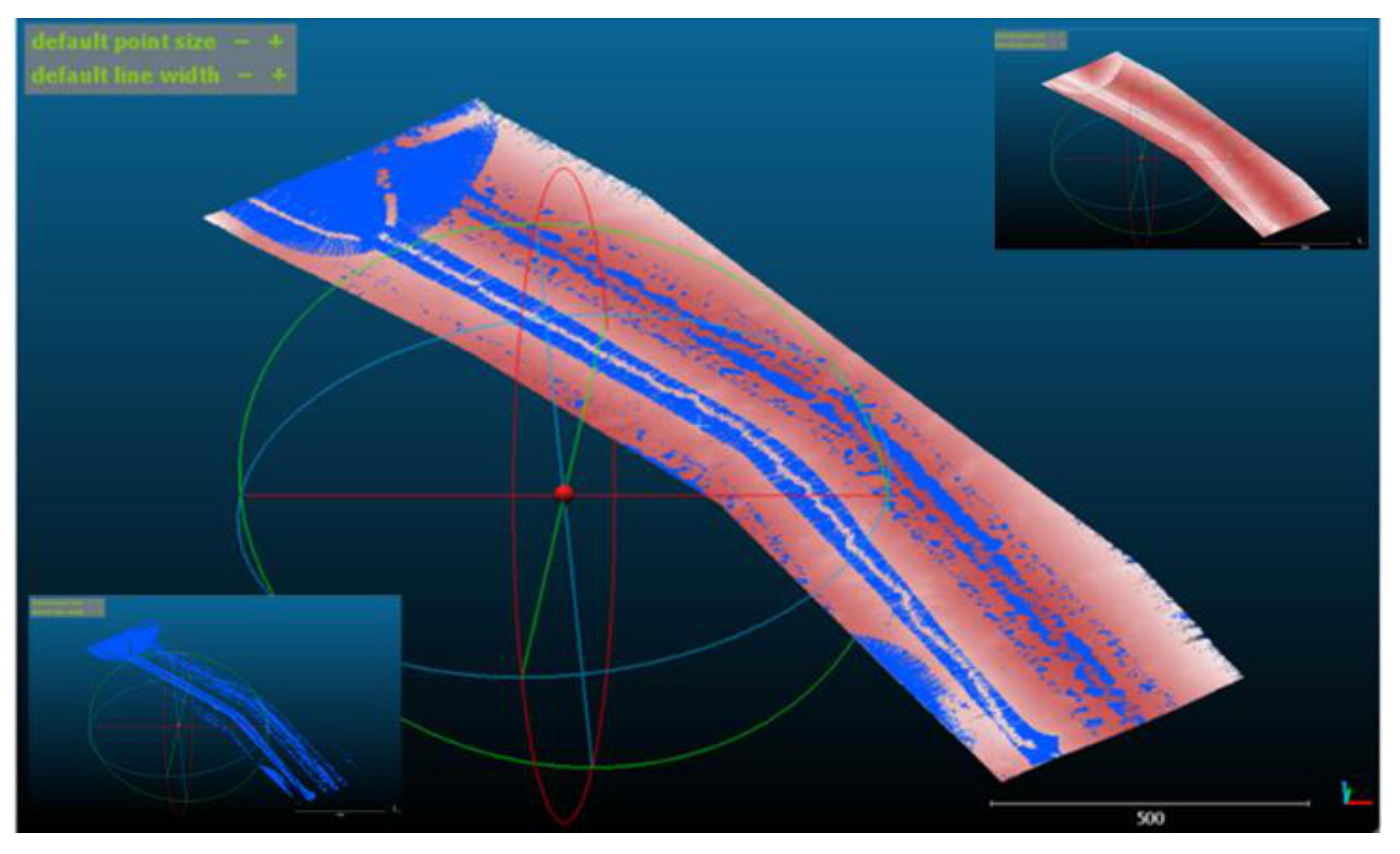
Manual Filtration Using the 3D Display and Profile View
SOR (Statistical Outlier Removal) Filter
LabelConnected Components
CSF (Cloth Simulation Filter) Filter
Creation of an Integrated Model of the St. Anthony Channel
3. Results
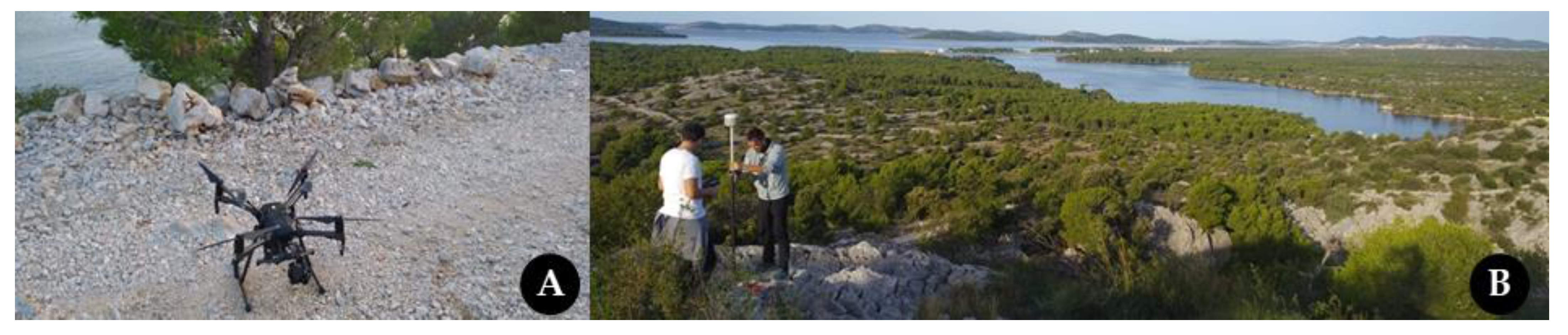
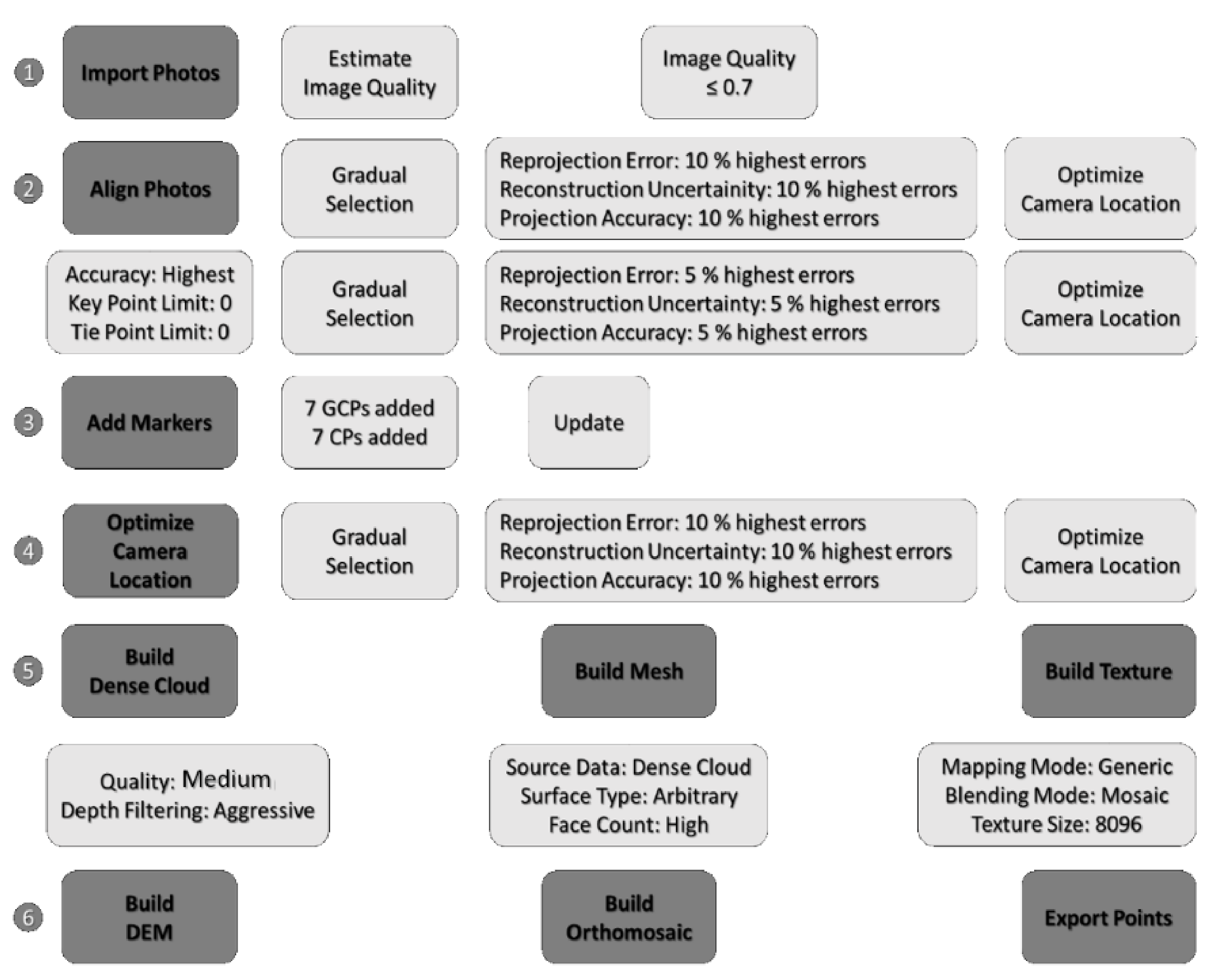
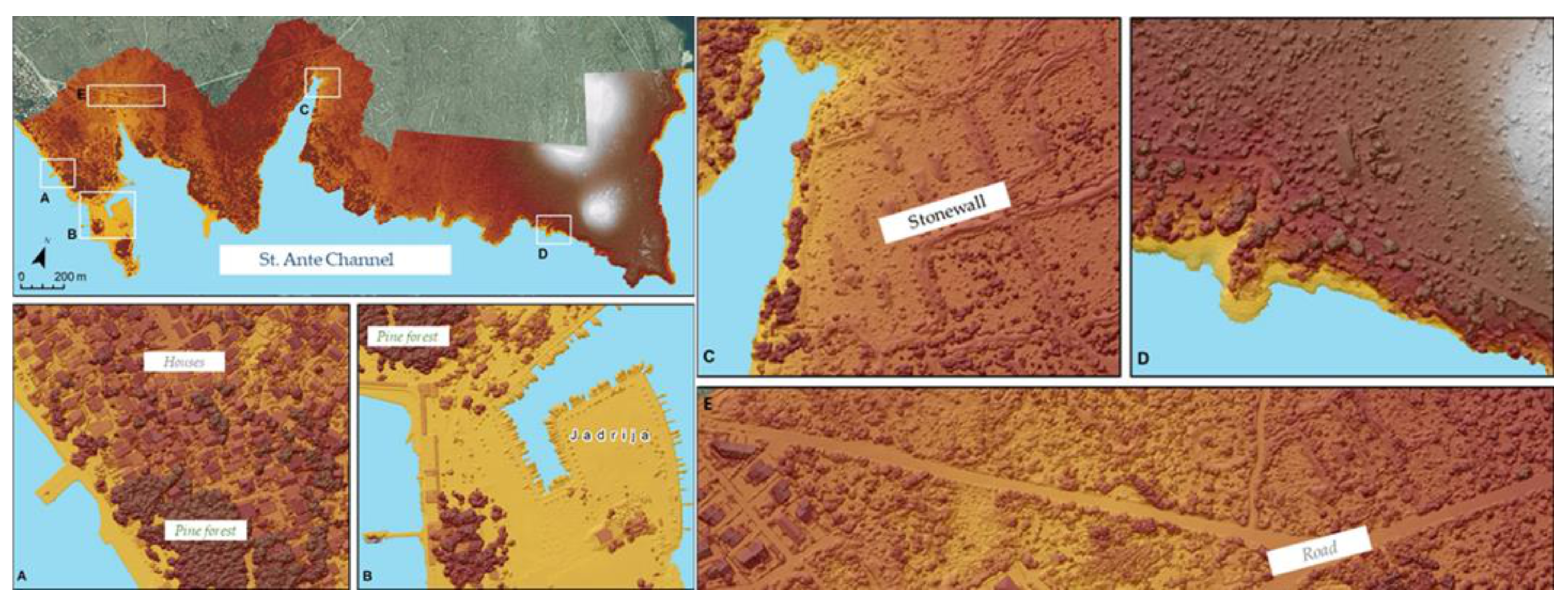
3.1. UAV Photogrammetry
3.2. Post-Processing Results of Acquired MBES Dataset
- (1)
- The manual segmentation of point cloud; and
- (2)
- Manual filtration using the 3D display and profile view.
- (3)
- SOR (Statistical Outlier Removal) filter.
- (4)
- Segmentation method (LabelConnected components).
- (5)
- CSF (Cloth Simulation Filter) method.
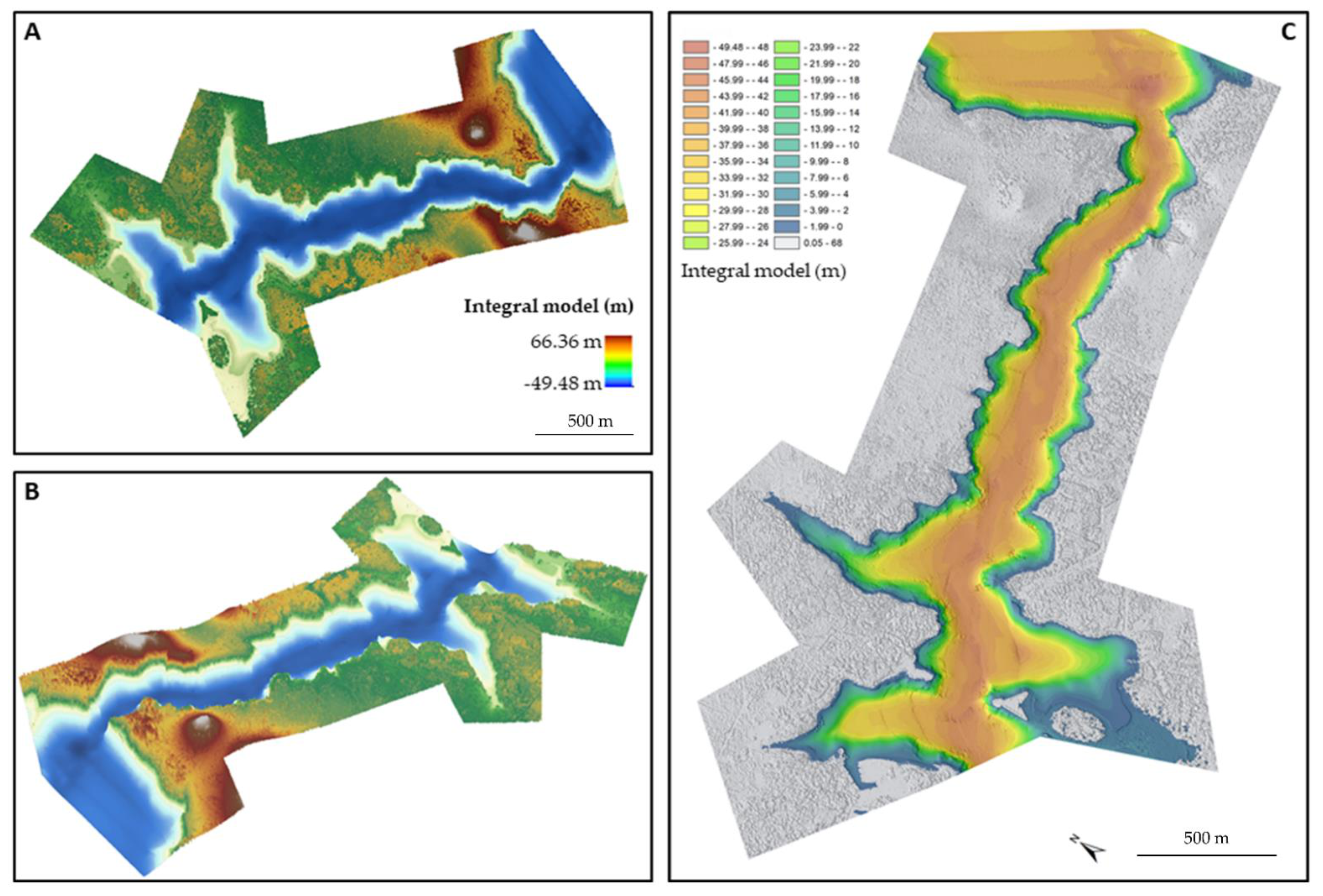
3.3. Integral (MBES and UAV) Model of the St. Anthony Channel

4. Conclusions
Author Contributions
Funding
Institutional Review Board Statement
Informed Consent Statement
Data Availability Statement
Acknowledgments
Conflicts of Interest
References
- Parnum, I.M.; Gavrilov, A.N. High-frequency multibeam echo-sounder measurements of seafloor backscatter in shallow water: Part 1–Data acquisition and processing. Underw. Technol. 2011, 30, 3–12. [Google Scholar] [CrossRef]
- Lecours, V.; Dolan, M.F.; Micallef, A.; Lucieer, V.L. A review of marine geomorphometry, the quantitative study of the seafloor. Hydrol. Earth Syst. Sci. 2016, 20, 3207. [Google Scholar] [CrossRef]
- Huizinga, R.J.; Heimann, D.C. Hydrographic Surveys of Rivers and Lakes Using a Multibeam Echosounder Mapping System; US Department of the Interior, US Geological Survey: Reston, VA, USA, 2018. [Google Scholar]
- Brown, C.J.; Beaudoin, J.; Brissette, M.; Gazzola, V. Multispectral multibeam echo sounder backscatter as a tool for improved seafloor characterization. Geosciences 2019, 9, 126. [Google Scholar] [CrossRef]
- Smith Menandro, P.; Cardoso Bastos, A. Seabed Mapping: A Brief History from Meaningful Words. Geosciences 2020, 10, 273. [Google Scholar] [CrossRef]
- Glenn, M.F. Introducing an operational multi-beam array sonar. Int. Hydrogr. Rev. 1970, 47, 35–39. [Google Scholar]
- Wölfl, A.C.; Snaith, H.; Amirebrahimi, S.; Devey, C.W.; Dorschel, B.; Ferrini, V.; Huvenne, V.A.I.; Jackobsson, M.; Jencks, J.; Johnston, G.; et al. Seafloor Mapping–the challenge of a truly global ocean bathymetry. Front. Mar. Sci. 2019, 6, 283. [Google Scholar] [CrossRef]
- Le Deunf, J.; Debese, N.; Schmitt, T.; Billot, R. A review of data cleaning approaches in a hydrographic framework with a focus on bathymetric multibeam echosounder datasets. Geosciences 2020, 10, 254. [Google Scholar] [CrossRef]
- Ierodiaconou, D.; Schimel, A.C.; Kennedy, D.; Monk, J.; Gaylard, G.; Young, M.; Diesing, M.; Rattray, A. Combining pixel and object based image analysis of ultra-high resolution multibeam bathymetry and backscatter for habitat mapping in shallow marine waters. Mar. Geophys. Res. 2018, 39, 271–288. [Google Scholar] [CrossRef]
- Brown, C.J. Benthic Habitat Mapping: From backscatter to biology. J. Ocean Technol. 2015, 10, 48–61. [Google Scholar]
- Gee, L.; Doucet, M.; Parker, D.; Weber, T.; Beaudoin, J. Is multibeam water column data really worth the disk space? In Proceedings of the Hydro12—Taking Care of the Sea, San Diego, CA, USA, 13–15 November 2012; pp. 13–15. [Google Scholar]
- Parnum, I.M.; Gavrilov, A.N.; Siwabessy, P.J.; Duncan, A.J. Analysis of high-frequency multibeam backscatter statistics from different seafloor habitats. In Proceedings of the Eighth European Conference on Underwater Acoustics, Carvoeiro, Portugal, 12–15 June 2006; pp. 775–780. [Google Scholar]
- Diesing, M. Application of geobia to map the seafloor. In Proceedings of the GEOBIA 2016: Solution and Synergies, ITC/University of Twente, Enschede, Netherlands, 14–16 September 2016; p. 3. [Google Scholar]
- Janowski, Ł.; Tęgowski, J.; Nowak, J. Seafloor mapping based on multibeam echosounder bathymetry and backscatter data using Object-Based Image Analysis: A case study from the Rewal site, the Southern Baltic. Oceanol. Hydrobiol. Stud. 2018, 47, 248–259. [Google Scholar] [CrossRef]
- Schimel, A.C.; Healy, T.R.; Johnson, D.; Immenga, D. Quantitative experimental comparison of single-beam, sidescan, and multibeam benthic habitat maps. ICES J. Mar. Sci. 2010, 67, 1766–1779. [Google Scholar] [CrossRef]
- Kjeldsen, K.K.; Weinrebe, R.W.; Bendtsen, J.; Bjørk, A.A.; Kjær, K.H. Multibeam bathymetry and CTD measurements in two fjord systems in southeastern Greenland. Earth Sci. Data 2017, 9, 589–600. [Google Scholar] [CrossRef]
- Šiljeg, A.; Cavrić, B.; Marić, I.; Barada, M. GIS modelling of bathymetric data in the construction of port terminals–An example of Vlaška channel in the Port of Ploče, Croatia. Int. J. Eng. Model. 2019, 32, 17–37. [Google Scholar] [CrossRef]
- Amirebrahimi, S.; Picard, K.; Quadros, N.; Falster, G. Multibeam Echo Sounder Data Acquisition in Australia and Beyond—User Needs Summary. Geosci. Aust. Rec. 2019, 8, 47. [Google Scholar]
- Kostylev, V.E.; Todd, B.J.; Fader, G.B.J.; Courtney, R.C.; Cameron, G.D.M.; Pickrill, R.A. Benthic habitat mapping on the Scotian Shelf based on multibeam bathymetry, surficial geology and sea floor photographs. Mar. Ecol. Prog. Ser. 2001, 219, 121–137. [Google Scholar] [CrossRef]
- Brown, C.J.; Smith, S.J.; Lawton, P.; Anderson, J.T. Benthic habitat mapping: A review of progress towards improved understanding of the spatial ecology of the seafloor using acoustic techniques. Estuar. Coast. Shelf Sci. 2011, 92, 502–520. [Google Scholar] [CrossRef]
- Kostylev, V.E.; Courtney, R.C.; Robert, G.; Todd, B.J. Stock evaluation of giant scallop (Placopecten magellanicus) using high-resolution acoustics for seabed mapping. Fish. Res. 2003, 60, 479–492. [Google Scholar] [CrossRef]
- Šiljeg, A.; Marić, I.; Roland, V. Izrada tematskih karata na temelju podataka prikupljenih batimetrijskom izmjerom. Zbornik radova: Vizija i izazovi upravljanja zaštićenim područjima prirode u Republici Hrvatskoj-Aktivna zaštita i održivo upravljanje u Nacionalnom parku “Krka”/Marguš, Drago (ur.). Šibenik Javna Ustanov. 2017, 1, 994–1016. [Google Scholar]
- Madricardo, F.; Foglini, F.; Kruss, A.; Ferrarin, C.; Pizzeghello, N.M.; Murri, C.; Rossi, M.; Bajo, M.; Bellafiore, D.; Campiani, E.; et al. High resolution multibeam and hydrodynamic datasets of tidal channels and inlets of the Venice Lagoon. Sci. Data 2017, 4, 170121. [Google Scholar] [CrossRef]
- Vogt, P.R.; Smoot, N.C. The Geisha Guyots: Multibeam bathymetry and morphometric interpretation. J. Geophys. Res. Solid Earth 1984, 89, 11085–11107. [Google Scholar] [CrossRef]
- Lawver, L.A.; Sloan, B.J.; Barker, D.H.; Ghidella, M.; Von Herzen, R.P.; Keller, R.A.; Klinkhammer, G.P.; Chin, C.S. Distributed, active extension in Bransfield Basin, Antarctic Peninsula: Evidence from multibeam bathymetry. GSA Today 1996, 6, 1–6. [Google Scholar]
- Wilson, M.F.J.; O’Connell, B.; Brown, C.; Guinan, J.C.; Grehan, A.J. Multiscale Terrain Analysis of Multibeam Bathymetry Data for Habitat Mapping on the Continental Slope. Mar. Geod. 2007, 30, 3–35. [Google Scholar] [CrossRef]
- Dartnell, P.; Gardner, J.V. Predicting seafloor facies from multibeam bathymetry and backscatter data. Photogramm. Eng. Remote Sens. 2004, 70, 1081–1091. [Google Scholar] [CrossRef]
- Bentrem, F.W.; Avera, W.E.; Sample, J. Estimating surface sediments using multibeam sonar. arXiv 2006, arXiv:0606191. [Google Scholar]
- Moore, C.H.; Harvey, E.S.; Van Niel, K.P. Spatial prediction of demersal fish distributions: Enhancing our understanding of species—Environment relationships. ICES J. Mar. Sci. 2009, 66, 2068–2075. [Google Scholar] [CrossRef]
- Hasan, R.C.; Ierodiaconou, D.; Rattray, A.; Monk, J.; Laurenson, L. Applications of multibeam echosounder data and video observations for biological monitoring on the south east Australian continental shelf. In Proceedings of the International Symposium and Exhibition on Geoinformation, Shah Alam, Malaysia, 27–29 September 2011; pp. 1–16. [Google Scholar]
- Quinn, R.J.; Dix, J.K.; Dean, M. Chapter 13: Geophysical and remote sensing surveys. In Archaeology Underwater: The Nautical Archaeology Society Guide to Principles and Practice, 2nd ed.; Bowens, A., Ed.; Wiley-Blackwell: Oxford, UK, 2008. [Google Scholar]
- Westley, K.; Quinn, R.; Forsythe, W.; Plets, R.; Bell, T.; Benetti, S.; McGrath, F.; Robinson, R. Mapping submerged landscapes using multibeam bathymetric data: A case study from the north coast of Ireland. Int. J. Naut. Archaeol. 2011, 40, 99–112. [Google Scholar] [CrossRef]
- Plets, R.; Quinn, R.; Forsythe, W.; Westley, K.; Bell, T.; Benetti, S.; McGrath, F.; Robinson, R. Using multibeam echo-sounder data to identify shipwreck sites: Archaeological assessment of the joint Irish bathymetric survey data. Int. J. Naut. Archaeol. 2011, 40, 87–98. [Google Scholar] [CrossRef]
- Kan, H.; Katagiri, C.; Nakanishi, Y.; Yoshizaki, S.; Nagao, M.; Ono, R. Assessment and Significance of a World War II battle site: Recording the USS Emmons using a High-Resolution DEM combining Multibeam Bathymetry and SfM Photogrammetry. Int. J. Naut. Archaeol. 2018, 47, 267–280. [Google Scholar] [CrossRef]
- Pydyn, A.; Popek, M.; Kubacka, M.; Janowski, Ł. Exploration and reconstruction of a medieval harbour using hydroacoustics, 3-D shallow seismic and underwater photogrammetry: A case study from Puck, southern Baltic Sea. Archaeol. Prospect. 2021, 28, 527–542. [Google Scholar] [CrossRef]
- Madricardo, F.; Bassani, M.; D’Acunto, G.; Calandriello, A.; Foglini, F. New evidence of a Roman road in the Venice Lagoon (Italy) based on high resolution seafloor reconstruction. Sci. Rep. 2021, 11, 1–19. [Google Scholar]
- Bosman, A.; Romagnoli, C.; Madricardo, F.; Correggiari, A.; Remia, A.; Zubalich, R.; Fogarin, S.; Kruss, A.; Trincardi, F. Short-term evolution of Po della Pila delta lobe from time lapse high-resolution multibeam bathymetry (2013–2016). Estuar. Coast. Shelf Sci. 2020, 233, 106533. [Google Scholar] [CrossRef]
- Pillay, T.; Cawthra, H.C.; Lombard, A.T. Characterisation of seafloor substrate using advanced processing of multibeam bathymetry, backscatter, and sidescan sonar in Table Bay, South Africa. Mar. Geol. 2020, 429, 106332. [Google Scholar] [CrossRef]
- Chiocci, F.L.; Cattaneo, A.; Urgeles, R. Seafloor mapping for geohazard assessment: State of the art. Mar. Geophys. Res. 2011, 32, 1–11. [Google Scholar] [CrossRef]
- Fenty, I.; Willis, J.K.; Khazendar, A.; Dinardo, S.; Forsberg, R.; Fukumori, I.; Holland, D.; Jakobsson, M.; Moller, D.; Morison, J.; et al. Oceans Melting Greenland: Early results from NASA’s ocean-ice mission in Greenland. Oceanography 2016, 29, 72–83. [Google Scholar] [CrossRef]
- Gula, J.; Molemaker, M.J.; McWilliams, J.C. Gulf Stream dynamics along the southeastern US seaboard. J. Phys. Oceanogr. 2015, 45, 690–715. [Google Scholar] [CrossRef]
- Ellis, J.I.; Clark, M.R.; Rouse, H.L.; Lamarche, G. Environmental management frameworks for offshore mining: The New Zealand approach. Mar. Policy 2017, 84, 178–192. [Google Scholar] [CrossRef][Green Version]
- Nasby-Lucas, N.M.; Embley, B.W.; Hixon, M.A.; Merle, S.G.; Tissot, B.N.; Wright, D.J. Integration of submersible transect data and high-resolution multibeam sonar imagery for a habitat-based groundfish assessment of Heceta Bank. Fish Bull. 2002, 100, 739–751. [Google Scholar]
- Hein, J.R.; Conrad, T.A.; Dunham, R.E. Seamount characteristics and mine-site model applied to exploration-and mining-lease-block selection for cobalt-rich ferromanganese crusts. Mar. Georesources Geotechnol. 2009, 27, 160–176. [Google Scholar] [CrossRef]
- Rengstorf, A.M.; Mohn, C.; Brown, C.; Wisz, M.S.; Grehan, A.J. Predicting the distribution of deep-sea vulnerable marine ecosystems using high-resolution data: Considerations and novel approaches. Deep. Sea Res. Part I Oceanogr. Res. Pap. 2014, 93, 72–82. [Google Scholar] [CrossRef]
- Jordan, A.; Lawler, M.; Halley, V.; Barrett, N. Seabed habitat mapping in the Kent Group of islands and its role in marine protected area planning. Aquat. Conserv. Mar. Freshw. Ecosyst. 2005, 15, 51–70. [Google Scholar] [CrossRef]
- Micallef, A.; Foglini, F.; Le Bas, T.; Angeletti, L.; Maselli, V.; Pasuto, A.; Taviani, M. The submerged paleolandscape of the Maltese Islands: Morphology, evolution and relation to Quaternary environmental change. Mar. Geol. 2013, 335, 129–147. [Google Scholar] [CrossRef]
- Kulawiak, M.; Lubniewski, Z. Processing of LiDAR and multibeam sonar point cloud data for 3D surface and object shape reconstruction. In Proceedings of the 2016 Baltic Geodetic Congress (BGC Geomatics), Gdansk, Poland, 2–4 June 2016; IEEE: Gdansk, Poland, 2016; pp. 187–190. [Google Scholar]
- Moszynski, M.; Chybicki, A.; Kulawiak, M.; Lubniewski, Z. A novel method for archiving multibeam sonar data with emphasis on efficient record size reduction and storage. Pol. Marit. Res. 2013, 20, 77–86. [Google Scholar] [CrossRef]
- Nathalie, D.; Thierry, S.; François, G.; Etienne, J.; Lucas, V.; Romain, B. Outlier detection for Multibeam echo sounder (MBES) data: From past to present. In Proceedings of the IEEE Oceans 2019, Marseille, France, 17–20 June 2019; pp. 1–10. [Google Scholar]
- Ferreira, I.O.; Santos, A.D.P.D.; Oliveira, J.C.D.; Medeiros, N.D.G.; Emiliano, P.C. Robust methodology for detection of spikes in multibeam echo sounder data. Bol. Ciências Geodésicas 2019, 25, e2019014. [Google Scholar] [CrossRef]
- Makar, A. Algorithms for Cleaning the Data Recorded by Multibeam Echosounder. In International Conference on Geo Sciences GEOLINKS 2019; Saima Consult LTD: Athens, Greece, 2019; Volume 1, pp. 259–266. [Google Scholar]
- Stevens, A.H.; Butkiewicz, T. Faster Multibeam Sonar Data Cleaning: Evaluation of Editing 3D Point Clouds using Immersive VR. In Proceedings of the OCEANS 2019 MTS/IEEE, Seattle, WA, USA, 27–31 October 2019; IEEE: Seattle, WA, USA, 2019; pp. 1–10. [Google Scholar]
- Arge, L.; Larsen, K.G.; Mølhave, T.; van Walderveen, F. Cleaning massive sonar point clouds. In Proceedings of the 18th SIGSPATIAL International Conference on Advances in Geographic Information Systems, San Jose, CA, USA, 2–5 November 2010; pp. 152–161. [Google Scholar]
- Rakotosaona, M.J.; La Barbera, V.; Guerrero, P.; Mitra, N.J.; Ovsjanikov, M. Pointcleannet: Learning to denoise and remove outliers from dense point clouds. Comput. Graph. Forum 2020, 39, 185–203. [Google Scholar] [CrossRef]
- Chen, C.; Gawel, A.; Krauss, S.; Zou, Y.; Abbott, A.L.; Stilwell, D.J. Robust Unsupervised Cleaning of Underwater Bathymetric Point Cloud Data. In Proceedings of the 31st British Machine Vision Virtual Conference, Online, 7–10 September 2020. [Google Scholar]
- Hodge, V.; Austin, J. A survey of outlier detection methodologies. Artif. Intell. Rev. 2004, 22, 85–126. [Google Scholar] [CrossRef]
- Santos, A.M.R.T.; Santos, G.R.D.; Emiliano, P.C.; Medeiros, N.D.G.; Kaleita, A.L.; Pruski, L.D.O.S. Detection of inconsistencies in geospatial data with geostatistics. Bol. De Ciências Geodésicas 2017, 23, 296–308. [Google Scholar] [CrossRef]
- Debese, N. Bathymétrie-Sondeurs, Traitement des Données Modèles Numériques de Terrain-Cours Exercices Corrigés; Ellipses: Paris, France, 2013. [Google Scholar]
- Calder, B.R.; Mayer, L.A. Automatic processing of high-rate, high-density multibeam echosounder data. Geochem. Geophys. Geosyst. 2003, 4, 1–22. [Google Scholar] [CrossRef]
- Calder, B.R. Automatic statistical processing of multibeam echosounder data. Int. Hydro. Rev. 2003, 4, 36–52. [Google Scholar]
- Vaaja, M.; Kukko, A.; Kaartinen, H.; Kurkela, M.; Kasvi, E.; Flener, C.; Hyyppä, H.; Järvelä, J.; Alho, P. Data processing and quality evaluation of a boat-based mobile laser scanning system. Sensors 2013, 13, 12497–12515. [Google Scholar] [CrossRef]
- Carić, H.; Cukrov, N.; Omanović, D. Nautical Tourism in Marine Protected Areas (MPAs): Evaluating an Impact of Copper Emission from Antifouling Coating. Sustainability 2021, 13, 11897. [Google Scholar] [CrossRef]
- Belamarić, G.; Kurtela, Ž.; Bošnjak, R. Simulation method-based oil spill pollution risk analysis for the port of šibenik. Trans. Marit. Sci. 2016, 5, 141–154. [Google Scholar] [CrossRef][Green Version]
- Lovrinčević, D. Quality assessment of an automatic sounding selection process for navigational charts. Cartogr. J. 2017, 5, 139–146. [Google Scholar] [CrossRef]
- IHB. Manual on Hydrography Publication C-13, 1st ed.; International Hydrographic Bureau: Monte Carlo, Monaco, 2005. [Google Scholar]
- Weatherall, P.; Marks, K.M.; Jakobsson, M.; Schmitt, T.; Tani, S.; Arndt, J.E.; Rovere, M.; Chayes, D.; Ferrini, V.; Wigley, R. A new digital bathymetric model of the world’s oceans. Earth Space Sci. 2015, 2, 331–345. [Google Scholar] [CrossRef]
- Hell, B.; Broman, B.; Jakobsson, L.; Jakobsson, M.; Magnusson, Å.; Wiberg, P. The use of bathymetric data in society and science: A review from the Baltic Sea. Ambio 2012, 41, 138–150. [Google Scholar] [CrossRef] [PubMed]
- Geomatching. Multibeam EchoScounder. Available online: https://geo-matching.com/multibeam-echosounders (accessed on 29 November 2021).
- Wassp Multibeam. Available online: https://www.enl.co.nz/pages/wassp-s3 (accessed on 29 November 2021).
- Nugraha, W.; Parapat, A.D.; Arum, D.S.; Istighfarini, F. GNSS RTK Application to Determine Coastline Case Study at Northen Area of Sulawesi and Gorontalo. E3S Web Conf. 2019, 94, 01016. [Google Scholar] [CrossRef]
- Hemisphere GNSS. Vector V320 GNSS Smart Antenna User Guide Part No. 875-0351-0 Rev. A1. 2015. Available online: https://hemispheregnss.com/wp-content/uploads/2018/12/hemispheregnss_v320_ug_userguide_875-0351-0_a1-1.pdf (accessed on 9 December 2020).
- Šantek, D. Ispitivanje CROPOS-a. Geod. List. 2013, 67, 281–297. [Google Scholar]
- Montereale-Gavazzi, G.; Roche, M.; Lurton, X.; Degrendele, K.; Terseleer, N.; Van Lancker, V. Seafloor change detection using multibeam echosounder backscatter: Case study on the Belgian part of the North Sea. Mar. Geophys. Res. 2018, 39, 229–247. [Google Scholar] [CrossRef]
- YSI, EXO2 Multiparameter Sond. Available online: https://www.ysi.com/exo2 (accessed on 29 November 2021).
- Dong, Q.L.; Cui, M.X.; Zhou, J.H.; Wang, J.G.; Xu, Y. Analysis and Processing of Transform Geography of Convex and Cave in Multibeam Sounding System. Hydrogr. Surv. Charting 2011, 1, 32–35. [Google Scholar]
- Dong, Q.L.; Han, H.Q.; Fang, Z.B.; Pan, L.; Chen, Y.Y.; Lu, G.F. The Influence of Sound Speed Profiles Correction on Multi-beam Survey. Hydrogr. Surv. Charting 2007, 2, 56–58. [Google Scholar]
- CloudCompare, CloudCompare 3D Point Cloud and Mesh Processing Software Open Source Project. Available online: https://cloudcompare.org (accessed on 20 August 2020).
- Skinner, B.; Vidal-Calleja, T.; Miro, J.V.; De Bruijn, F.; Falque, R. 3D point cloud upsampling for accurate reconstruction of dense 2.5 D thickness maps. In Proceedings of the Australasian Conference on Robotics and Automation, ACRA, Melbourne, Australia, 2–4 December 2014. [Google Scholar]
- Charron, N.; Phillips, S.; Waslander, S.L. De-noising of lidar point clouds corrupted by snowfall. In Proceedings of the 2018 15th Conference on Computer and Robot Vision (CRV), Toronto, ON, Canada, 9–11 May 2018; pp. 254–261. [Google Scholar]
- Ruchay, A.N.; Dorofeev, K.A.; Kalschikov, V.V. Accuracy analysis of 3D object reconstruction using point cloud filtering algorithms. In Proceedings of the 5th Information Technology and Nanotechnology, ITNT-2019, Samara, Russia, 21–24 May 2019. [Google Scholar]
- Abdelazeem, M.; Elamin, A.; Afifi, A.; El-Rabbany, A. Multi-sensor point cloud data fusion for precise 3D mapping. Egypt. J. Remote Sens. Space Sci. 2021, 24, 835–844. [Google Scholar] [CrossRef]
- Zeybek, M. Inlier Point Preservation in Outlier Points Removed from the ALS Point Cloud. J. Indian Soc. Remote Sens. 2021, 49, 2347–2363. [Google Scholar] [CrossRef]
- Carrilho, A.C.; Galo, M.; Santos, R.C. Statistical outlier detection method for airborne lidar data. In Proceedings of the International Archives of the Photogrammetry, Remote Sensing and Spatial Information Sciences, Volume XLII-1, ISPRS TC I Mid-term Symposium “Innovative Sensing—From Sensors to Methods and Applications”, Karlsruhe, Germany, 10–12 October 2018. [Google Scholar]
- Chen, S.; Truong-Hong, L.; O’Keeffe, E.; Laefer, D.F.; Mangina, E. Outlier detection of point clouds generating from low cost UAVs for bridge inspection. In Life-Cycle Analysis and Assessment in Civil Engineering: Towards an Integrated Vision; Caspeele, R., Taerwe, L., Frangopol, D.M., Eds.; CRC Press: Ghent, Belgium, 2018. [Google Scholar]
- Kharroubi, A.; Hajji, R.; Billen, R.; Poux, F. Classification and integration of massive 3d points clouds in a virtual reality (VR) environment. International Archives of the Photogrammetry. Remote Sens. Spat. Inf. Sci. 2019, 42, 165–171. [Google Scholar]
- CloudCompare, Label Connected Components. Available online: https://www.cloudcompare.org/doc/wiki/index.php?title=Label_Connected_Components (accessed on 14 December 2020).
- Kaňuk, J.; Šupinský, J.; Šašak, J.; Hofierka, J.; Wang, Y.; Zhang, Q.; Sedlák, V.; Onačillová, K.; Gallay, M. Semi-automatic LiDAR point cloud denoising using a connected-component labelling method. Geogr. Cassoviensis 2019, 13, 210–227. [Google Scholar] [CrossRef]
- Cai, S.; Zhang, W.; Liang, X.; Wan, P.; Qi, J.; Yu, S.; Yan, G.; Shao, J. Filtering airborne LiDAR data through complementary cloth simulation and progressive TIN densification filters. Remote Sens. 2019, 11, 1037. [Google Scholar] [CrossRef]
- Lee, J.B.; Jung, J.H.; Kim, H.J. Segmentation of Seabed Points from Airborne Bathymetric LiDAR Point Clouds Using Cloth Simulation Filtering Algorithm. J. Korean Soc. Surv. Geod. Photogramm. Cartogr. 2020, 38, 1–9. [Google Scholar] [CrossRef]
- Zhang, W.; Qi, J.; Wan, P.; Wang, H.; Xie, D.; Wang, X.; Yan, G. An easy-to-use airborne LiDAR data filtering method based on cloth simulation. Remote Sens. 2016, 8, 501. [Google Scholar] [CrossRef]
- Yang, F.; Li, J.; Wu, Z.; Jin, X.; Chu, F.; Kang, Z. A post-processing method for the removal of refraction artifacts in multibeam bathymetry data. Mar. Geod. 2007, 30, 235–247. [Google Scholar] [CrossRef]
- Yang, F.; Li, J.; Han, L.; Liu, Z. The filtering and compressing of outer beams to multibeam bathymetric data. Mar. Geophys. Res. 2013, 34, 17–24. [Google Scholar] [CrossRef]
- Sui, B.; Zheng, Y.P.; Liu, B.H. Analysis of acoustic velocity error for Seabeam 2100 multibeam system. Adv. Mar. Sci. 2004, 22, 77–84. [Google Scholar]
- CloudCompare, CSF Plugin. Available online: https://www.cloudcompare.org/doc/wiki/index.php?title=CSF_(plugin) (accessed on 29 November 2021).
- Šiljeg, A.; Barada, M.; Marić, I. Digitalno Modeliranja Reljefa; Sveučilište u Zadru, Alfa d.o.o.: Zadar, Croatia, 2018. [Google Scholar]
- Hughes Clarke, J.E. The impact of acoustic imaging geometry on the fidelity of seabed bathymetric models. Geosciences 2018, 8, 109. [Google Scholar] [CrossRef]
- Hengl, T. Finding the right pixel size. Comput. Geosci. 2006, 32, 1283–1298. [Google Scholar] [CrossRef]


| PHYSICAL PROPERTIES OF TRANSDUCER HEAD | |||
|---|---|---|---|
| Length (m) | 0.5240 | ||
| Width (m) | 0.1665 | ||
| Height (m) | 0.0856 | ||
| Weight (kg) | 15 (cable dependent) | ||
| SYSTEM PARAMETERS | SYSTEM PARAMETERS | ||
| Min. frequency (kHz) | 120 | Transceiver type | DRX-32 |
| Max. frequency (kHz) | 200 | Transducers supported | WMB-160 |
| Number of selectable frequencies | 80 | IMU supported | External |
| Min. depth (m) | 1 | Depth—Swath * | 200 m |
| Max. depth (m) | 380 | Effective beamwidth | 120° × 4° |
| Depth resolution (mm) | 20 | Beam spacing (nominal) | 0.54° over 120o |
| Max. swath as a function of depth | 3.5 | Sensor connectivity | DRX |
| Min. beam width across track (deg) | 3.6 | PSU | 9–32VDC (30W) |
| Min. beam width along track (deg) | 2.6 | Tide correction | Yes |
| Interface | RS232/422/NMEAO183 | Operating temperature | 0 °C to 50 °C |
Publisher’s Note: MDPI stays neutral with regard to jurisdictional claims in published maps and institutional affiliations. |
© 2022 by the authors. Licensee MDPI, Basel, Switzerland. This article is an open access article distributed under the terms and conditions of the Creative Commons Attribution (CC BY) license (https://creativecommons.org/licenses/by/4.0/).
Share and Cite
Šiljeg, A.; Marić, I.; Domazetović, F.; Cukrov, N.; Lovrić, M.; Panđa, L. Bathymetric Survey of the St. Anthony Channel (Croatia) Using Multibeam Echosounders (MBES)—A New Methodological Semi-Automatic Approach of Point Cloud Post-Processing. J. Mar. Sci. Eng. 2022, 10, 101. https://doi.org/10.3390/jmse10010101
Šiljeg A, Marić I, Domazetović F, Cukrov N, Lovrić M, Panđa L. Bathymetric Survey of the St. Anthony Channel (Croatia) Using Multibeam Echosounders (MBES)—A New Methodological Semi-Automatic Approach of Point Cloud Post-Processing. Journal of Marine Science and Engineering. 2022; 10(1):101. https://doi.org/10.3390/jmse10010101
Chicago/Turabian StyleŠiljeg, Ante, Ivan Marić, Fran Domazetović, Neven Cukrov, Marin Lovrić, and Lovre Panđa. 2022. "Bathymetric Survey of the St. Anthony Channel (Croatia) Using Multibeam Echosounders (MBES)—A New Methodological Semi-Automatic Approach of Point Cloud Post-Processing" Journal of Marine Science and Engineering 10, no. 1: 101. https://doi.org/10.3390/jmse10010101
APA StyleŠiljeg, A., Marić, I., Domazetović, F., Cukrov, N., Lovrić, M., & Panđa, L. (2022). Bathymetric Survey of the St. Anthony Channel (Croatia) Using Multibeam Echosounders (MBES)—A New Methodological Semi-Automatic Approach of Point Cloud Post-Processing. Journal of Marine Science and Engineering, 10(1), 101. https://doi.org/10.3390/jmse10010101