Intercropping Simulation Using the SWAP Model: Development of a 2×1D Algorithm


Abstract
1. Introduction
2. Material and Methods
2.1. Model Description
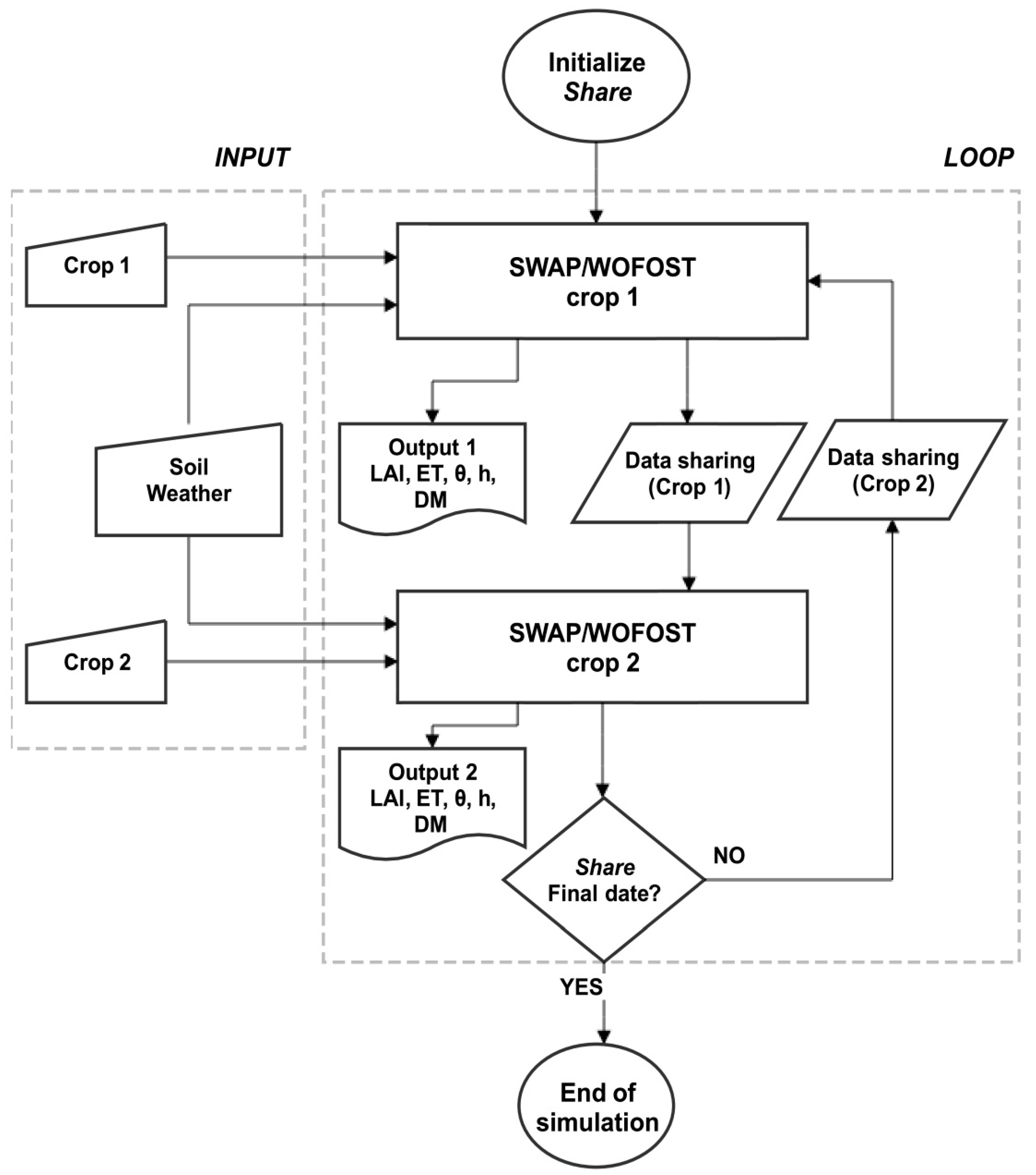
2.1.1. SWAP 2×1D
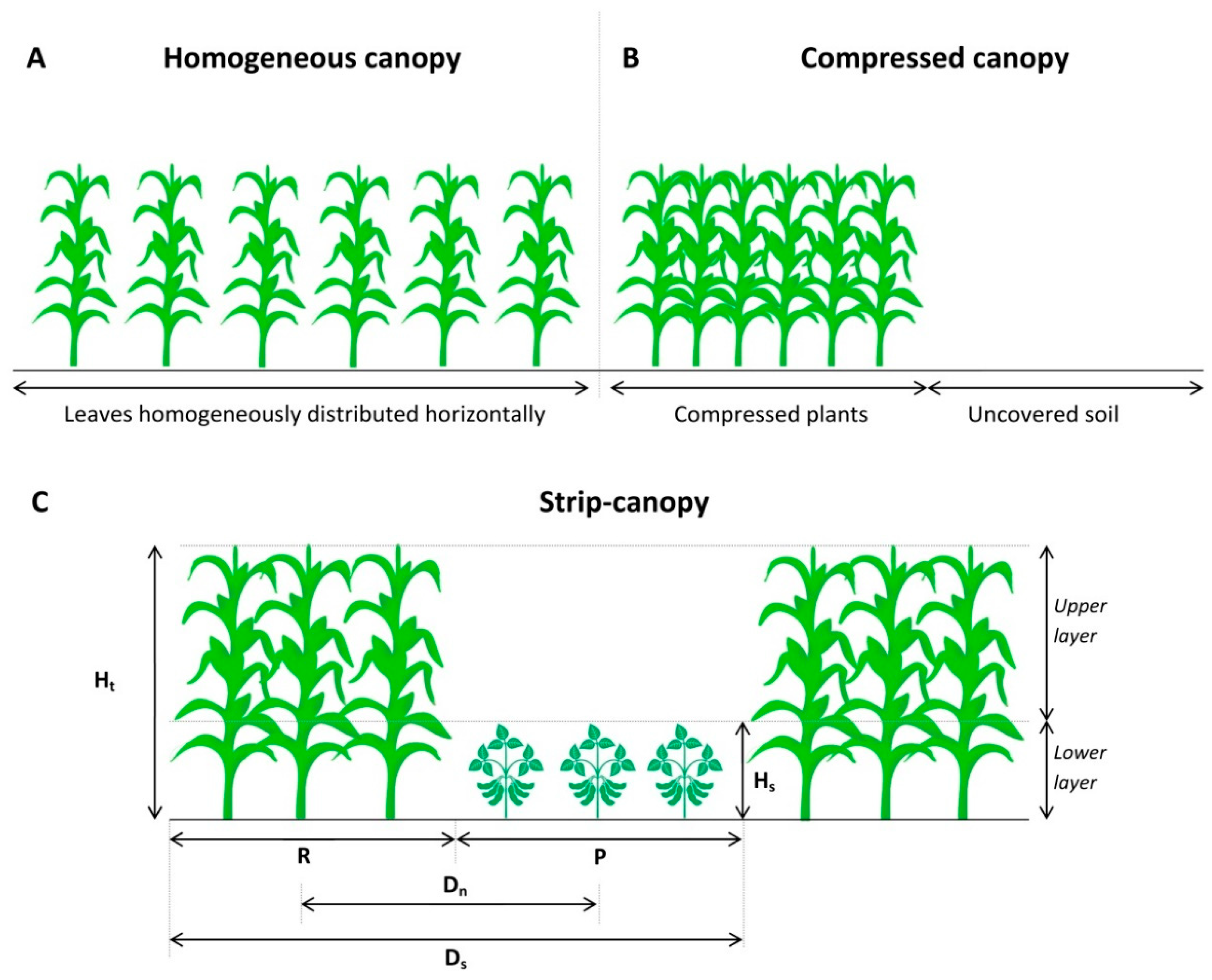
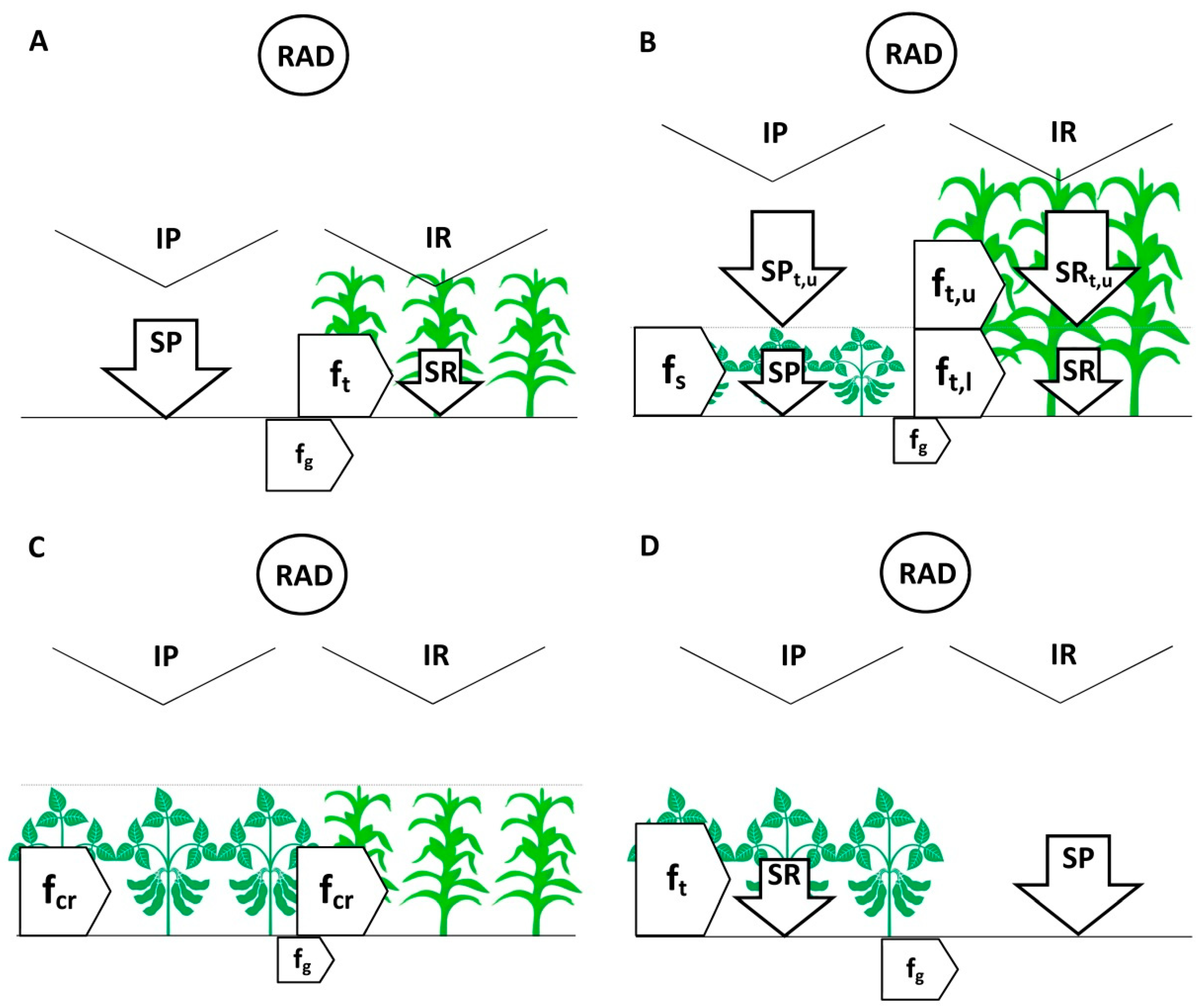
2.1.2. Radiation Interception
2.1.3. Atmospheric Vapor Fluxes
2.1.4. Lateral Soil Water Flux
2.1.5. Water Balance
2.2. Model Evaluation
2.3. Sensitivity Analysis
3. Results and Discussion
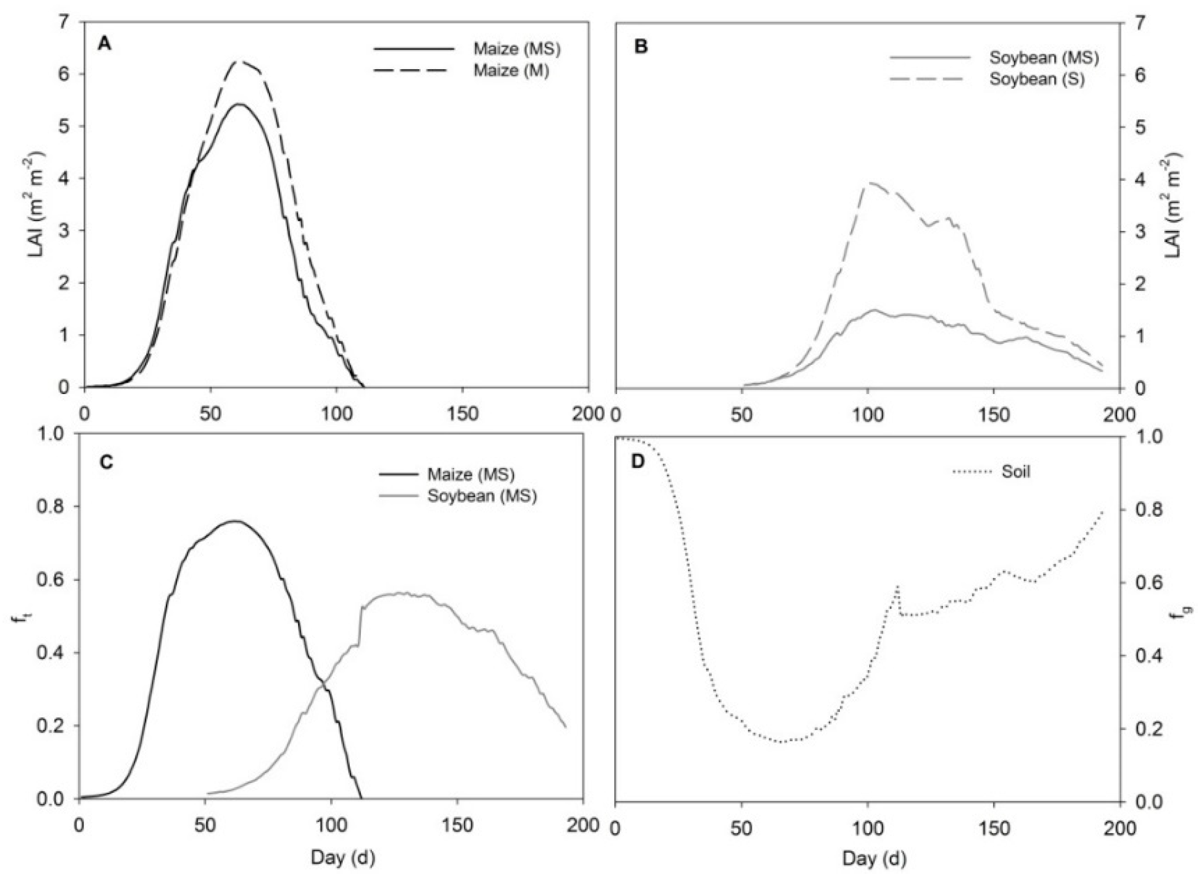
3.1. LAI and Radiation Interception
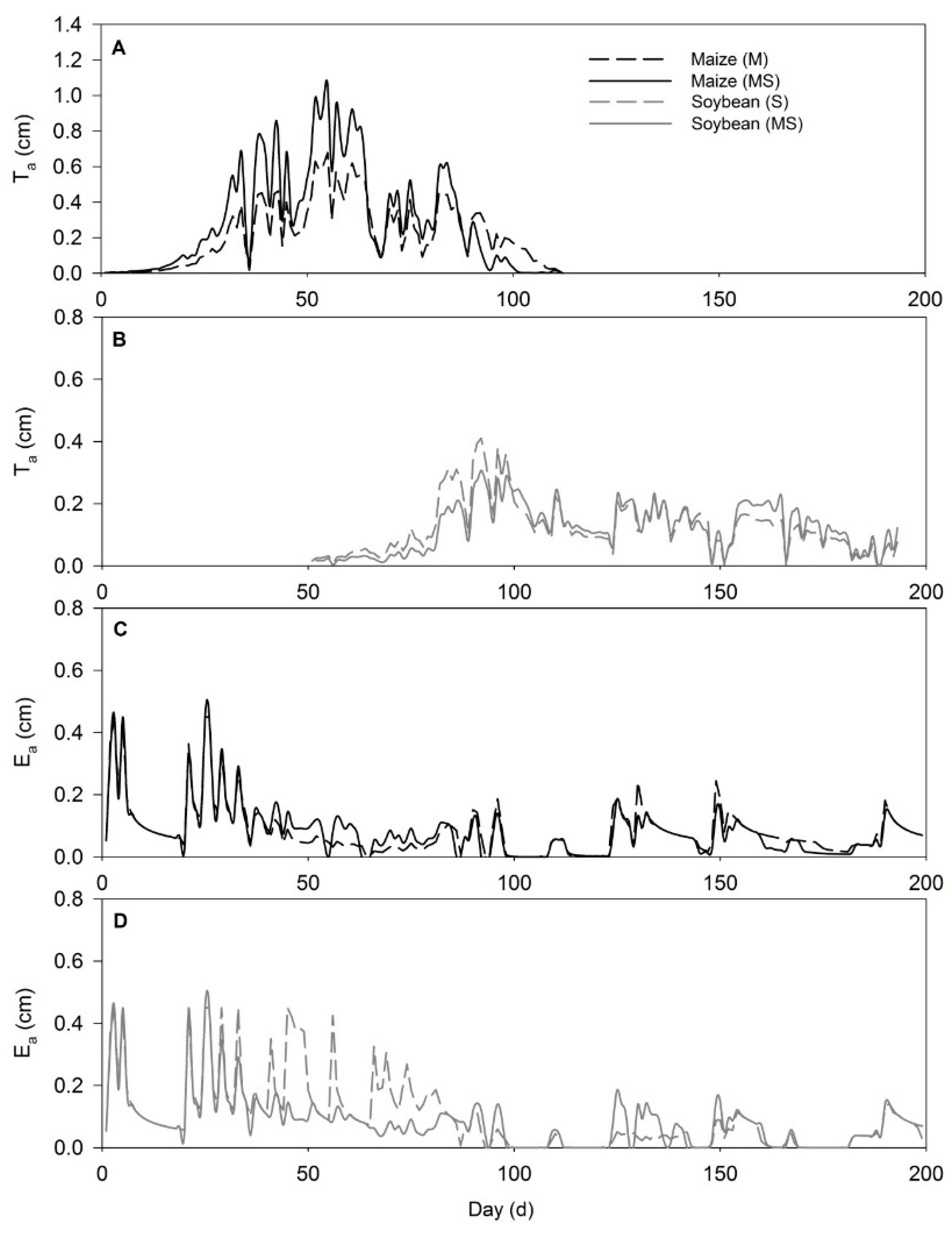
3.2. Transpiration and Evaporation Fluxes
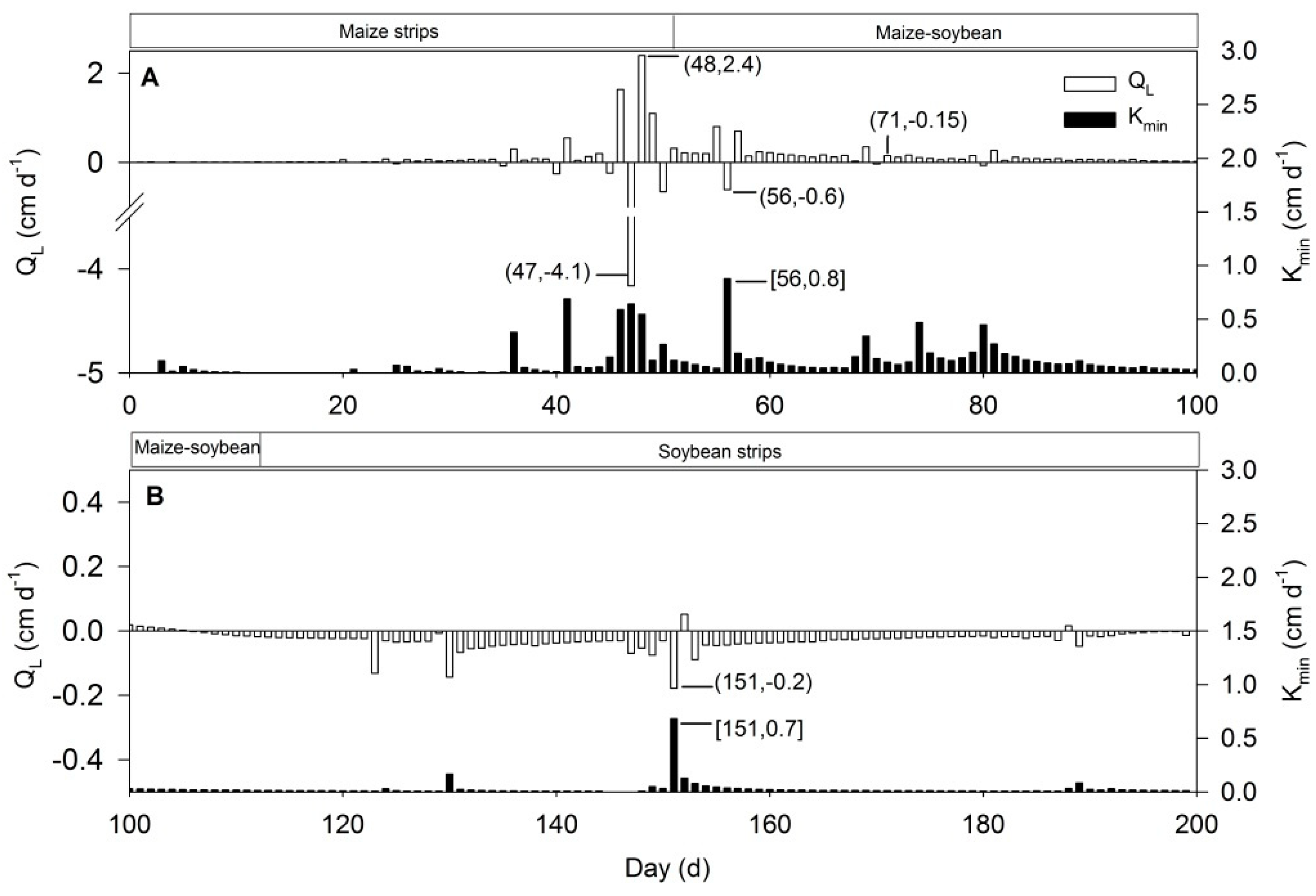
3.3. Lateral Soil Water Flux
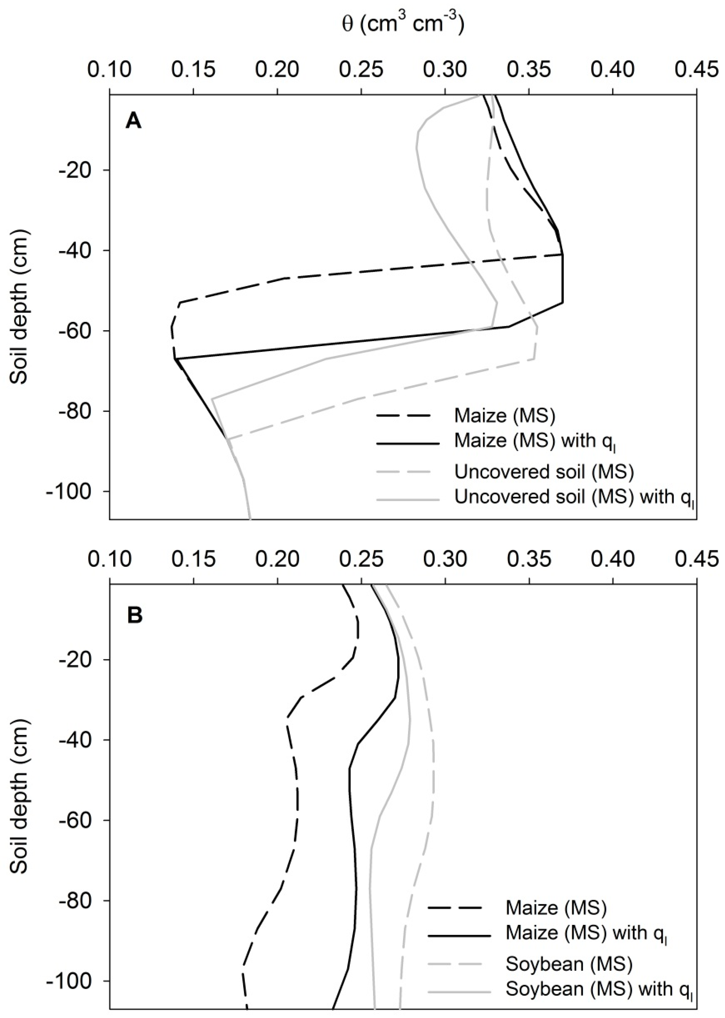
3.4. Water Balance
3.5. Sensitivity Analysis
4. Conclusions
Author Contributions
Funding
Acknowledgments
Conflicts of Interest
References
- Martin-Guay, M.-O.; Paquette, A.; Dupras, J.; Rivest, D. The new Green Revolution: Sustainable intensification of agriculture by intercropping. Sci. Total Environ. 2018, 615, 767–772. [Google Scholar] [CrossRef] [PubMed]
- Himmelstein, J.; Ares, A.; Gallagher, D.; Myers, J. A meta-analysis of intercropping in Africa: Impacts on crop yield, farmer income, and integrated pest management effects. Int. J. Agric. Sustain. 2017, 15, 1–10. [Google Scholar] [CrossRef]
- Temesgen, A.; Fukai, S.; Rodriguez, D. As the level of crop productivity increases: Is there a role for intercropping in smallholder agriculture. Field Crops Res. 2015, 180, 155–166. [Google Scholar] [CrossRef]
- Duchene, O.; Vian, J.-F.; Celette, F. Intercropping with legume for agroecological cropping systems: Complementarity and facilitation processes and the importance of soil microorganisms: A review. Agric. Ecosyst. Environ. 2017, 240, 148–161. [Google Scholar] [CrossRef]
- Wu, K.; Wu, B. Potential environmental benefits of intercropping annual with leguminous perennial crops in Chinese agriculture. Agric. Ecosyst. Environ. 2014, 188, 147–149. [Google Scholar] [CrossRef]
- Borghi, E.; Crusciol, C.A.C.; Nascente, A.S.; Mateus, G.P.; Martins, P.O.; Costa, C. Effects of row spacing and intercrop on maize grain yield and forage production of palisade grass. Crops Past. Sci. 2013, 63, 1106–1113. [Google Scholar] [CrossRef]
- Chauhan, B.S.; Singh, R.G.; Mahajan, G. Ecology and management of weeds under conservation agriculture: A review. Crops Prot. 2012, 38, 57–65. [Google Scholar] [CrossRef]
- Lithourgidis, A.S.; Dordas, C.A.; Damalas, C.A.; Vlachostergios, D.N. Annual intercrops: An alternative pathway for sustainable agriculture. Aus. J. Crops Sci. 2011, 5, 396–410. [Google Scholar]
- Bedoussac, L.; Journet, E.-P.; Hauggaard-Nielsen, H.; Naudin, C.; Corre-Hellou, G.; Jensen, E.S.; Prieur, L.; Justes, E. Ecological principles underlying the increase of productivity achieved by cereal-grain legume intercrops in organic farming. A review. Agron. Sustain. Dev. 2015, 35, 911–935. [Google Scholar] [CrossRef]
- Gaudio, N.; Escobar-Gutiérrez, A.J.; Casadebaig, P.; Evers, J.B.; Gérard, F.; Louarn, G.; Colbach, N.; Munz, S.; Launay, M.; Marrou, H.; et al. Current knowledge and future research opportunities for modeling annual crop mixtures. A review. Agron. Sustain. Dev. 2019, 39, 1–20. [Google Scholar] [CrossRef]
- Gou, F.; van Ittersum, M.K.; van der Werf, W. Simulating potential growth in a relay-strip intercropping system: Model description, calibration and testing. Field Crops Res. 2017, 200, 122–142. [Google Scholar] [CrossRef]
- Gou, F.; van Ittersum, M.K.; Simon, E.; Leffelaar, P.A.; van der Putten, P.E.L.; Zhang, L.Z.; van der Werf, W. Intercropping wheat and maize increases total radiation interception and wheat RUE but lowers maize RUE. Eur. J. Agron. 2017, 84, 125–139. [Google Scholar] [CrossRef]
- Wang, Z.; Zhao, X.; Wu, P.; He, J.; Chen, X.; Gao, Y.; Cao, X. Radiation interception and utilization by wheat/maize strip intercropping systems. Agric. Forest Meteorol. 2015, 204, 58–66. [Google Scholar] [CrossRef]
- Knörzer, H.; Graeff-Hönninger, S.; Müller, B.U.; Piepho, H.-P.; Claupein, W. A modeling approach to simulate effects of intercropping and interspecific competition in arable crops. Int. J. Inf. Syst. Soc. Chang. 2010, 1, 44–65. [Google Scholar] [CrossRef]
- Pronk, A.A.; Goudriaan, J.; Stilma, E.; Challa, H. A simple method to estimate radiation interception by nursery stock conifers: A case study of eastern white cedar. NJAS-Wagening J. Life Sci. 2003, 51, 279–295. [Google Scholar] [CrossRef]
- Baumann, D.T.; Bastiaans, L.; Goudriaan, J.; Van Laar, H.H.; Kropff, M.J. Analysing crop yield and plant quality in an intercropping system using an eco-physiological model for interplant competition. Agric. Syst. 2002, 73, 173–203. [Google Scholar] [CrossRef]
- Baumann, D.T.; Bastiaans, L.; Kropff, M.J. Intercropping system optimization for yield, quality, and weed suppression combining mechanistic and descriptive models. Agron. J. 2002, 94, 734–742. [Google Scholar] [CrossRef]
- Chimonyo, V.G.P.; Modi, A.T.; Mabhaudhi, T. Perspective on crop modeling in the management of intercropping systems. Arch. Agron. Soil Sci. 2015, 61, 1511–1529. [Google Scholar] [CrossRef]
- Ozier-Lafontaine, H.; Lafolie, F.; Bruckler, L.; Tournebize, R.; Mollier, A. Modelling competition for water in intercrops: Theory and comparison with field experiments. Plant Soil 1998, 204, 183–201. [Google Scholar] [CrossRef]
- Berntsen, J.; Hauggard-Nielsen, H.; Olesen, J.E.; Petersen, B.M.; Jensen, E.S.; Thomsen, A. Modelling dry matter production and resource use in intercrops of pea and barley. Field Crops Res. 2004, 88, 69–83. [Google Scholar] [CrossRef]
- O’Callaghan, J.R.; Maende, C.; Wyseure, G.C.L. Modelling the intercropping of maize and beans in Kenya. Comput. Electron. Agric. 1994, 11, 351–365. [Google Scholar] [CrossRef]
- Chen, H.; Qin, A.; Chai, Q.; Gan, Y.; Liu, Z. Quantification of soil water competition and compensation using soil water differences between strips of intercropping. Agric. Res. 2014, 3, 321–330. [Google Scholar] [CrossRef]
- Karray, J.A.; Lhomme, J.P.; Masmoudi, M.M.; Mechlia, N.B. Water balance of the olive tree–annual crop association: A modeling approach. Agric. Water Manag. 2008, 95, 575–586. [Google Scholar] [CrossRef]
- Kroes, J.G.; Van Dam, J.C.; Bartholomeus, R.P.; Groenendijk, P.; Heinen, M.; Hendriks, R.F.A.; Mulder, H.M.; Supit, I.; Van Walsum, P.E.V. SWAP Version 4.0. Theory Description and User Manual; Alterra: Wageningen, The Netherlands, 2017. [Google Scholar]
- van Diepen, C.A.; Wolf, J.; van Keulen, C.; Rappoldt, C. WOFOST: A simulation model of crop production. Soil Use Manag. 1989, 5, 16–24. [Google Scholar] [CrossRef]
- Goudriaan, J. Crop Micrometeorology: A Simulation Study (Simulation Monographs); Pudoc, Center for Agricultural Publishing and Documentation: Wageningen, The Netherlands, 1977. [Google Scholar]
- Monteith, J.L. Evaporation and Surface Temperature, Quart. J. R. Meteorol. Soc. 1981, 107, 1–24. [Google Scholar] [CrossRef]
- Wallace, J.S. Evaporation and radiation interception by neighbouring plants. Q. J. R. Meteorol. Soc. 1997, 123, 1885–1905. [Google Scholar] [CrossRef]
- Gao, Y.; Duan, A.; Qiu, X.; Liu, Z.; Sun, J.; Zhang, J.; Wang, H. Distribution of roots and root length density in a maize/soybean strip intercropping system. Agric. Water Manag. 2010, 98, 199–212. [Google Scholar] [CrossRef]
- Gao, Y.; Duan, A.; Qiu, X.; Li, X.; Pauline, U.; Sun, J.; Wang, H. Modeling evapotrasnpiration in maize/soybean strip intercropping system with the evaporation and radiation interception by neighboring species model. Agric. Water Manag. 2013, 128, 110–119. [Google Scholar] [CrossRef]
- Miao, Q.; Rosa, R.D.; Shi, H.; Paredes, P.; Zhu, L.; Dai, J.; Gonçalves, J.M.; Pereira, L.S. Modeling water use, transpiration and soil evaporation of spring wheat–maize and spring wheat–sunflower relay intercropping using the dual crop coefficient approach. Agric. Water Manag. 2016, 165, 211–229. [Google Scholar] [CrossRef]
- De Jong van Lier, Q. Field capacity, a valid upper limit of crop available water? Agric. Water Manag. 2017, 193, 214–220. [Google Scholar] [CrossRef]
- Feddes, R.A.; Kowalik, P.J.; Zaradny, J. Simulation of Field Water Use and Crops Yield; Simulation Monographs; PUDOC: Wageningen, The Netherlands, 1978; p. 189. [Google Scholar] [CrossRef]
- Liu, X.; Rahman, T.; Yang, F.; Song, C.; Yong, T.; Liu, J.; Zhang, C.; Yang, W. PAR interception and utilization in different maize and soybean intercropping patterns. PLoS ONE 2017, 12, 1–17. [Google Scholar] [CrossRef] [PubMed]


| Symbol | Description | Equation | Unit |
|---|---|---|---|
| Radiation | |||
| ft | Fraction of radiation intercepted by a strip-canopy | (1) | - |
| fh | Fraction of radiation intercepted by a homogeneous type canopy | (2) | - |
| fc | Fraction of radiation intercepted by a compressed type canopy | (3) | |
| LAI | Leaf area index over the whole intercropped area | - | m2 m−2 |
| LAIc | Leaf area index of a compressed canopy | (4) | m2 m−2 |
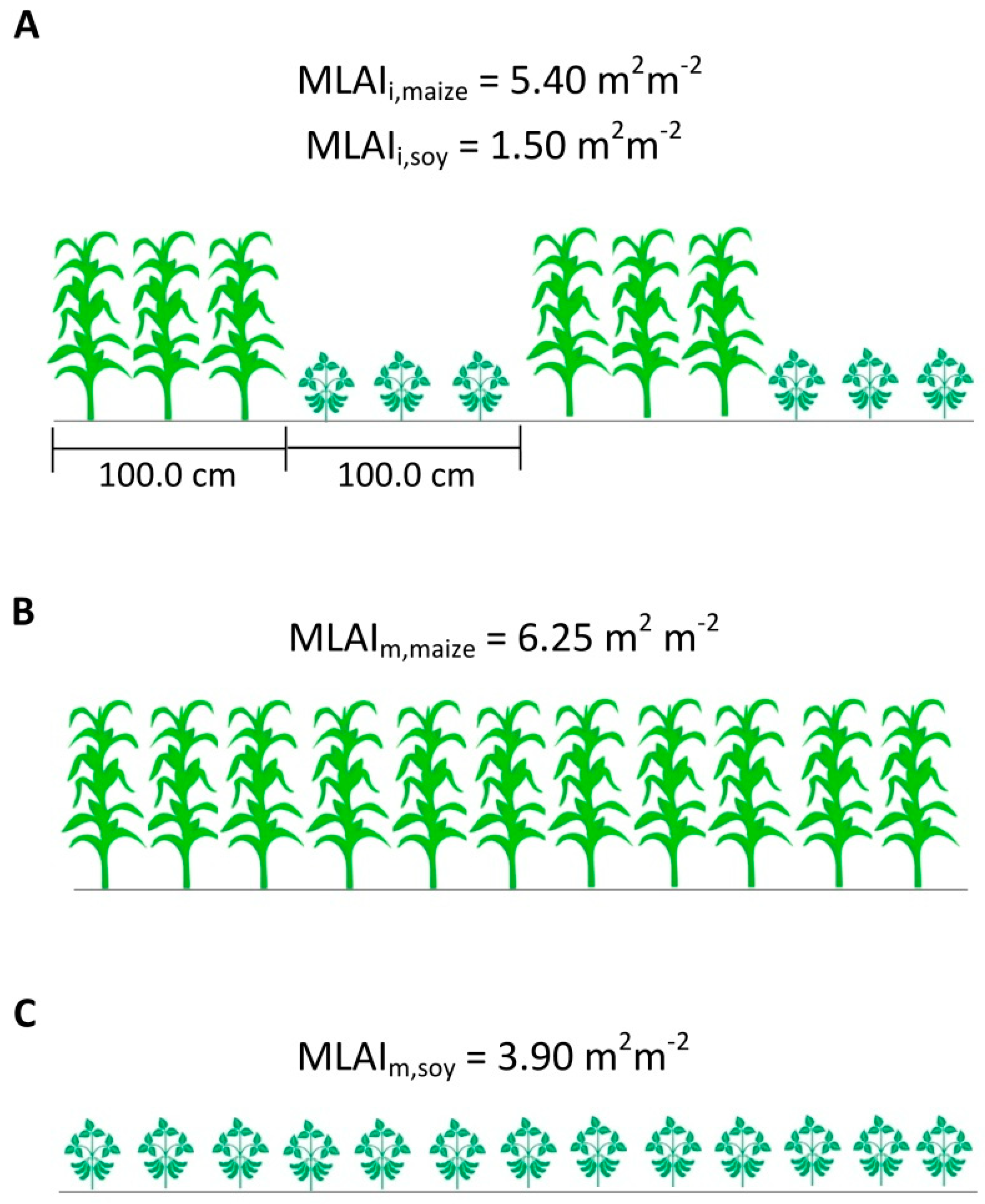
| MLAIi | Maximum leaf area index over the whole intercropped area | m2 m−2 | |
| MLAIm | Maximum leaf area index over the whole monocropping area | m2 m−2 | |
| w | Factor expressing the relative homogeneous and compressed contribution to the canopy radiation interception model | (5) | - |
| SR | Fraction of radiation reaching the soil under the strip | (6) | - |
| SP | Fraction of radiation reaching the soil path | (7) | - |
| IP | View factor over the soil path | (8) | - |
| IR | View factor over the strip | (9) | - |
| LAIt,u | Leaf area index of the taller plants in the upper canopy layer | (10) | m2 m−2 |
| LAIt,l | Leaf area index of the taller plants in the lower canopy layer | (11) | m2 m−2 |
| LAIs,c | Leaf area index compressed of the shorter plant | ||
| ft,l | Fraction of radiation interception by the taller plant in the lower layer | (13) | - |
| ft,u | Fraction of radiation interception by the taller plant in the upper layer | (1)–(9) | - |
| SRt,u | Fraction of radiation transmitted through the upper part of the taller plants | (14) | - |
| fs | Fraction of radiation intercepted by the shorter plants | (15) | - |
| SPt,u | Fraction of radiation transmitted between and through the taller plant to the path | (16) | - |
| fcr | Fraction of radiation intercepted by strip plants with the same height | (17) | - |
| fg | Fraction of radiation intercepted by the soil | (18) | - |
| ft1 | Total fraction of the radiation interception by one plant species in the intercropping | (18) | - |
| ft2 | Total fraction of the radiation interception by a second plant species in the intercropping | (18) | - |
| kcf | Light extinction coefficient | - | - |
| ks | Light extinction coefficient of the shorter plant | - | - |
| kt | Light extinction coefficient of the shorter plant | - | - |
| kcr | Light extinction coefficient of a intercropped plant | - | - |
| R | Strip width | - | cm |
| P | Path width | - | cm |
| Ht | Plant height of the taller plant in the intercrop | - | cm |
| Hs | Plant height of the shorter plant in the intercrop | - | cm |
| Rt | Strip width of the taller plant in the intercrop | - | cm |
| Pt | Path width of the taller plant in the intercrop | - | cm |
| Rs | Strip width of the shorter plant in the intercrop | - | cm |
| Ps | Path width of the shorter plant in the intercrop | - | cm |
| Rcr | Strip width of a intercropped plant | - | cm |
| Pcr | Path width of a intercropped plant | - | cm |
| Water flux | |||
| Tp,i | Potential transpiration of each plant separately | (19) | cm |
| Ep | Potential evaporation | (20) | cm |
| Wc | Fraction of the day during which the canopy is wet | (19) | - |
| ∆v | Slope of the saturated vapor pressure-temperature curve | (19), (20) | kPa °C−1 |
| λw | Latent heat of vaporization | (19), (20) | kJ kg−1 |
| Rn | Net radiation at the canopy surface | (19), (20) | J m−2 d−1 |
| G | Soil heat flux density | (19), (20) | J m−2 d−1 |
| p1 | Unit conversion value | (19), (20) | s d−1 |
| ρa | Air density | (19), (20) | kg m−3 |
| Ca | Heat capacity of the moist air | (19), (20) | J kg−1 °C−1 |
| esat | Saturation vapor pressure | (19), (20) | kPa |
| ea | Actual vapor pressure | (19), (20) | kPa |
| γa | Psychrometric constant | (19), (20) | kPa °C−1 |
| ra,c,i | Aerodynamic resistance of the plant canopy | (21) | s m−1 |
| ra,g | Aerodynamic resistance of the soil | (22) | s m−1 |
| rs,min,i | Minimum stomatal resistance | (19) | s m−1 |
| LAIeff | Effective leaf area index | (19) | |
| rsoil | Soil resistance of a wet soil | (20) | s m−1 |
| Pin,i | Water interception by the plant canopy | (23) | cm |
| Pgross | Gross precipitation | (23) | cm d−1 |
| a | Empirical coefficient for the precipitation interception | (23) | |
| ql,d | Lateral Darcian water flux between soil compartments | (24) | cm d−1 |
| Kmin | Hydraulic conductivity of the driest same-level soil compartment | (24) | cm d−1 |
| Dn | Distance between the centers of two neighboring strips of different plant species | (24), (25) | cm |
| h1, h2 | Soil pressure head | (24) | cm |
| qlim,d | Limiting lateral flux per compartment | (25) | cm d−1 |
| ∆θ | Difference in soil water content of two same-level soil compartments | (25) | |
| qd | Lateral flux per soil compartment limited by qlim | (26) | cm d−1 |
| Bc,i | Plant-ground coverage fraction | (27), (31) | cm2 cm−2 |
| QL | Total lateral flux of the soil profile | (27) | cm d−1 |
| Water balance | |||
| Pa | Precipitation | (29), (30) | cm |
| Ta | Plant transpiration | (29), (30) | cm |
| Ea | Soil evaporation | (29), (30) | cm |
| Qb | Bottom flux | (29), (30) | cm |
| ∆S1 | Variation of soil water storage in soil-plant module 1 | (29), (31) | cm |
| ∆S2 | Variation of soil water storage in soil-plant module 2 | (30), (31) | cm |
| ∆Sin | Variation of soil water storage for the intercropping | (30), (31) | cm |
| Sensitivity analysis | |||
| η | Relative partial sensitivity index | (32) | - |
| Vf | Default value of a generic output variable | (32) | |
| Vs | New value of the output variable after a selected parameter was changed | (32) | |
| Vr | Reference value of the output variables evaluated in the sensitivity analysis | (32) | |
| p | General representation for parameter | (32) | |
| ∆p | Change in the parameter values in the sensitivity analysis | (32) | |
| Cref | Canopy reflection coefficient | - | |
| RLAI | Maximum relative increase in LAI | m2 m−2 d−1 | |
| kdif | Extinction coefficient for diffuse light | - | |
| kdir | Extinction coefficient for direct light | - | |
| Өr | Saturated soil water content | cm3 cm−3 | |
| Өs | Residual soil water content | cm3 cm−3 | |
| α | Soil water retention curve parameter | cm−1 | |
| n | Soil water retention curve parameter | - | |
| Ks | Saturated hydraulic conductivity | cm d−1 | |
| l | Soil hydraulic conductivity exponent | - |
| Scenario | Model | Description | Objective |
|---|---|---|---|
| Maize–soybean (MS) intercropping | SWAP 2×1D | Strip intercropping MS (Figure 4A). Soybean is sown approximately 50 days after maize. | Application of SWAP 2×1D to a strip intercropping system |
| Maize monocropping (M) | SWAP 1D | Monocropping cultivation of maize (Figure 4B) | To compare the water balance outcomes of monocropping to the intercropping scenario. |
| soybean monocropping (B) | SWAP 1D | Monocropping cultivation of soybean (Figure 4C) | To compare the water balance outcomes of monocropping to the intercropping scenario. |
| Description | Parameter | Maize | Soybean | Unit |
|---|---|---|---|---|
| Plant maximum height | Hmax | 200 | 80 | cm |
| Reflection coefficient, Albedo | Cref | 0.20 | 0.23 | - |
| Minimum canopy resistance | RSC | 131 | 70 | s m−1 |
| Temperature sum from emergence to anthesis | Tsum,ea | 1000 | - | °C |
| Temperature sum from anthesis to maturity | Tsum,am | 1150 | - | °C |
| Maximum CO2 assimilation rate | Amax,d | 35 | 37 | kg ha−1 d−1 |
| Maximum relative increase in LAI | RLAI | 0.012 | 0.010 | m2 m2 |
| Extinction coefficient for diffuse visible light | kdif | 0.60 | 0.80 | - |
| Extinction coefficient for direct visible light | kdir | 0.75 | 0.80 | - |
| Light use efficiency | eff | 0.45 | 0.40 | kg CO2 J−1 |
| Assimilates conversion efficiency into leaves | Cvl | 0.68 | 0.72 | kg kg−1 |
| Assimilates conversion efficiency into storage organs | Cvo | 0.67 | 0.68 | kg kg−1 |
| Assimilates conversion efficiency into roots | Cvr | 0.29 | 0.72 | kg kg−1 |
| Assimilates conversion efficiency into stems | Cvs | 0.66 | 0.69 | kg kg−1 |
| Relative increase in respiration rate with temperature | Rit | 2.00 | 2.00 | kg CH2O kg−1 d−1 |
| Relative maintenance respiration rate of leaves | Rml | 0.03 | 0.03 | kg CH2O kg−1 d−1 |
| Relative maintenance respiration rate of storage organs | Rmo | 0.01 | 0.017 | kg CH2O kg−1 d−1 |
| Relative maintenance respiration rate of roots | Rmr | 0.015 | 0.010 | kg CH2O kg−1 d−1 |
| Relative maintenance respiration rate of stems | Rms | 0.015 | 0.015 | kg CH2O kg−1 d−1 |
| Maximum relative death rate of leaves due to water stress | Pdl | 0.03 | 0.03 | d−1 |
| Critical pressure heads according to Feddes [33] | h1 | −10.0 | −15.0 | cm |
| h2u | −25.0 | −30.0 | cm | |
| h2l | −25.0 | −30.0 | cm | |
| h3h | −400.0 | −750.0 | cm | |
| h3l | −500.0 | −2000.0 | cm | |
| h4 | −10000.0 | −8000.0 | cm | |
| Interception coefficient, corresponding to maximum interception amount | a | 0.25 | 0.25 | cm |
| Maximum daily increase in rooting depth | Rrd,i | 2.20 | 1.2 | cm d−1 |
| Maximum root depth | Rd,m | 100 | 100 | cm |
| Below ground plant coverage | Bc | 0.5 | 0.5 | - |
| Description | Parameter | Value | Unit |
|---|---|---|---|
| Soil resistance of wet soil | rsoil | 230 | s m−1 |
| Soil evaporation coefficient of Black | Cbk | 0.45 | cm1/2 |
| Residual water content | Өr | 0.13 | cm3 cm−3 |
| Saturated water content | Өs | 0.37 | cm3 cm−3 |
| Parameter alfa of the water retention curve | α | 0.04 | cm−1 |
| Parameter n of the water retention curve | n | 1.59 | - |
| Exponent in the hydraulic conductivity function | l | 1.2 | - |
| Hydraulic conductivity at saturated conditions | Ksat | 26 | cm d−1 |
| Water Balance Components | SWAP 1D | SWAP 2×1D | ||
|---|---|---|---|---|
| (cm) | Maize | Soybean | MS 1D Average | MS |
| Actual | ||||
| ∆S | 4.1 | 1.1 | 2.6 | 1.1 |
| Pa | 47.7 | 47.7 | 47.7 | 47.7 |
| Pi | −2.7 | −1.0 | −1.9 | −1.6 |
| ETa | −40.8 | −37.2 | −39.0 | −41.6 |
| Ta | −24.6 | −17.7 | −21.1 | −25.4 |
| Ea | −16.2 | −19.5 | −17.9 | −16.1 |
| Qb | −0.1 | −8.3 | −4.2 | −3.5 |
| Potential | ||||
| ETp | 74.3 | 75.0 | 74.7 | 73.2 |
| Tp | 24.6 | 24.2 | 24.4 | 31.4 |
| Ep | 49.7 | 50.8 | 50.3 | 41.8 |
| Parameter | η | |||||||||||||
|---|---|---|---|---|---|---|---|---|---|---|---|---|---|---|
| Maize | Soybean | |||||||||||||
| ∑ft | Tp | Ta | Ep | Ea | QL | Qb | ∑ft | Tp | Ta | Ep | Ea | QL | Qb | |
| Maize | ||||||||||||||
| RUE | 0.17 | 0.63 | −0.11 | 0.00 | −0.21 | −0.21 | −0.42 | 0.00 | 0.00 | 0.00 | −0.42 | −0.11 | 0.21 | 0.00 |
| Cref | 0.01 | −1.16 | 1.05 | 0.00 | 0.00 | 1.05 | 2.21 | −0.01 | 0.00 | 0.00 | 0.00 | 0.00 | −1.05 | −1.16 |
| RLAI | 0.27 | 1.26 | −2.00 | −0.01 | −0.42 | −2.31 | −4.62 | −0.01 | 0.00 | 0.11 | −0.74 | −0.21 | 2.31 | 2.00 |
| kdif | 0.19 | 0.53 | 0.00 | 0.00 | −0.42 | −0.42 | −0.95 | −0.07 | −0.21 | 0.11 | −0.42 | −0.11 | 0.42 | 0.21 |
| kdir | 0.40 | 1.26 | 0.42 | −0.01 | −0.53 | −0.11 | −0.11 | −0.06 | −0.21 | 0.11 | −0.84 | −0.21 | 0.11 | −0.32 |
| Soil | ||||||||||||||
| Өr | 0.00 | 0.00 | 0.32 | 0.00 | 0.11 | 0.74 | 1.47 | −0.18 | −0.42 | 0.63 | 0.21 | −0.11 | −0.74 | −1.58 |
| Өs | 0.01 | 0.00 | 5.78 | 0.00 | 1.26 | 7.04 | 14.18 | 0.09 | −0.32 | 0.53 | 0.11 | 1.05 | −7.04 | −7.25 |
| a | −0.03 | −0.11 | −1.16 | 0.00 | 0.00 | −0.74 | −1.47 | −0.12 | −0.32 | 0.42 | 0.21 | 0.00 | 0.74 | 0.53 |
| n | 0.00 | 0.00 | −1.37 | 0.00 | −0.42 | −0.53 | −1.16 | −0.16 | −0.32 | 0.63 | 0.21 | −0.21 | 0.53 | −0.21 |
| Ks | 0.00 | 0.00 | 1.47 | 0.00 | 0.11 | 1.79 | 3.68 | 0.01 | 0.00 | 0.00 | −0.11 | 0.00 | −1.79 | −2.31 |
| l | 0.00 | −0.11 | −0.21 | 0.00 | −0.11 | −0.21 | −0.42 | 0.02 | 0.00 | 0.00 | 0.00 | 0.00 | 0.21 | 0.32 |
© 2019 by the authors. Licensee MDPI, Basel, Switzerland. This article is an open access article distributed under the terms and conditions of the Creative Commons Attribution (CC BY) license (http://creativecommons.org/licenses/by/4.0/).
Share and Cite
Pinto, V.M.; van Dam, J.C.; de Jong van Lier, Q.; Reichardt, K. Intercropping Simulation Using the SWAP Model: Development of a 2×1D Algorithm. Agriculture 2019, 9, 126. https://doi.org/10.3390/agriculture9060126
Pinto VM, van Dam JC, de Jong van Lier Q, Reichardt K. Intercropping Simulation Using the SWAP Model: Development of a 2×1D Algorithm. Agriculture. 2019; 9(6):126. https://doi.org/10.3390/agriculture9060126
Chicago/Turabian StylePinto, Victor Meriguetti, Jos C. van Dam, Quirijn de Jong van Lier, and Klaus Reichardt. 2019. "Intercropping Simulation Using the SWAP Model: Development of a 2×1D Algorithm" Agriculture 9, no. 6: 126. https://doi.org/10.3390/agriculture9060126
APA StylePinto, V. M., van Dam, J. C., de Jong van Lier, Q., & Reichardt, K. (2019). Intercropping Simulation Using the SWAP Model: Development of a 2×1D Algorithm. Agriculture, 9(6), 126. https://doi.org/10.3390/agriculture9060126