Multi-Temporal Point Cloud Alignment for Accurate Height Estimation of Field-Grown Leafy Vegetables

Abstract

Accurate measurement of plant height in leafy vegetables is challenging due to their short stature, high planting density, and severe canopy occlusion during later growth stages. These factors often limit the reliability of single-plant monitoring across the full growth cycle in open-field environments. To address this, we propose a multi-temporal point cloud alignment method for accurate plant height measurement, focusing on Choy Sum (Brassica rapa var. parachinensis). The method estimates plant height by calculating the vertical distance between the canopy and the ground. Multi-temporal point cloud maps are reconstructed using an enhanced Oriented FAST and Rotated BRIEF–Simultaneous Localization and Mapping (ORB-SLAM3) algorithm. A fixed checkerboard calibration board, leveled using a spirit level, ensures proper vertical alignment of the Z-axis and unifies coordinate systems across growth stages. Ground and plant points are separated using the Excess Green (ExG) index. During early growth stages, when the soil is minimally occluded, ground point clouds are extracted and used to construct a high-precision reference ground model through Cloth Simulation Filtering (CSF) and Kriging interpolation, compensating for canopy occlusion and noise. In later growth stages, plant point cloud data are spatially aligned with this reconstructed ground surface. Individual plants are identified using an improved Euclidean clustering algorithm, and consistent measurement regions are defined. Within each region, a ground plane is fitted using the Random Sample Consensus (RANSAC) algorithm to ensure alignment with the X–Y plane. Plant height is then determined by the elevation difference between the canopy and the interpolated ground surface. Experimental results show mean absolute errors (MAEs) of 7.19 mm and 18.45 mm for early and late growth stages, respectively, with coefficients of determination (R²) exceeding 0.85. These findings demonstrate that the proposed method provides reliable and continuous plant height monitoring across the full growth cycle, offering a robust solution for high-throughput phenotyping of leafy vegetables in field environments.

1. Introduction

Plant height is a key phenotypic trait for assessing plant physiological status and growth dynamics and is commonly defined as the perpendicular distance from the root collar to the highest photosynthetically active tissue within the canopy [1,2]. In agronomic research and crop phenotyping, plant height is typically estimated as the elevation difference between the canopy surface and the ground [3]. However, manual measurement is labor-intensive, invasive, and prone to sampling bias due to limited sample sizes, which constrains its applicability for large-scale and long-term field monitoring [4]. With the development of high-throughput, non-destructive sensing technologies, image- and point cloud–based methods have increasingly replaced manual measurements. Two-dimensional (2D) image-based approaches are attractive due to their low cost and simplicity but are inherently limited by the absence of three-dimensional (3D) structural information, resulting in reduced robustness under complex field conditions [5,6,7]. In contrast, three-dimensional sensing technologies—such as stereovision, depth cameras, and Light Detection and Ranging (LiDAR)—enable automated plant height estimation through point cloud analysis and provide additional spatial information related to canopy structure and geometry [8].

Stereovision-based methods reconstruct three-dimensional crop structures via multi-view image matching and have been widely applied in unmanned aerial vehicle (UAV) platforms and ground-based phenotyping systems due to their flexibility and relatively low cost [9,10,11]. Recent studies have further combined stereovision with Simultaneous Localization and Mapping (SLAM) techniques to support multi-temporal field reconstruction [12,13,14]. For example, Dong et al. [12] proposed a four-dimensional reconstruction framework that integrates multi-sensor SLAM with Real-Time Kinematic Global Positioning System (RTK-GPS), enabling the unified registration of point clouds acquired from a peanut field at different growth stages and the estimation of plant height over time. However, this method relies primarily on feature-based stereo vision, which remains sensitive to illumination variations and appearance degradation in agricultural environments characterized by dense canopies, near-ground regions, or highly repetitive textures. Moreover, the consistent alignment of multi-temporal point clouds depends heavily on high-precision RTK-GPS priors, while at the crop scale, pose estimation errors in visual–inertial SLAM may still accumulate over time, adversely affecting reconstruction accuracy in later stages. These limitations further reduce the applicability of such approaches to short-stature crops or scenarios with severe occlusion during advanced growth stages.

Laser-based sensing technologies, including terrestrial laser scanners and LiDAR systems, can acquire high-precision three-dimensional point cloud data and have been widely applied to plant height estimation on ground-based platforms and UAVs. High measurement accuracy has been reported under relatively sparse canopy conditions. For instance, Sun et al. [15] achieved a coefficient of determination (R²) of 0.934 and a root mean square error (RMSE) of 3.51 mm when measuring rapeseed height using a mobile LiDAR system, while Obanawa et al. [13] demonstrated that handheld LiDAR outperformed Structure-from-Motion (SfM) approaches in grassland height estimation. Despite these advantages, LiDAR-based methods are constrained by high equipment costs, substantial computational requirements, and reduced data reliability under dense canopies due to occlusion and multiple laser returns. In addition, the lack of color information in most LiDAR datasets limits their applicability for continuous, individual-plant height monitoring throughout the full growth cycle [13,16,17].

RGB–Depth (RGB-D) cameras, which simultaneously acquire color and depth information, have emerged as a promising alternative for plant height estimation in both controlled and open-field environments [4,18]. Owing to their limited sensing range, these systems are primarily deployed on ground-based platforms [19]. Previous studies have demonstrated good performance at early growth stages. For example, Zhao et al. [20] achieved millimeter-level accuracy when estimating lettuce height under controlled conditions, while Qiu et al. [18] reported strong correlations between RGB-D–derived and manual measurements for maize at the jointing stage. However, field applications using RGB-D sensors often suffer from performance degradation under uneven terrain and complex soil backgrounds [21,22]. More importantly, most existing RGB-D–based approaches rely on independent frame-level measurements and lack a unified spatial reference for multi-temporal alignment. Consequently, cumulative spatial drift and inconsistent ground references limit their suitability for long-term field monitoring. Furthermore, these methods are typically restricted to seedling or early growth stages, when ground surfaces remain visible and canopy occlusion is minimal [23,24], making them inadequate for dense, late-stage field-grown leafy vegetables.

Overall, existing plant height measurement methods remain inadequate for field-grown leafy vegetables, particularly for continuous multi-temporal monitoring across the full growth cycle. Near-ground sensing approaches typically rely on persistent ground visibility and clear plant separation, assumptions that fail under dense planting and severe interleaf occlusion at later growth stages. Aerial and multi-view methods, on the other hand, often depend on static terrain references or implicit global coordinate alignment, making them vulnerable to spatial drift and ground reference inconsistencies caused by transplantation and early-stage soil disturbance. Consequently, robust multi-temporal point cloud alignment and consistent canopy-to-ground height estimation remain challenging for leafy vegetables characterized by short stature, prostrate growth habits, dense canopies, and rapidly diminishing ground visibility.

To address these challenges, this study takes Choy Sum (Brassica rapa var. parachinensis) as a representative leafy vegetable and proposes a multi-temporal point cloud alignment framework for plant height monitoring throughout the entire growth cycle. The framework establishes a unified world coordinate system using fixed reference constraints, enabling reliable alignment of point clouds acquired at different time points without reliance on GPS. A persistent ground reference model is reconstructed from early-stage ground observations and subsequently integrated with later-stage plant point clouds, effectively decoupling ground modeling from canopy measurement when the ground surface becomes occluded. Furthermore, geometric constraints and planting structure priors are incorporated to enhance the robustness of individual plant height estimation under dense planting and uneven terrain.

The main contributions of this study are summarized as follows:

• A multi-temporal point cloud alignment framework is proposed for short-stature, densely planted leafy vegetables under severe canopy occlusion, enabling reliable plant height monitoring throughout the entire growth cycle in open-field environments.
• A persistent reference ground modeling strategy is introduced by reconstructing the ground surface from early-stage point clouds and integrating it with later-stage plant data, effectively decoupling ground modeling from canopy measurement when ground visibility is lost.
• A unified and stable spatial reference is established using fixed calibration constraints in combination with local ground plane correction and planting structure priors, improving the robustness and accuracy of individual plant height estimation under uneven terrain and dense planting conditions.

2. Materials and Methods

2.1. Experimental Site and Data Acquisition

This study was conducted in November 2023 at the Qilin Farm of South China Agricultural University (113°22′38.95″ E, 23°10′9.31″ N). The experiment utilized Choy Sum (Brassica rapa var. parachinensis) plants, which were cultivated in deep furrows and high ridges with 15 cm spacing between plants. Data collection began on the 5th day after transplanting and was repeated every 48 h, spanning 11 time points from day 5 to day 25 to continuously monitor the growth of plant throughout its entire growth cycle. At each time point, RGB-D sequences were captured from approximately 200 plants, with each sequence comprising 1500–2000 frames of imagery along with corresponding Inertial Measurement Unit (IMU) data. The point cloud map covered an area of approximately 6 m × 1.5 m.

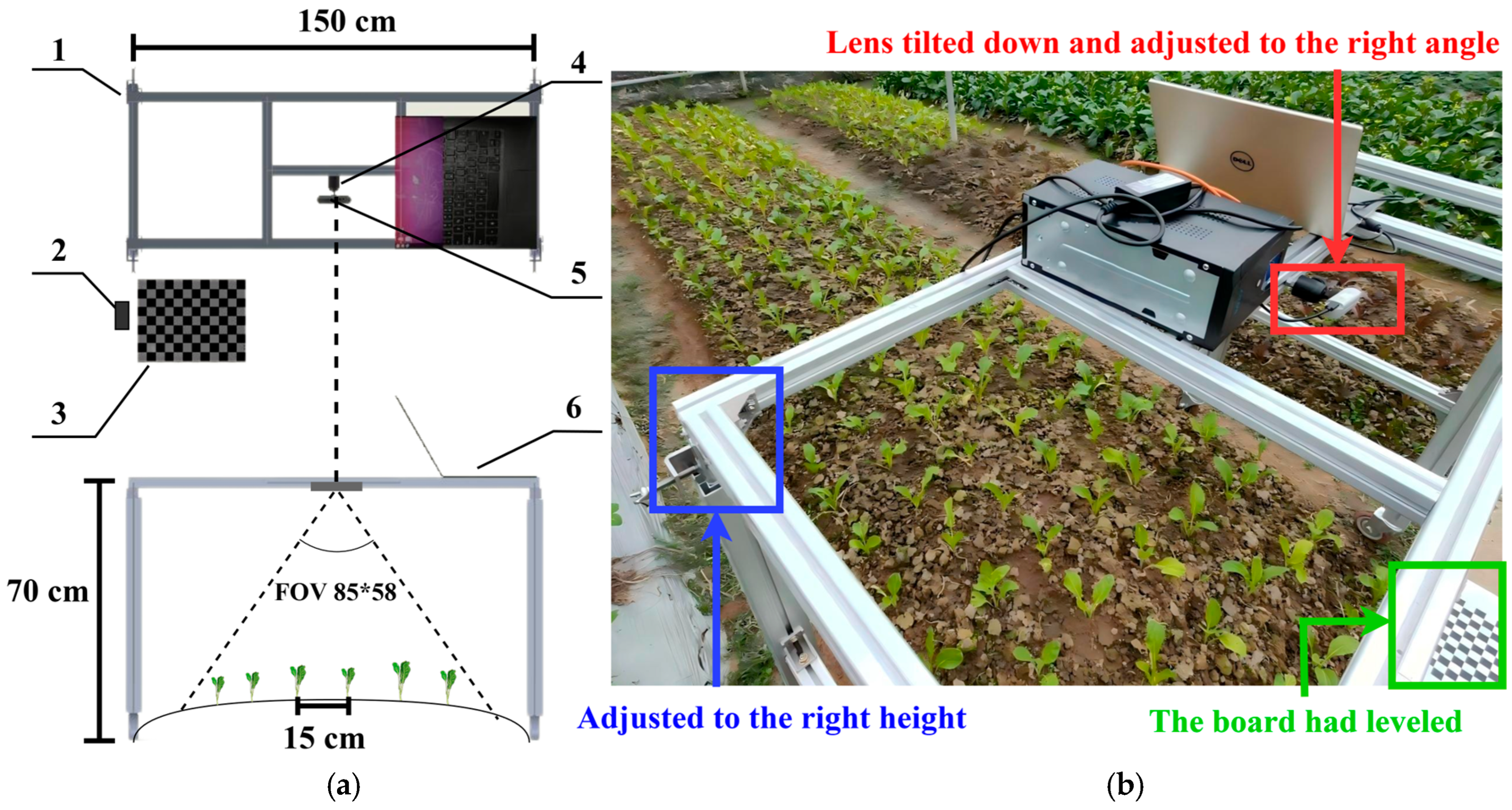
To ensure data consistency and minimize the influence of ambient light variations, all data were collected between 17:00 and 18:00, a time period with relatively low and stable light intensity, optimizing the quality of depth data. The data acquisition was performed using a custom-built mobile platform (Figure 1a,b), which was equipped with an Intel RealSense D435i depth camera (Intel Corporation, Santa Clara, CA, USA). Sensor control and data synchronization were managed within the Robot Operating System (ROS) framework on an Ubuntu 20.04 operating system.

Before data acquisition, the D435i camera underwent a detailed calibration process. The Kalibr toolkit was utilized for the intrinsic calibration of both the RGB camera and the infrared stereo module. Noise calibration of the built-in IMU was carried out using the imu_utils toolkit. A final joint calibration between the camera and IMU was conducted to align their coordinate systems. The accuracy of the depth data was verified using the official RealSense depth quality tool, which confirmed a Z-axis accuracy error of less than 0.6%. To enhance data quality, spatial filtering, temporal filtering, and hole-filling algorithms were employed to reduce noise and address missing data resulting from environmental conditions.

For establishing a consistent world coordinate system, a high-precision checkerboard calibration board was permanently fixed in the data collection area. The board was leveled with a spirit level to ensure vertical alignment with an error not exceeding 0.05°, serving as the spatial reference. The camera was mounted vertically downward on an adjustable stand, positioned 60–100 cm above the ground, and integrated with a mini pan-tilt unit to optimize its viewing angle. The platform traversed the target area at a constant speed of 10 cm/s, performing back-and-forth scans to generate comprehensive point clouds covering the entire ridge.

To validate the proposed method, the true height of each Choy Sum plant was manually measured using a digital caliper (accuracy: 0.02 mm), defined as the vertical distance from the root–stem junction (root collar) to the highest point of the canopy. Each measurement was repeated three times per plant, and the average value was taken as the reference height. Manual measurements were synchronized with point cloud acquisition to minimize errors caused by plant growth between sampling times. A total of 202 plants were monitored throughout the entire experimental period.

2.2. Overview of the Proposed Framework

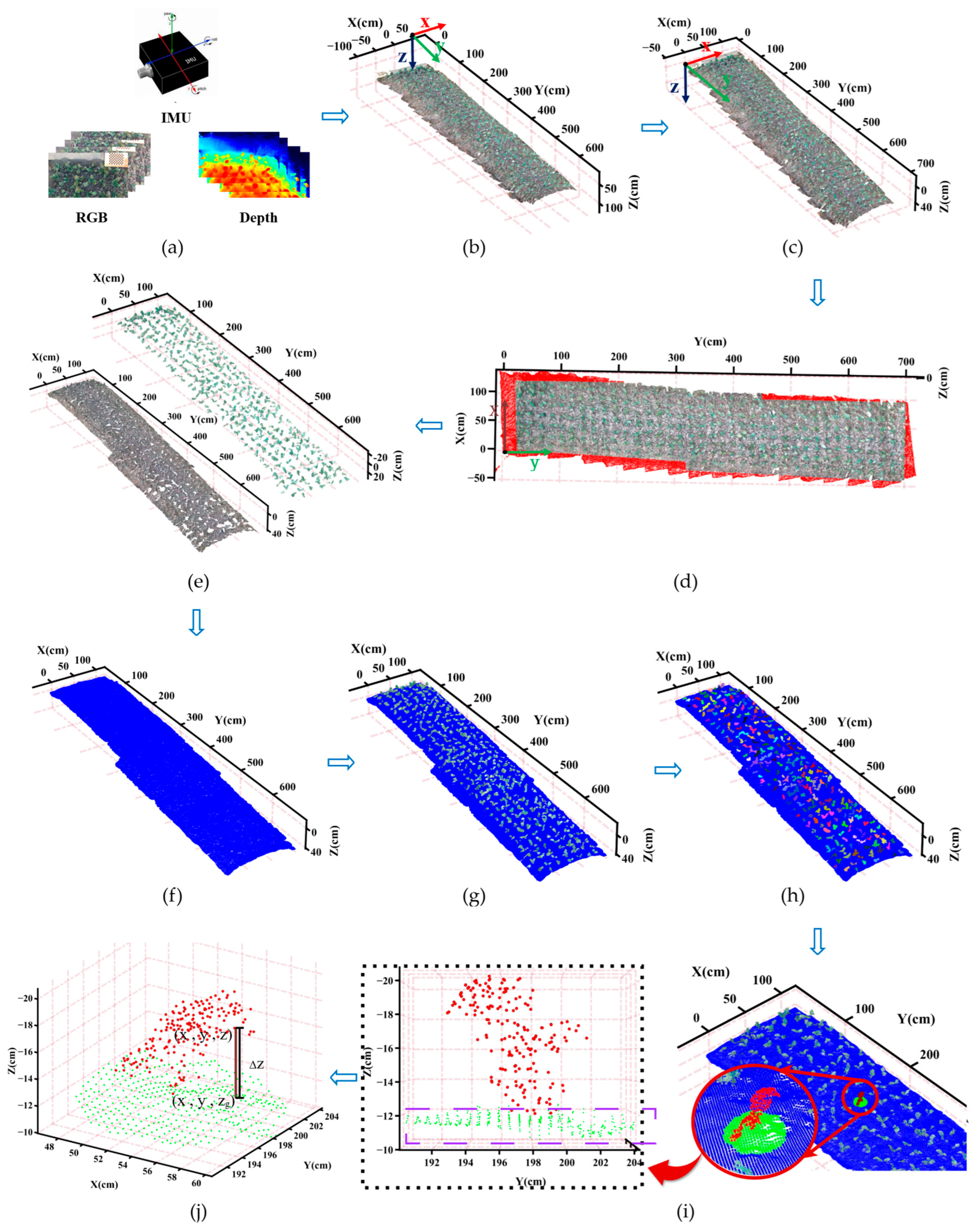
The proposed framework processes color images, depth images, and IMU data streams from an RGB-D camera to continuously monitor the plant height of Choy Sum (Brassica rapa var. parachinensis) throughout its entire growth cycle. The workflow is illustrated in Figure 2 and consists of three primary stages:

• Three-dimensional Point Cloud Reconstruction and Coordinate System Alignment
  Initially, a 3D point cloud map is reconstructed from the RGB-D data using an improved Oriented FAST and Rotated BRIEF–Simultaneous Localization and Mapping (ORB-SLAM3) algorithm (Figure 2b). A stable world coordinate system is then established based on a fixed checkerboard calibration board placed within the scene. The point cloud map is transformed into this unified coordinate system (Figure 2c). Subsequently, background points, including non-target point clouds, are filtered out (Figure 2d). This step ensures precise spatial alignment of multi-temporal point cloud datasets into a single, absolute reference frame through feature matching and coordinate transformation. Additionally, non-field objects, such as ridges and paths, are identified and removed based on their spatial relationship to the coordinate system and plot boundaries. Importantly, the Z-axis of the world coordinate system is orthogonal to the ground plane, providing a geometrically consistent foundation for subsequent Kriging interpolation and ground model reconstruction.
• Reference Ground Model Reconstruction and Multi-Temporal Point Cloud Alignment
  Given the short growth cycle of leafy vegetables, minimal ground deformation after transplantation, and the completeness of early-stage point clouds, ground points are initially extracted using color-based segmentation (Figure 2e). The ground point cloud from the early growth stage is selected as the reference. However, due to seedling occlusion and denoising processes, some ground points are missing. To address this, a continuous surface is reconstructed using Kriging interpolation (Figure 2f). The vegetable point clouds from each subsequent growth stage are then fused with this reference ground model (Figure 2g), providing the data needed for calculating plant height by determining the canopy-to-ground elevation difference.
• Plant Height Calculation Across the Growth Cycle
  Early Stage Measurement Area Delineation: For the early-growth stage, individual plants are segmented using a fast Euclidean clustering algorithm (Figure 2h). The measurement area for each plant is defined based on the extent of its canopy (Figure 2i).
  Late-Stage Measurement Area Delineation: During the late growth stage, when the leaves expand radially from the center, measurement areas are defined using the known planting spacing and the pre-determined center points from the early-stage areas.
  Coordinate Correction: The Random Sample Consensus (RANSAC) algorithm is applied to estimate the normal vector of the local ground plane within each measurement area. A rotational transformation is then applied to align this normal vector with the Z-axis of the world coordinate system, eliminating any systematic errors caused by pose misalignment (Figure 2i).

Height Computation: Finally, the plant height is calculated as the elevation difference between the highest canopy point and the reference ground model within the defined measurement area (Figure 2j).

2.3. Three-Dimensional Reconstruction and Point Cloud Preprocessing

2.3.1. Reconstruction of Open-Field Choy Sum Point Clouds Based on an Improved ORB-SLAM3 Algorithm

Previous studies have demonstrated the feasibility of using ORB-SLAM-based frameworks to measure crop height in open-field environments [14,25,26,27]. In this study, we employ the enhanced ORB-SLAM3 algorithm proposed by Li et al. [25] for 3D reconstruction of the agricultural field scene. This improved version incorporates a dense mapping module and a YOLOv8-based object detection module for dynamic object removal, effectively addressing the original framework’s limitations of generating only sparse maps and mitigating tracking errors caused by wind-induced plant movement. The specific workflow is as follows.

Prior to feeding images into the SLAM tracking thread, dynamic vegetable regions are detected and masked out via object detection, retaining only static background feature points for camera pose estimation. Subsequently, RGB images and depth maps are fused to generate colored 3D point clouds (containing X, Y, Z coordinates and RGB color information). IMU data is tightly coupled to refine the inter-frame transformation matrices during point cloud registration, enabling precise stitching of point clouds from multiple keyframes and reduction in redundant points in overlapping regions. Finally, loop closure detection and global bundle adjustment are applied to construct a large-scale, metrically consistent, dense point cloud map (Figure 2b). This approach maintains the high real-time performance of ORB-SLAM3 while significantly enhancing the geometric completeness, density, and robustness of the reconstructed scenes, providing a reliable data foundation for subsequent plant height measurement.

2.3.2. World Coordinate System Unification and Background Removal

In outdoor agricultural 3D modeling, coordinate registration methods based on ground control points (GCPs) are well-established [11,17,28]. For instance, Jamil et al. [11] utilized 10 GCPs placed 53 m apart to achieve centimeter-level Digital Terrain Model (DTM) modeling, a technique suited for large-scale scenarios (>50 m). In contrast, for the small-scale experimental field in this study (with both length and width < 7 m), we propose an alternative method for constructing a coordinate system based on a visual calibration target.

An 8 × 11 checkerboard calibration board was employed as the reference for the world coordinate system. The board was carefully leveled using a spirit level, ensuring a verticality error of less than 0.05°. Feature points were then detected with high precision using the Harris corner detection algorithm, resulting in a single-point pixel error of less than 1.2 px. Leveraging the camera calibration results from Section 2.1, we applied the EPnP algorithm [29] to solve the rigid transformation parameters from the world coordinate system to the camera coordinate system. This included the rotation matrix R ∈ SO(3) and translation vector T ∈ R³, which together define the transformation that maps any world coordinate point P $=$ [X_W, Y_W, Z_W] ^T to its corresponding camera coordinate p $=$ [X_C, Y_C, Z_C] ^T, as described by Equation (1).

In small-scale scenarios, this method can effectively satisfy the requirements for coordinate transformation. However, as the spatial scale increases, it becomes necessary to employ multiple calibration boards or GCPs to achieve large-area map calibration (Section 3.1 for the relevant error analysis).

$$\mathit{p} =\mathit{R} · \mathit{P} +\mathit{T}$$

(1)

A point p in the camera coordinate system is transformed back to the world coordinate system as Q = [X, Y, Z] ^T, which corresponds to the actual 3D location of the physical calibration corner. The effect of this coordinate transformation is illustrated in Figure 2c, and the transformation formula is provided in Equation (2).

$$\mathit{Q} ={\mathit{R}}^{ -1} · \left(\mathit{P} - \mathit{T} \right)$$

(2)

The initial point cloud contained non-field objects (e.g., ridges, pathways, and the calibration board) and exhibited boundary artifacts from multi-frame stitching (indicated by the red areas in Figure 2d). To remove these artifacts and background elements, a two-step filtering pipeline was implemented. First, spatial threshold filtering, based on the known physical dimensions of the experimental plot, was applied to remove the majority of non-target points. Second, anisotropic Gaussian filtering was used to smooth jagged edges, followed by connected component analysis to isolate and retain only the point cloud corresponding to the planting area. This workflow effectively achieves both coordinate system unification and background removal, providing a clean and consistent spatial reference for subsequent analysis.

2.4. Plant and Ground Segmentation with Reference Surface Reconstruction

The acquired 3D point cloud contained mixed data of plants and the ground, requiring effective segmentation to extract distinct plant and ground information. The short growth cycle of leafy vegetables, minimal ground deformation after transplantation, and the high completeness of the early-stage ground point cloud made this period ideal for establishing a persistent reference surface, providing reliable ground elevation data for subsequent continuous plant height measurement.

2.4.1. Plant-Ground Segmentation

The raw point cloud was initially denoised. Discrete noise was addressed using the Statistical Outlier Removal (SOR) algorithm [30], which analyzes the local point density around each point to identify and remove statistical outliers, resulting in a smoother point cloud. Given the standardized field management (weed-free) and the optimal data acquisition period (low ambient light interference), the pre-processed point cloud predominantly consisted of the ground surface and Choy Sum plants.

Plant-ground segmentation was performed using color-depth fusion data from the RGB-D camera, based on chromaticity analysis. After evaluating performance across multiple color spaces (RGB, HSV, and YCrCb), the Excess Green (ExG) index in the RGB space (Figure 2e) proved most effective for this application. The ExG index leverages the chlorophyll reflection properties, which cause plant points to exhibit a stronger green (G) channel response, while the soil surface typically shows a dominant red (R) channel response, allowing for reliable separation between plants and ground.

The segmentation result contained two primary types of noise:

• High-frequency jagged noise at the leaf-ground boundary, caused by perspective projection and spectral aliasing, which risked misclassification as ground points.
• Discrete outliers from green pixels projected onto the ground, which could be misidentified as plant points.

To address these, anisotropic filtering [31] was applied to smooth the edge artifacts, while radius filtering (search radius: 5 cm; minimum neighbors: 20; these parameters were finalized through iterative testing and visual evaluation; specific values should be adjusted according to individual application requirements) [32] was used to remove the discrete outliers. This resulted in high-fidelity plant and ground segmentation, ready for further analysis.

2.4.2. Surface Reconstruction

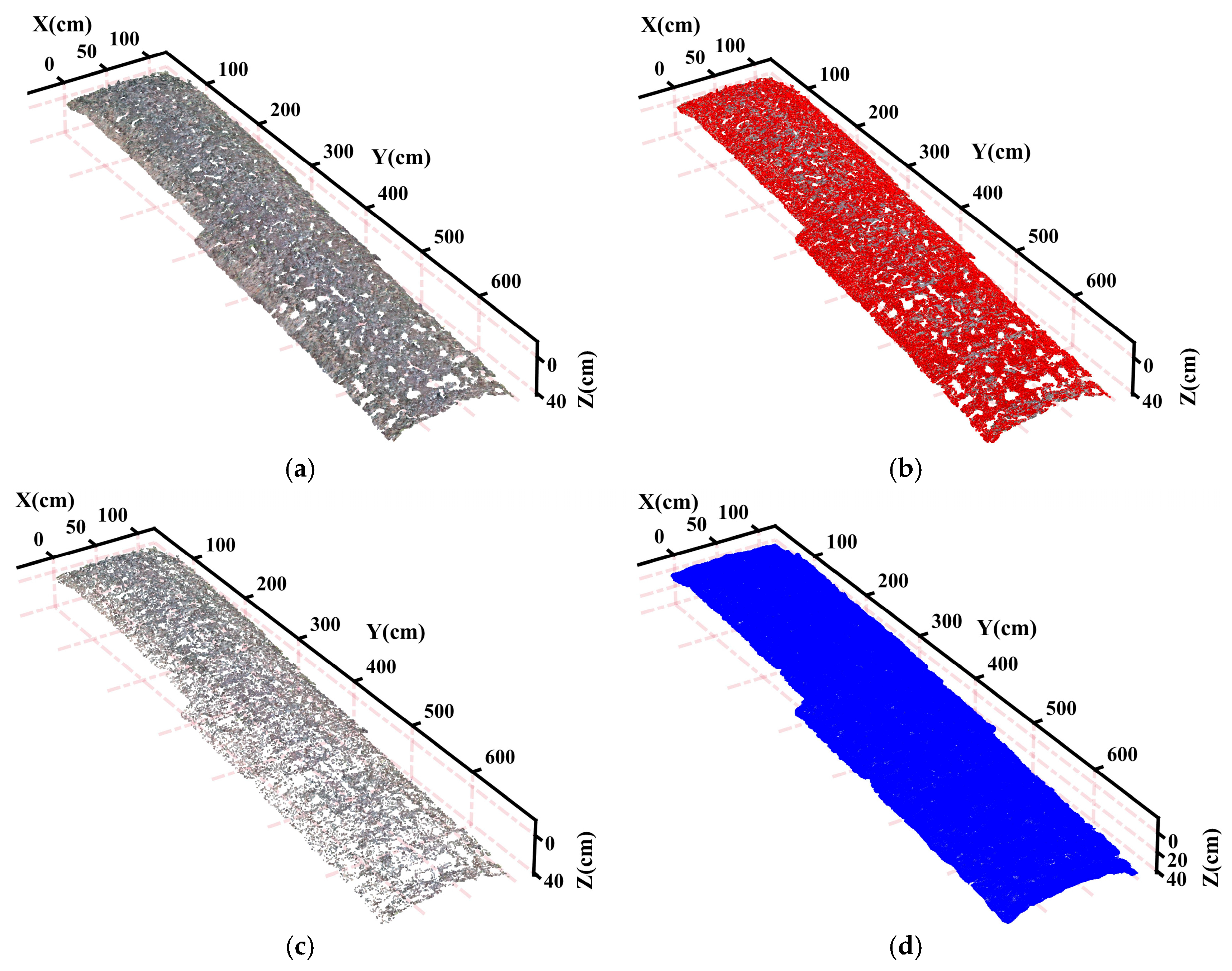
The reference ground surface was reconstructed in two stages: ground point cloud filtering and surface interpolation (Figure 3).

First, the Cloth Simulation Filter (CSF) algorithm [33] was applied. This algorithm simulates a virtual cloth settling under gravity onto the inverted point cloud, utilizing the geometric continuity of the ground to adaptively separate and remove residual vegetation and debris (Figure 3c).

Next, to address localized gaps in the filtered ground point cloud, Kriging interpolation [34] was employed to reconstruct a continuous terrain surface. This geostatistical method models the spatial autocorrelation of elevation data via a semivariogram. A Gaussian covariance function and least-squares criteria were used to optimize the spatial weighting for interpolation. Simultaneously, a standard deviation field was generated to quantify spatial uncertainty (Figure 3d). Compared to deterministic interpolation methods, Kriging interpolation not only effectively fills data gaps but also provides an error estimate for subsequent plant height measurements. The result is a high-precision, continuous DTM that serves as the ground reference.

2.5. Multi-Temporal Point Cloud Fusion

This stage focuses on fusing the reconstructed reference ground model (described in Section 2.4.2) with the plant point clouds collected across different time periods. The fusion process varies significantly between the early and late growth stages.

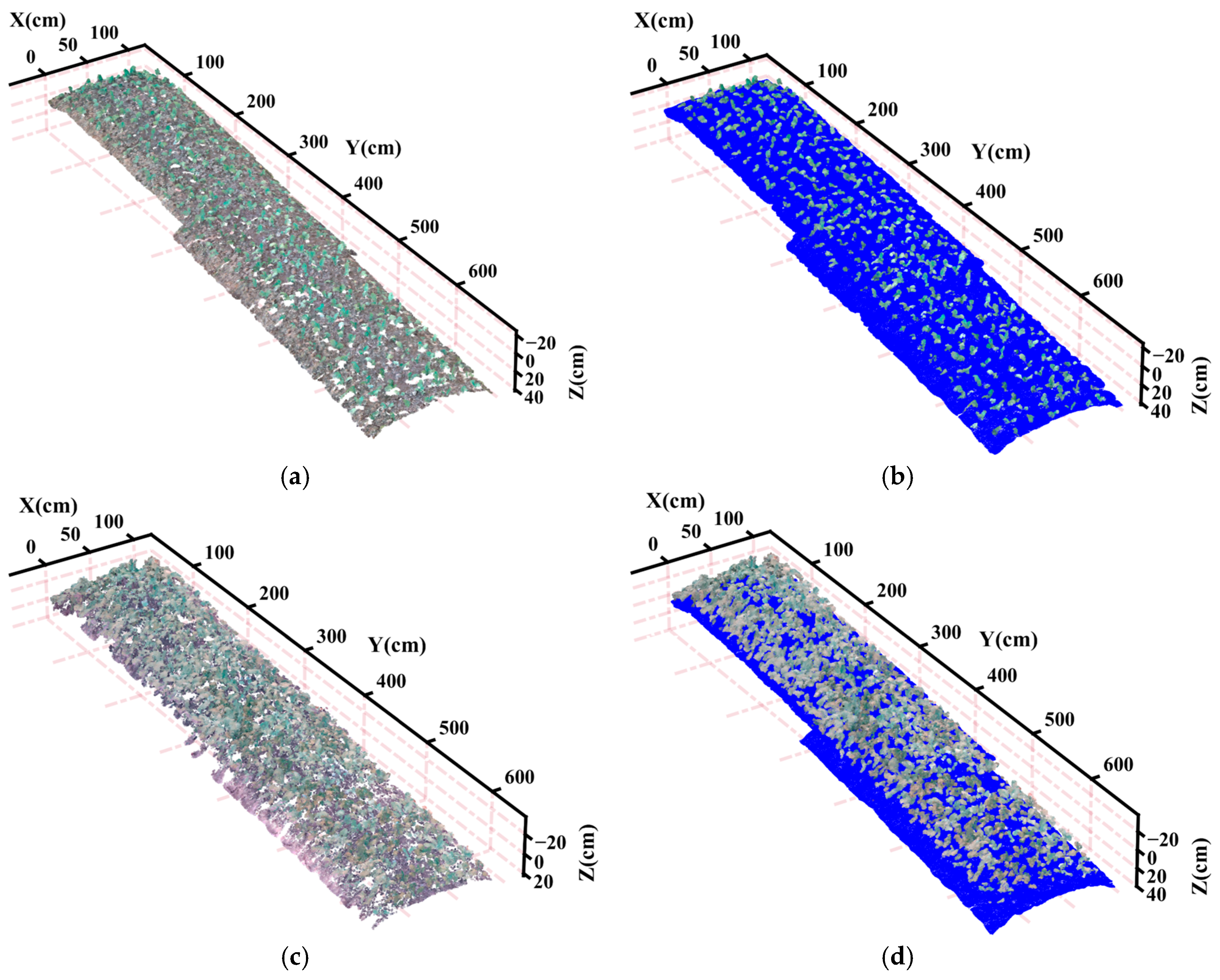
In the early growth stage, both the reference ground model and the plant point clouds come from data captured in the same acquisition sequence (Figure 4a). As a result, they are inherently aligned in the same coordinate system, introducing no additional spatial registration errors (Figure 4b). The fusion of these datasets enhances the integrity of the ground surface, ensuring high accuracy for plant height measurements.

In the late growth stage, the reference ground model, derived from early-stage data, is fused with plant point clouds from a later period. This requires cross-temporal registration, using the Harris corner detection and EPnP algorithms outlined in Section 2.3.2. This process introduces some spatial alignment error (see Section 4.1 for quantitative error analysis). As shown in Figure 4c, the ground in the original point cloud is heavily occluded by the dense canopy and contains substantial noise, making it unsuitable for direct measurement. In contrast, after multi-temporal fusion (Figure 4d), the ground reference is effectively recovered, providing a reliable and accurate reference surface for plant height calculation.

2.6. Plant Height Extraction

2.6.1. Measurement Region Delineation and Coordinate Correction

Accurate measurement of individual plant height requires the delineation of a measurement region for each plant and applying a coordinate correction to eliminate systematic errors induced by local ground slope. As outlined in Section 2.2, the strategy for defining this region differs between the early and late growth stages.

Necessity of geometric formulations. The introduction of Equations (1)–(7) is essential to ensure consistent and accurate plant height estimation across multiple growth stages. Specifically, Equations (1) and (2) transform all reconstructed point clouds into a unified world coordinate system defined by the fixed checkerboard, which is a prerequisite for multi-temporal alignment. Equations (3)–(7) further address local ground inclination and pose-induced bias by aligning the fitted local ground plane with the global vertical (Z-axis). Without these geometric transformations and corrections, canopy-to-ground height differences would be affected by coordinate drift and local terrain slope, leading to systematic errors, particularly during late growth stages when multi-temporal fusion is required.

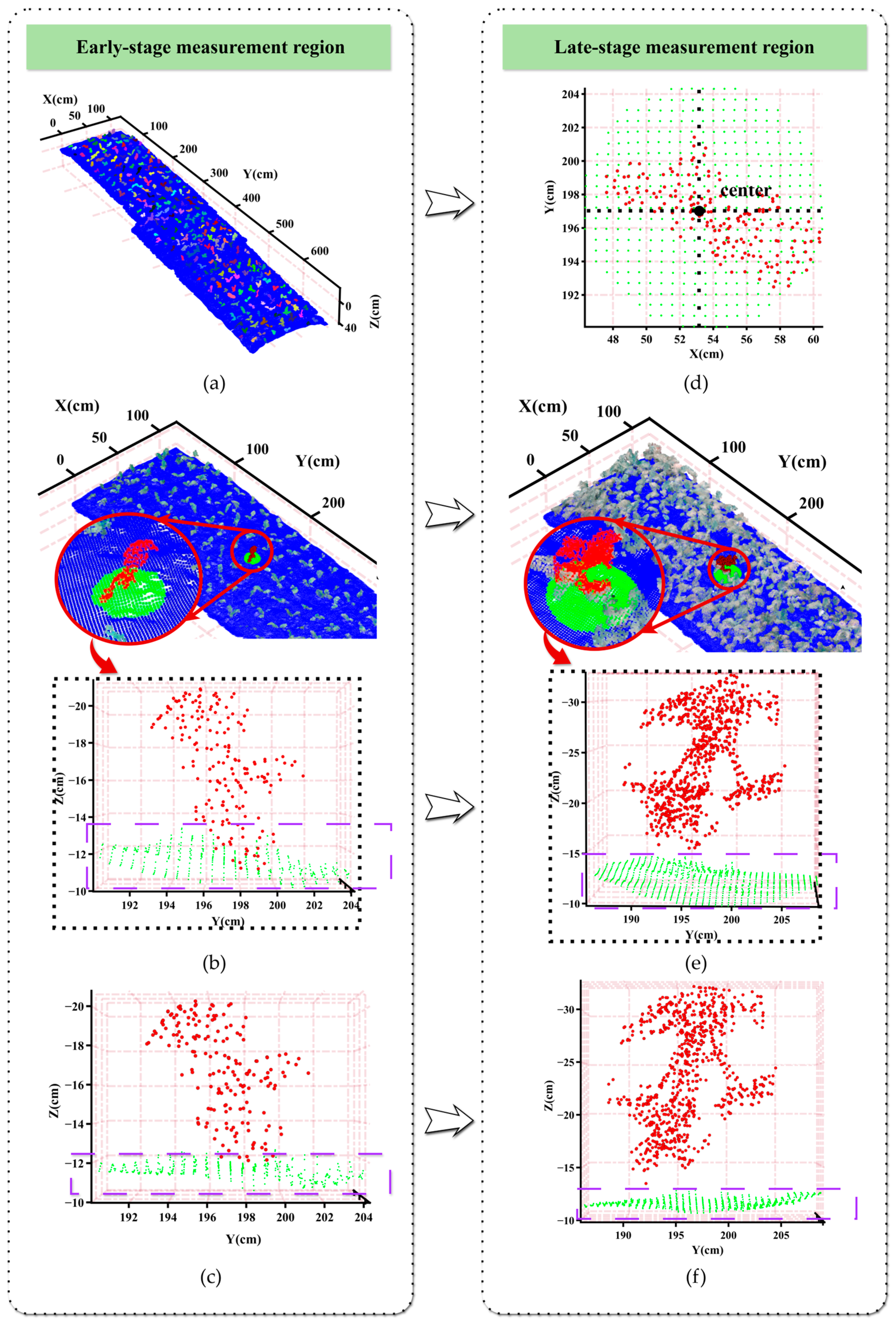
In the early stage of vegetable growth, the distance between plants is relatively large, making it easy to distinguish individual plants. A fast Euclidean clustering algorithm is first employed to segment the point cloud, effectively isolating individual plants (Figure 5a), with distinct colors representing each plant. Next, based on the projection of a plant’s canopy points onto the XY plane of the world coordinate system, a circular measurement region, slightly larger than the canopy extent, is automatically delineated. This region contains both the plant’s points and the corresponding portion of the reconstructed reference ground model (Figure 5b).

To mitigate measurement bias due to local ground slope, a coordinate correction is applied. The RANSAC algorithm is used to fit a plane to the local ground points within the delineated region, defined by the equation:

$$\mathrm{A}\mathbf{X} + \mathrm{B}\mathbf{Y} + \mathrm{C}\mathbf{Z} + \mathrm{D} = 0$$

(3)

where n $=$ (A, B, C) is the normal vector of the fitted plane and D is the distance from the origin to the plane. The angle θ between this normal vector and the world coordinate system’s Z-axis vector k $=$ (0, 0, 1) is computed using the dot product formula:

$$\mathit{\theta } = \arccos \left(\left(\mathit{n} · \mathit{k}\right)/\left(‖\mathit{n} ‖ \times ‖\mathit{k} ‖\right)\right)$$

(4)

The axis of rotation $\mathit{c}$ is determined by the cross product of vectors n and k:

$$\mathit{c} = \mathit{n}\times \mathit{k}$$

(5)

Let u be the unit vector in the direction of c (i.e., $\mathit{u} = \mathit{c} /‖\mathit{c} ‖$). Using the angle θ obtained above, the rotation matrix R_rot that aligns the RANSAC-fitted plane with the world coordinate XY plane is computed using the Rodrigues’ rotation formula:

$${\mathit{R}}_{\mathit{rot}} = \mathrm{I} + \mathbf{sin}\mathit{\theta } ·{\left[\mathit{u}\right]}_{\times } + \left(1 - \mathbf{cos}\mathit{\theta }\right)·{{\left[\mathit{u}\right]}_{\times }}^2$$

(6)

where I is the 3 × 3 identity matrix and ${\left[\mathit{u}\right]}_{\times }$ is the skew-symmetric matrix form of vector u. Let P_o ∈ R^{3 × N} denote the original point cloud, where each column corresponds to a 3D point in homogeneous coordinates. The corrected point cloud P_c is then obtained by applying this rotation matrix:

$${\mathit{P}}_{\mathit{c}} = {\mathit{R}}_{\mathit{rot}} · { \mathit{P}}_{\mathit{o}}$$

(7)

where t P_c ∈ R^{3 × N} represents the rotated point cloud aligned with the XY plane. The coplanarity between the local ground surface and the world coordinate system’s XY-plane is significantly enhanced in the corrected point cloud (as shown by comparing Figure 5b,c,e,f), thereby providing a more reliable reference benchmark for subsequent plant height measurement.

During the late growth stage, severe canopy closure and mutual leaf occlusion make it impossible to automatically delineate measurement regions through projection. To overcome these challenges, our approach leverages two key characteristics: the fixed planting spacing of Choy Sum (15 cm) and its radial leaf expansion pattern from the center.

The previously acquired center coordinates of individual plants from the early growth stage (Figure 5d) served as anchor points for the late-stage measurements. We manually delineated circular measurement regions centered on these coordinates (Figure 5e) and applied the identical coordinate correction methodology described previously (Figure 5f). This strategy ensures measurement consistency across growth stages and significantly improves the reliability of plant height extraction during the critical late growth phase.

Although Equations (1)–(7) are based on standard geometric formulations widely used in computer vision and point cloud processing, they are indispensable in the proposed framework. Their systematic integration explicitly enforces multi-temporal coordinate consistency, vertical height normalization, and local ground inclination correction. This ensures that plant height is always measured along a unified and physically meaningful vertical direction, even under uneven terrain and severe canopy occlusion in later growth stages.

2.6.2. Plant Height Calculation

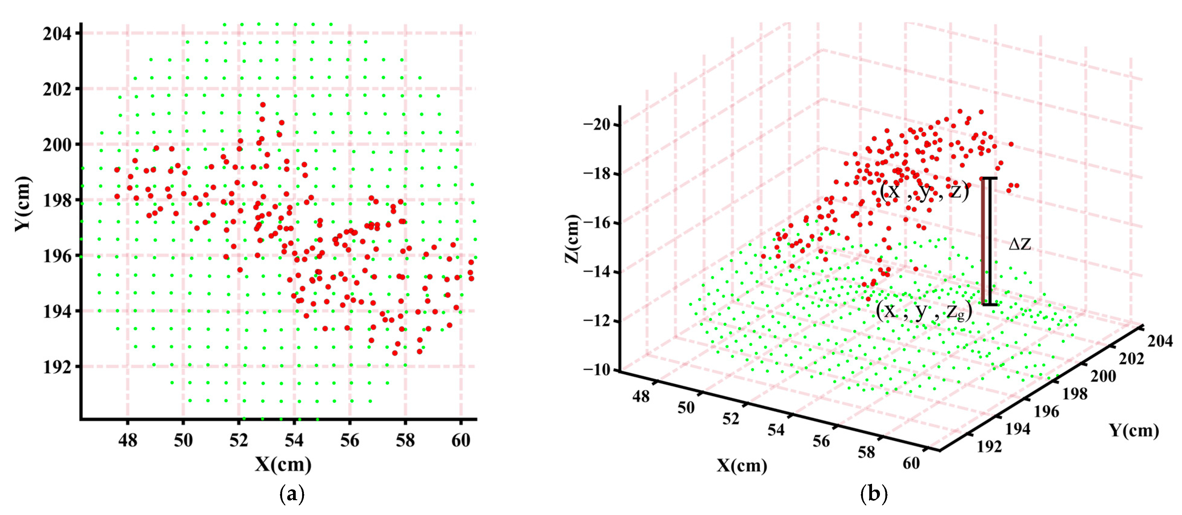
Plant height is determined by calculating the maximum vertical distance between the canopy points and the reference ground surface within the coordinate-corrected measurement region for each plant. The calculation process begins by considering an individual canopy point with coordinates (x, y, z). To estimate the ground elevation directly beneath this point, the method first projects the point onto the XY-plane at coordinate (x, y). Since no ground point exists exactly at this projected location due to non-overlapping distributions of canopy and ground points after correction (Figure 6a), the algorithm identifies the four nearest neighboring ground points to (x, y) in the XY-plane. The average z-coordinate of these four points, denoted as z_g, is computed to generate an interpolated ground point at (x, y, z_g).

The vertical distance from the canopy point to the ground is then calculated as Δz (Figure 6b):

$$\Delta \mathrm{z} = \left|\mathrm{z} - {\mathrm{z}}_{\mathrm{g}}\right|$$

(8)

This process is repeated for all canopy points within the measurement region, generating a set of vertical distance values. The final plant height H is determined as the maximum value from this set of calculated Δz values, representing the highest point of the plant relative to the reconstructed ground surface beneath it.

Plant height measurement methods are typically validated by comparing automated results with manual ground-truth values using MAE and R². This study adopts the same evaluation metrics to assess method accuracy.

3. Results

3.1. Terrain Error Analysis

To address missing data in the original ground point cloud and to select an appropriate interpolation method, terrain reconstruction accuracy was compared between the Inverse Distance Weighting (IDW) method and Kriging, using the ground data described in Section 2.4.2. Due to gaps in the sampled ground points, interpolation was required to generate a continuous reference surface.

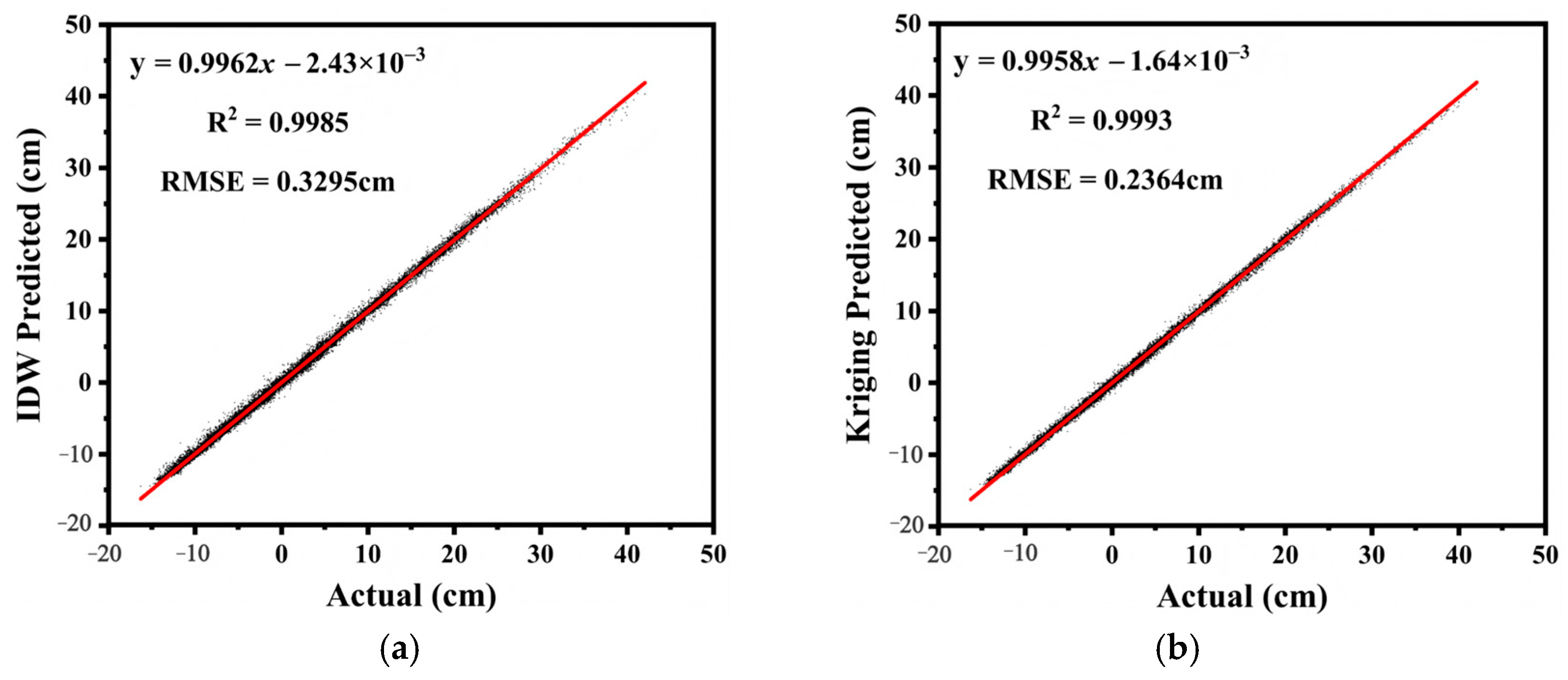
For a fair comparison, 45,086 points were uniformly sampled from the interpolated surfaces of both methods using nearest-neighbor search, and their elevation errors were computed against the corresponding original ground points. The error distributions are shown in Figure 7. Kriging produced scatter points that were more concentrated around the regression line (Figure 7b), with an RMSE of 2.364 mm, which was lower than that of IDW (3.295 mm). Therefore, Kriging was used for terrain reconstruction in subsequent analyses.

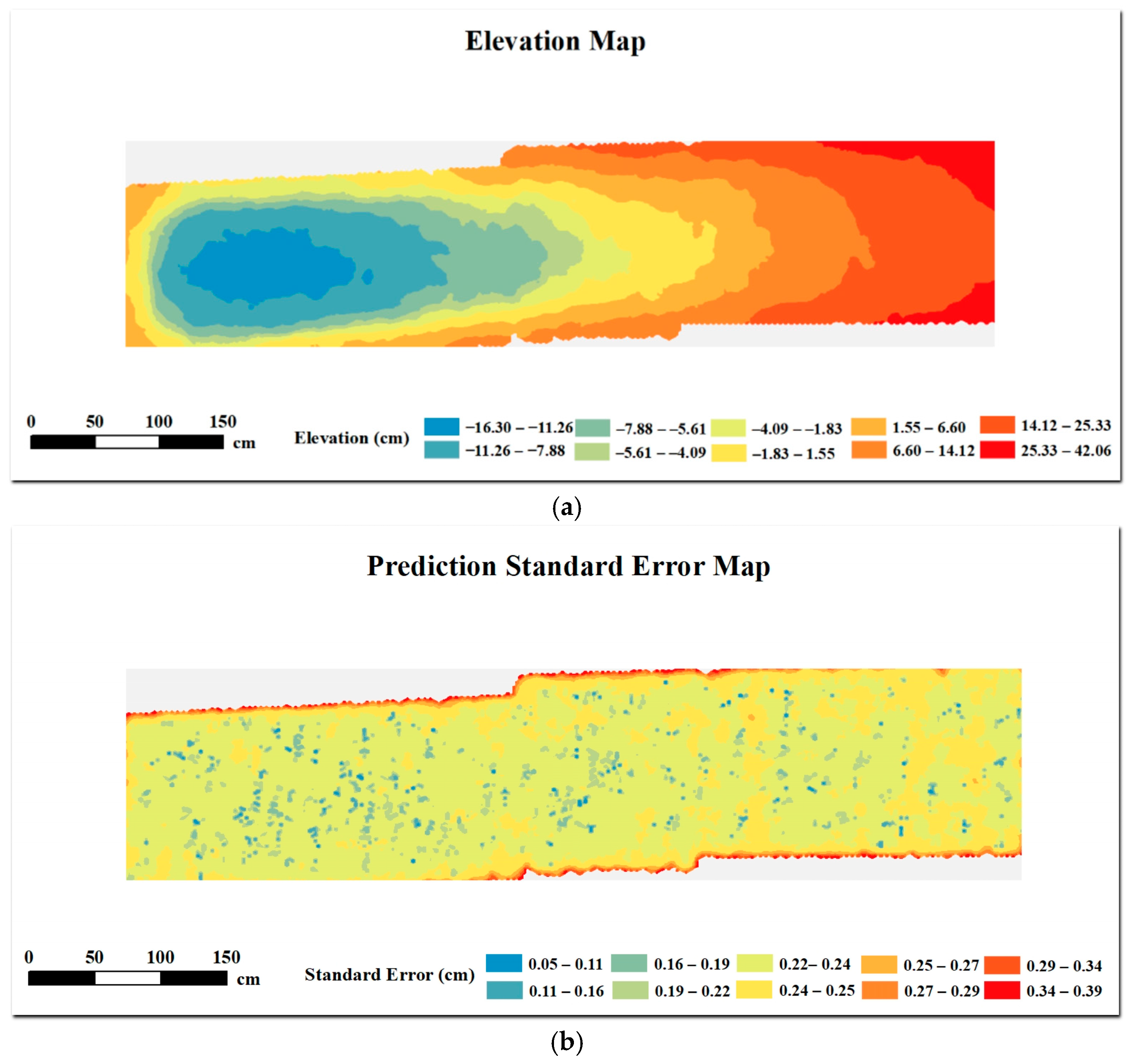
To further characterize the Kriging-based terrain reconstruction, an elevation distribution map and a prediction standard error map were generated (Figure 8a,b). The elevation map indicates that terrain height ranges from −16.30 cm to 42.06 cm, with a total relief of 58.36 cm across the experimental plot (Figure 8a). The prediction standard error map shows lower uncertainty in the interior regions (2.2–2.5 mm) and higher uncertainty near plot boundaries (2.5–3.9 mm), consistent with the spatial distribution of available ground points (Figure 8b).

Overall, Kriging interpolation achieved an R² of 0.9993 with an RMSE of 2.364 mm. Most interior areas exhibited prediction standard errors between 2.2 mm and 2.5 mm, while higher uncertainty was observed near the plot edges.

3.2. Plant Height Measurement Analysis

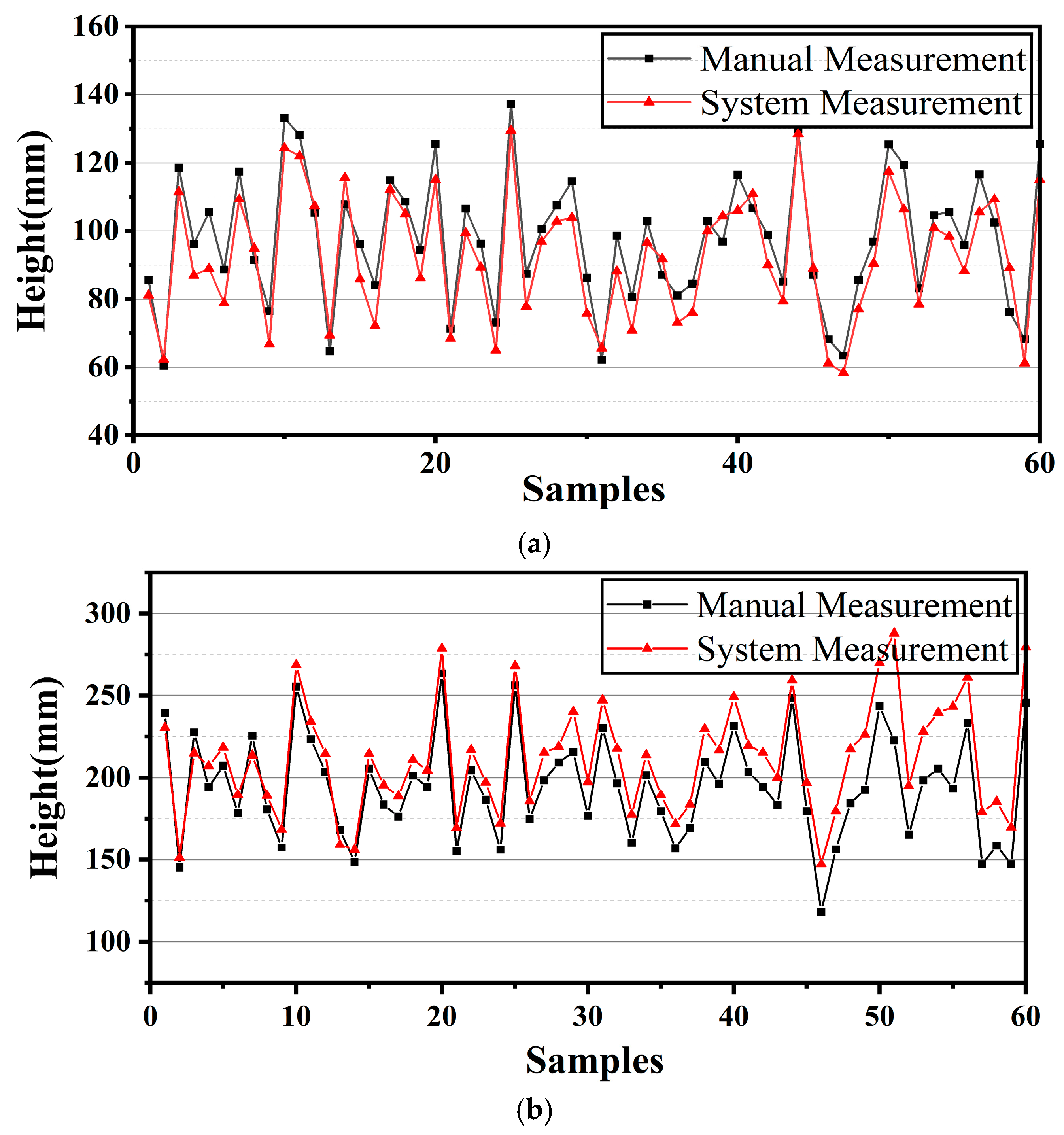
Continuous data collection was conducted over a 25-day period following the transplantation of Choy Sum, covering key growth stages from day 5 to maturity. To represent early and late growth conditions, point cloud data acquired on day 9 and day 21 after transplantation were selected for plant height evaluation.

The experimental field contained 202 plants with complete data at both time points. Due to the requirement of manual delineation of measurement regions during the late growth stage, 60 plants were selected for quantitative evaluation using a sampling strategy. Specifically, 10 plants were selected at 1 m intervals from near to far relative to the checkerboard calibration target.

Plant height was estimated using a terrain-referenced point cloud–based algorithm, in which a Kriging-interpolated ground surface served as the reference terrain model. For each plant, height was calculated as the vertical difference between canopy points and the corresponding terrain elevation within the defined measurement region, as described in Section 2.6.

To further evaluate the contribution of key components in the proposed framework, a component analysis was conducted based on plant height estimation accuracy. A direct ablation that removes the reference ground model is not feasible for late growth stages because the ground surface is severely occluded in the raw RGB-D point clouds, making canopy-to-ground height computation ill-posed without a persistent ground reference.

Therefore, the analysis focuses on components that can be evaluated under the same experimental setting. Specifically, we compared the full proposed method with a variant in which the local ground plane correction was disabled. In the ablated variant, plant height was computed directly using the original world coordinate system without applying the RANSAC-based plane fitting and rotation alignment.

The comparison results are summarized in

Table 1. Component analysis of plant height estimation accuracy.

Method	Early-Stage MAE (mm)	Late-Stage MAE (mm)	R2 (Late Stage)
Full proposed method	7.19	18.45	0.855
Without local plane correction	8.13	24.63	0.692

. Removing the local plane correction leads to increased estimation error, particularly under uneven terrain conditions, demonstrating that local plane normalization plays an important role in ensuring accurate and robust plant height estimation.

The comparison between estimated plant height and manual measurements is shown in Figure 9. Strong correlations were observed at both growth stages, with coefficients of determination (R²) of 0.902 for the early stage and 0.855 for the late stage. The mean absolute error (MAE) was 7.19 mm in the early growth stage and 18.45 mm in the late growth stage.

4. Discussion

4.1. Impact of Coordinate Transformation Errors on Plant Height Estimation

The accuracy of plant height estimation in the proposed framework is closely related to the quality of coordinate transformation during multi-temporal point cloud alignment. Although all point clouds are transformed into a unified world coordinate system (WCS) defined by a fixed checkerboard calibration board, residual transformation errors can still propagate into height measurements under specific conditions.

In the early stage of growth, both the reference ground surface and plant point clouds are acquired within the same data collection sequence and transformed into the WCS using identical transformation parameters. As a result, relative height measurements between the canopy and ground are preserved, and coordinate transformation errors do not significantly affect plant height estimation at this stage.

In contrast, during the later growth stages, the reference ground model reconstructed from early-stage data must be fused with plant point clouds acquired at later time points. Because these datasets undergo independent coordinate transformations, residual errors in camera pose estimation and transformation parameters directly influence the accuracy of canopy-to-ground height differences. This effect becomes more pronounced as the distance between the target plant and the calibration board increases, consistent with the error propagation characteristics of the pinhole camera model [29].

This distance-dependent error behavior explains the increasing residual magnitude and variability observed for plants located farther from the checkerboard in Figure 9b. Although the adopted coordinate transformation strategy provides sufficient precision for small-scale field plots, the accumulation of residual transformation errors represents a dominant source of uncertainty in late-stage plant height estimation when multi-temporal fusion is required.

Overall, the experimental results indicate that coordinate transformation errors have a negligible impact on early-stage measurements but become an important limiting factor for late-stage plant height estimation. By constraining the measurement area and using a fixed calibration reference, the proposed framework maintains measurement accuracy within acceptable limits for field-grown leafy vegetables. For larger measurement areas, additional spatial reference constraints would be required to suppress error accumulation.

4.2. Influence of Terrain Reconstruction Accuracy on Plant Height Estimation

Accurate terrain reconstruction is a prerequisite for reliable plant height estimation in open-field environments with uneven ground surfaces. In the proposed framework, plant height is defined as the vertical difference between canopy points and a reconstructed reference terrain surface. Consequently, any error in terrain elevation directly propagates into the estimated plant height.

As shown in Figure 8a, the experimental plot exhibits a vertical terrain relief of 58.36 cm, which is comparable to or exceeds the height of mature leafy vegetables. Under such conditions, assuming a flat or locally uniform ground surface would lead to systematic bias in canopy-to-ground height estimation. The Kriging-based terrain reconstruction provides a continuous reference surface that preserves local elevation variations and reduces this source of error.

The prediction standard error map in Figure 8b further indicates that terrain reconstruction uncertainty is spatially heterogeneous. Lower standard errors are observed in interior regions with dense ground point coverage, while higher uncertainty occurs near plot boundaries where ground data are sparse. This spatial pattern implies that plant height estimation is more sensitive to terrain reconstruction accuracy in edge regions, which should be considered when interpreting measurement results.

Overall, the terrain reconstruction accuracy achieved in this study (RMSE = 2.364 mm) provides a stable and sufficiently precise ground reference for plant height estimation at the centimeter scale. When combined with multi-temporal point cloud alignment, this approach enables reliable canopy-to-ground height measurement even under conditions of severe canopy occlusion during later growth stages.

4.3. Overall Performance and Comparison with Existing Methods

The results presented in this study demonstrate that reliable plant height estimation for field-grown leafy vegetables can be achieved across the full growth cycle, despite the challenges posed by dense canopy occlusion and uneven terrain. This capability is particularly important for short-stature crops with high planting density, where ground visibility rapidly decreases during later growth stages and conventional ground-referenced methods become unreliable.

Building upon previous studies by Obanawa, Dong, Zhang, and colleagues [12,13,22], this study adopts the canopy-to-ground height difference as the basis for plant height estimation, thereby avoiding the need for full-plant reconstruction. Compared with LiDAR-based or multi-view stereo approaches, which often require expensive hardware or are sensitive to canopy occlusion, the proposed framework leverages RGB-D sensing and multi-temporal point cloud alignment to balance measurement accuracy and system practicality under open-field conditions.

Several design choices contribute to the observed performance. The use of a fixed checkerboard calibration target provides a stable local spatial reference, enabling accurate coordinate unification in small field plots without relying on GPS. In addition, the reconstruction of a persistent reference ground surface from early-stage data allows plant height estimation to remain feasible even when the ground is fully occluded during later growth stages. This temporal decoupling of ground modeling and canopy measurement distinguishes the proposed method from frame-level RGB-D approaches that are typically limited to early growth stages.

Under consistent growth conditions, the proposed method achieved a mean absolute error of 7.19 mm in the early growth stage, which is lower than the 9.23 mm reported by Zhao et al. [22] for lettuce height measurement in a potted environment. Although direct numerical comparison across studies should be interpreted with caution due to differences in crop type and experimental setup, this result indicates that the proposed framework can achieve competitive accuracy in open-field environments characterized by uneven terrain and severe canopy occlusion. More importantly, the method uniquely supports continuous monitoring throughout the entire growth cycle, which remains a key limitation for many existing RGB-D–based plant height measurement approaches.

A quantitative comparison between the proposed method and representative state-of-the-art approaches is summarized in

Table 2. Performance comparison of plant height estimation methods using different sensing modalities and experimental setups.

Study	Sensor Type	Experimental Environment	Crop Type	Growth Stage	MAE (mm)	R2
Obanawa et al. [13]	LiDAR	Grassland	Italian ryegrass	Single	–	–
Dong et al. [12]	RGB-D	Field	Row crops	Multi-temporal	–	–
Qiu et al. [18]	RGB-D	Field	Maize	Jointing	–	>0.95
Zhao et al. [20]	RGB-D	Potted (Indoor)	Lettuce	Early	9.23	0.89
Zhang et al. [22]	Multi-view RGB	Open Field	Oat	Single	23.0 avg/22.4 max	–
Jiang et al. [23]	RGB-D	Field	Cotton	Canopy development	–	0.35–0.71
This study	RGB-D	Open Field	Choy Sum	Full Growth Cycle	7.19/18.45	0.902/0.855

. Although direct numerical comparison is constrained by differences in crop type, sensor configuration, and experimental conditions, the proposed framework achieves competitive accuracy while uniquely supporting continuous plant height monitoring throughout the entire growth cycle under open-field conditions with dense canopy occlusion.

To further differentiate the proposed approach from existing plant height estimation methods, qualitative aspects related to sensing modality, platform characteristics, reference and alignment strategies, as well as cost and computational considerations, are summarized in

Table 3. Comparison of representative plant height measurement methods in terms of methodology and applicability.

Study	Method	Platform	Reference and Alignment	Efficiency and Cost	Applicability
Obanawa et al. [13]	LiDAR/SfM geometry-based	UAV	Canopy surface differencing	High hardware cost	Grassland; not designed for dense leafy vegetables
Dong et al. [12]	Spatio-temporal SfM/MVS (4D reconstruction	UAV	Multi-temporal 3D model alignment	Low sensor cost, high computation	Row crops; sensitive to occlusion
Qiu et al. [18]	RGB-D frame-level height extraction	Ground	Visible ground reference per frame	Low cost, simple pipeline	Early growth stage only
Zhao et al. [20]	Depth vision + instance segmentation	Ground	Depth-based bottom plane reference	Low cost, moderate computation	Lettuce; dense leafy vegetables (single stage)
Zhang et al. [22]	CNN-based regression on depth images	Ground	Learned depth–height mapping	Low sensor cost, high computation	Cereal crops; limited for leafy vegetables
Jiang et al. [23]	RGB-D canopy profiling	Ground	Canopy surface relative to ground	Low cost, moderate computation	Field crops; not optimized for dense canopies
This study	Multi-temporal RGB-D point cloud alignment	Ground	Persistent reference ground + unified coordinate system	Low-cost sensor, moderate computation	Dense leafy vegetables; full growth cycle

.

4.4. Limitations and Future Research Directions

Despite the promising performance of the proposed framework, several limitations should be acknowledged. First, although the use of a persistent reference ground surface alleviates the impact of ground occlusion, extremely dense or overlapping canopies may still affect the accurate delineation of individual plant regions, particularly during late growth stages with severe inter-leaf occlusion. Second, the performance of RGB-D sensors is inherently sensitive to illumination conditions and surface reflectance. While data acquisition in this study was conducted under relatively stable lighting conditions, strong sunlight, shadows, or highly reflective leaf surfaces may introduce additional noise in depth measurements. Future work will investigate illumination-robust sensing strategies and adaptive filtering methods to improve measurement stability under varying field conditions. Third, the scalability of the proposed framework to larger field plots is constrained by coordinate transformation accuracy and computational requirements. Expanding the measurement area would require additional calibration targets or ground control points to suppress error accumulation, as well as algorithmic optimization to reduce processing time and memory consumption.

Beyond plant height estimation, the proposed multi-temporal framework provides a foundation for integrating structural information with other data sources. Future research may explore the fusion of time-series plant height data with multispectral indices, soil properties, or environmental data to model downstream agronomic variables, such as biomass accumulation, nitrogen uptake, plant health status, or variable-rate fertilization prescriptions. Such integration represents a natural and valuable extension of the proposed approach toward data-driven decision support in precision agriculture.

5. Conclusions

This study proposes a multi-temporal point cloud alignment framework for accurate plant height estimation of field-grown leafy vegetables. By integrating a unified world coordinate system with a persistent reference ground model reconstructed from early-stage data, the proposed method enables continuous and reliable height monitoring throughout the full growth cycle, even under severe canopy occlusion.

Field experiments on Choy Sum demonstrated that the proposed method achieved mean absolute errors of 7.19 mm and 18.45 mm in the early and late growth stages, respectively, with coefficients of determination exceeding 0.85. These results indicate that the framework is well suited for high-throughput phenotyping of short-stature, densely planted leafy vegetables in open-field environments, where conventional ground-based or frame-level methods often fail.