ARIMA-Kriging and GWO-BiLSTM Multi-Model Coupling in Greenhouse Temperature Prediction

Abstract

Accurate prediction of greenhouse temperatures is essential for developing effective environmental control strategies, as the precision of minimum temperature data acquisition significantly impacts the reliability of predictive models. Traditional monitoring methods face inherent challenges due to the conflicting demands of temperature-field uniformity assumptions and the costs associated with sensor deployment. This study introduces an ARIMA-Kriging spatiotemporal coupling model, which combines temperature time-series data with sensor spatial coordinates to accurately determine minimum temperatures in greenhouses while reducing hardware costs. Utilizing the high-quality data processed by this model, this study proposes and constructs a novel Grey Wolf Optimizer and Bidirectional Long Short-Term Memory (GWO-BiLSTM) temperature prediction framework, which combines a Grey Wolf Optimizer (GWO)-enhanced algorithm with a Bidirectional Long Short-Term Memory (BiLSTM) network. Across different prediction horizons (10 min and 30 min intervals), the GWO-BiLSTM model demonstrated superior performance with key metrics reaching a coefficient of determination (R²) of 0.97, root mean square error (RMSE) of 0.79–0.89 °C (41.7% reduction compared to the PSO-BP model), mean absolute percentage error (MAPE) of 4.94–8.5%, mean squared error (MSE) of 0.63–0.68 °C, and mean absolute error (MAE) of 0.62–0.65 °C, significantly outperforming the BiLSTM, LSTM, and PSO-BP models. Multi-weather validation confirmed the model’s robustness under rainy, snowy, and overcast conditions, maintaining R² ≥ 0.95. Optimal prediction accuracy was observed in clear weather (RMSE = 0.71 °C), whereas rainy/snowy conditions showed a 42.9% improvement in MAPE compared to the PSO-BP model. This study provides reliable decision-making support for precise environmental regulation in facility greenhouse environments, effectively advancing the intelligent development of agricultural environmental control systems.

1. Introduction

Greenhouse production constitutes an essential element of contemporary agricultural systems, significantly contributing to food security and the advancement of sustainable agricultural practices. As reported in the “National Annual Report on Greenhouse Construction”, the total greenhouse area in China expanded to 1.778 million hectares in 2022. Greenhouses effectively mitigate the limitations of traditional agriculture, which is constrained by natural conditions, by establishing controllable growth environments [1,2]. As a representative microclimate system, greenhouse environments are subject to numerous internal and external environmental factors, displaying considerable dynamic complexity and thermal inertia characteristics [3,4,5]. Temperature, a fundamental regulatory factor in crop growth and development, directly influences physiological and metabolic processes [6]. Frequent low-temperature damage during winter can result in diminished crop yields or even total loss; therefore, precise temperature prediction and the establishment of proactive regulation mechanisms are vital for ensuring winter production [7,8]. Accurate prediction and control are predicated on the input data accurately reflecting the greenhouse environmental conditions. Presently, greenhouse monitoring encounters dual challenges related to sensor deployment costs and data quality. On the one hand, due to the diversity of greenhouse structures and the spatiotemporal heterogeneity of environments, no universal sensor optimization configuration scheme has been established. On the other hand, early modeling of greenhouse environments often assumed uniform temperature distribution within the greenhouse and employed single-point sensor configurations, which do not correspond with the reality of uneven temperature distributions. Although subsequent research has attempted to adopt spatially distributed multi-sensor configurations, achieving an optimized balance between information abundance and equipment redundancy remains challenging [9,10]. Notably, Chen et al. pursued a balance between information acquisition and cost savings through microclimate modeling and CFD simulations, offering new insights into optimizing greenhouse sensor configurations [11]. Lee et al. employed minimum error information and neural network models to determine the optimal sensor placement for maximizing environmental information collection while minimizing sensor numbers [12]. Yuan et al. strategically deployed temperature sensors at five different heights to comprehensively understand the vertical distribution characteristics of greenhouse environments by analyzing the longitudinal and transverse distribution differences of temperature parameters in solar greenhouses [13]. However, existing methods still exhibit limitations in analyzing winter temperature field trends and identifying low-temperature extremes.

In the field of greenhouse environment prediction models, there are primarily mechanistic models based on energy balance and data-driven models [14,15]. In mechanistic modeling, Chen et al. proposed a Continuous-Discrete Recursive Prediction Error (CDRPE) algorithm to estimate the parameters and state of mechanistic models online, thereby improving prediction accuracy [16]. Liu et al. established a one-dimensional transient model for heat and moisture in greenhouse environments to study temperature [17]. Zhang et al. proposed a mechanistic model based on dynamic absorption rates for accurately predicting the temperature of glass greenhouse cover materials [18]. However, such models rely on precise parameter inputs, such as canopy resistance coefficients and soil thermal flux. Thus, constructing high-accuracy mechanistic models remains challenging under conditions of significant dynamic characteristics and the difficulty in obtaining certain parameters in real time [19,20,21].

With the rapid development of artificial intelligence, data monitoring, and computer hardware, data-driven models have been widely applied in environmental prediction owing to their strong adaptability, capacity for handling complexity, and rapid real-time updating [22,23,24,25]. Commonly used data-driven models include linear regression [26], support vector machines [27], decision trees [28], recurrent neural networks [29], and convolutional neural networks [30]. Among these, Long Short-Term Memory (LSTM) networks [31] effectively capture long-term dependencies in time series data through gating mechanisms and have been widely used for air temperature predictions. However, traditional LSTMs face limitations owing to unidirectional information flow and inefficient hyperparameter optimization, which negatively impact the model convergence speed and prediction accuracy. The Grey Wolf Optimization (GWO) algorithm [32], owing to its efficient global search capability, is an ideal choice for addressing hyperparameter tuning issues in greenhouse temperature prediction.

To address the deficiencies in effective sensor configuration strategies affecting the representativeness of temperature prediction data in winter greenhouse environments, this study constructed an ARIMA-Kriging-GWO-BiLSTM multi-model collaborative prediction framework. The ARIMA-Kriging model first achieves the precise localization of low-temperature core areas by jointly analyzing temperature time-series features and spatial coordinate data, providing representative temperature data for subsequent algorithms. Subsequently, the GWO algorithm optimizes hyperparameters such as the number of neurons in the hidden layer and the learning rate of BiLSTM. Finally, based on historical environmental data, a time-series matrix was constructed for model training to achieve precise temperature predictions in the greenhouse.

2. Experimental Design and Model Development

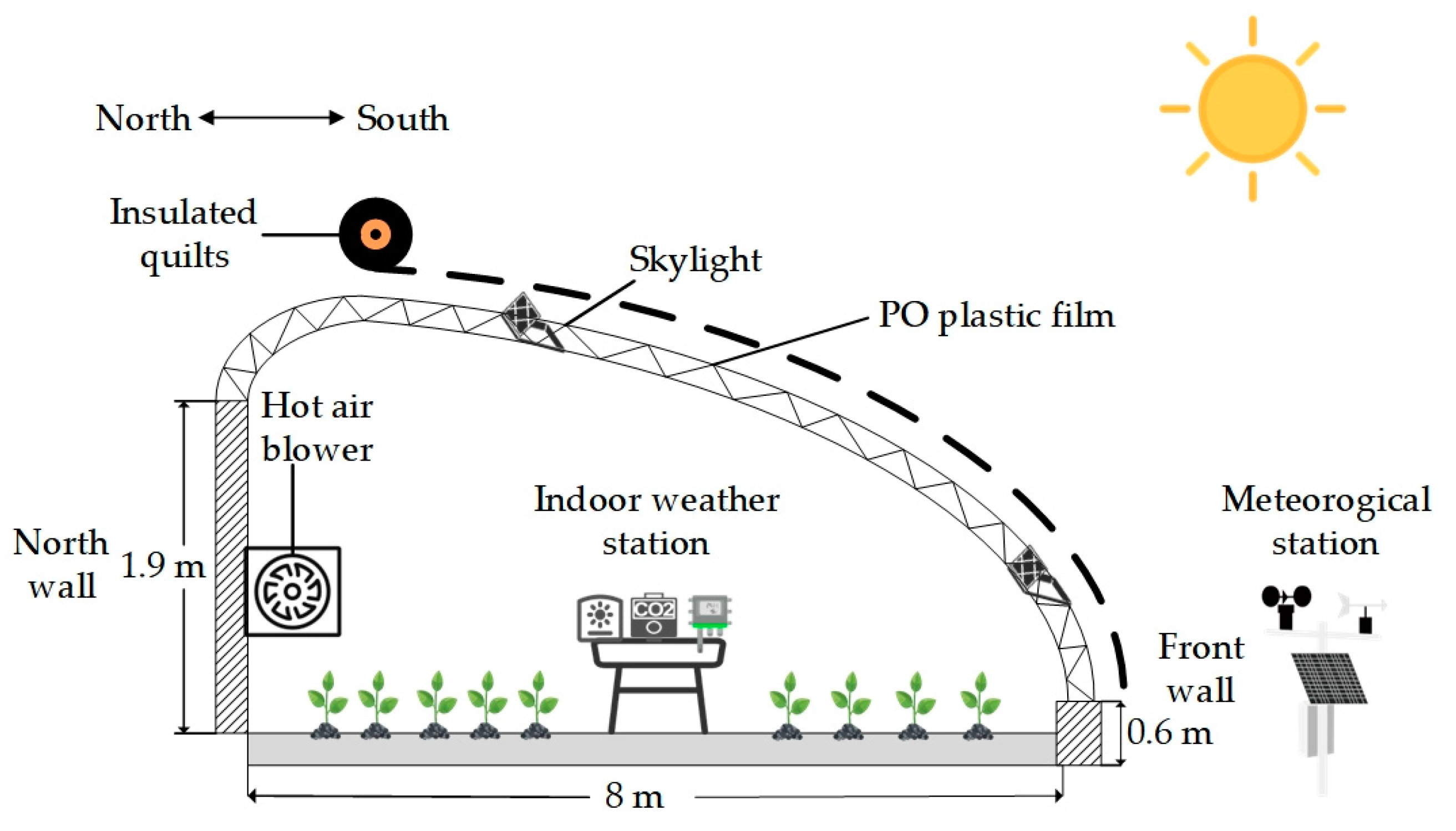
2.1. Experimental Greenhouse

The focus of this experimental study was a prototype sunlight greenhouse located at the Lugang Campus of Xinjiang Agricultural University in Urumqi (43.92° N, 87.35° E). The greenhouse is oriented along a north–south axis, with dimensions of 44 m in length and 8 m in width. Its architectural features include a ridge height of 2.6 m, a back wall height of 1.9 m, and a front wall height of 0.6 m, with no rear slope design. The structure is enclosed on three sides by 240 mm brick-mixed load-bearing walls and is equipped with a lightweight steel frame roof. The roof is covered with a 0.12 mm thick polyethylene olefin (PO) film, which possesses a light transmittance of ≥92%, and an insulating blanket is employed during nighttime. The ventilation system utilizes an opening and closing mechanism with hinged doors, adhering to a winter operational strategy: the front ventilation opening is generally closed, and when the indoor temperature exceeds the set threshold of 30 °C, intermittent ventilation through the roof openings is initiated, with each session not exceeding 30 min. The greenhouse cultivation area was utilized for the planting of tomatoes of the ‘Provence’ variety, employing a two-row planting configuration. The plant spacing was maintained at 0.35 m, with a row spacing of 0.8 m, resulting in a planting density of 3.2 plants per square meter. The average canopy height was recorded at 1.2 m. The structural diagram of the greenhouse is shown in Figure 1.

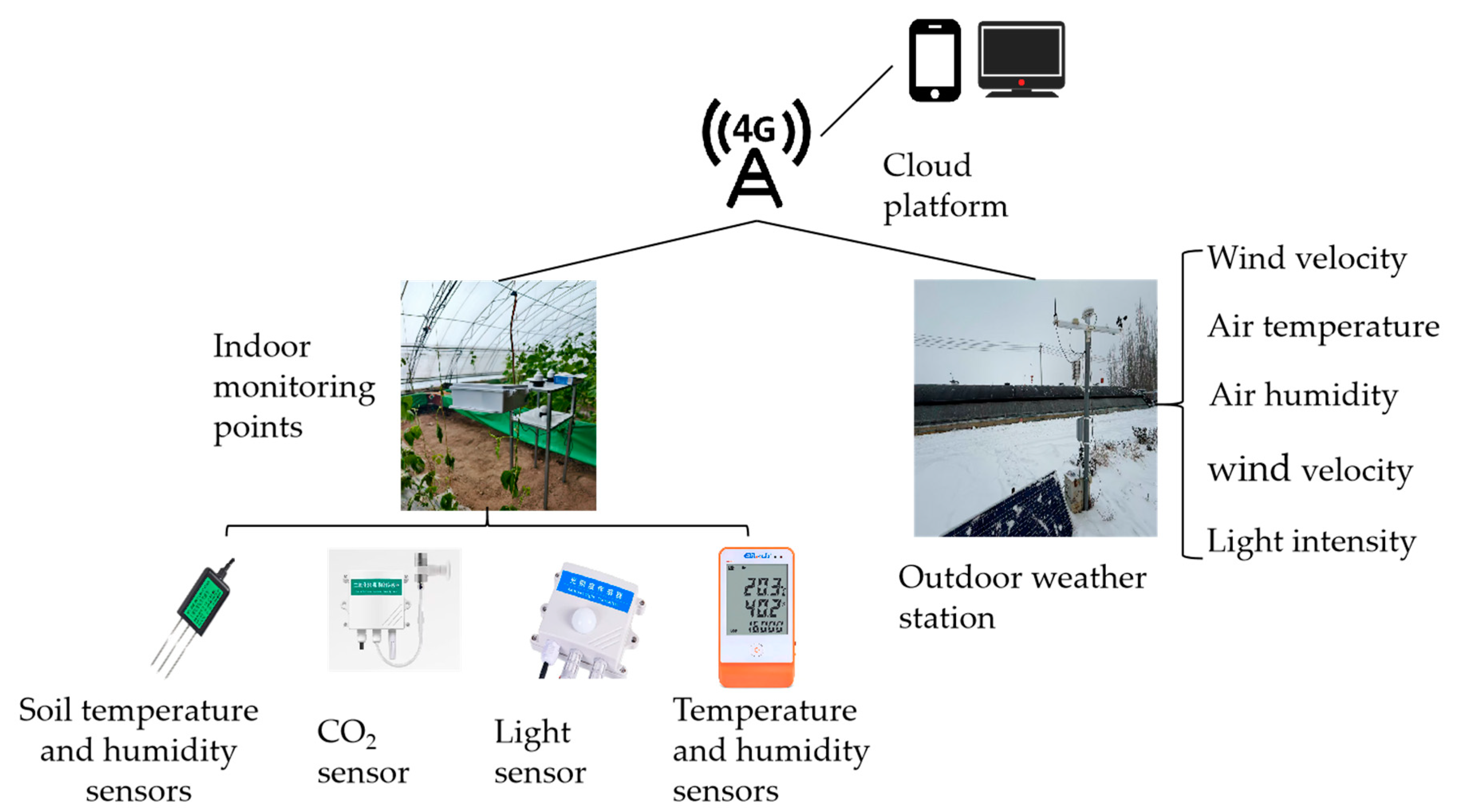
2.2. Data Acquisition Platform

The experimental data collection platform utilized a PH automatic weather station produced by Wuhan Xinhuipu Science and Technology Co., Ltd. in Wuhan, China, by Wuhan Xinhui Science and Technology Co., Ltd. (Wuhan, China) an air temperature and humidity measuring instrument produced by Jingchuang Company in Jiangsu Province, Xuzhou, China. and meteorological instruments produced by Topcloud Agriculture Technology Co., Ltd in Zhejiang Province, Hangzhou, China. The collected parameters included outdoor temperature, outdoor humidity, outdoor illumination, outdoor wind speed, outdoor wind direction, indoor CO₂ concentration, indoor temperature, indoor humidity, indoor illumination, indoor soil moisture, and indoor soil temperature. The structure of the automated monitoring system for greenhouse environmental information is shown in Figure 2, and the specific parameters are listed in

Table 1. Sensor specifications cited.

Instrument	Model Number	Sensor Name	Measuring Range	Accuracy
Outdoor PH automatic weather station	PH-CJ1	Temperature sensor	−50~100 °C	±0.5 °C
		Humidity sensor	0~100% RH	±5%
		Wind speed sensor	0~45 m/s	±0.3 m/s
		Light intensity sensor	0~200,000 lux	±7%
Indoor wireless agricultural detection system	BNL-GPRS-10G	CO2 concentration sensor	0~5000 ppm	±50 ppm
		Soil temperature sensors	−40~80 °C	±0.2 °C
		Light intensity sensor	0~200,000 lx	±1%
Jingchuang temperature and humidity recorder	GSP-6	Temperature sensor	−40~+85 °C	±0.3 °C
		Humidity sensor	10~99% RH	±3% RH

.

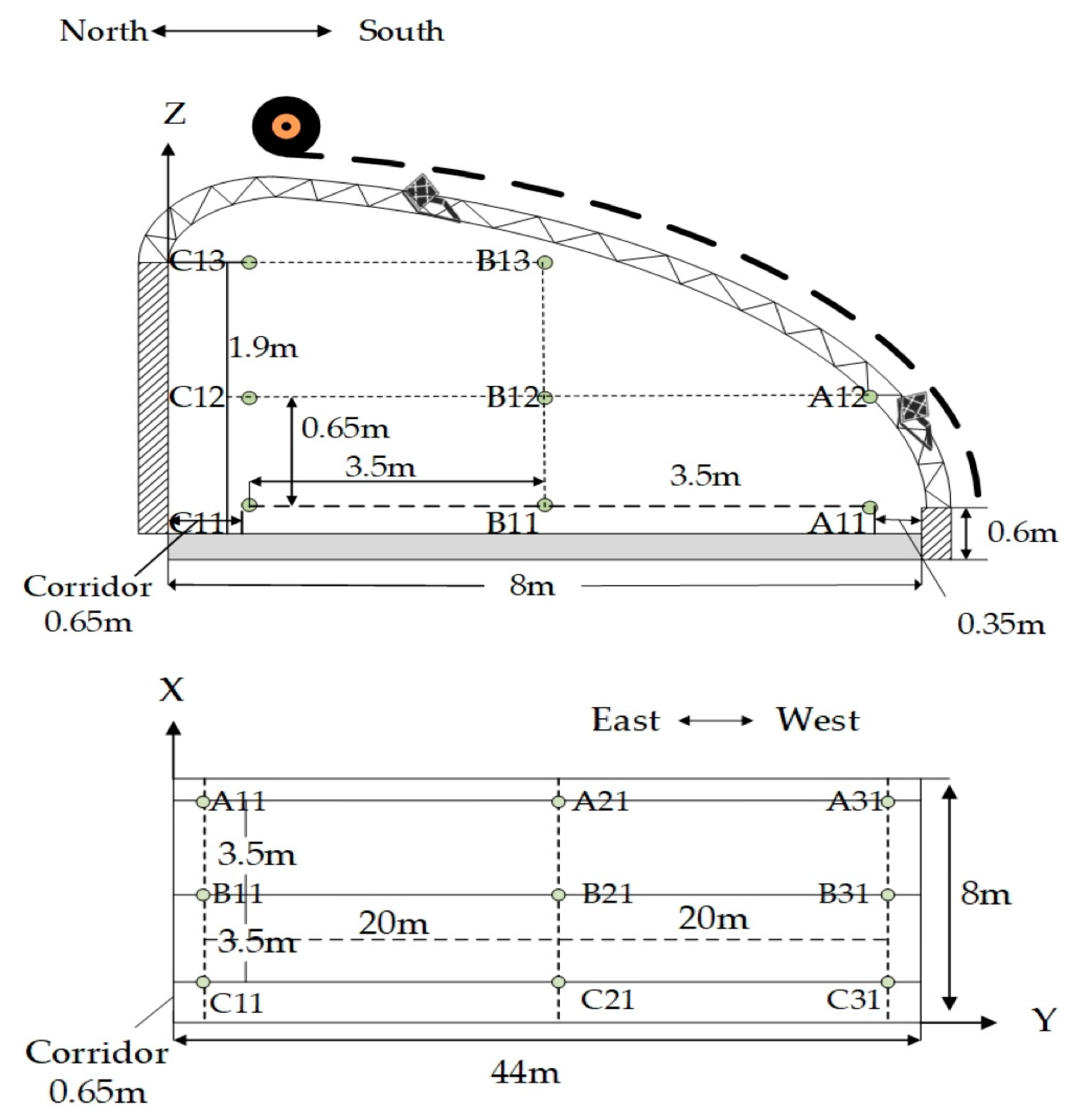
2.3. Greenhouse Temperature Sensor Arrangement

Previous research has demonstrated that the internal temperature of solar greenhouses exhibits considerable spatial heterogeneity, with the precise location of the lowest temperature region during winter being crucial for regulating the greenhouse environment. To thoroughly acquire spatial temperature field data and identify low-temperature extreme points within the greenhouse, this study employs a hierarchical and equidistant deployment strategy. A monitoring grid architecture consisting of 3 columns and 3 rows was designed, deploying a total of 24 temperature sensor nodes. In the specific deployment scheme, the vertical direction was monitored across three layers at intervals of 0.65 m to capture indoor temperature gradient changes, while the horizontal direction adhered to the principle of equidistant distribution (refer to Figure 3 for details). Each node is equipped with Vantech GSP-6 digital temperature sensors produced by Wuhan Jingchuang Technology Co., Ltd. of China which have a measurement accuracy of ±0.3 °C and a sampling interval of 5 min, enabling real-time collection of temperature field data through 4G wireless networking.

2.4. Data Preprocessing and Feature Volume Selection

2.4.1. Data Preprocessing

To eliminate the effects of heterogeneous characteristics in multimodal sensor data, the standard deviation method is used to process abnormal data, and linear interpolation is employed to fill in missing data. All data are normalized using Equation (1) to ensure that their values fall within the range of [0, 1].

$${\mathrm{Y}}^{*}={\displaystyle \frac{\mathrm{Y}-{\mathrm{Y}}_{\min }}{{\mathrm{Y}}_{\max }-{\mathrm{Y}}_{\min }}}$$

(1)

where Y is the original data, and ${\mathrm{Y}}_{\min }$ and ${\mathrm{Y}}_{\max }$ are the minimum and maximum values of the original data after normalization, respectively.

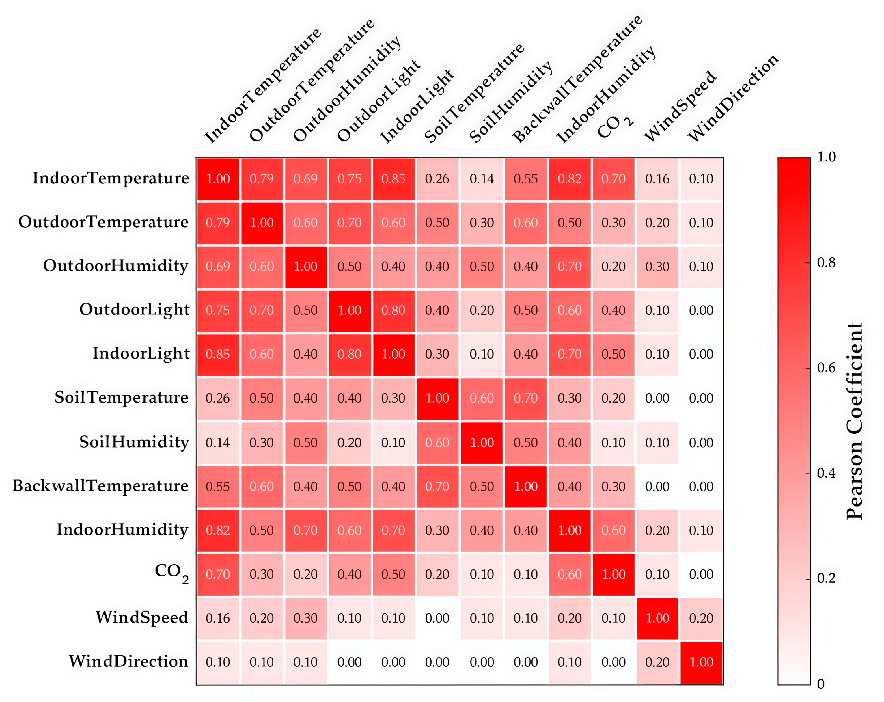
2.4.2. Feature Quantity Selection

In this study, the Spearman correlation coefficient p was used to analyze the degree of influence of each factor on the greenhouse temperature, and the factors with higher correlations were selected as model inputs, with the correlation coefficient p ranging from (−1, 1) and its absolute value tending to be closer to 1, which indicates a stronger correlation. In order to establish the winter greenhouse temperature prediction model, the Pearson correlation coefficients between each environmental factor and the greenhouse internal air temperature were calculated as shown in Figure 4, which showed that the correlation coefficients of indoor air humidity, indoor light, indoor carbon dioxide concentration, outdoor air temperature, outdoor air humidity, and outdoor light intensity were highly correlated with the indoor air temperature. In order to reduce the complexity of the model, other factors were ignored in the modeling.

2.5. Algorithmic Principle

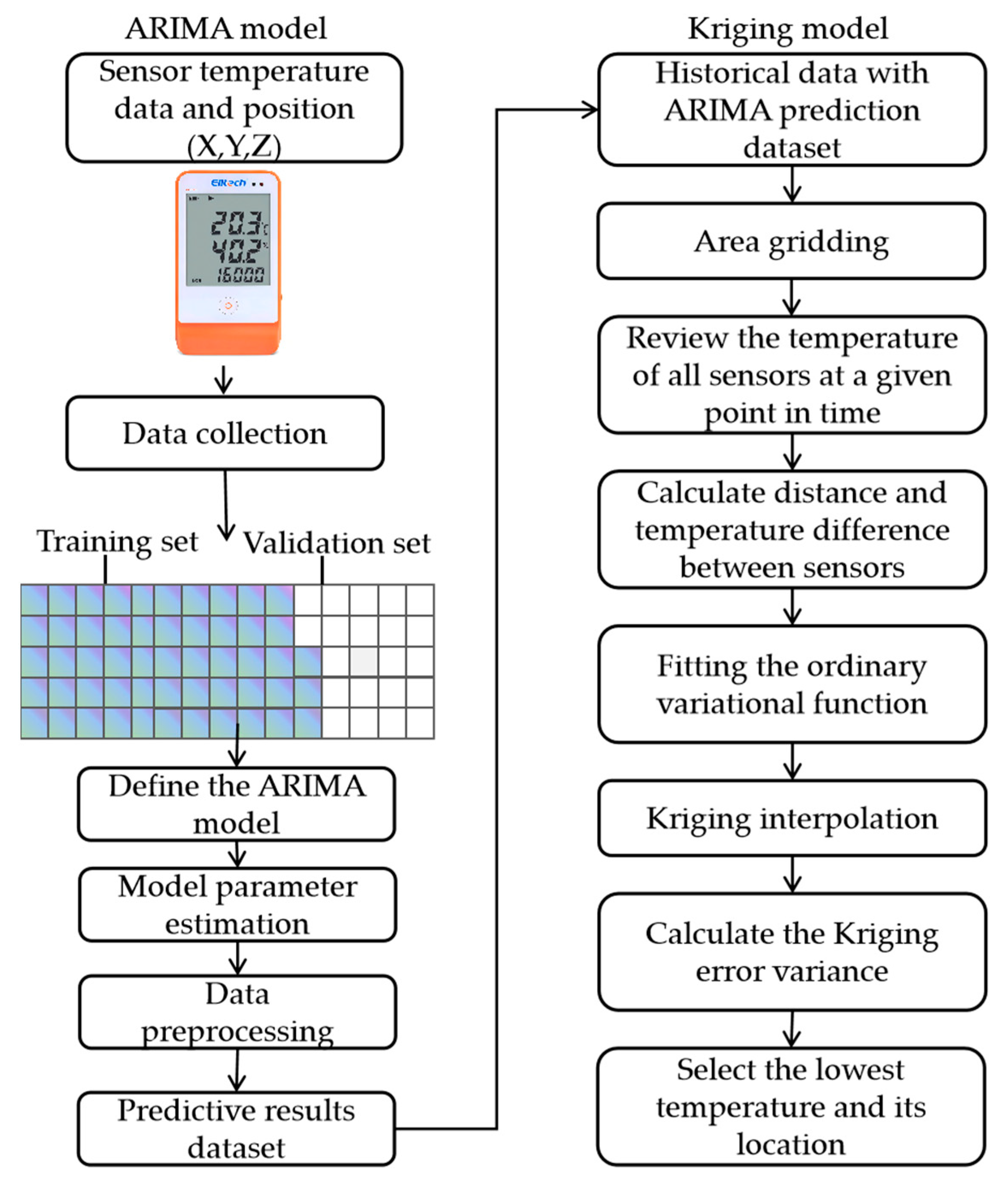
2.5.1. Principle of ARIMA-Kriging Algorithm

The ARIMA-Kriging hybrid model proposed in this study constructs a two-dimensionally coupled modeling framework by integrating time series forecasting and spatial correlation analysis. The algorithm consists of three core parts:

(1)

Time series feature extraction analysis. An autoregressive integral sliding average model (ARIMA) is used to capture the time-domain evolution pattern of temperature data. For any monitoring point s_i, its time series is modeled as follows:

$$(1-\sum _{\mathrm{k}=1}^{\mathrm{p}}{\mathsf{\varphi }}_{\mathrm{k}}{\mathrm{L}}^{\mathrm{k}}\left)\right(1-\mathrm{L}{)}^{\mathrm{d}}\mathrm{Z}({\mathrm{s}}_{\mathrm{i}},\mathrm{t})=(1+\sum _{\mathrm{l}=1}^{\mathrm{q}}{\mathsf{\theta }}_{\mathrm{l}}{\mathrm{L}}^{\mathrm{l}})\mathsf{\epsilon }({\mathrm{s}}_{\mathrm{i}},\mathrm{t})$$

(2)

where L is the lag operator, ${\mathsf{\varphi }}_{\mathrm{k}}$ and ${\mathsf{\theta }}_{\mathrm{l}}$ are the autoregressive and moving average coefficients, respectively, and d is the difference order, which obeys N(0,σ²) distribution.

(2)

Spatiotemporal data fusion. The Kalman filter is introduced to realize the dynamic fusion of predicted values and historical observations.

(3)

Spatial interpolation optimization. A spatially optimal interpolation model based on the ordinary kriging method.

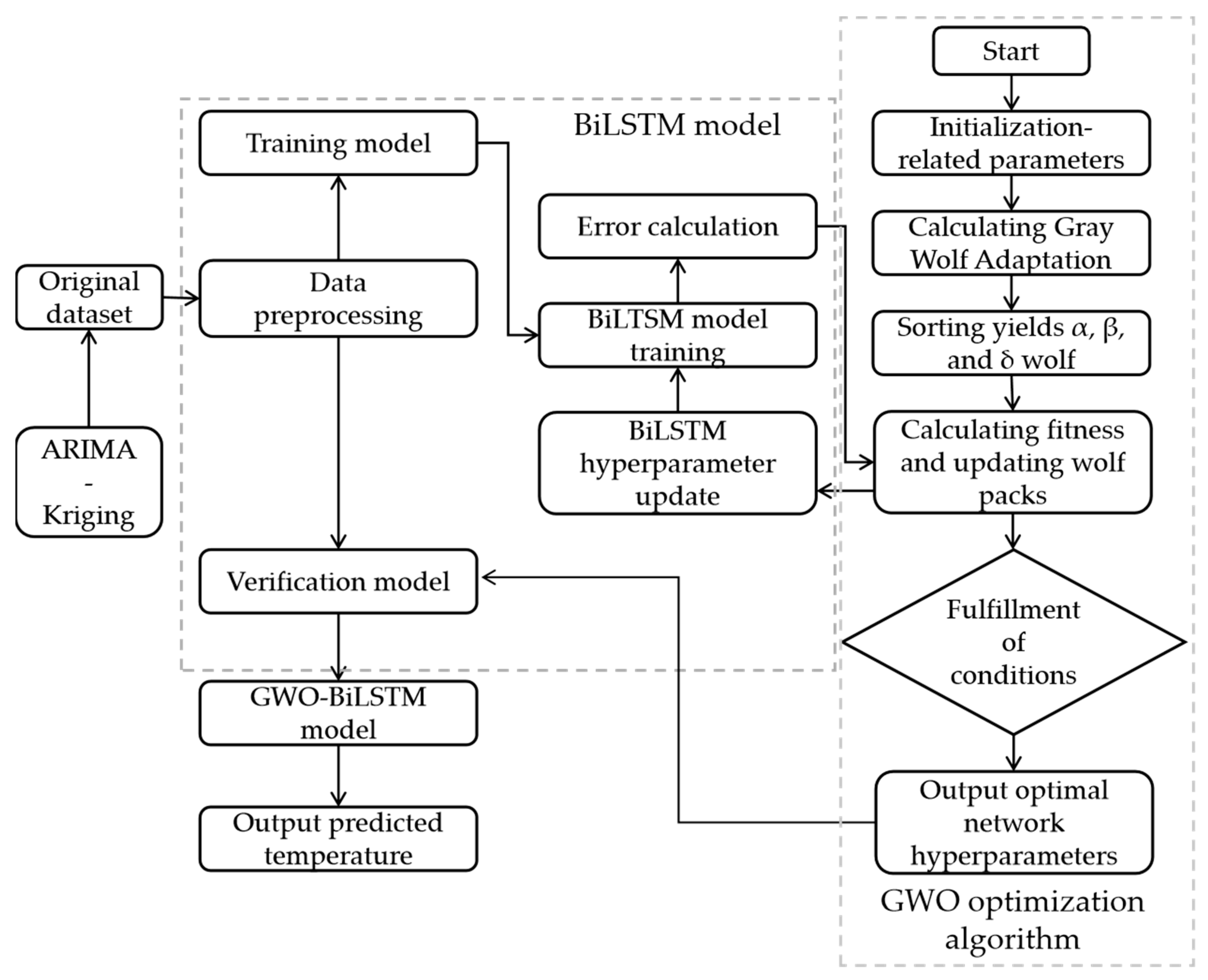
2.5.2. Grey Wolf Optimization Algorithm (GWO)

The training of the BiLSTM model relies heavily on the optimization of parameters. Grey Wolf Optimizer (GWO), a meta-heuristic intelligent optimization search algorithm that mimics the social behavior of wolf packs, can provide good optimization support for BiLSTM. The specific procedure is as follows: Let the grey wolf population P = {Xi|i = 1, …,N}, whose position vector maps the BiLSTM hyperparameter space:

$${\mathrm{X}}_{\mathrm{i}}=[{\mathrm{n}}_{\mathrm{h}},\mathsf{\eta },\mathrm{B},\mathrm{T}{]}^{\top }\in {\mathrm{R}}^4$$

(3)

where n_h is the number of hidden units, η is the learning rate, B is the batch size, and T is the number of iterations.

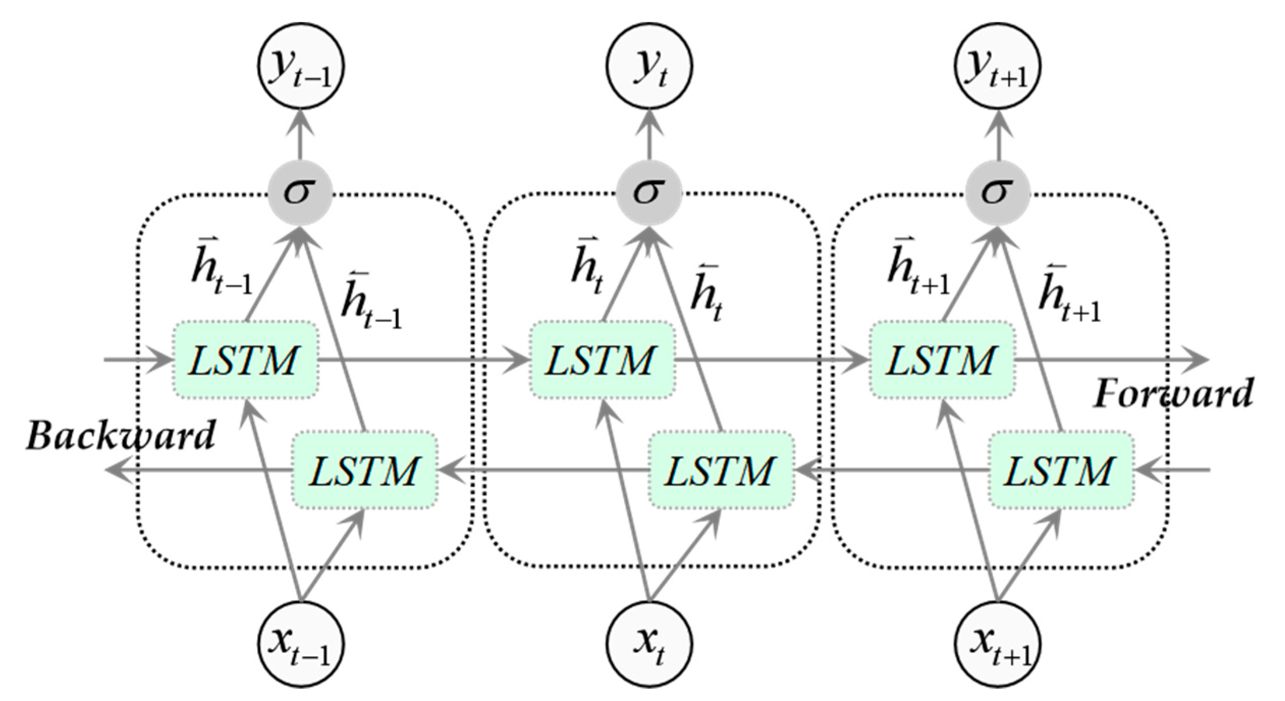
2.5.3. Bidirectional Long Short-Term Memory Network (BiLSTM)

The Bidirectional Long Short-Term Memory (BiLSTM) network is an extension of the traditional Long Short-Term Memory (LSTM) network, as illustrated in Figure 5. It captures the bidirectional dependencies of input sequences by integrating two LSTM networks, namely, the forward and backward passes. Its structure is shown in Figure 6.

The Bidirectional Long Short-Term Memory Network (BiLSTM) consists of two layers of LSTMs: a forward LSTM and a backward LSTM. At each time step t, we compute the output of the forward and backward LSTMs simultaneously, forming the output of the BiLSTM by means of concatenation. Its updated equations are as follows:

$${\overrightarrow{\mathrm{h}}}_{\mathrm{t}}=\mathrm{LSTM}\left({\mathrm{W}}_{\mathrm{f}}[{\mathrm{x}}_{\mathrm{t}}\oplus {\overrightarrow{\mathrm{h}}}_{\mathrm{t}-1}]+{\mathrm{b}}_{\mathrm{f}}\right)$$

(4)

$${\overleftarrow{\mathrm{h}}}_{\mathrm{t}}=\mathrm{LSTM}\left({\mathrm{W}}_{\mathrm{b}}[{\mathrm{x}}_{\mathrm{t}}\oplus {\overleftarrow{\mathrm{h}}}_{\mathrm{t}+1}]+{\mathrm{b}}_{\mathrm{b}}\right)$$

(5)

$${\mathrm{y}}_{\mathrm{t}}=\mathrm{ReLU}\left({\mathrm{W}}_{\mathrm{y}}[{\overrightarrow{\mathrm{h}}}_{\mathrm{t}}\oplus {\overleftarrow{\mathrm{h}}}_{\mathrm{t}}]+{\mathrm{b}}_{\mathrm{y}}\right)$$

(6)

where W_f is the weight matrix of the forward LSTM layer to the output layer; W_b is the weight matrix of the backward LSTM layer to the output layer; and b_f and b_b are the gating bias matrices.

2.6. ARIMA-Kriging Temperature Interpolation Modeling

To mitigate the monitoring bias arising from the spatial heterogeneity of the thermal environment in greenhouses, an ARIMA-Kriging spatiotemporal coupling model was developed (Figure 7). This hybrid model integrates the Autoregressive Integrated Moving Average (ARIMA) model with Kriging interpolation to ascertain the coordinates of the lowest temperature within the greenhouse. The experimental data were obtained from the practical base greenhouse at the Luhong Campus of Xinjiang Agricultural University, which is equipped with 24 Jingchuang GSP-6 temperature and humidity sensors (range: −40 to +85 °C, accuracy: ±0.3 °C) to cover the cultivation area. A total of 124,837 datasets, comprising temperature data and sensor coordinates, were collected from 13 September 2024 to 1 November 2024, with a data acquisition interval of 5 min. Following the Kolmogorov–Smirnov normality test (D = 0.021, p > 0.05), the dataset was divided into a training set (from 13 September to 25 October 2024) and a testing set (from 26 October to 1 November 2024) using a time series blocking method. During the ARIMA modeling phase, the optimal parameter combination was determined through grid search, resulting in an Akaike Information Criterion (AIC = 134.2) and partial autocorrelation function analysis (PACF < 0.05), ultimately leading to the establishment of the ARIMA(2,1,1) forecasting model. By employing a Kalman filter to merge the predicted values with historical observational data, a spatiotemporal feature matrix was constructed as input for ordinary Kriging interpolation. Spatial interpolation was conducted on temperature data for each time point in the greenhouse to reconstruct the temperature field, subsequently identifying the lowest temperature and its coordinates. This process ultimately optimized the layout of temperature monitoring nodes. The model determines the optimal sensor positioning data to be used as input for subsequent predictive models, thereby enhancing the accuracy and efficiency of greenhouse environmental monitoring.

2.7. GWO-BiLSTM Model Construction

Based on the sensor optimization configuration dataset derived from the ARIMA-Kriging model, a temperature prediction model for the greenhouse was developed by integrating an improved Grey Wolf Optimizer (GWO) with a Bidirectional Long Short-Term Memory (BiLSTM) network. As illustrated in the flowchart in Figure 8, the construction of the GWO-BiLSTM-based greenhouse temperature prediction model encompasses the following key stages:

(1) Multimodal data preprocessing. First, the time series data collected by the greenhouse IoT sensing terminal (including temperature and humidity, light intensity, CO₂ concentration, and other sensors) are integrated. The data are preprocessed, including the cleaning of missing values and outliers, as well as the supplementation of missing values and the normalization of data. The processed sample set is divided into a training set (70%) and a test set (30%) according to the principle of time series partitioning to ensure that the time continuity is not destroyed. (2) Multi-strategy co-optimization. Grey Wolf Optimizer (GWO) parameters were initialized using the quasi-oppositional learning strategy (population N = 60) with solution space dimension D = 4 (hidden units, learning rate, batch size, iteration count). BiLSTM hyperparameters were encoded as wolf positional coordinates in GWO’s search space, with the training set used for model adaptation. (3) Multi-objective for optimization. The individual fitness value of the wolf pack is calculated according to the fitness function, and the individual position of the wolf pack is updated. When the search reaches the global optimal position to satisfy the minimum bound or the maximum number of iterations, the network parameters of the optimal BiLSTM are output. (4) Intelligent prediction modeling. The optimized hyperparameters (168 hidden units, learning rate 3.2 × 10⁻³) configured a BiLSTM architecture with input layer (6 tanh-activated BiLSTM cells), attention layer (4-head mechanism), and L2 regularization (λ = 4.7244 × 10⁻⁵). The final model evaluation achieved 2.38 °C MAE on test data, enabling accurate greenhouse temperature predictions.

2.8. Model Evaluation Indicators

To evaluate the performance of the greenhouse temperature prediction model, we selected the root mean square error (RMSE), mean absolute percentage error (MAPE), coefficient of determination (R²), mean square error (MSE), and mean absolute error (MAE) as the primary evaluation metrics. Lower values of RMSE, MSE, and MAPE indicate better model performance. The coefficient of determination (R²) quantifies the goodness of fit between model predictions and observed values, with values approaching 1 denoting optimal predictive accuracy. A lower MAE value corresponds to reduced prediction errors, reflecting enhanced model precision. The comprehensive evaluation of these metrics enables systematic analysis of temporal prediction performance and an objective comparison of model stability across different forecasting horizons. The mathematical formulations for these evaluation metrics are defined in Equations (7)–(11).

$$\mathrm{RMSE}=\sqrt{{\displaystyle \frac{1}{\mathrm{n}}}\sum _{\mathrm{i}=1}^{\mathrm{n}}({\mathrm{y}}_{\mathrm{i}}-{\widehat{\mathrm{y}}}_{\mathrm{i}}{)}^2}$$

(7)

$${\mathrm{R}}^2=1-{\displaystyle \frac{{\sum }_{\mathrm{i}=1}^{\mathrm{n}}({\mathrm{y}}_{\mathrm{i}}-{\widehat{\mathrm{y}}}_{\mathrm{i}}{)}^2}{{\sum }_{\mathrm{i}=1}^{\mathrm{n}}({\mathrm{y}}_{\mathrm{i}}-\stackrel{\mathrm{-}}{\mathrm{y}}{)}^2}}$$

(8)

$$\mathrm{MAPE}={\displaystyle \frac{1}{\mathrm{n}}}\sum _{\mathrm{i}=1}^{\mathrm{n}}\left|{\displaystyle \frac{{\mathrm{y}}_{\mathrm{i}}-{\widehat{\mathrm{y}}}_{\mathrm{i}}}{{\mathrm{y}}_{\mathrm{i}}}}\right|\times 100\%$$

(9)

$$\mathrm{MSE}={\displaystyle \frac{1}{\mathrm{n}}}\sum _{\mathrm{i}=1}^{\mathrm{n}}({\mathrm{y}}_{\mathrm{i}}-{\widehat{\mathrm{y}}}_{\mathrm{i}}{)}^2$$

(10)

$$\mathrm{MAE}={\displaystyle \frac{1}{\mathrm{n}}}\sum _{\mathrm{i}=1}^{\mathrm{n}}|{\mathrm{y}}_{\mathrm{i}}-{\widehat{\mathrm{y}}}_{\mathrm{i}}|$$

(11)

3. Results and Analysis

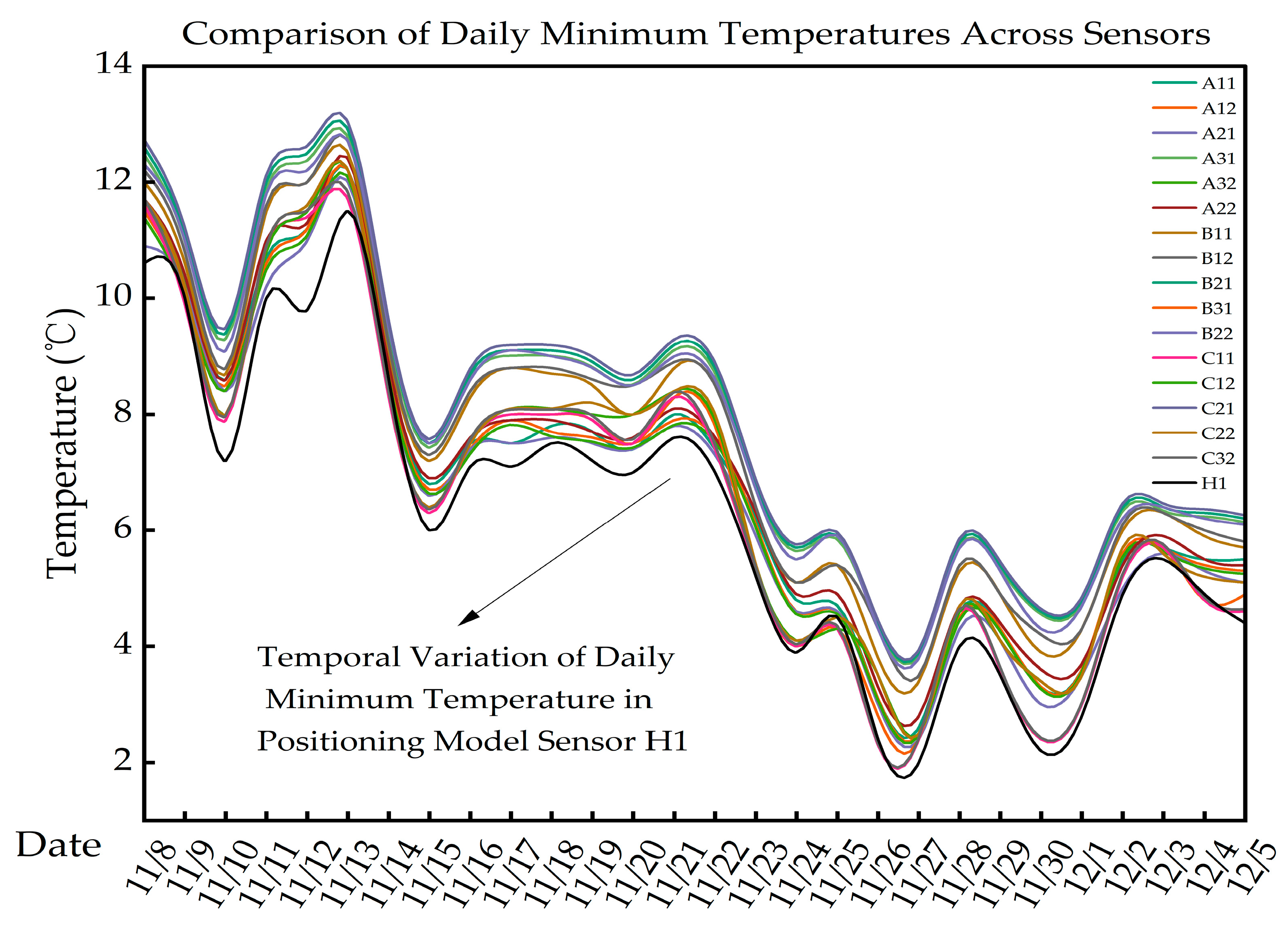
3.1. ARIMA-Kriging Model Validation

This study employs a spatiotemporal coupled ARIMA-Kriging hybrid model to reconstruct the temperature field in a greenhouse. Utilizing a three-dimensional spatial interpolation method (as shown in Figure 9), we successfully analyzed the temperature distribution characteristics at a height of 1.33 m. Quantitative analysis confirmed that this layer, identified as a vertical spatial temperature extreme layer, exhibited a 42% frequency of low-temperature events (T < 8 °C) during the test cycle (Figure 10). The high frequency of low-temperature occurrences was attributed to the thermal inertia characteristics of the greenhouse. Additionally, the use of nighttime insulation cover restricted vertical thermal convection, facilitating the accumulation of cold air within this layer. At the same time, the lowest greenhouse temperature of 7.74 °C was recorded at the coordinate system (X: 7, Y: 0.5, Z: 1.33), and the extreme event occurred on 21 October 2024 at 09:02 (temperature fluctuation ≤ 0.3 °C within the critical time window ± 5 min).

In order to verify the accuracy of the lowest temperature located, we analyzed the temperature monitoring data over a one-month period and selected 16 sensors with different location detection nodes for comparison with the localized location sensor H1. The temperature data of all the sensors are shown in Figure 11. Among the 16 sensors, the statistics showed that the frequency of the lowest temperature appeared in H1 and was reached 23 times, which was significantly higher than that of the other monitoring points. The persistent low temperature observed at the H1 location can be attributed to two primary physical factors. Firstly, its position within the ventilation area at the front end of the greenhouse enhances localized heat dissipation due to the wind outlet effect. Secondly, the north–south axial orientation of the greenhouse results in asymmetric illumination. Specifically, the morning low-angle solar radiation on the eastern side (H1 area) is obstructed by the cotton cover, leading to reduced direct radiation and sensible heat flux. The statistical evidence and analysis of the physical mechanisms corroborate each other, strongly affirming the representativeness of H1 as the point of lowest temperature. This confirmation establishes the accuracy and validity of the localization model and provides a robust foundation for selecting this monitoring point’s time series data for the GWO-BiLSTM model.

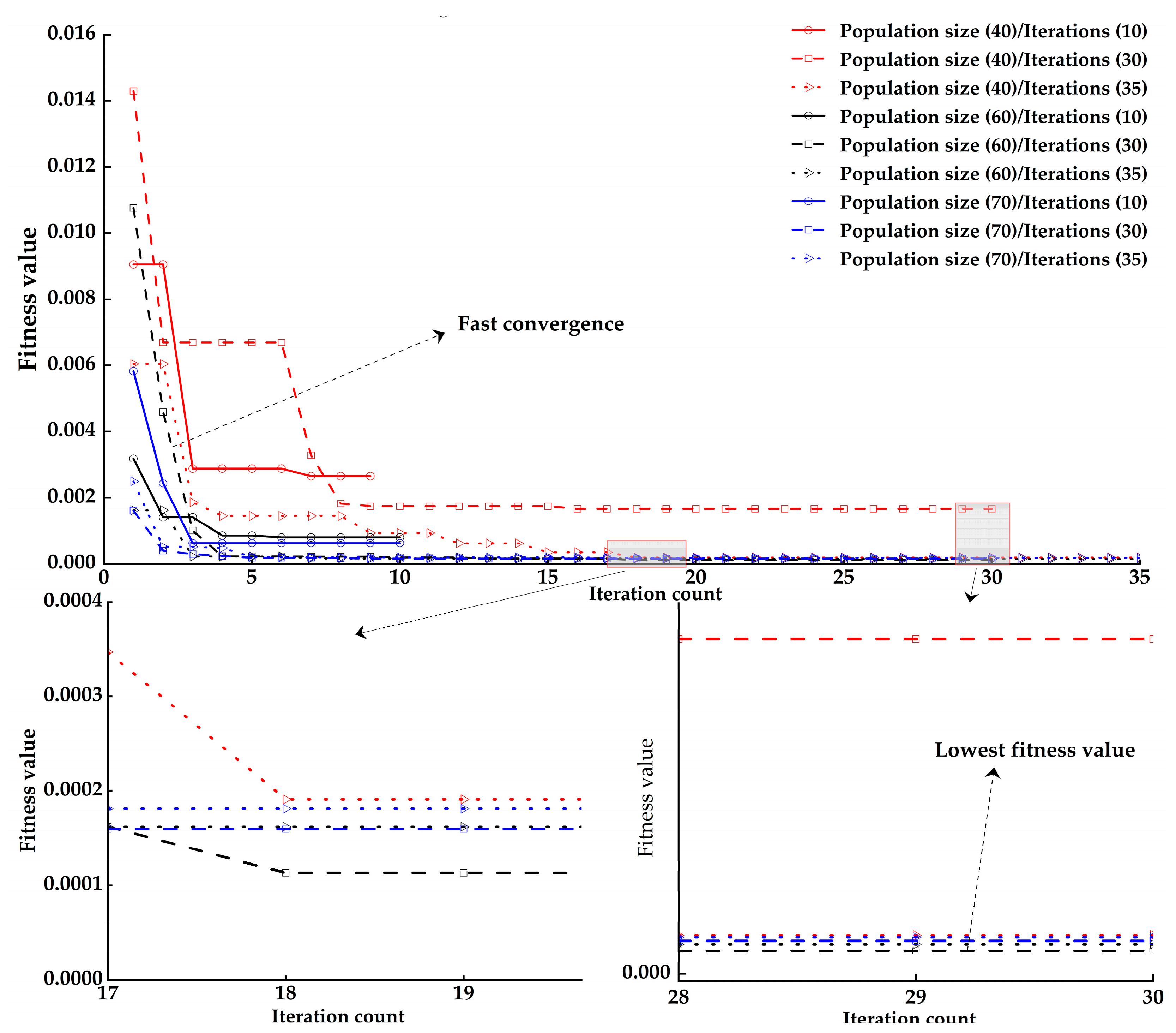
3.2. GWO-BiLSTM Model Parameter Selection

The model is based on the MATLAB 2023b platform, and its deep learning toolbox is utilized for model construction. Referring to the review study of Liu et al. [32] on the Grey Wolf Optimization algorithm, the parameter combinations shown in Figure 12 (population size: 40/60/70; number of iterations: 10/30/35) are evaluated by a grid search system, and the experimental results show that the algorithm converges quickly and reaches the lowest convergence value of 1.13 × 10⁻⁴ when the population size is 60 and the maximum number of iterations is 30. The parameter combination with a population size of 70 (blue curve) has a similar final convergence value, but the need to maintain a larger population size results in an increase in the computational effort for each iteration. With limited computational resources, this leads to longer run times and limited accuracy gains, while too small a number of iterations (<20) makes it difficult to ensure that the parameter space is adequately searched. Therefore, in this study, the population size of the Grey Wolf Optimization algorithm is finally set to 60, the maximum number of iterations is 30, and its hyperparameter optimization range is set as follows: hidden layer neurons [20, 200], maximum training epochs [50, 300], learning rate [1 × 10⁻⁵, 0.1], and L2 regularization [1 × 10⁻⁶, 0.1].

To validate the model performance of the GWO-BiLSTM proposed in this study, standard BiLSTM, LSTM, and PSO-BP were selected for control experiments. The optimal model parameters were obtained by performing GWO training on the pair of BiLSTM models: the number of hidden layer units was 168, the maximum training period was 125, the learning rate was 3.2 × 10⁻³, and the regularization strength was 4.7244 × 10⁻⁵. For the control experiment design, three types of benchmark models were set up to validate the effectiveness of the optimization mechanism: the standard BiLSTM (50 units in the hidden layer), LSTM (single hidden layer), and PSO-BP (Particle Swarm Optimization BP network, corresponding to the settings of 60 particles and 30 iterations). The control group uniformly adopted fixed parameter configurations: learning rate 0.01, training period 100 times, MiniBatchSize 64, and shared the same data preprocessing process and input/output dimensions as the optimized model.

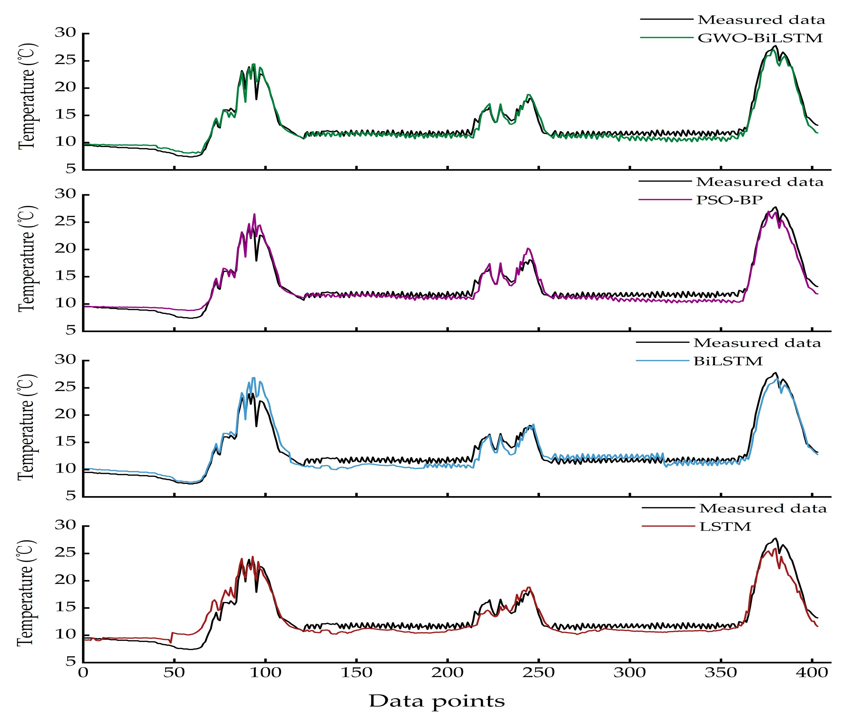
3.3. Multi-Temporal Performance Evaluation and Comparison of Greenhouse Temperature Prediction Models

The prediction of air temperature inside the temperature chamber was carried out for four models, namely, standard BiLSTM, LSTM, PSO-BP, and GWO-BiLSTM, with a prediction step of 10 min. the prediction curves for each model are shown in Figure 13.

In this study, a comprehensive evaluation system integrating the RMSE, MAPE, R², MSE, and MAE metrics was constructed to systematically evaluate the time-series performance of four models, namely, GWO-BiLSTM, BiLSTM, LSTM, and PSO-BP, in greenhouse temperature prediction. As shown in Figure 12, by comparing the predicted values of different models with the measured data, it is found that the prediction errors of the standard BiLSTM, LSTM, and PSO-BP models are relatively large, which are especially significant in the peak, trough, and sawtooth regions where the temperature fluctuates violently.

As shown in

Table 2. Comparison of the prediction performance of four models with different prediction durations (10 min and 30 min).

Model	Forecast Time	Evaluation
		RMSE/°C	MAPE/%	R2	MSE	MAE
GWO-BiLSTM	10 min	0.7889	4.94	0.97	0.63	0.62
	30 min	0.8863	8.5	0.97	0.68	0.65
BiLSTM	10 min	1.1064	6.92	0.93	1.22	0.91
	30 min	1.593	12.8	0.92	1.61	1.21
LSTM	10 min	1.3557	10.8	0.90	1.84	1.07
	30 min	1.8872	10.2	0.90	2.13	1.11
PSO-BP	10 min	0.9467	5.8	0.95	0.90	0.73
	30 min	1.1268	8.6	0.94	1.65	0.89

, the prediction accuracies of all models show a decaying trend when the prediction duration is extended from 10 to 30 min, with the GWO-BiLSTM model exhibiting optimal temporal stability. Specifically, the R² value of this model stays in the narrow fluctuation range of 0.96–0.97, which is significantly better than the fluctuation range of 0.90–0.95 of the other models. In terms of error control, the root-mean-square error (RMSE) of the GWO-BiLSTM model ranges from 0.7889 °C to 0.8863 °C, while the RMSE of the comparison model ranges from 0.9467 °C to 1.8872 °C. Meanwhile, the mean absolute percentage error (MAPE) fluctuations of the GWO-BiLSTM model ranged from 4.94% to 8.5%, which was significantly lower than the MAPE performance of the comparison model from 5.8% to 12.8%. The results showed that the GWO-BiLSTM model performed optimally on all assessment metrics, especially in the 10 min and 30 min prediction intervals, where its R² and MSE metrics were significantly better fitted than those of the other models, with the PSO-BP model performing second best. At the 10 min prediction, the GWO-BiLSTM model had the lowest values of MAPE and RMSE. When the prediction duration was extended to 30 min, the GWO-BiLSTM model was able to maintain the lowest error level despite the increase in prediction errors of all models, which proved its excellent stability and accuracy in prediction tasks at different time scales.

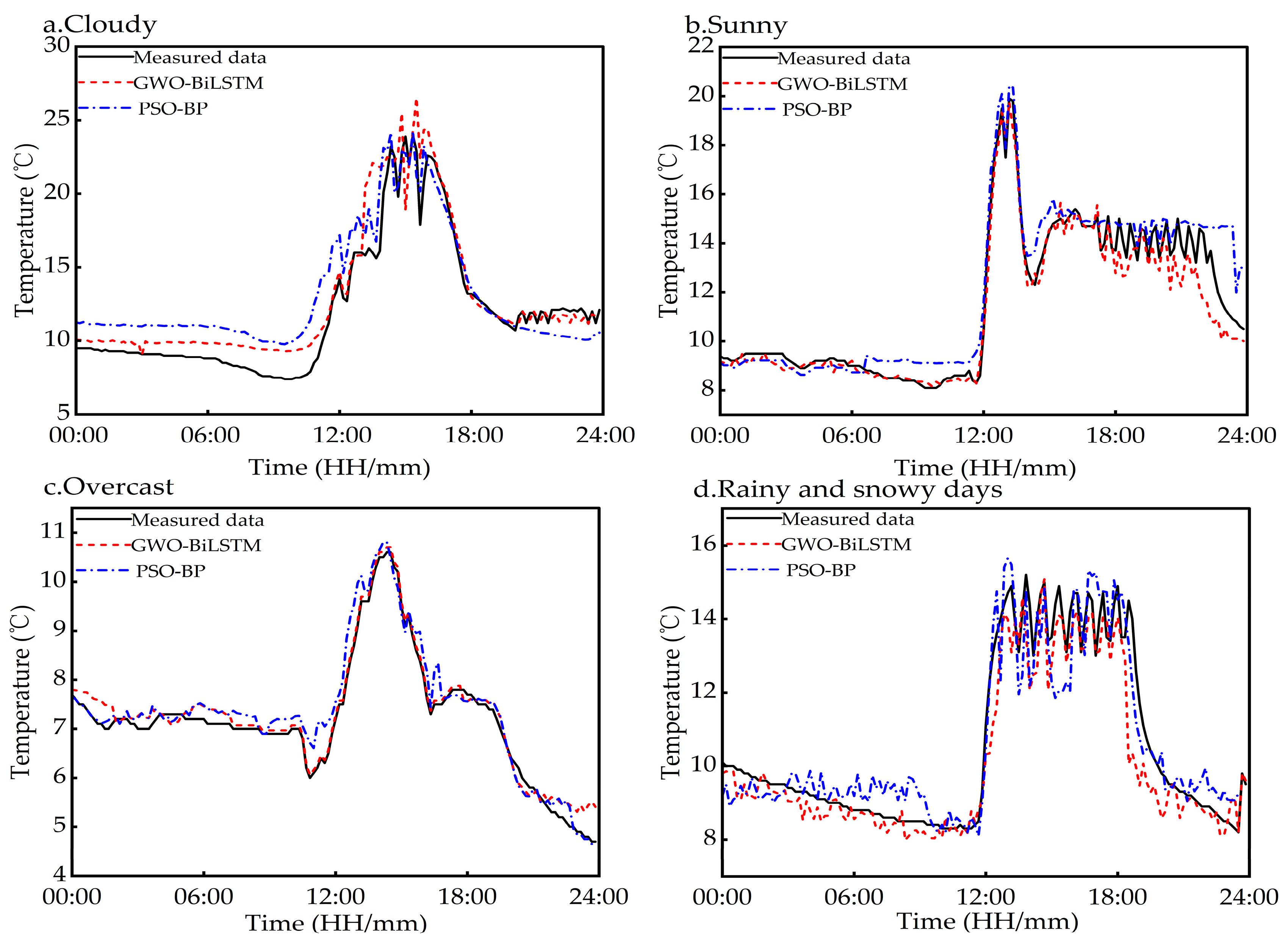
3.4. Comparison of Model Adaptation and Performance Under Different Weather Conditions

To validate the model’s environmental adaptability, a comparative analysis of the predictive performance of the GWO-BiLSTM and PSO-BP models was conducted under four typical weather conditions: cloudy, sunny, overcast, rainy, and snowy days (as depicted in Figure 14).

As shown in Figure 14, the GWO-BiLSTM model exhibits a stronger data fitting ability than the PSO-BP model under all types of weather conditions. As shown in

Table 3. Comparison of the performance of the GWO-BiLSTM and PSO-BP models under different weather types.

Weather	GWO-BiLSTM			PSO-BP
	R2	RMSE/°C	MAPE/%	R2	RMSE/°C	MAPE/%
Cloudy	0.95	1.59	9.8	0.93	2.02	17.49
Sunny	0.97	0.71	3.59	0.96	0.99	7.35
Overcast	0.96	0.86	7.21	0.95	1.1	6.74
Sleet	0.95	0.91	8.53	0.93	1.41	9.93

, under extreme weather (rainy, snowy, and cloudy) conditions, the RMSE values of the GWO-BiLSTM model ranged from 0.91–1.59 °C, which was 35.5–45.3% lower than that of the PSO-BP model, which was 1.41–2.02 °C. At the same time, the improvement in the MAPE metrics of the model reached 42.9–57.3%. Under sunny conditions, the model performance reaches the optimal state, with its R² value as high as 0.97, and the MAPE decreases to 3.59%, which is a 51.2% improvement over the comparison model. Further analysis shows that sudden changes in light intensity (cloudy weather) and sudden changes in humidity (rainy and snowy weather) are the main environmental disturbances that affect the model prediction accuracy. In particular, during cloudy weather, light intensity undergoes significant and irregular fluctuations, resulting in a complex data distribution that increases the model’s prediction error. Conversely, in rainy and snowy conditions, although the humidity changes rapidly, the overall light pattern remains relatively simple, typically characterized by a decrease in light intensity and a stable trend in temperature change. Furthermore, an analysis of the model’s training data revealed that the proportion of rainy, snowy, cloudy, and sunny weather in Urumqi from November to early January 2024 exceeded 90%. This prevalence led the model to predominantly learn these three weather patterns during the training process, thereby resulting in a relatively weak generalization ability in cloudy weather.

3.5. Analysis of Computational Efficiency

In the realm of intelligent transformation of agricultural facilities, the implementation of greenhouse temperature prediction models must prioritize computational efficiency and real-time performance. This section provides a systematic analysis of the computational efficacy of the GWO-BiLSTM model, incorporating hardware configuration experiments and comparative studies to demonstrate its potential application in contemporary agricultural contexts. The training duration of the GWO-BiLSTM model is significantly influenced by the dataset size, model complexity, and computational resource allocation. In this study, utilizing the 2023–2024 fall and winter greenhouse microclimate monitoring dataset, comparative experiments were conducted on heterogeneous hardware platforms: the Intel Core i7-8845h CPU platform required 4.8 h (17,280 s) to complete model training, with a single prediction response time of 0.83 s, whereas the platform equipped with the Intel Core i9-13900h CPU and the NVIDIA GeForce GTX 4080 GPU reduced the training time to 2.1 h (7560 s) and decreased the prediction response time to 0.06 s. The experimental data indicate that the HPC device can decrease the training elapsed time by 58.3%, while its prediction latency fully satisfies the requirements for the real-time regulation of greenhouse environments.

While the GWO-BiLSTM model demonstrates strong performance on high-performance hardware, such hardware may not be accessible in small-scale production environments with limited agro-technical infrastructure. To address this, model simplification can be considered: reducing the number of layers and neurons in the BiLSTM model or decreasing the population size and iterations of the GWO algorithm can lower model complexity and computational demands. To comprehensively assess the computational efficiency of the GWO-BiLSTM model, we conducted a comparison with other models. The LSTM and PSO-BP models, due to their relatively simple structures, exhibit shorter training and prediction times compared to the GWO-BiLSTM model. Nevertheless, the GWO-BiLSTM model offers a notable advantage in prediction accuracy. Consequently, in practical applications, it is necessary to balance prediction accuracy and computational efficiency based on specific requirements.

4. Discussion

Greenhouses serve as essential facilities for off-season agricultural production in northern China, playing a pivotal role in achieving high crop yields. The internal ambient temperature of these structures is a critical factor influencing both crop quality and yield. As a fundamental variable for microclimate monitoring, early warning, modeling, and control, the comprehensive and effective monitoring of greenhouse temperature is of paramount importance. A specific type of greenhouse, which is more sensitive to production costs, necessitates higher sensor input costs and convenient production management. To address the discrepancy between the assumed homogeneity and the actual spatial heterogeneity of traditional greenhouse temperature fields, an ARIMA-Kriging spatiotemporal coupled model is proposed. This model captures temperature dynamics through ARIMA time series decomposition and combines it with Kriging spatial interpolation to reconstruct the three-dimensional temperature field. It identifies the core low-temperature layer (capture frequency 42%) and pinpoints the extreme low-temperature point (coordinates (X: 7, Y: 0.5, Z: 1.33)), thereby reducing sensor costs while providing representative data inputs for modeling.

To accurately regulate the greenhouse environment, we propose the GWO-BiLSTM model, which demonstrates significant advantages in predicting greenhouse temperature. Compared to other models, the GWO-BiLSTM model excels in prediction accuracy and computational efficiency. Specifically, it adeptly captures the highly dynamic trends of light intensity and carbon dioxide concentration, maintaining excellent stability and prediction accuracy in forecasting cyclical changes in greenhouse air temperature. It is noteworthy that the model requires a certain time investment during the initial training phase, as the GWO optimization algorithm is an iterative search algorithm that gradually converges to the optimal solution through multiple iterations. To overcome these limitations, we plan to introduce multiple optimization strategies in future research to reduce the training time while maintaining prediction accuracy.

Throughout this study, we systematically collected greenhouse microclimate datasets for the fall and winter seasons of 2023–2024. Future work aims to further expand the spatial and temporal dimensions of these datasets by supplementing observation data for the spring (March–May) and summer (June–August) seasons. Additionally, we plan to integrate equipment operating parameters, such as roller shutter openness (0–100%) and heating power (0–50 kW), to develop more efficient prediction models and enhance their practicality. The research outcomes are expected to yield significant economic benefits by reducing greenhouse operation costs, providing reliable technical support for intelligent greenhouse control during winter, and preventing frost damage to crops.

5. Conclusions

In this study, we introduce an innovative ARIMA-Kriging-GWO-BiLSTM hybrid model designed for predicting facility temperature and optimizing sensor configuration. The principal conclusions are as follows:

(1)

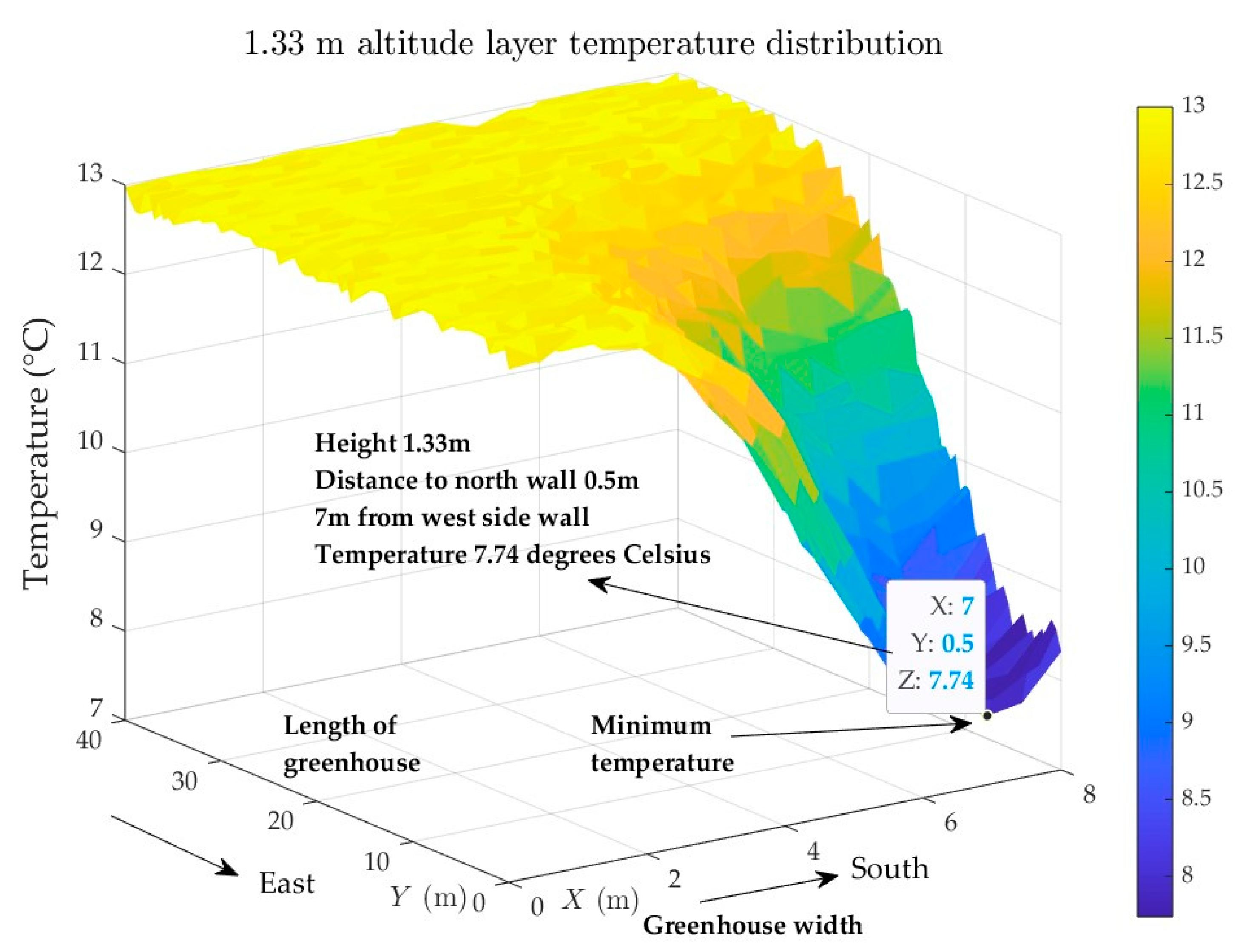
The ARIMA-Kriging model reconstructs greenhouse temperature fields through spatiotemporal data fusion and Kriging interpolation, identifying the vertical 1.33 m layer as a low-temperature core zone and pinpointing an extreme low-temperature point (7.74 °C). Compared with traditional uniform sensor deployment, this approach reduces key monitoring nodes while significantly lowering hardware costs, thereby providing high-value temperature time-series data for subsequent GWO-BiLSTM algorithms.

(2)

The GWO-BiLSTM model is optimized by the Grey Wolf algorithm for Bidirectional Long- and Short-Term Memory networks, and the key indexes are better than those of the three models of BiLSTM, LSTM, and PSO-BP under different prediction steps. Multi-weather validation shows that the model exhibits strong temperature prediction ability under various meteorological conditions, is robust to sudden environmental changes, and can be used for long-term greenhouse air temperature prediction. Further analysis of the lack of sufficient multi-cloud weather data in the training data leads to the relatively weak generalization ability of the models to multi-cloud weather.

(3)

The current study only validated the model in a single sample of greenhouses in Urumqi (43.92° N), and there are still challenges in generalizing the model to other types of greenhouses. The parameters of the ARIMA-Kriging model need to be optimized for different greenhouses to adapt to the differences in their structures and cover materials. In extreme climatic regions, external meteorological fluctuations are more significant in perturbing the heat balance of greenhouses, and the model needs to be further coupled with regional meteorological forecast data as model inputs to enhance the responsiveness to extreme environmental events.

References

1. Hu, J.; Yang, Y.X.; Li, Y.F. Research Status Analysis and Prospects of Greenhouse Environmental Control Methods. Trans. Chin. Soc. Agric. Eng. 2024, 40, 112–128. [Google Scholar]
2. Pi, Y.X.; Zhang, J.S.; Ma, R. Instance Recognition and Model Transfer of Greenhouses Based on Deep Learning. Trans. Chin. Soc. Agric. Eng. 2023, 39, 185–195. [Google Scholar]
3. Fan, L.; Ji, Y.; Wu, G. Research on Temperature Prediction Model in Greenhouse Based on Improved SVR. J. Phys. Conf. Ser. 2021, 1802, 042001. [Google Scholar] [CrossRef]
4. Kavga, A.; Thomopoulos, V.; Pischinas, E.; Tsipianitis, D.; Nikolakopoulos, P. Design and Simulation of a Greenhouse in a Computational Environment (ANSYS/FLUENT) and an Automatic Control System in a LABVIEW Environment. Simul. Model. Pract. Theory 2023, 129, 102837. [Google Scholar] [CrossRef]
5. Li, X.; Zhang, L.; Wang, X.; Liang, B. Forecasting Greenhouse Air and Soil Temperatures: A Multi-Step Time Series Approach Employing Attention-Based LSTM Network. Comput. Electron. Agric. 2024, 217, 108602. [Google Scholar] [CrossRef]
6. Gao, P.; Li, B.; Bai, J.; Lu, M.; Feng, P.; Wu, H.; Hu, J. Method for Optimizing Controlled Conditions of Plant Growth Using U-Chord Curvature. Comput. Electron. Agric. 2021, 185, 106141. [Google Scholar] [CrossRef]
7. Cai, W.; Wei, R.; Xu, L.; Ding, X. A Method for Modeling Greenhouse Temperature Using Gradient Boost Decision Tree. Inf. Process. Agric. 2022, 9, 343–354. [Google Scholar]
8. Jung, D.H.; Kim, H.S.; Jhin, C.; Kim, H.-J.; Park, S.H. Time-Serial Analysis of Deep Neural Network Models for Prediction of Climatic Conditions Inside a Greenhouse. Comput. Electron. Agric. 2020, 173, 105402. [Google Scholar] [CrossRef]
9. Vanthoor, B.H.E. A Model-Based Greenhouse Design Method. Ph.D. Thesis, Wageningen University, Wageningen, The Netherlands, 2011. [Google Scholar]
10. Yang, S.; Liu, X.; Liu, S.; Chen, X.; Cao, Y. Real-Time Temperature Distribution Monitoring in Chinese Solar Greenhouse Using Virtual LAN. Agronomy 2022, 12, 1565. [Google Scholar] [CrossRef]
11. Cheng, X.; Li, D.; Shao, L.; Ren, Z. A Virtual Sensor Simulation System of a Flower Greenhouse Coupled with a New Temperature Microclimate Model Using Three-Dimensional CFD. Comput. Electron. Agric. 2021, 181, 105934. [Google Scholar] [CrossRef]
12. Lee, S.; Lee, I.; Yeo, U.; Kim, R.; Kim, J. Optimal Sensor Placement for Monitoring and Controlling Greenhouse Internal Environments. Biosyst. Eng. 2019, 188, 190–206. [Google Scholar] [CrossRef]
13. Yuan, M.; Zhang, Z.; Li, G.; He, X.; Huang, Z.; Li, Z.; Du, H. Multi-Parameter Prediction of Solar Greenhouse Environment Based on Multi-Source Data Fusion and Deep Learning. Agriculture 2024, 14, 1245. [Google Scholar] [CrossRef]
14. Qin, L.L.; Ma, J.; Huang, Y.M.; Guang, W. Predictive Control of Greenhouse Temperature Hybrid System Based on Accumulated Temperature Theory. Trans. Chin. Soc. Agric. Mach. 2018, 49, 347–355. [Google Scholar]
15. Jia, W.; Wei, Z. Short-Term Prediction Model of Environmental Parameters in Typical Solar Greenhouse Based on Deep Learning Neural Network. Appl. Sci. 2022, 12, 12529. [Google Scholar] [CrossRef]
16. Chen, L.J.; Du, S.F.; Li, J.P.; He, Y.; Liang, M. Online Identification Method for Adaptive Mechanism Model Parameters of Greenhouse Environmental Temperature Prediction. Trans. Chin. Soc. Agric. Eng. 2017, 33, 315–321. [Google Scholar]
17. Chouab, N.; Allouhi, A.; El Maakoul, A.; Kousksou, T.; Saadeddine, S.; Jamil, A. Review on Greenhouse Microclimate and Application: Design Parameters, Thermal Modeling and Simulation, Climate Controlling Technologies. Sol. Energy 2019, 191, 109–137. [Google Scholar] [CrossRef]
18. Zhang, G.S.; Li, T.H.; Hou, J.L. Temperature Prediction Model for Glass Greenhouse Cover Layer Considering Dynamic Absorption Rate. Trans. Chin. Soc. Agric. Eng. 2020, 36, 201–211. [Google Scholar]
19. Xu, K.; Guo, X.; He, J.; Yu, B.; Tan, J.; Guo, Y. A study on temperature spatial distribution of a greenhouse under solar load with considering crop transpiration and optical effects. Energy Convers. Manag. 2022, 254, 115277. [Google Scholar] [CrossRef]
20. Lopez, C.I.; Fitz, R.E.; Salazar, M.R.; Rojano-Aguilar, A.; Kacira, M. Development and Analysis of Dynamical Mathematical Models of Greenhouse Climate: A Review. Eur. J. Hortic. Sci. 2018, 83, 269–279. [Google Scholar] [CrossRef]
21. Chen, Z.; Zhao, H.; Zhang, Y.; Shen, S.; Shen, J.; Liu, Y. State of health estimation for lithium-ion batteries based on temperature prediction and gated recurrent unit neural network. J. Power Sources 2022, 521, 230892. [Google Scholar] [CrossRef]
22. Wang, Y.; Wang, F.; Zhao, Y. Data-driven approaches for greenhouse climate prediction: A review. Comput. Electron. Agric. 2022, 193, 106637. [Google Scholar]
23. Yao, Z.; Lum, Y.; Johnston, A.; Mejia-Mendoza, L.M.; Zhou, X.; Wen, Y.; Aspuru-Guzik, A.; Sargent, E.H.; Seh, Z.W. Machine learning for a sustainable energy future. Nat. Rev. Mater. 2023, 8, 202–215. [Google Scholar] [CrossRef] [PubMed]
24. Ding, J.; Tu, H.; Zang, Z.; Huang, M.; Zhou, S.-J. Precise control and prediction of the greenhouse growth environment of Dendrobium candidum. Comput. Electron. Agric. 2018, 151, 453–459. [Google Scholar] [CrossRef]
25. Wang, H.; Li, L.; Wu, Y.; Meng, F.; Wang, H.; Sigrimis, N.A. Recurrent neural network model for prediction of microclimate in solar greenhouse. IFAC-PapersOnLine 2018, 51, 790–795. [Google Scholar]
26. Qi, P.; Yao, X.; Liu, Q.; Xu, K.; Ren, H.; Xu, K. Prediction of ash melting characteristics temperature for biomass and bituminous coal co-firing based on multiple linear regression model. Agric. Eng. 2024, 40, 174–182. [Google Scholar]
27. Jose, D.M.; Vincent, A.M.; Dwarakish, G.S. Improving multiple model ensemble predictions of daily precipitation and temperature through machine learning techniques. Sci. Rep. 2022, 12, 4678. [Google Scholar] [CrossRef]
28. Grégoire, G.; Fortin, J.; Ebtehaj, I.; Bonakdari, H. Forecasting Pesticide Use on Golf Courses by Integration of Deep Learning and Decision Tree Techniques. Agriculture 2023, 13, 1163. [Google Scholar] [CrossRef]
29. Hoomod, H.K.; Amory, Z.S. Temperature prediction using recurrent neural network for Internet of Things room controlling application. In Proceedings of the 2020 5th International Conference on Communication and Electronics Systems (ICCES), Coimbatore, India, 10–12 June 2020; IEEE: Piscataway, NJ, USA, 2020; pp. 973–978. [Google Scholar]
30. Hao, H.; Yu, F.; Li, Q. Soil temperature prediction using convolutional neural network based on ensemble empirical mode decomposition. IEEE Access 2020, 9, 4084–4096. [Google Scholar] [CrossRef]
31. Zhang, G.; Ding, X.; He, F.; Yin, Y.; Li, T.; Ren, J.; Zhou, J.; Qi, F. Construction of greenhouse air temperature prediction model based on LSTM-AT. Agric. Eng. 2024, 40, 194–201. [Google Scholar]
32. Liu, Y.; As’arry, A.; Hassan, M.K.; Hairuddin, A.A.; Mohamad, H. Review of the grey wolf optimization algorithm: Variants and applications. Neural Comput. Appl. 2024, 36, 2713–2735. [Google Scholar] [CrossRef]
Figure 1. Greenhouse profile.
Agriculture 15 00900 g001
Figure 2. Automatic monitoring system for greenhouse environmental information.
Agriculture 15 00900 g002
Figure 3. Schematic diagram of the spatial arrangement of greenhouse temperature sensors.
Agriculture 15 00900 g003
Figure 4. Correlation coefficient between room temperature and environmental factors.
Agriculture 15 00900 g004
Figure 5. LSTM structure diagram.
Agriculture 15 00900 g005
Figure 6. BiLSTM structure diagram.
Agriculture 15 00900 g006
Figure 7. ARIMA-Kriging model flow.
Agriculture 15 00900 g007
Figure 8. Grey wolf optimization algorithm optimizes the BiLSTM process.
Agriculture 15 00900 g008
Figure 9. Three-dimensional temperature distribution of the 1.33 m height layer in the greenhouse.
Agriculture 15 00900 g009
Figure 10. The probability of low temperatures in the vertical height layer of the greenhouse.
Agriculture 15 00900 g010
Figure 11. (November 8-December 5) Comparison of the daily minimum temperature of the sensor.
Agriculture 15 00900 g011
Figure 12. Comparative convergence curves of populations with varying iteration counts.
Agriculture 15 00900 g012
Figure 13. Comparison curves of predicted and measured values for 4 models.
Agriculture 15 00900 g013
Figure 14. Prediction results of different weather types based on GWO-BiLSTM and PSO-BP models.
Agriculture 15 00900 g014