Abstract
Weeds are an inevitable element in agricultural production, and their significant negative impacts on crop growth make weed detection a crucial task in precision agriculture. The diversity of weed species and the substantial background noise in weed images pose considerable challenges for weed detection. To address these challenges, constructing a high-quality dataset and designing an effective artificial intelligence model are essential solutions. We captured 2002 images containing 10 types of weeds from cotton and corn fields, establishing the CornCottonWeed dataset, which provides rich data support for weed-detection tasks. Based on this dataset, we developed the MKD8 model for weed detection. To enhance the model’s feature extraction capabilities, we designed the CVM and CKN modules, which effectively alleviate the issues of deep-feature information loss and the difficulty in capturing fine-grained features, enabling the model to more accurately distinguish between different weed species. To suppress the interference of background noise, we designed the ASDW module, which combines dynamic convolution and attention mechanisms to further improve the model’s ability to differentiate and detect weeds. Experimental results show that the MKD8 model achieved mAP50 and mAP[50:95] of 88.6% and 78.4%, respectively, on the CornCottonWeed dataset, representing improvements of 9.9% and 8.5% over the baseline model. On the public weed dataset CottoWeedDet12, the mAP50 and mAP[50:95] reached 95.3% and 90.5%, respectively, representing improvements of 1.0% and 1.4% over the baseline model.
1. Introduction
Maize and cotton, as indispensable crops in agricultural production, provide solid support for the textile industry and food security with their high yield and quality characteristics. Weeds, as an inevitable and highly influential factor in the growth of cotton and maize, significantly affect their growth due to the uncertainty of their growth patterns and periods, greatly impacting the yield of cotton and maize [1]. Although the use of herbicides is an effective means of controlling weeds [2,3], the possible negative impacts on the environment and health have increasingly aroused public concern [4]. With the rapid development of artificial intelligence, precision agriculture [5], a related industry in the agricultural field, has emerged. Weed detection, as an important task in precision agriculture, has attracted widespread attention. With the rapid development of computer vision technology, a large number of weed-detection algorithms based on machine learning and deep learning have continuously emerged.
In the early years, some scholars used machine-learning algorithms combined with image features to achieve the purpose of weed detection. Initially, some scholars distinguished crops or weeds by extracting image features such as shape, color, texture, and spectrum. For example, Le et al. [6] used local image texture features through LBP operators and SVM (support vector machines) to distinguish between rapeseed, maize, and radish crops and weeds. Zhu et al. [7] achieved classification of five types of weeds based on image shape and texture parameters through SVM. Tang et al. [8] and Henrik et al. [9] improved the recognition accuracy of crops and weeds by utilizing positional information. Zhang et al. [10] analyzed peas and weeds during the pea seedling period based on color feature distribution and proposed a weed recognition method in complex backgrounds based on R–B color features. Chen et al. [11] proposed a reverse positioning method for weeds in soybean fields based on color features. Wang et al. [12] proposed an accurate weed recognition method based on the SVM model by fusing height features and image features. Although the above models can complete weed recognition, there is a general problem of insufficient feature extraction, resulting in low detection accuracy and poor model stability. In complex environments containing a large amount of noise, using a single feature can no longer achieve accurate detection. Subsequently, some scholars proposed the fusion of multiple features to improve accuracy. Compared with single feature recognition, the fusion recognition method of multiple feature decisions has strong stability and high recognition accuracy. For example, He et al. [13] fused three features of plant leaf shape, texture, and fractal dimension, and proposed a multi-feature fusion weed recognition method combined with SVM and DS (Shafer–Dempster). Sabzi et al. [14] proposed a machine vision prototype based on video processing and metaheuristic classifiers by extracting texture features based on GLCM (gray-level co-occurrence matrix), color features, texture spectral descriptors, moment invariants, and shape features, completing the weed recognition task in potato fields. Deng et al. [15] extracted 101-dimensional features including color, shape, and texture features from weed images, and built three weed classification models of SVM, BP (backpropagation) neural network, and DBN by fusing the above features, improving the classification accuracy of weeds under backgrounds and variable lighting. The above studies provide effective methods and ways for plant recognition and weed detection.
Deep learning has a unique network feature structure, and the features extracted by various deep-learning methods are more effective than manually extracted features. In the field of weed detection, deep-learning methods utilize the differences in spatial and semantic features to achieve the recognition and detection of crops and weeds, effectively improving the accuracy of weed recognition and detection. In recent years, deep-learning models based on CNN (convolutional neural network) architecture have achieved good results in weed classification and detection. In weed-classification tasks, Yu et al. [16] used three DCNN (deep convolutional neural network) models to explore the detection effects of the three models on different types of weeds and concluded that DCNN are very suitable for weed detection in turf grass. Potena et al. [17] used two different CNNs to process RGB and NIR images, completing the rapid and accurate identification of crops and weeds. First, a lightweight CNN was used to segment vegetation, and then another CNN was used to classify crops and weeds. Dyrmann et al. [18] created a CNN network including convolutional layers, pooling layers, and fully connected layers, achieving the recognition of 22 types of weeds, with a classification accuracy rate of 86.2%. Olsen et al. [19] used Inception-v3 and ResNet-50, two CNN models, to perform benchmark performance tests on weed datasets, with classification accuracy rates reaching 95.1% and 95.7%, respectively, and also explained that the ResNet-50 network has good real-time characteristics. In weed-detection tasks, Chen et al. [20] designed the YOLO-sesame model to address the issue of large differences in target size and specifications, using the SE attention mechanism to improve YOLOv4, and completed the recognition task of sesame weeds. The model used the attention mechanism as a logical module, and the improved model had a recognition accuracy of 96.16%. Zhang et al. [10,21] also made some improvements based on YOLO v4 to meet the requirements of weed detection. Fan et al. [22] started from the high similarity between weeds and crops and the multi-scale of weeds, and improved the faster R-CNN network by using attention mechanisms, BiFPN, and bilinear interpolation methods, completing the weed-detection task in corn fields, with the model’s recognition accuracy reaching 97.42%, and the reasoning speed becoming better than the original model. Ahmad et al. [23] used VGG16, ResNet50, InceptionV3, and YOLO v3 to classify and detect common multiple types of weeds in corn and soybean fields for two tasks. In the classification task, the VGG16 model performed the best, with an accuracy rate of 98.90% and an F1 score of 99%. In the detection task, the mAP total score was 54.3%. Fan et al. [24] improved the YOLOv5 network by using attention mechanisms, BiFPN structure, and shuffleNet v2 backbone for weeds in non-structured environments, completing the weed recognition task in apple fields. Compared with traditional machine learning, deep-learning models often show better results, but this method relies on a large amount of data for training. The existing weed datasets do not seem to be as perfect as imagined, and the high similarity between weeds and crops, the small scale of weeds, and other issues also pose high requirements for weed-detection models.
Based on the above issues, we first collected 2002 weed images, and selected 1651 of them to build a weed dataset, solving the problem of data sources for model training. Secondly, for deep-learning models, the YOLO (you only look once) series, as a rapidly evolving one-stage real-time detector, has gained widespread attention for its high detection accuracy. Therefore, we chose the current mainstream YOLOv8 [25] as our baseline model and designed the MKD8 model specifically for weed-detection tasks.
The main contributions of this paper are:
- We constructed the CornCottonWeed weed dataset from the Xinjiang region, containing 1651 images and 1953 annotated bounding boxes, which are used for weed-detection tasks.
- In order to solve the problems of weed category misjudgment and instance misidentification (for example, identifying crops as weeds) caused by the large variety of weeds and the small appearance difference between crops and weeds, we designed the CVM and CKN modules. The CVM module focuses on capturing deep features, providing the model with rich deep-feature representation while also facilitating feature transfer. The CKN module captures fine-grained semantic features between instances to better distinguish instances, thereby improving the model’s discriminative ability.
- In order to solve the problem of missed detection of weed images due to background noise interference, we designed the ASDW module to suppress background noise through dynamic convolution and attention mechanism, thereby enhancing the model’s ability to locate and detect weeds.
- The MKD8 model significantly improves detection accuracy on both the CornCottonWeed dataset and the public CottoWeedDet12 dataset, providing a novel solution for weed-detection tasks and greatly advancing the development of precision agriculture.
2. Materials
2.1. Data Acquisition
Aiming at the shortage of current weed datasets and the different quality of available datasets, we used intelligent electronic equipment to capture 2002 weed images with the main resolutions of (4096, 3072) and (2736, 3648), and then constructed the CornCottonWeed weed dataset. The data were taken in July and August 2023 in the cotton and corn fields of Huaxing Farm in Xinjiang, China. Weed species include White_Amaranth, Barnyard_Grass, Day_Lily, Portulaca_Oleracea, Dogwood, Gray_Quinoa, Chenopodium_Album, Reeds, Camel_Thorn, and Chinese_Ixeris_Denticulata, a total of 10 types of weeds. In order to ensure the quality and diversity of the data, we selected the background with typical farm characteristics (such as soil, film, etc.), and adopted the method of multi-angle shooting. In addition, in order to minimize the impact of light changes on image capture, we mainly shoot between 7 a.m. and 7 p.m. on sunny and cloudy days.
2.2. Data Annotation
To ensure the quality of the image dataset, we conducted a rigorous manual screening process for the collected images. The selection criteria included the number of weed instances in the images, the clarity of the images, and the severity of background noise. We ultimately retained 1561 high-quality image instances. Subsequently, we adopted manual annotation methods to provide detailed labeling for these images. To ensure the accuracy of the annotations, we learned professional annotation skills and used the Labelimg tool for the dataset annotation work. Professional annotation can use small rectangular boxes to accurately label weed instances in the images, thereby enhancing the overall quality of the dataset. Using the Labelimg tool not only improved the efficiency of annotation but also ensured that the annotation information format matched the .txt format required for YOLO model training. In this way, we were able to directly obtain key information such as the center coordinates, height, and width of the image instances, all of which were stored in .txt format.
2.3. CornCottonWeed Dataset Analysis and Data Augmentation
As shown in Figure 1, we present representative annotated images of various weeds in the dataset, where the category name of the weeds in each row is labeled on the far left, and the weed instances in the images are annotated with red bounding boxes. As depicted in Figure 2a, we show the number of images contained in each category of the dataset and the distribution of all instances’ locations within the original images. To alleviate the issue of dataset sample imbalance and to increase data diversity, we employed data augmentation, as shown in Figure 3. Specifically, we applied random transformations (such as flipping, cropping, rotation, scaling, color adjustment, translation, etc.) and sample stitching to the original sample images, generating a large number of new samples with different viewpoints, sizes, lighting conditions, and backgrounds.
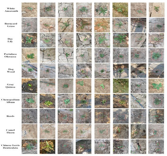
Figure 1.
Sample weed images from the CornCottonWeed dataset.
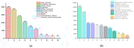
Figure 2.
(a) The number of images in the CornCottonWeed dataset. (b) The number of images in the CottoweedDetl2 dataset.
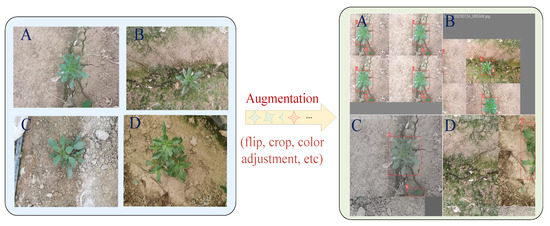
Figure 3.
Data augmentation techniques involved in the experiment. The graph on the left is the original image, and the graph on the right is the image after data enhancement. Images (A–D) in the two pairs of pictures are one-to-one correspondence.
3. Method
3.1. Overview
The MKD8 model first enhances the model’s ability to extract deep and fine-grained features through the CVM module in the backbone and the CKN module in the neck. Then, the ASDW module is employed to suppress the interference of background noise, thereby improving the model’s ability to localize and detect weed instances. The structure of the MKD8 model is shown in Figure 4.
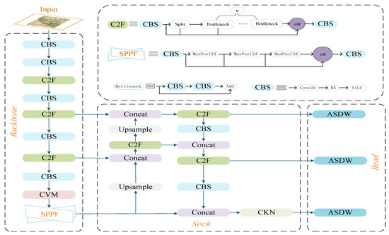
Figure 4.
Overall Structure of the MKD8 Model Diagram.
3.2. CVM Model
As network depth increases, traditional C2F modules cannot effectively retain deep-feature information (details and important information of the original input data), resulting in model performance degradation. Inspired by Liu et al. [26], we designed the CVM module to alleviate the above problems. First, through the long sequence global modeling method of the SS2D module, deep features are retained to the maximum extent. Secondly, in order to improve the model’s utilization of deep global features, we also use regularization technology and use drop path to randomly discard branch paths, so that the model cannot overly rely on certain specific paths. At the same time, this also improves the generalization ability of the model to a certain extent. The structure diagram of CVM is shown in Figure 5.
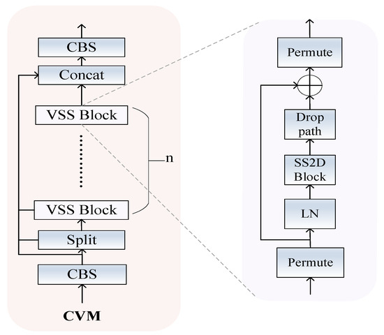
Figure 5.
The CVM model diagram.
Specifically, the workflow of the CVM module is as follows. First, the input is processed through the convolution module, which consists of 1 × 1 convolution, batch normalization, and SiLU activation function. The output is then split into two parts: one part is fed into the VSS block for deep-feature extraction via SS2D and drop path, while the other part is kept via skip connections to preserve feature information. Finally, the concatenated features are passed through another convolutional module to produce the output of the CVM.
3.3. CKN Model
In the field of weed detection, due to the strong appearance similarity between some weeds and between weeds and crops, the model has problems such as incorrect weed category judgment and mutual misjudgment of weeds and crops. Therefore, whether the fine-grained semantic features of the instance can be fully captured plays a decisive role in weed detection. The weak appearance difference between instances in weed images makes it difficult for traditional two-dimensional convolution to capture fine-grained semantic features, which reduces the performance of the model. However, we know that the activation function can map data from nonlinear space to linear space, so that features can be better identified and classified. Therefore, the selection of activation function is very important for the model to understand image features, especially fine-grained features.
We noticed that the edge of the KAN network (formula as follows) uses a learnable activation function [27].
where x is input, function replaces the B-spline function, and is the output of the Kan convolution.
Unlike ordinary two-dimensional convolutions that use fixed activation functions, the learnable activation function allows the model to adaptively activate the captured features, realize further characterization, and enable the model to better focus on the fine-grained differences of different features.
Inspired by Drokin, Tawan et al., we designed the CKN module. First, we use the KAGN_C convolution based on the Kan network to replace the convolution module in the bottleneck module, [28], so that the activation function in the convolution has learnable characteristics, thereby better capturing fine-grained semantic features. Secondly, unlike the B-spline function in the Kan network, we use the Gram polynomial as the spline function of the KAGN_C convolution, because the discreteness of the Gram polynomial can better process image data [29]. Finally, the new bottleneck module is embedded in the C2F module to form the CKN module.
Specifically, the workflows of CKN and CVM are basically the same, the difference lies in the way of processing features. KAGN_C focuses on semantic features, and the learnable activation function makes the representation of fine-grained semantic features more complete, improving the model’s ability to distinguish instance categories (Figure 6).
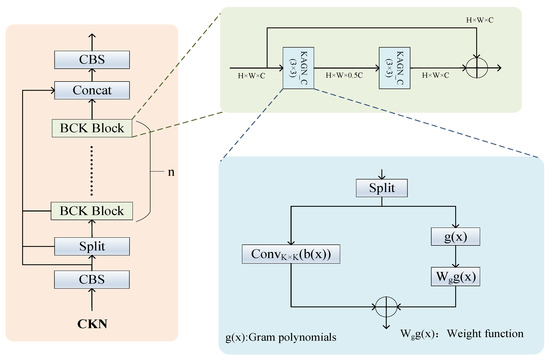
Figure 6.
The CKN model diagram.
3.4. Adaptive Sampling Dynamic Weighting Model
We found that images in weed datasets typically contain a large amount of background noise, which poses a high demand on the model’s detection capabilities. Through research on the head part of YOLOv8, we discovered that although YOLOv8 decouples the detection head, significantly improving the model’s convergence speed by separating classification and regression into two detection branches, it is limited by its reliance on single feature maps for classification and regression predictions. This limitation hinders the detection head’s ability to capture multi-scale feature fusion, reducing detection performance. Based on the anchor-free detection strategy, the model directly predicts the center coordinates of the target, making the localization of small targets difficult and limiting the model’s ability to detect weeds. Inspired by DyHead [30] applied attention mechanism, we designed the ASDW (adaptive sampling dynamic weighting) module, as shown in Figure 7.
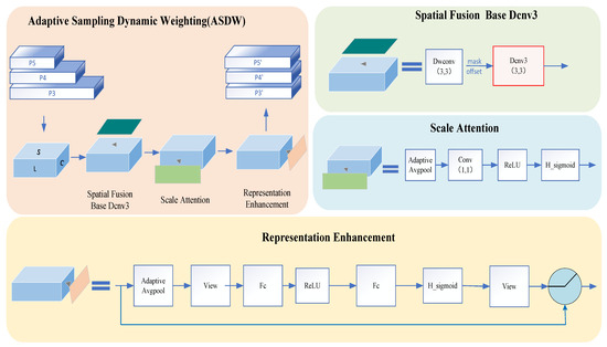
Figure 7.
The adaptive sampling dynamic weighting (ASDW) model diagram.
Specifically, we selected three scales of features from the P3 (large), P4 (medium), and P5 (small) parts of the model’s neck section. In the spatial fusion base Dcnv3 [31] module, we use DWconv convolution to obtain spatial information: offset and mask for each feature map. Thanks to Dcnv3’s ability to dynamically adjust the sampling position of the convolutional kernel for weighting, we enhanced the spatial features by combining the three feature maps with their respective spatial information using Dcnv3. Then, for the feature maps from P3 and P5, we used downsampling and bilinear interpolation to normalize the large and small scale feature maps. Then, for each feature map, we used the scale attention module to enhance the semantic features based on their semantic importance. After that, we adopted the following fusion strategy: P3 and P4 are fused to get a new P3; P5 and P4 are fused into a new P5. Finally, we used DyReLU [32] to implement the representation enhancement module, mapping the pooled features through two fully connected layers, and dynamically activating parameters to weight and fuse the outputs of each branch. This enables the model to adapt to different input features more flexibly, enhances the model’s nonlinear expression ability and feature selection capabilities, and thereby suppresses the interference of background noise on the model.
4. Results and Discussion
4.1. Dataset Selection
In terms of selecting the experimental dataset, we initially chose the CornCottonWeed dataset, for which detailed information has already been provided in the Materials and Methods section of this paper, so I will not repeat it here. Additionally, we selected the CottoWeedDet12 [33] dataset, which is currently considered the highest quality dataset for weed-detection tasks. The CottoWeed12 dataset was collected from cotton fields at the research farm of Mississippi State University. The weed information included in this dataset is shown in Figure 2b. The dataset’s labeling was carried out not only by trained personnel but also inspected by experts in the field of weed science, ensuring a high quality of label annotation. Using this dataset can better reflect the effectiveness of the MKD8 model.
In terms of dataset division, we adopted a random division strategy and performed proportional sampling according to categories to ensure the consistency of sample distribution during dataset division. For the two datasets, we designed two different schemes. For the CottoWeed12 dataset, characterized by an ample sample size and relatively balanced class distribution, we adopted a 7:2:1 ratio to allocate a substantial proportion to the training set, thereby facilitating effective model training while maintaining adequate validation and test sets for comprehensive model evaluation.In contrast, the CornCottonWeed dataset exhibits a relatively limited sample size and noticeable class distribution differences. Therefore, we employed a 6:2:2 ratio to preserve a higher proportion of samples in both the validation and test sets, aiming to enhance the robustness and generalization capability of the model evaluation. We show the information of each category in the divided dataset in the Appendix C.
4.2. Experimental Setup
We conducted our experiments on an NVIDIA A40 GPU. During the model training process, we specified the initial learning rate, final learning rate, gradient descent momentum, weight decay coefficient, gradient descent algorithm, and training epoch parameters. In addition, to enhance training speed and reduce computational resource consumption, we employed AMP (automatic mixed precision) training. Since we set the number of epochs to 300, to mitigate the risk of overfitting, we used the patience parameter to implement an early stopping mechanism, with 50 being the threshold for this mechanism. The detailed configuration parameters of the experiment are shown in Table 1 and Table 2.

Table 1.
Platform settings.
Table 2.
Parameter settings.
4.3. Evaluation Metrics
To evaluate the model and its detection performance, we employed several metrics, including mAP, P (precision), R (recall), FPS, Params (parameters), and GFLOPs. Among these metrics, mAP represents the average precision across all categories. P denotes the accuracy of object detection, reflecting the proportion of correctly identified detections. R indicates the proportion of actual positive samples that are correctly predicted. FPS measures the number of image frames the model can process per second. Params represents the model’s complexity and storage overhead. GFLOPs, as a measure of computational complexity, indicates the number of floating-point operations performed per second. The higher the GFLOPs, the greater the computational load, and the slower the inference speed.
P and R primarily focus on the accuracy and completeness of the model, respectively, while mAP comprehensively reflects the overall model performance. Meanwhile, FPS, Params, and GFLOPs are associated with the model’s complexity and computational efficiency. To evaluate the model’s detection performance, we specifically focus on mAP50 (IoU = 0.50) and mAP[50:95] (IoU = [0.50:0.95]), with P and R considered as secondary factors. Regarding the model itself, we emphasize the values of FPS, Params, and GFLOPs.
4.4. Comparison Experiments
In this experiment, we used the following models: one-stage models including the YOLO series—YOLOv3 [34], YOLOv3u [34],YOLOv5 [35], YOLOv6 [36], YOLOv7 [37], YOLOv8 [25], YOLOv9 [38], and YOLOv10 [39]. Transformer-based models included RT-Detr-l [40], RT-Detr-R-50 [40], and RT-Detr-R-101 [40]. For two-stage models, we chose the well-known Faster-R-CNN [41]. The experimental results are shown in Table 3, Table 4 and Table 5 and Figure 8.
Table 3.
Experimental results of different models on the CornCottonWeed dataset. Black bold font is the best effect.
Table 4.
Experimental results of different models on the CottoWeed12 dataset. Black bold font is the best effect.
Table 5.
Model parameters, FPS, and computational complexity. Black bold font is the best effect.
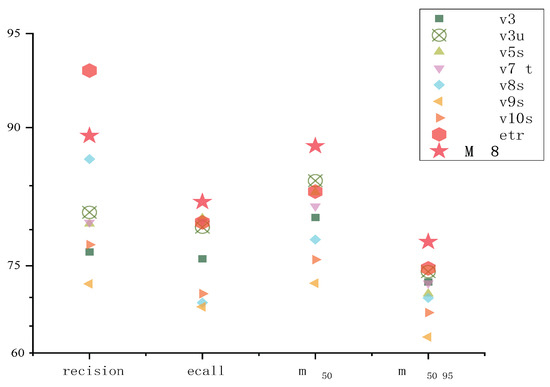
Figure 8.
The experimental results visualized for the CornCottonWeed dataset.
Model Analysis: In terms of detection performance, the YOLOv3 series models demonstrated exceptional performance, showing good results on both datasets. On the CornCottonWeed dataset, YOLOv3u achieved an mAP50 and mAP[50:95] of 85.5% and 74.1%, respectively; on the CottoWeed12 dataset, YOLOv3 achieved even higher with mAP50 and mAP[50:95] reaching 95.1% and 89.2%. However, the substantial number of parameters and high computational complexity of YOLOv3 limit its widespread application. Regarding parameters and computational requirements, YOLOv7-t has only 6.03 M parameters and a computational complexity of 13.1, which is the best among the aforementioned models, but its detection performance is average, and the model training cycle is longer. The MKD8 model benefits from the long sequence modeling capability of CVM and the learnable activation functions brought by CKN, allowing the model to more effectively extract and propagate weed features. The adaptive sampling and dynamic weighting functions of the ASDW module reduce the impact of background noise on detection performance, enabling the model to more accurately locate weed instances from feature maps, thus achieving better detection results. The MKD8 model achieved an mAP50 and mAP[50:95] of 88.6% and 78.4% on the CornCottonWeed dataset, and an impressive mAP50 and mAP[50:95] of 95.3% and 90.5% on the public CottoWeed12 dataset. The MKD8 model shows the best performance among the aforementioned models and also superior parameter count and computational requirements.
CornCottonWeed dataset analysis: From the aforementioned experimental results, it can be seen that YOLOv9, YOLOv10, RT-detr-R-50, and RT-detr-R-101 performed well on the CottoWeed12 dataset but did not meet expectations on the CornCottonWeed dataset. We attribute this to two main reasons: (1) Compared to the CottoWeed12 dataset, the CornCottonWeed dataset contains fewer images, making it difficult for the model to fully capture the weed features present in the dataset. Particularly, transformer-based models like RT-detr-R-50 and RT-detr-R-101 require a large number of samples for feature fitting during training, which may lead to poorer experimental results. (2) The CornCottonWeed dataset suffers from class imbalance, which can cause the model to focus on categories with more samples while neglecting those with fewer samples, ultimately affecting the model’s generalization ability on the test data. These two issues are also directions for future research and improvement in the CornCottonWeed dataset.
4.5. Ablation Study
To verify the effectiveness of the proposed CVM, CKN, and ASDW modules, we conducted ablation experiments on both datasets. We first incorporated each module individually into the model to analyze their individual effects. Next, we combined the modules in pairs to study their synergistic interactions. Finally, we included all three modules to assess the overall performance of the MKD8 model.
The results of the ablation study are shown in Table 6 and Table 7. From the aforementioned experiments, it is evident that when each module is applied individually to the model, the model’s mAP50 and mAP[50:95] are both improved. Specifically, when the CVM module is added alone, it enhances the extraction and propagation of deep features. When the CKN module is added alone, although it introduces a large number of learnable parameters, increasing the overall number of model parameters, the learnable activation functions also allow the model to better capture fine-grained features of weeds. The addition of the ASDW module reduces the interference of background noise on the model, enhancing its robustness. When two modules are combined, we achieved even better detection results, particularly mitigating the issue of increased parameter volume brought about by the addition of the CKN module. When all three modules are integrated into YOLOv8, it is clear that through the synergy of the three modules, the precision, recall, mAP50, mAP[50:95] and other metrics of the model have been effectively enhanced compared to the YOLOv8 model on the datasets mentioned above.
Table 6.
Ablation study on the CornCottonWeed dataset. Black bold font is the best effect.
Table 7.
Ablation Study on the CottoWeedDet12 dataset. Black bold font is the best effect.
In addition, we also conducted ablation experiments on the ASDW module. We replaced Dcnv3 with Dcnv4 [42] and obtained the experimental data shown in Table 8 and Table 9.
Table 8.
Ablation study of ASDW module on the CornCottonWeed dataset. Black bold font is the best effect.
Table 9.
Ablation study of ASDW module on the CottoWeedDet12 dataset. Black bold font is the best effect.
The performance of Dcnv4 on our dataset was not as promising as expected. We attribute this limitation to the removal of the softmax structure, which was present in Dcnv3. The absence of softmax prevents the spatial aggregation weights from being normalized, thereby diminishing the effectiveness of the attention mechanism in Dcnv4. In addition, the images in the weed dataset used in our experiments contain considerable noise interference, which further exacerbates the degradation of performance.
4.6. Comparison of MKD8 Model with Other Weed Recognition Models on CottoWeedDet12 Dataset
To comprehensively evaluate the performance of our model, we compared it with several other weed-detection models that are specifically designed for the weed-detection task. The comparison results are presented in Table 10.
Table 10.
Experimental results of MKD8 model with other weed-recognition models on the CottoWeed12 dataset. Black bold font is the best effect.
MKD8 achieves superior detection accuracy, consistently outperforming YOLO-EV, YOLO-ACEs, and LW-YOLO8n. Specifically, MKD8 shows improvements in mAP50 and mAP[50:95] by 0.2%, 1.3%, 0.3%, 1.9%, 1.9%, and 5.9%, respectively, when compared to these models. Nevertheless, from the perspective of lightweight design, LW-YOLO8n demonstrates a distinct advantage over other weed-detection models, including MKD8, with a parameter size of merely 1.454M.
4.7. Detailed Comparison Between MKD8 and YOLOv8s
In this section, we use the CornCottonWeed dataset as a case study to perform a more comprehensive comparison between the MKD8 model and the YOLOv8s model. First, we analyze the detection results of each category obtained from both models, as presented in Table 11 and Table 12. Furthermore, to evaluate the ability of the MKD8 model to reduce false and missed detection rates, we conduct an analysis of the confusion matrices of the two models, as illustrated in Figure 9.
Table 11.
Experimental results of MKD8 model for various categories.
Table 12.
Experimental results of YOLOv8s model for various categories.
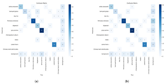
Figure 9.
(a) The confusion matrix of MKD8. (b) The confusion matrix of YOLOv8.
As shown in Table 11 and Table 12, MKD8 exhibits notable improvements over YOLOv8s in detecting specific weed categories. In particular, for Chenopodium album, MKD8 enhances mAP50 and mAP[50:95] by 33.8% and 33.5%, respectively. For reeds, the corresponding improvements are 35% and 26.6%, while for camel thorn, they are 6.1% and 5.1%. In the case of Chinese Ixeris denticulata, the improvements amount to 21.6% and 13.4%, respectively.
The issues of missed and false detections are further analyzed using the confusion matrix. In object-detection tasks, a confusion matrix is generated when the detection results meet the IoU threshold. The diagonal elements represent the number of correctly classified instances, while the lower left and upper right regions correspond to missed and false detections, respectively.
As depicted in Figure 9, MKD8 successfully detects 318 instances, whereas YOLOv8 detects 314 instances. This indicates that MKD8 achieves a slight reduction in missed and false detections compared to YOLOv8 on the given dataset.
4.8. Overfitting Analysis
It is evident from Table 3 and Table 6 that MKD8 demonstrates substantial improvements on the CornCottonWeed dataset. To assess whether the model exhibits signs of overfitting, we visualized the bounding box regression loss, distribution focal loss, and class loss during training on the CornCottonWeed dataset, as depicted in Figure 10.
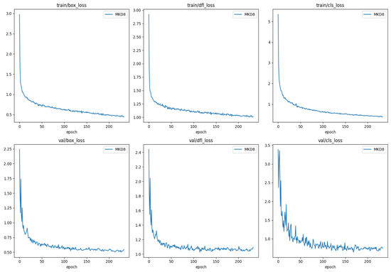
Figure 10.
MKD8 training process loss visualization on CornCottonWeed dataset. box_loss represents bounding box regression loss, dfl_loss represents distribution focal loss, and cls_loss represents class loss.
Specifically, both the bounding box regression loss and distribution focal loss are designed to optimize the predicted bounding box positions. The bounding box regression loss primarily focuses on enhancing the localization accuracy by refining the center point and IoU, while the distribution focal loss emphasizes fine-grained position optimization to capture local details. Meanwhile, the class loss quantifies the discrepancy between the predicted object class and the actual label, aiming to improve classification accuracy.
As illustrated in the upper three graphs of Figure 10, all three loss functions exhibit a gradual reduction and stable convergence throughout the training process, with negligible oscillations or upward trends, particularly toward the final training stages. This observation indicates that MKD8 has achieved a satisfactory fit on the training set. Although the CornCottonWeed dataset was divided into training, validation, and test sets at a ratio of 6:2:2 to retain sufficient samples in the validation and test sets, the inherent class imbalance still led to minor fluctuations in class loss during testing. However, the overall trend of class loss remains downward and gradually stabilizes, reflecting adequate model fitting on the validation set as well. Finally, combining all the images, the gap between the training loss and validation loss curves is always small, and there is no obvious separation, which means that the model does not “remember” the training data, but learns useful features and does not fall into overfitting.
5. Conclusions
In response to the current challenges in weed detection, such as the insufficiency of datasets and the high similarity between weeds and crops that makes model detection difficult, we initially collected weed images from cotton and corn fields to construct the CornCottonWeed dataset. Subsequently, we designed the MKD8 model for weed-detection tasks. The MKD8 model introduces the VSS module and KAN convolution, effectively addressing the issues of deep-feature loss and the challenge of capturing fine-grained semantic features by integrating global features with an adaptive activation function. Additionally, to mitigate the interference of background noise on model detection, we designed the ASDW module. By combining dynamic convolution with an attention mechanism, this module significantly enhances the model’s robustness against background noise. The experimental results indicate that the MKD8 model not only outperforms its peers but also maintains a leading position in comparison with other models. Overall, the CornCottonWeed dataset provides strong data support for the field of weed detection, and the development of the MKD8 model offers a new solution for weed-detection tasks in precision agriculture, marking significant progress in the field of weed detection.
Despite the CornCottonWeed dataset having certain limitations in terms of data volume and class balance, these challenges provide a clear direction for our future research. Specifically, we plan to delve into how data augmentation and algorithm optimization can effectively address the issues of insufficient data and class imbalance, thereby enhancing the model’s generalization capability and robustness.
Additionally, we will focus on the lightweight aspect of the MKD8 model. As deep-learning models are widely applied across various domains, the computational complexity and storage costs increasingly become key factors that constrain their practical deployment. Therefore, we intend to pursue model compression and knowledge distillation techniques to transform the MKD8 model into a more lightweight version, reducing its computational complexity and storage requirements while striving to maintain its performance to meet the demands of real-world applications.
Author Contributions
Conceptualization, W.S.; methodology, W.S.; validation, W.S.; writing—original draft preparation, W.S.; writing—review and editing, W.S., W.Y. and D.R.; resources, J.W.; supervision, J.W., D.C., D.R.; funding acquisition, W.Y. All authors have read and agreed to the published version of the manuscript.
Funding
This work was a research achievement supported by the National Key R&D Program of China Major Project (Grant No.2022ZD0115800). The Science and Technology Program of Xinjiang (Grant No.2022B01008). The National Science Foundation of China (Grant No.62341206).
Institutional Review Board Statement
Not applicable.
Data Availability Statement
The experimental data of this article can be obtained from the corresponding author. The CornCottonWeed image data involved in this paper was provided by Wang Jiajia’s team in our laboratory, and the data cleaning and labeling of the CornCottonWeed dataset were completed by the author. If you have any questions, please contact us at wjjxj@xju.edu.cn or 107552304135@xju.edu.cn.
Conflicts of Interest
The authors declare no conflicts of interest.
Appendix A. Visualization
Heatmaps serve as an effective tool for visualizing the activations of specific layers within neural networks, where the intensity of colors indicates the model’s degree of attention to particular features. By leveraging heatmaps, we can discern the model’s sensitivity to distinct features and examine the rationale behind the model’s predictions. In this study, we adopted four visualization techniques—XGradCAM [46,47], EigenCAM [46,48], HiResCAM [46,49], and RandomCAM [46]—to generate heatmaps for all models used in our experiments, as depicted in Figure A1. Furthermore, to gain deeper insights into the specific performance of MKD8 and YOLOv8, we conducted comprehensive visualizations of these two models, as illustrated in Figure A2.
By presenting heatmaps from four different methods, we found that the MKD8 model pays more attention to weed targets on both the CornCottonWeed and CottoWeed12 datasets. For a randomly selected image from the CottoWeed12 dataset, YOLOv8’s detection confidence was 0.96, while the MKD8 model achieved a target confidence of 0.97, which is a 1% increase in confidence. For a randomly selected image from the CornCottonWeed dataset, YOLOv8’s detection confidence was 0.95, and the MKD8 model achieved a target confidence of 0.97, which is a 2% increase in confidence.
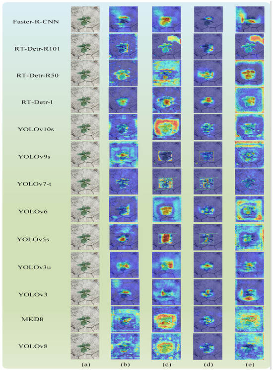
Figure A1.
The heatmaps from all models were derived using the following methods. (a) Input, (b) XGradCAM, (c) EigenCAM, (d) HiResCAM, and (e) RandomCAM. For heatmap, The darker the yellow on heatmap, the better the attention effect.
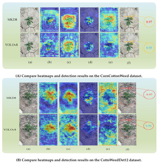
Figure A2.
Heatmaps and Detection Results. (a). Input, (b). XGradCAM, (c). EigenCAM, (d). HiResCAM, (e). RandomCAM and (f). Detection Result. For heatmap, The darker the yellow on heatmap, the better the attention effect.
Appendix B. Effective Receptive Field
Effective receptive field (ERF) [50] is indeed a critical concept in the realm of convolutional neural networks (CNNs), as it delineates the extent of the input image that influences a particular unit within the network. For object-detection models, the design of the ERF is especially significant because these models must be able to accurately identify and locate multiple objects within an image. This requirement necessitates that the model possesses an ERF large enough to encompass the target objects. Building upon the work of Ding and others, we conducted experiments to evaluate the ERF of our models. We compared the ERF of the YOLOv8 and MKD8 models. After randomly selecting 100 images from the CottoWeed12 dataset for our experiments, we obtained results for the ratio of the high contribution area within the minimum rectangle of contribution scores at thresholds (t) of 0.5 and 0.99. These results are presented in Table A1, which illustrates the performance of both models in capturing the essential features for object detection at different sensitivity levels.
Table A1.
High contribution area ratio of the minimum rectangles with different thresholds. Black bold font is the best effect.
Table A1.
High contribution area ratio of the minimum rectangles with different thresholds. Black bold font is the best effect.
| t = 50% | t = 99% | |
|---|---|---|
| r(YOLOv8s) | 24.5% | 97.2% |
| r(MKD8) | 24.8% | 98.4% |
Based on the data from Table A1, we can observe that the MKD8 model showed a 0.3% improvement in the ratio of the high contribution area within the minimum rectangle of contribution scores at a threshold (t) of 50% compared to the baseline model; at a threshold (t) of 99%, the improvement was 1.2%. Overall, the MKD8 model’s effective receptive field (ERF) demonstrated a noticeable enhancement over the YOLOv8 model’s ERF.
This improvement in ERF is significant as it indicates that the MKD8 model is more effective at capturing relevant features within the input image that contribute to accurate object detection. The increased ratio of high contribution areas at both thresholds suggests that the model is not only more sensitive to important features but also more robust in identifying objects across a wide range of feature intensities. This enhancement in the ERF is a testament to the effectiveness of the CVM, CKN, and ASDW modules in improving the model’s feature extraction and representation capabilities, leading to better detection performance.
Appendix C. Dataset Partitioning Results
Table A2.
The number of instances after dataset segmentation for the CornCottonWeed dataset.
Table A2.
The number of instances after dataset segmentation for the CornCottonWeed dataset.
| Category | Train | Val | Test |
|---|---|---|---|
| total | 1172 | 388 | 393 |
| White_Amaranth | 132 | 42 | 39 |
| Barnyard_Grass | 69 | 32 | 27 |
| Day_Lily | 28 | 10 | 16 |
| Portulaca_Oleracea | 245 | 96 | 83 |
| Dogwood | 145 | 43 | 45 |
| Gray_Quinoa | 277 | 83 | 99 |
| Chenopodium_Album | 24 | 7 | 2 |
| Reeds | 29 | 8 | 8 |
| Camel_Thorn | 204 | 65 | 64 |
| Chinese_Ixeris_Denticulata | 19 | 2 | 10 |
Table A3.
The number of instances after dataset segmentation for the CottoWeed12 dataset.
Table A3.
The number of instances after dataset segmentation for the CottoWeed12 dataset.
| Category | Train | Val | Test |
|---|---|---|---|
| total | 6087 | 1907 | 1394 |
| amaranthus_tuberculatus | 1248 | 426 | 285 |
| ipomoea_indica | 872 | 283 | 189 |
| euphorbia_maculata | 658 | 189 | 145 |
| portulaca_oleracea | 639 | 180 | 137 |
| eclipta | 604 | 212 | 146 |
| mollugo_verticillata | 576 | 172 | 148 |
| ambrosia_artemisiifolia | 600 | 154 | 111 |
| sida_rhombifolia | 305 | 101 | 80 |
| amaranthus_palmeri | 212 | 79 | 57 |
| senna_obtusifolia | 159 | 50 | 34 |
| eleusine_indica | 131 | 40 | 43 |
| physalis_angulata | 83 | 21 | 19 |
References
- Wang, A.; Zhang, W.; Wei, X. A review on weed detection using ground-based machine vision and image processing techniques. Comput. Electron. Agric. 2019, 158, 226–240. [Google Scholar]
- Zhang, H.; Wang, Z.; Guo, Y.; Ma, Y.; Cao, W.; Chen, D.; Yang, S.; Gao, R. Weed detection in peanut fields based on machine vision. Agriculture 2022, 12, 1541. [Google Scholar] [CrossRef]
- Zhang, W.; Miao, Z.; Li, N.; He, C.; Sun, T. Review of current robotic approaches for precision weed management. Curr. Robot. Rep. 2022, 3, 139–151. [Google Scholar] [PubMed]
- de Carvalho, S.J.P.; Nicolai, M.; Ferreira, R.R.; Figueira, A.V.d.O.; Christoffoleti, P.J. Herbicide selectivity by differential metabolism: Considerations for reducing crop damages. Sci. Agric. 2009, 66, 136–142. [Google Scholar]
- Pierce, F.J.; Nowak, P. Aspects of precision agriculture. Adv. Agron. 1999, 67, 1–85. [Google Scholar]
- Le, V.N.T.; Apopei, B.; Alameh, K. Effective plant discrimination based on the combination of local binary pattern operators and multiclass support vector machine methods. Inf. Process. Agric. 2019, 6, 116–131. [Google Scholar]
- Zhu, W.; Zhu, X. The application of support vector machine in veed classification. In Proceedings of the 2009 IEEE International Conference on Intelligent Computing and Intelligent Systems, Shanghai, China, 20–22 November 2009; IEEE: Piscataway, NJ, USA, 2009; Volume 4, pp. 532–536. [Google Scholar]
- Tang, J.L.; Chen, X.Q.; Miao, R.H.; Wang, D. Weed detection using image processing under different illumination for site-specific areas spraying. Comput. Electron. Agric. 2016, 122, 103–111. [Google Scholar]
- Midtiby, H.S.; Åstrand, B.; Jørgensen, O.; Jørgensen, R.N. Upper limit for context–based crop classification in robotic weeding applications. Biosyst. Eng. 2016, 146, 183–192. [Google Scholar]
- Zhang, X.; Xie, Z.; Zhang, N.; Cao, C. Weed recognition from pea seedling images and variable spraying control system. Nongye Jixie Xuebao (Trans. Chin. Soc. Agric. Mach.) 2012, 43, 220–225. [Google Scholar]
- Chen, Y.; Zhao, B.; Li, S.; Liu, L.; Yuan, Y.; Zhang, Y. Weed reverse positioning method and experiment based on multi-feature. Trans. Chin. Soc. Agric. Mach 2015, 46, 257–262. [Google Scholar]
- Wang, C.; Li, Z. Weed recognition using SVM model with fusion height and monocular image features. Trans. Chin. Soc. Agric. Eng. 2016, 32, 165–174. [Google Scholar]
- He, D.; Liang, Q.Y.; Pan, P.; Gao, G.; Li, H.; Tang, J. Weed recognition based on SVM-DS multi-feature fusion. Trans. Chin. Soc. Agric. Mach. 2013, 44, 182–187. [Google Scholar]
- Sabzi, S.; Abbaspour-Gilandeh, Y.; Arribas, J.I. An automatic visible-range video weed detection, segmentation and classification prototype in potato field. Heliyon 2020, 6, e03685. [Google Scholar]
- Deng, X.; Qi, L.; Ma, X.; Jiang, Y.; Chen, X.; Liu, H.; Chen, W. Recognition of weeds at seedling stage in paddy fields using multi-feature fusion and deep belief networks. Trans. Chin. Soc. Agric. Eng. 2018, 34, 165–172. [Google Scholar]
- Yu, J.; Sharpe, S.M.; Schumann, A.W.; Boyd, N.S. Deep learning for image-based weed detection in turfgrass. Eur. J. Agron. 2019, 104, 78–84. [Google Scholar]
- Potena, C.; Nardi, D.; Pretto, A. Fast and accurate crop and weed identification with summarized train sets for precision agriculture. In Proceedings of the Intelligent Autonomous Systems 14: Proceedings of the 14th International Conference IAS-14 14; Springer: Cham, Switzerland, 2017; pp. 105–121. [Google Scholar]
- Dyrmann, M.; Karstoft, H.; Midtiby, H.S. Plant species classification using deep convolutional neural network. Biosyst. Eng. 2016, 151, 72–80. [Google Scholar]
- Olsen, A.; Konovalov, D.A.; Philippa, B.; Ridd, P.; Wood, J.C.; Johns, J.; Banks, W.; Girgenti, B.; Kenny, O.; Whinney, J.; et al. DeepWeeds: A multiclass weed species image dataset for deep learning. Sci. Rep. 2019, 9, 2058. [Google Scholar]
- Chen, J.; Wang, H.; Zhang, H.; Luo, T.; Wei, D.; Long, T.; Wang, Z. Weed detection in sesame fields using a YOLO model with an enhanced attention mechanism and feature fusion. Comput. Electron. Agric. 2022, 202, 107412. [Google Scholar]
- Wu, H.; Wang, Y.; Zhao, P.; Qian, M. Small-target weed-detection model based on YOLO-V4 with improved backbone and neck structures. Precis. Agric. 2023, 24, 2149–2170. [Google Scholar]
- Fan, X.; Chai, X.; Zhou, J.; Sun, T. Deep learning based weed detection and target spraying robot system at seedling stage of cotton field. Comput. Electron. Agric. 2023, 214, 108317. [Google Scholar]
- Ahmad, A.; Saraswat, D.; Aggarwal, V.; Etienne, A.; Hancock, B. Performance of deep learning models for classifying and detecting common weeds in corn and soybean production systems. Comput. Electron. Agric. 2021, 184, 106081. [Google Scholar] [CrossRef]
- Fan, X.; Sun, T.; Chai, X.; Zhou, J. YOLO-WDNet: A lightweight and accurate model for weeds detection in cotton field. Comput. Electron. Agric. 2024, 225, 109317. [Google Scholar] [CrossRef]
- Jocher, G.; Chaurasia, A.; Qiu, J. Ultralytics YOLOv8. 2023. Available online: https://docs.ultralytics.com/models/yolov8/#citations-and-acknowledgements:~:text=%40software%7Byolov8_ultralytics,AGPL%2D3.0%7D%0A%7D (accessed on 6 March 2025).
- Liu, Y.; Tian, Y.; Zhao, Y.; Yu, H.; Xie, L.; Wang, Y.; Ye, Q.; Liu, Y. VMamba: Visual State Space Model. arXiv 2024, arXiv:2401.10166. [Google Scholar]
- Liu, Z.; Wang, Y.; Vaidya, S.; Ruehle, F.; Halverson, J.; Soljačić, M.; Hou, T.Y.; Tegmark, M. Kan: Kolmogorov-arnold networks. arXiv 2024, arXiv:2404.19756. [Google Scholar]
- Drokin, I. Kolmogorov-Arnold Convolutions: Design Principles and Empirical Studies. arXiv 2024, arXiv:2407.01092. [Google Scholar]
- Tawan. GRAM: KAN Meets Gram Polynomials. Website,2024. Available online: https://github.com/Khochawongwat/GRAMKAN?tab=readme-ov-file#gram-kan-meets-gram-polynomials (accessed on 6 March 2025).
- Dai, X.; Chen, Y.; Xiao, B.; Chen, D.; Liu, M.; Yuan, L.; Zhang, L. Dynamic Head: Unifying Object Detection Heads With Attentions. In Proceedings of the IEEE/CVF Conference on Computer Vision and Pattern Recognition (CVPR), Nashville, TN, USA, 19–25 June 2021; pp. 7373–7382. [Google Scholar]
- Wang, W.; Dai, J.; Chen, Z.; Huang, Z.; Li, Z.; Zhu, X.; Hu, X.; Lu, T.; Lu, L.; Li, H.; et al. Internimage: Exploring large-scale vision foundation models with deformable convolutions. In Proceedings of the IEEE/CVF Conference on Computer Vision and Pattern Recognition, Vancouver, BC, Canada, 17–24 June 2023; pp. 14408–14419. [Google Scholar]
- Chen, Y.; Dai, X.; Liu, M.; Chen, D.; Yuan, L.; Liu, Z. Dynamic relu. In Proceedings of the European Conference on Computer Vision, Glasgow, UK, 23–28 August 2020; Springer: Berlin/Heidelberg, Germany, 2020; pp. 351–367. [Google Scholar]
- Dang, F.; Chen, D.; Lu, Y.; Li, Z. YOLOWeeds: A novel benchmark of YOLO object detectors for multi-class weed detection in cotton production systems. Comput. Electron. Agric. 2023, 205, 107655. [Google Scholar] [CrossRef]
- Redmon, J. Yolov3: An incremental improvement. arXiv 2018, arXiv:1804.02767. [Google Scholar]
- Jocher, G.; Chaurasia, A.; Stoken, A.; Borovec, J.; Kwon, Y.; Michael, K.; Fang, J.; Yifu, Z.; Wong, C.; Montes, D.; et al. ultralytics/yolov5: v7. 0-yolov5 sota realtime instance segmentation. Zenodo. 2022. Available online: https://zenodo.org/records/7347926 (accessed on 6 March 2025).
- Li, C.; Li, L.; Jiang, H.; Weng, K.; Geng, Y.; Li, L.; Ke, Z.; Li, Q.; Cheng, M.; Nie, W.; et al. YOLOv6: A single-stage object detection framework for industrial applications. arXiv 2022, arXiv:2209.02976. [Google Scholar]
- Wang, C.Y.; Bochkovskiy, A.; Liao, H.Y.M. YOLOv7: Trainable bag-of-freebies sets new state-of-the-art for real-time object detectors. In Proceedings of the IEEE/CVF Conference on Computer Vision and Pattern Recognition, Vancouver, BC, Canada, 17–24 June 2023; pp. 7464–7475. [Google Scholar]
- Wang, C.Y.; Liao, H.Y.M. YOLOv9: Learning What You Want to Learn Using Programmable Gradient Information. In European Conference on Computer Vision; Springer: Berlin/Heidelberg, Germany, 2024. [Google Scholar]
- Wang, A.; Chen, H.; Liu, L.; Chen, K.; Lin, Z.; Han, J. YOLOv10: Real-Time End-to-End Object Detection. arXiv 2024, arXiv:2405.14458. [Google Scholar]
- Lv, W.; Xu, S.; Zhao, Y.; Wang, G.; Wei, J.; Cui, C.; Du, Y.; Dang, Q.; Liu, Y. DETRs Beat YOLOs on Real-time Object Detection. arXiv 2023, arXiv:2304.08069. [Google Scholar]
- Ren, S.; He, K.; Girshick, R.; Sun, J. Faster R-CNN: Towards real-time object detection with region proposal networks. IEEE Trans. Pattern Anal. Mach. Intell. 2016, 39, 1137–1149. [Google Scholar] [CrossRef] [PubMed]
- Xiong, Y.; Li, Z.; Chen, Y.; Wang, F.; Zhu, X.; Luo, J.; Wang, W.; Lu, T.; Li, H.; Qiao, Y.; et al. Efficient deformable convnets: Rethinking dynamic and sparse operator for vision applications. In Proceedings of the IEEE/CVF Conference on Computer Vision and Pattern Recognition, Seattle, WA, USA, 17–18 June 2024; pp. 5652–5661. [Google Scholar]
- Zhou, Q.; Wang, Z.; Zhong, Y.; Zhong, F.; Wang, L. Efficient Optimized YOLOv8 Model with Extended Vision. Sensors 2024, 24, 6506. [Google Scholar] [CrossRef] [PubMed]
- Zhou, Q.; Li, H.; Cai, Z.; Zhong, Y.; Zhong, F.; Lin, X.; Wang, L. YOLO-ACE: Enhancing YOLO with Augmented Contextual Efficiency for Precision Cotton Weed Detection. Sensors 2025, 25, 1635. [Google Scholar] [CrossRef]
- Guo, A.; Jia, Z.; Wang, J.; Zhou, G.; Ge, B.; Chen, W. A lightweight weed detection model with global contextual joint features. Eng. Appl. Artif. Intell. 2024, 136, 108903. [Google Scholar] [CrossRef]
- Gildenblat, J.; Contributors. PyTorch Library for CAM Methods. 2021. Available online: https://github.com/jacobgil/pytorch-grad-cam (accessed on 6 March 2025).
- Fu, R.; Hu, Q.; Dong, X.; Guo, Y.; Gao, Y.; Li, B. Axiom-Based Grad-CAM: Towards Accurate Visualization and Explanation of CNNs. arXiv 2020, arXiv:2008.02312. [Google Scholar]
- Muhammad, M.B.; Yeasin, M. Eigen-CAM: Class Activation Map using Principal Components. In Proceedings of the 2020 International Joint Conference on Neural Networks (IJCNN), Glasgow, UK, 19–24 July 2020; IEEE: Piscataway, NJ, USA, 2020. [Google Scholar] [CrossRef]
- Draelos, R.L.; Carin, L. Use HiResCAM Instead of Grad-CAM for Faithful Explanations of Convolutional Neural Networks. arXiv 2021, arXiv:2011.08891. [Google Scholar]
- Ding, X.; Zhang, X.; Han, J.; Ding, G. Scaling up your kernels to 31x31: Revisiting large kernel design in cnns. In Proceedings of the IEEE/CVF Conference on Computer Vision and Pattern Recognition, New Orleans, LA, USA, 18–24 June 2022; pp. 11963–11975. [Google Scholar]
Disclaimer/Publisher’s Note: The statements, opinions and data contained in all publications are solely those of the individual author(s) and contributor(s) and not of MDPI and/or the editor(s). MDPI and/or the editor(s) disclaim responsibility for any injury to people or property resulting from any ideas, methods, instructions or products referred to in the content. |
© 2025 by the authors. Licensee MDPI, Basel, Switzerland. This article is an open access article distributed under the terms and conditions of the Creative Commons Attribution (CC BY) license (https://creativecommons.org/licenses/by/4.0/).