A Network Bounded Adjusted Measure for Assessing the Efficiency of Agricultural and Pastoral Systems with Shared Factors and Undesirable Outputs

Abstract

The acts of assessing the efficiency of agricultural and pastoral systems and improving their production levels have profound implications for the sustainable development of the agricultural economy. Agricultural and pastoral systems are composed of agricultural sub-systems and pastoral sub-systems, which encompass both the production stage and the sales stage. These two sub-systems include shared factors and undesirable outputs, the latter of which refer to by-products such as CO₂ emissions, among others. These factors create significant challenges in assessing the efficiency of agricultural and pastoral systems. To address this issue, this study first proposes divisional system network bounded adjusted measure (BAM) models that consider shared factors and undesirable outputs for assessing the efficiency of agricultural sub-systems and pastoral sub-systems. Subsequently, an overall efficiency model for evaluating the efficiency of agricultural and pastoral systems is developed. The new method is applied to evaluate the efficiency of agricultural and pastoral systems across 30 provinces and cities in China. To explore the impact of undesirable outputs, the efficiency that ignores undesirable outputs is compared with our method. The results indicate that efficiency may be misestimated when ignoring undesirable outputs. Additionally, efficiency under different conditions of intermediate products is also computed, revealing that efficiency under the fixed link of intermediate products tends to be overestimated compared to the free link method we used.

1. Introduction

Agricultural and pastoral systems significantly impact the sustainable development of the agricultural economy. Specifically, these systems are composed of agricultural sub-systems and pastoral sub-systems, with the former primarily focusing on crop production and management and the latter focusing on livestock production and management. Furthermore, the two sub-systems encompass both the production stage and the sales stage. The production stage is responsible for creating the goods that people require, such as meat, eggs, and milk, while the sales stage is tasked with delivering the products generated by the production stage to consumers. Accurately assessing the efficiency of agricultural and pastoral systems, identifying weaknesses, and optimizing efficiency are profoundly significant for the long-term agricultural development of a nation. Therefore, evaluating the efficiency of agricultural and pastoral systems has become a focal point. For example, Martinsson et al. [1] measured the environmental effects of adopting automatic milking systems at the farm level. Sidhoum et al. [2] studied the impact of agri-environment measures on environmental and economic efficiency. Chen et al. [3] evaluated the production efficiency of agriculture across 30 provinces in China. Manogna and Aswini [4] explored the efficiency of grain agriculture productivity in 20 states of India.

Shared factors and undesirable outputs are two distinct factors widely present in agricultural and pastoral systems. Shared factors refer to resources that are not exclusively owned by a single sub-system but are consumed by several sub-systems. Although the total resources consumed are known, there is a lack of information regarding the exact amount consumed by each sub-system [5]. Commonly shared factors include labor, capital, and information. Undesirable outputs are the negative or unwanted outputs generated by decision-making units (DMUs) during the production process. These outputs are typically associated with adverse effects, such as environmental pollution and resource waste. In fact, undesirable outputs often exist as by-products of production, such as CO₂ and wastewater. The presence of these two kinds of factors adds complexity to measuring the efficiency of agricultural and pastoral systems. How to accurately evaluate the efficiency of agricultural and pastoral systems when shared factors and undesirable outputs coexist is currently a major challenge.

Data envelopment analysis (DEA) technology, proposed by Charnes et al. [6], is a nonparametric mathematical tool for evaluating the efficiency of DMUs. It is widely applied in fields such as logistics, ecosystems, urban development, and others. Nowadays, it is an effective tool for measuring the efficiency of agricultural and pastoral systems. After the first DEA model (known as the Charnes, Cooper, Rhodes (CCR) model [6]) was introduced, the radial DEA method underwent significant development. Non-radial DEA models also gained widespread application. Range adjusted measure (RAM), a weighted additive model, is a typical non-radial DEA model [7]. It addresses the boundary issues that may arise in traditional DEA models [8]. Based on the RAM model, Cooper et al. [9] developed the bounded adjusted measure (BAM), which is also a weighted additive model. The BAM model has a higher discriminatory power used to distinguish DMUs compared to the RAM model. It is applicable not only under the assumption of constant returns to scale (CRS) but also under the variable returns to scale (VRS) assumption. However, the current BAM method ignores shared factors and undesirable outputs. Given this, we propose novel BAM models that take into account both shared factors and undesirable outputs for measuring the efficiency of agricultural sub-systems, the efficiency of pastoral sub-systems, and the overall efficiency of agricultural and pastoral systems. Moreover, our new models consider both the production and sales stages of the agricultural and pastoral systems. This novel approach can assist decision-makers in identifying weak processes in agricultural and pastoral systems, enabling timely adjustments to production strategies and the optimization of system efficiency.

The organization of this paper is as follows: Section 2 discusses the literature from the perspective of shared factors, undesirable outputs, and BAM. Section 3 analyzes the production possibility sets (PPS) from the perspective of agricultural sub-systems, pastoral sub-systems, and agricultural and pastoral systems. Following this, the novel network BAM models used to evaluate divisional efficiency and overall efficiency are presented. Section 4 applies the proposed models to assess the efficiency of agricultural and pastoral systems across 30 provinces and cities in China. Section 5 calculates the efficiency when ignoring undesirable outputs (IUO). Efficiency under different conditions of intermediate products is also computed. Section 6 provides the conclusion of the paper.

2. Literature Review

2.1. Shared Factors

Currently, a majority of the literature on shared factors focuses on the application of radial models, such as Charnes, Cooper, Rhodes (CCR) and Banker, Charnes, Cooper (BCC), thereby neglecting non-radial models.

Table 1. The literature on shared factors.

Literature	Considering Shared Factors	Considering Undesirable Outputs	Models	Application Fields
Chen et al. [10]	Yes	No	BCC	Information technology
Zhang et al. [11]	Yes	No	CCR	Bank
Toloo et al. [12]	Yes	No	CCR	Bank
Zhu et al. [13]	Yes	No	CCR	Numerical example
Zhao et al. [14]	Yes	No	BCC	University
Wu et al. [15]	Yes	No	BCC	Industry
Wang et al. [16]	Yes	No	BCC	High-tech industry
Chen et al. [17]	Yes	No	BCC	High-tech industry
Lin and Lu [18]	Yes	No	BCC	Investment
An et al. [19]	Yes	No	BCC	Numerical example
Shabani and Shirazi [20]	Yes	No	BCC	Bank
Villa and Lozano [5]	Yes	No	SBI	Football
He and Zhu [21]	Yes	No	SBM	Industry
Chen et al. [22]	Yes	No	SBM	High-tech industry

summarizes the current literature on shared factors. It can be observed that Chen et al. [10], Zhang et al. [11], Toloo et al. [12], Zhu et al. [13]. Zhao et al. [14], Wu et al. [15], Wang et al. [16], Chen et al. [17], Lin and Lu [18], An et al. [19], and Shabani and Shirazi [20] all employed radial models to assess the efficiency of DMUs in the presence of shared factors, overlooking non-radial models. Furthermore, these studies also neglected the impact of undesirable outputs. It is important to emphasize that none of these studies has been applied to the agricultural sector, which is also a limitation.

Although some studies have proposed non-radial models to address shared factors, they have similarly overlooked the role of undesirable outputs. For instance, Villa and Lozano [5] developed a shared-inputs slacks-based inefficiency (SBI) model to evaluate the performance of football clubs, but they ignored undesirable outputs. He and Zhu [21] proposed a dynamic slacks-based measure (SBM) model considering shared inputs, but they also ignored undesirable outputs. Chen et al. [22] used a super-efficiency SBM model considering shared inputs for evaluating high-tech industry green innovation performance in China, where undesirable outputs were not included. Moreover, none of these studies has addressed agricultural and pastoral systems, which is another shortcoming that we intend to rectify.

In summary, the current literature on shared factors exhibits three main shortcomings: 1. the majority of studies exclusively utilize radial models, neglecting non-radial models; 2. the impact of undesirable outputs within the systems is overlooked; 3. the research has not been applied to agricultural and pastoral systems. To address these gaps, this paper proposes a non-radial model that takes into account shared factors and undesirable outputs for evaluating the efficiency of agricultural and pastoral systems.

2.2. Undesirable Outputs

In response to the specificity of undesirable outputs, the DEA field has proposed several methods to handle them. The first method is to consider undesirable outputs as inputs. Inputs are generally intended to be as small as possible to reduce costs. Similarly, undesirable outputs are also desired to be minimized. For this reason, many researchers treated undesirable outputs as inputs. Liu et al. [23] thought that it was beneficial to incorporate undesirable outputs as inputs. Izadikhah and Khoshroo [24] constructed a modified enhanced Russell model, in which undesirable outputs were treated as inputs. However, in practice, this method is often not accepted because it overlooks the characteristics of undesirable outputs. The second method is to deal with undesirable outputs under weak disposability (WD), which was presented by Fare et al. [25]. For example, Roshdi et al. [26] presented oriented distance functions for measuring environmental performance, and undesirable outputs were treated as weakly disposable. Li et al. [27] applied weak disposability when handling undesirable outputs to assess the performance of green suppliers. The third method is to cope with undesirable outputs based on the SBM. This method is widely used. For instance, Chen et al. [28] employed a RAM model with undesirable outputs to measure the performances of the truck restriction policy, and the undesirable outputs were coped with the SBM. Mirhedayatian et al. [29] presented a network SBM model in the presence of fuzzy data and undesirable outputs. Chen et al. [30] introduced a unified BAM considering undesirable outputs, which was handled by the SBM method.

The advantage of the SBM method is that it can provide additional information about the deviation of each undesirable output from the target under the condition that desirable outputs are maximized while undesirable outputs are minimized. Therefore, this method will be utilized in this study to cope with undesirable outputs, such as CO₂ emissions. Moreover, the aforementioned literature on undesirable outputs has overlooked the influence of shared factors. To address this gap, this paper incorporates shared undesirable outputs into the scope of research.

2.3. Bounded Adjusted Measure

BAM was developed by Cooper et al. [9]. It is an additive model and has been widely used across various fields. Now, the BAM model has undergone significant development. Rashidi and Saen [31] developed a BAM model that integrates undesirable outputs for assessing eco-efficiency. Pastor et al. [32] revised the boundaries of the BAM and presented an enhanced BAM for the CRS bounded additive model. Khoshroo et al. [33] developed a new approach based on the BAM model to evaluate the performance of tomato production and decrease the carbon footprint. Ma et al. [34] incorporated dual-role factors and undesirable factors into the network BAM model to assess the performance of automotive supply chains. Chen et al. [30] presented a unified BAM in the presence of undesirable outputs for measuring the corresponding production efficiency change of the highway transport sector. Wu et al. [35] used the BAM model to explore the impacts of fuel consumption and vehicle quantities in China’s highway transport.

However, the existing research on the BAM method has a limitation in that it does not simultaneously consider shared factors and undesirable outputs, which is one of the issues this study aims to address.

2.4. Efficiency of Agricultural and Pastoral Systems

Existing studies have employed diverse DEA approaches to assess the efficiency of agricultural and pastoral systems across varied contexts. Zhang et al. [36] applied the SBM model to assess agricultural carbon emission efficiency in the presence of undesirable outputs. Guo et al. [37] used the CCR method and the Malmquist index model to measure the efficiency of the agricultural circular economy. Manogna and Aswini [4] conducted an efficiency assessment of grain agricultural productivity in 20 states of India using the CCR model and the Malmquist productivity index. Nandy and Singh [38] estimated the efficiency of rice producers in eastern rural India using a fuzzy DEA method.

To the best of our knowledge, there is no literature that has applied BAM to agricultural and pastoral systems. Moreover, the existing studies did not simultaneously consider the impact of shared factors and undesirable outputs. To address these shortcomings, we propose a new BAM method that takes into account both shared factors and undesirable outputs.

3. Methods

3.1. Production Possibility Sets

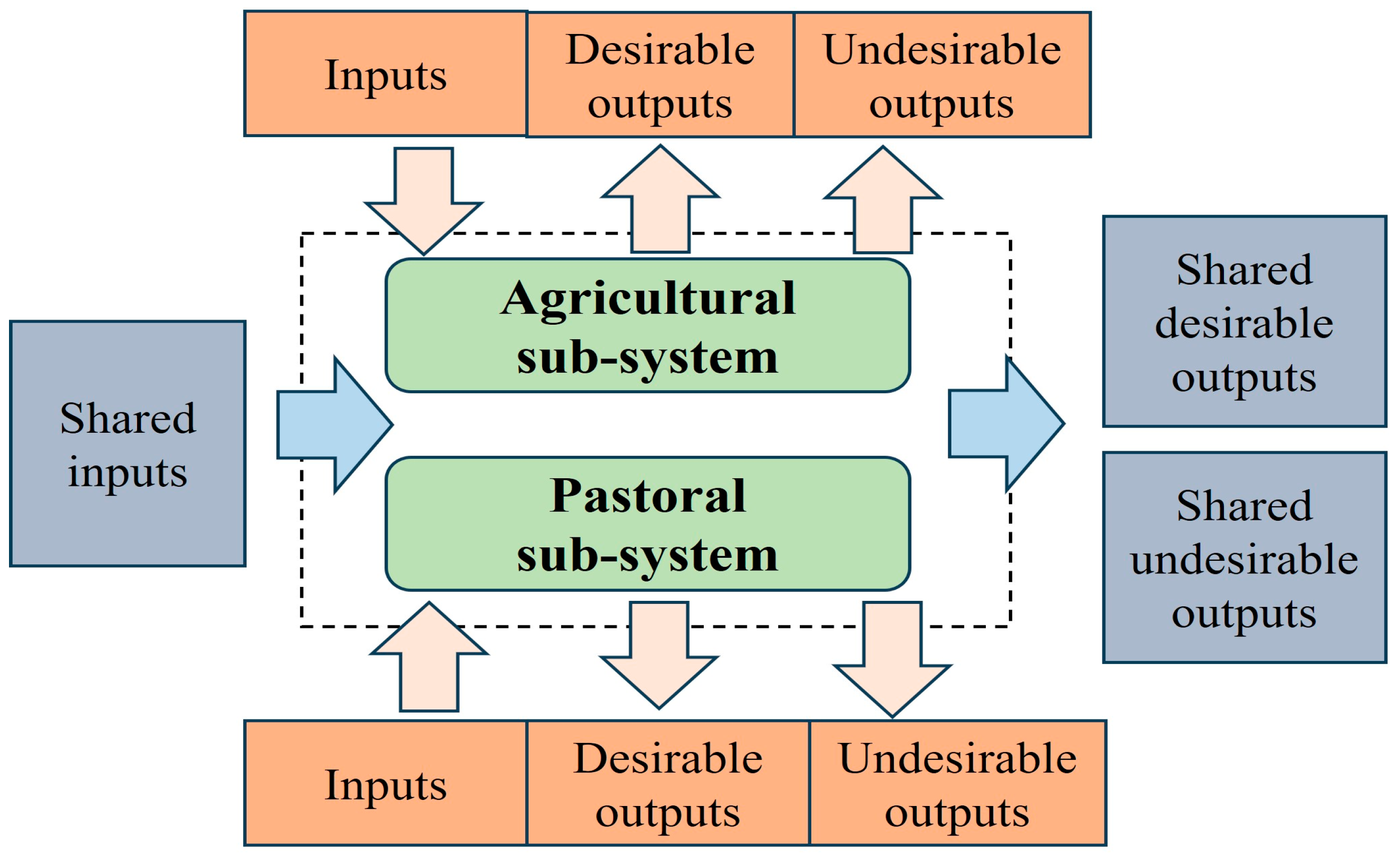
Agricultural and pastoral systems often exhibit an inseparable parallel structural process, which consists of an agricultural sub-system and a pastoral sub-system, as shown in Figure 1. Both the agricultural sub-system and the pastoral sub-system utilize inputs to generate desirable outputs and undesirable outputs. In addition to the factors exclusively owned by each sub-system, there are also factors jointly shared by the two sub-systems, known as shared factors. Both sub-systems typically have shared inputs, such as fixed asset investments, public infrastructure, number of employees, and diesel consumption. Regarding shared desirable outputs, there are total production value and overall profits. For shared undesirable outputs, there are also carbon dioxide emissions, wastewater discharge, areas of land degradation, and areas of soil contamination.

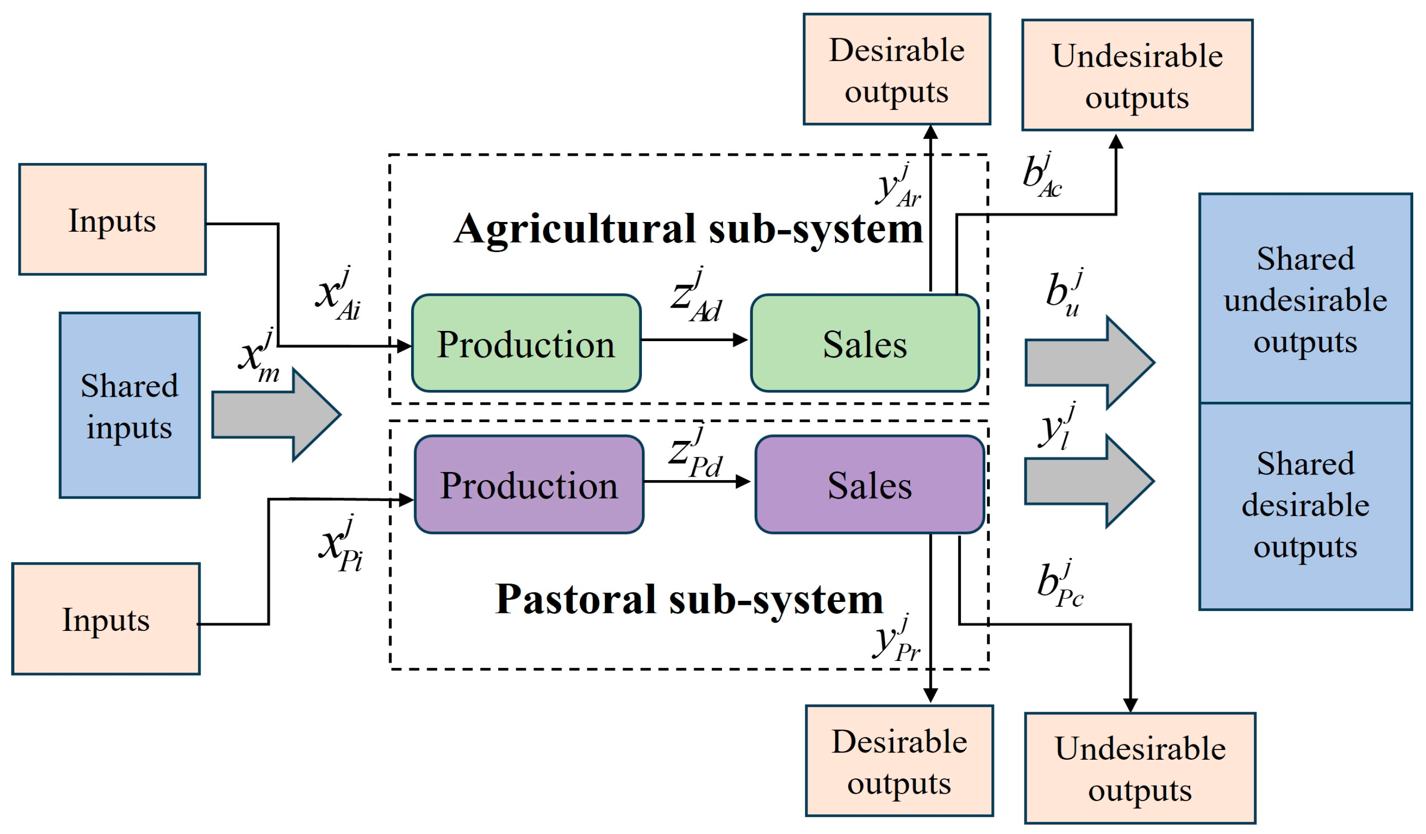
In Figure 1, the production process treats the agricultural and pastoral system as a black box. However, in reality, within the agricultural and pastoral system, these can be further divided into two sub-stages: production and sales. Figure 2 illustrates the production and sales stages within the agricultural and pastoral system. By observing Figure 2, it is evident that inputs for both the agricultural sub-system and the pastoral sub-system occur during the production stage, while desirable and undesirable outputs are realized during the sales stage. There are intermediate products between the production and sales stages.

Suppose that there are n agricultural and pastoral systems to be evaluated. ${DMU}^j(j=1,\dots ,n)$ indicates the jth agricultural and pastoral system, which includes an agricultural sub-system and a pastoral sub-system.

Table 2. Definitions of the variables in Figure 2.

Variables	Definition
$x_{ki}^j(i=1,\dots ,I_k)$	The ith input of the k sub-system
$y_{kr}^j(r=1,\dots ,S_k)$	The rth desirable output of the k sub-system
$z_{kd}^j(d=1,\dots ,D_k)$	The dth intermediate product from the production stage to the sales stage of the k sub-system
$b_{kc}^j(c=1,\dots ,C_k)$	The cth undesirable output of the k sub-system
$x_m^j(m=1,\dots ,M)$	The mth shared input of the agricultural sub-system and the pastoral sub-system
$y_l^j(l=1,\dots ,L)$	The lth shared desirable output of the agricultural sub-system and the pastoral sub-system
$b_u^j(u=1,\dots ,U)$	The uth shared undesirable output of the agricultural sub-system and the pastoral sub-system
$k=A$	The agricultural sub-system
$k=P$	The pastoral sub-system

summarizes the definitions of the variables in Figure 2.

Now, we analyze the PPS of the agricultural and pastoral system. For the agricultural sub-system, define the following vectors: $X_A=(x_{A1},\dots ,x_{A{I}_A})\in R_{+}^{I_A}$, $Y_A=(y_{A1},\dots ,y_{A{S}_A})\in R_{+}^{S_A}$, $B_A=(b_{A1},\dots ,b_{A{C}_A})\in R_{+}^{C_A}$, $Z_A=(z_{A1},\dots ,z_{A{d}_A})\in R_{+}^{D_A}$, For the pastoral sub-system, we define: $X_P=(x_{P1},\dots ,x_{P{I}_P})\in R_{+}^{I_P}$, $Y_P=(y_{P1},\dots ,y_{P{S}_P})\in R_{+}^{S_P}$, $B_P=(b_{P1},\dots ,b_{P{C}_P})\in R_{+}^{C_P}$, $Z_P=(z_{P1},\dots ,z_{P{d}_P})\in R_{+}^{D_P}$. For shared factors, define: $X=(x_1,\dots ,x_M)\in R_{+}^M$, $Y=(y_1,\dots ,y_L)\in R_{+}^{\mathrm{L}}$, $B=(b_1,\dots ,b_U)\in R_{+}^{\mathrm{U}}$.

For the agricultural sub-system, we can obtain PPS (1) $\left\{(X_A,Y_A,B_A,Z_A,X,Y,B)\right\}$:

$$\left\{\begin{array}{l}{\displaystyle {\sum }_{j=1}^n{\lambda }_{A1}^j{X}_A^j\le X_A},{\displaystyle {\sum }_{j=1}^n{\lambda }_{A2}^j{Y}_A^j\ge Y_A},{\displaystyle {\sum }_{j=1}^n{\lambda }_{A2}^j{B}_A^j\le B_A,}{\displaystyle {\sum }_{j=1}^n{\lambda }_{A1}^j{\alpha }_A{X}^j\le {\alpha }_{A}X,}{\displaystyle {\sum }_{j=1}^n{\lambda }_{A2}^j{\beta }_A{Y}^j\ge {\beta }_{A}Y},\\ {\displaystyle {\sum }_{j=1}^n{\lambda }_{A2}^j{\mu }_A{B}^j\le {\mu }_{A}B},{\displaystyle {\sum }_{j=1}^n{\lambda }_{A1}^j{Z}_A^j=Z_A,}{\displaystyle {\sum }_{j=1}^n{\lambda }_{A2}^j{Z}_A^j=Z_A,}{\displaystyle {\sum }_{j=1}^n{\lambda }_{A1}^j=1},{\displaystyle {\sum }_{j=1}^n{\lambda }_{A2}^j=1}\end{array}\right\}$$

(1)

where ${\lambda }_{A1}^j$ denotes the intensity in the production stage of the agricultural sub-system. ${\lambda }_{A2}^j$ denotes the intensity in the sales stage of the agricultural sub-system. ${\alpha }_A$ is the proportion of shared inputs allocated to the production stage of the agricultural sub-system. ${\beta }_A$ is the proportion of shared desirable outputs allocated to the sales stage of the agricultural sub-system. ${\mu }_A$ is the proportion of shared undesirable outputs allocated to the sales stage of the agricultural sub-system. Constraints ${\displaystyle {\sum }_{j=1}^n{\lambda }_{A1}^j=1}$ and ${\displaystyle {\sum }_{j=1}^n{\lambda }_{A2}^j=1}$ denote that the process of the agricultural sub-system is under the assumption of VRS.

For the pastoral sub-system, there exists the following PPS $\left\{(X_P,Y_P,B_P,Z_P,X,Y,B)\right\}$:

$$\left\{\begin{array}{l}{\displaystyle {\sum }_{j=1}^n{\lambda }_{P1}^j{X}_P^j\le X_P},{\displaystyle {\sum }_{j=1}^n{\lambda }_{P2}^j{Y}_P^j\ge Y_P},{\displaystyle {\sum }_{j=1}^n{\lambda }_{P2}^j{B}_P^j\le B_P,}{\displaystyle {\sum }_{j=1}^n{\lambda }_{P1}^j{\alpha }_P{X}^j\le {\alpha }_{P}X,}\\ {\displaystyle {\sum }_{j=1}^n{\lambda }_{P2}^j{\beta }_P{Y}^j\ge {\beta }_{P}Y},{\displaystyle {\sum }_{j=1}^n{\lambda }_{P2}^j{\mu }_P{B}^j\le {\mu }_{P}B,}{\displaystyle {\sum }_{j=1}^n{\lambda }_{P1}^j{Z}_P^j=Z_P,}{\displaystyle {\sum }_{j=1}^n{\lambda }_{P2}^j{Z}_P^j=Z_P,}\\ {\displaystyle {\sum }_{j=1}^n{\lambda }_{P1}^j=1},{\displaystyle {\sum }_{j=1}^n{\lambda }_{P2}^j=1}\end{array}\right\}$$

(2)

In PPS (2), ${\lambda }_{P1}^j$ denotes the intensity in the production stage of the pastoral sub-system. ${\lambda }_{P2}^j$ denotes the intensity in the sales stage of the pastoral sub-system. ${\alpha }_P$ is the proportion of shared inputs allocated to the production stage of the pastoral sub-system. ${\beta }_P$ is the proportion of shared desirable outputs allocated to the sales stage of the pastoral sub-system. ${\mu }_P$ is the proportion of shared undesirable outputs allocated to the sales stage of the pastoral sub-system. Constraints ${\displaystyle {\sum }_{j=1}^n{\lambda }_{P1}^j=1}$ and ${\displaystyle {\sum }_{j=1}^n{\lambda }_{P2}^j=1}$ denote that the process of the pastoral sub-system is under the assumption of VRS.

From an overall perspective, if we consider the agricultural sub-system and the pastoral sub-system as a whole, the following PPS (3) can be obtained.$\left\{(X_A,Y_A,B_A,X_P,Y_P,B_P,Z_A,Z_P,X,Y,B)\right\}$:

$$\left\{\begin{array}{l}{\displaystyle {\sum }_{j=1}^n{\lambda }_{A1}^j{X}_A^j\le X_A},{\displaystyle {\sum }_{j=1}^n{\lambda }_{A2}^j{Y}_A^j\ge Y_A},{\displaystyle {\sum }_{j=1}^n{\lambda }_{A2}^j{B}_A^j\le B_A,}{\displaystyle {\sum }_{j=1}^n{\lambda }_{A1}^j{\alpha }_A{X}^j\le {\alpha }_{A}X,}\\ {\displaystyle {\sum }_{j=1}^n{\lambda }_{A2}^j{\beta }_A{Y}^j\ge {\beta }_{A}Y},{\displaystyle {\sum }_{j=1}^n{\lambda }_{A2}^j{\mu }_A{B}^j\le {\mu }_{A}B,}{\displaystyle {\sum }_{j=1}^n{\lambda }_{A1}^j{Z}_A^j=Z_A,}{\displaystyle {\sum }_{j=1}^n{\lambda }_{A2}^j{Z}_A^j=Z_A,}\\ {\displaystyle {\sum }_{j=1}^n{\lambda }_{P1}^j{X}_P^j\le X_P},{\displaystyle {\sum }_{j=1}^n{\lambda }_{P2}^j{Y}_P^j\ge Y_P},{\displaystyle {\sum }_{j=1}^n{\lambda }_{P2}^j{B}_P^j\le B_P,}{\displaystyle {\sum }_{j=1}^n{\lambda }_{P1}^j{Z}_P^j=Z_P,}\\ {\displaystyle {\sum }_{j=1}^n{\lambda }_{P2}^j{Z}_P^j=Z_P,}{\displaystyle {\sum }_{j=1}^n{\lambda }_{P1}^j{\alpha }_P{X}^j\le {\alpha }_{P}X,}{\displaystyle {\sum }_{j=1}^n{\lambda }_{P2}^j{\beta }_P{Y}^j\ge {\beta }_{P}Y},\\ {\displaystyle {\sum }_{j=1}^n{\lambda }_{P2}^j{\mu }_P{B}^j\le {\mu }_{P}B,}{\displaystyle {\sum }_{j=1}^n{\lambda }_{A1}^j=1},{\displaystyle {\sum }_{j=1}^n{\lambda }_{A2}^j=1},{\displaystyle {\sum }_{j=1}^n{\lambda }_{P1}^j=1},{\displaystyle {\sum }_{j=1}^n{\lambda }_{P2}^j=1}\end{array}\right\}$$

(3)

It should be specified that, for PPS (3), there are the following equations: ${\alpha }_A+{\alpha }_P=1$, ${\beta }_A+{\beta }_P=1$, ${\mu }_A+{\mu }_P=1$.

3.2. Divisional Efficiency Models

Section 3.1 analyzes the PPS of agricultural sub-systems. Based on the BAM and PPS (1), we can present the BAM model considering shared factors and undesirable outputs for measuring the efficiency of the agricultural sub-system. The model can be expressed as follows (Model (4)).

Table 3. Definitions of the variables in Model (4).

Variables	Definition
$s_{Ai}^{-}$	The slack of inputs in the agricultural sub-system
$s_{Ar}^{+}$	The slack of desirable outputs in the agricultural sub-system
$s_{Ac}^{-}$	The slack of undesirable outputs in the agricultural sub-system
$s_{Am}^{-}$	The slack of shared inputs in the agricultural sub-system
$s_{Al}^{+}$	The slack of shared desirable outputs in the agricultural sub-system
$s_{Au}^{-}$	The slack of shared undesirable outputs in the agricultural sub-system
${\sigma }_{A1}$	Weight of the production stage
${\sigma }_{A2}$	Weight of the sales stage
${\alpha }_{Am}$	The proportion of the mth shared input allocated to the agricultural sub-system
${\beta }_{Al}$	The proportion of the lth shared desirable output allocated to the agricultural sub-system
${\mu }_{Au}$	The proportion of the uth shared undesirable output allocated to the agricultural sub-system
$B_{Ai}^{-}$	The lower-sided range for the ith input in the agricultural sub-system
$B_{Ar}^{+}$	The upper-sided range for the rth desirable output in the agricultural sub-system
$B_{Ac}^{-}$	The lower-sided range for the cth undesirable output in the agricultural sub-system
$B_{Am}^{-}$	The lower-sided range for the mth shared input in the agricultural sub-system
$B_{Al}^{+}$	The upper-sided range for the lth shared desirable output in the agricultural sub-system
$B_{Au}^{-}$	The lower-sided range for the uth shared undesirable output in the agricultural sub-system

summarizes the definitions of the variables in Model (4).

$$\begin{array}{l}{E}_A=\min 1-{\displaystyle \frac{{\sigma }_{A1}}{I_A+M}}({\displaystyle \sum _{i=1}^{I_A}\frac{s_{Ai}^{-}}{B_{Ai}^{-}}+}{\displaystyle \sum _{m=1}^M\frac{s_{Am}^{-}}{B_{Am}^{-}}})-{\displaystyle \frac{{\sigma }_{A2}}{S_A+C_A+L+U}}({\displaystyle \sum _{r=1}^{S_A}\frac{s_{Ar}^{+}}{B_{Ar}^{+}}}+{\displaystyle \sum _{c=1}^{C_A}\frac{s_{Ac}^{-}}{B_{Ac}^{-}}}+{\displaystyle \sum _{l=1}^L\frac{s_{Al}^{+}}{B_{Al}^{+}}}+{\displaystyle \sum _{u=1}^U\frac{s_{Au}^{-}}{B_{Au}^{-}}})\\ s.t.\\ {\displaystyle \sum _{j=1}^n{\lambda }_{A1}^j{x}_{Ai}^j}+s_{Ai}^{-}=x_{Ai}^o,i=1,2,\dots ,I_A\\ {\displaystyle \sum _{j=1}^n{\lambda }_{A2}^j{y}_{Ar}^j}-s_{Ar}^{+}=y_{Ar}^o,r=1,2,\dots ,S_A\\ {\displaystyle \sum _{j=1}^n{\lambda }_{A2}^j{b}_{Ac}^j}+s_{Ac}^{-}=b_{Ac}^o,c=1,2,\dots ,C_A\\ {\displaystyle \sum _{j=1}^n{\lambda }_{A1}^j{z}_{Ad}^j}={\displaystyle \sum _{j=1}^n{\lambda }_{A2}^j{z}_{Ad}^j},d=1,2,\dots ,D_A\\ {\displaystyle \sum _{j=1}^n{\lambda }_{A1}^j{\alpha }_{Am}{x}_m^j}+s_{Am}^{-}={\alpha }_{Am}{x}_m^o,m=1,2,\dots ,M\\ {\displaystyle \sum _{j=1}^n{\lambda }_{A2}^j{\beta }_{Al}{y}_l^j}-s_{Al}^{+}={\beta }_{Al}{y}_l^o,l=1,2,\dots ,L\\ {\displaystyle \sum _{j=1}^n{\lambda }_{A2}^j{\mu }_{Au}{b}_u^j}+s_{Au}^{-}={\mu }_{Au}{b}_u^o,u=1,2,\dots ,U\\ {\displaystyle \sum _{j=1}^n{\lambda }_{A1}^j=1},{\displaystyle \sum _{j=1}^n{\lambda }_{A2}^j=1},j=1,2,\dots ,n\\ s_{Ai}^{-},s_{Ar}^{+},s_{Ac}^{-},s_{Am}^{-},s_{Al}^{+},s_{Au}^{-},{\lambda }_{A1}^j,{\lambda }_{A2}^j\ge 0\end{array}$$

(4)

There exist: $B_{Ai}^{-}$ = $x_{Ai}^o$ − min ($x_{Ai}^j$), $B_{Ar}^{+}$ = max ($y_{Ar}^j$) − $y_{Ar}^o$, $B_{Ac}^{-}$ = $x_{Ac}^o$ − min ($x_{Ac}^j$), $B_{Am}^{-}$ = ${\alpha }_{Am}{x}_m^o$ − min (${\alpha }_{Am}{x}_m^j$), $B_{Al}^{+}$ = max (${\beta }_{Al}{y}_l^j$) − ${\beta }_{Al}{y}_l^o$, $B_{Al}^{-}$ = ${\mu }_{Au}{b}_u^o$ − min (${\mu }_{Au}{b}_u^j$). Constraint ${\displaystyle \sum _{j=1}^n{\lambda }_{A1}^j{z}_{Ad}^j}={\displaystyle \sum _{j=1}^n{\lambda }_{A2}^j{z}_{Ad}^j}$ represents the free link. The SBM method is applied to deal with undesirable outputs.

Assume that $s_{Ai}^{*-}$, $s_{Ar}^{*+}$, $s_{Ac}^{*-}$, $s_{Am}^{*-}$, $s_{Al}^{*+}$, and $s_{Au}^{*-}$ are the optimal values in Model (4). Equations (5) and (6) exist as follows:

$$E_{AP}=1-{\displaystyle \frac{1}{I_A+M}}({\displaystyle \sum _{i=1}^{I_A}\frac{s_{Ai}^{*-}}{B_{Ai}^{-}}+}{\displaystyle \sum _{m=1}^M\frac{s_{Am}^{*-}}{B_{Am}^{-}}})$$

(5)

$$E_{AS}=1-{\displaystyle \frac{1}{S_A+C_A+L+U}}({\displaystyle \sum _{r=1}^{S_A}\frac{s_{Ar}^{*+}}{B_{Ar}^{+}}}+{\displaystyle \sum _{c=1}^{C_A}\frac{s_{Ac}^{*-}}{B_{Ac}^{-}}}+{\displaystyle \sum _{l=1}^L\frac{s_{Al}^{*+}}{B_{Al}^{+}}}+{\displaystyle \sum _{u=1}^U\frac{s_{Au}^{*-}}{B_{Au}^{-}}})$$

(6)

where $E_{AP}$ is the production efficiency of the agricultural sub-system. $E_{AS}$ is the sales efficiency of the agricultural sub-system.

$E_A$ can also be expressed as the weighted arithmetic mean of the production efficiency and sales efficiency. It can be represented by the following Equation (7):

$$E_A={\sigma }_{A1}{E}_{AP}+{\sigma }_{A2}{E}_{AS}$$

(7)

Section 3.1 also analyzes the PPS of the pastoral sub-system. Based on the BAM and PPS (2), we can present the BAM model considering shared factors and undesirable outputs for the pastoral sub-system. The model can be expressed as follows (Model (8)).

Table 4. Definitions of the variables in Model (8).

Variables	Definition
$s_{Pi}^{-}$	The slack of inputs in the pastoral sub-system
$s_{Pr}^{+}$	The slack of desirable outputs in the pastoral sub-system
$s_{Pc}^{-}$	The slack of undesirable outputs in the pastoral sub-system
$s_{Pm}^{-}$	The slack of shared inputs in the pastoral sub-system
$s_{Pl}^{+}$	The slack of shared desirable outputs in the pastoral sub-system
$s_{Pu}^{-}$	The slack of shared undesirable outputs in the pastoral sub-system
${\sigma }_{P1}$	Weight of the production stage
${\sigma }_{P2}$	Weight of the sales stage
${\alpha }_{Pm}$	The proportion of the mth shared input allocated to the pastoral sub-system
${\beta }_{Pl}$	The proportion of the lth shared desirable output allocated to the pastoral sub-system
${\mu }_{Pu}$	The proportion of the uth shared undesirable output allocated to the pastoral sub-system
$B_{Pi}^{-}$	The lower-sided range for the ith input in the pastoral sub-system
$B_{Pr}^{+}$	The upper-sided range for the rth desirable output in the pastora sub-system
$B_{Pc}^{-}$	The lower-sided range for the cth undesirable output in the pastoral sub-system
$B_{Pm}^{-}$	The lower-sided range for the mth shared input in the pastoral sub-system
$B_{Pl}^{+}$	The upper-sided range for the lth shared desirable output in the pastoral sub-system
$B_{Pu}^{-}$	The lower-sided range for the uth shared undesirable output in the pastoral sub-system

summarizes the definitions of the variables in Model (8).

$$\begin{array}{l}{E}_P=\min 1-{\displaystyle \frac{{\sigma }_{P1}}{I_P+M}}({\displaystyle \sum _{i=1}^{I_P}\frac{s_{Pi}^{-}}{B_{Pi}^{-}}+}{\displaystyle \sum _{m=1}^M\frac{s_{Pm}^{-}}{B_{Pm}^{-}}})-{\displaystyle \frac{{\sigma }_{P2}}{S_P+C_P+L+U}}({\displaystyle \sum _{r=1}^{S_P}\frac{s_{Pr}^{+}}{B_{Pr}^{+}}}+{\displaystyle \sum _{c=1}^{C_P}\frac{s_{Pc}^{-}}{B_{Pc}^{-}}}+{\displaystyle \sum _{l=1}^L\frac{s_{Pl}^{+}}{B_{Pl}^{+}}}+{\displaystyle \sum _{u=1}^U\frac{s_{Pu}^{-}}{B_{Pu}^{-}}})\\ s.t.\\ {\displaystyle \sum _{j=1}^n{\lambda }_{P1}^j{x}_{Pi}^j}+s_{Pi}^{-}=x_{Pi}^o,i=1,2,\dots ,I_P\\ {\displaystyle \sum _{j=1}^n{\lambda }_{P2}^j{y}_{Pr}^j}-s_{Pr}^{+}=y_{Pr}^o,r=1,2,\dots ,S_P\\ {\displaystyle \sum _{j=1}^n{\lambda }_{P2}^j{b}_{Pc}^j}+s_{Pc}^{-}=b_{Pc}^o,c=1,2,\dots ,C_P\\ {\displaystyle \sum _{j=1}^n{\lambda }_{P1}^j{z}_{Pd}^j}={\displaystyle \sum _{j=1}^n{\lambda }_{P2}^j{z}_{Pd}^j},d=1,2,\dots ,D_P\\ {\displaystyle \sum _{j=1}^n{\lambda }_{P1}^j{\alpha }_{Pm}{x}_m^j}+s_{Pm}^{-}={\alpha }_{Pm}{x}_m^o,m=1,2,\dots ,M\\ {\displaystyle \sum _{j=1}^n{\lambda }_{P2}^j{\beta }_{Pl}{y}_l^j}-s_{Pl}^{+}={\beta }_{Pl}{y}_l^o,l=1,2,\dots ,L\\ {\displaystyle \sum _{j=1}^n{\lambda }_{P2}^j{\mu }_{Pu}{b}_u^j}+s_{Pu}^{-}={\mu }_{Pu}{b}_u^o,u=1,2,\dots ,U\\ {\displaystyle \sum _{j=1}^n{\lambda }_{P1}^j=1},{\displaystyle \sum _{j=1}^n{\lambda }_{P2}^j=1},j=1,2,\dots ,n\\ s_{P{i}_P}^{-},s_{P{r}_P}^{+},s_{P{c}_P}^{-},s_{Pm}^{-},s_{Pl}^{+},s_{Pu}^{-},{\lambda }_{P1}^j,{\lambda }_{P2}^j\ge 0\end{array}$$

(8)

The following exist: $B_{Pi}^{-}$ = $x_{Pi}^o$ − min ($x_{Pi}^j$), $B_{Pr}^{+}$ = max ($y_{Pr}^j$) − $y_{Pr}^o$, $B_{Pc}^{-}$ = $x_{Pc}^o$ − min ($x_{Pc}^j$), $B_{Pm}^{-}$ = ${\alpha }_{Pm}{x}_m^o$ − min (${\alpha }_{Pm}{x}_m^j$), $B_{Pl}^{+}$ = max (${\beta }_{Pl}{y}_l^j$) − ${\beta }_{Pl}{y}_l^o$, and $B_{Pu}^{-}$ = ${\mu }_{Pu}{b}_u^o$ − min (${\mu }_{Pu}{b}_u^j$).

Let $s_{Pi}^{*-}$, $s_{Pr}^{*+}$, $s_{Pc}^{*-}$, $s_{Pm}^{*-}$, $s_{Pl}^{*+}$, and $s_{Pu}^{*-}$ be the optimal values in Model (8). The following formulas (Equations (9) and (10)) exist:

$$E_{PP}=1-{\displaystyle \frac{1}{I_P+M}}({\displaystyle \sum _{i=1}^{I_P}\frac{s_{Pi}^{*-}}{B_{Pi}^{-}}+}{\displaystyle \sum _{m=1}^M\frac{s_{Pm}^{*-}}{B_{Pm}^{-}}})$$

(9)

$$E_{PS}=1-{\displaystyle \frac{1}{S_P+C_P+L+U}}({\displaystyle \sum _{r=1}^{S_P}\frac{s_{Pr}^{*+}}{B_{Pr}^{+}}}+{\displaystyle \sum _{c=1}^{C_A}\frac{s_{Pc}^{*-}}{B_{Pc}^{-}}}+{\displaystyle \sum _{l=1}^L\frac{s_{Pl}^{*+}}{B_{Pl}^{+}}}+{\displaystyle \sum _{u=1}^U\frac{s_{Pu}^{*-}}{B_{Pu}^{-}}})$$

(10)

$E_{PP}$ is the production efficiency of the pastoral sub-system. $E_{PS}$ is the sales efficiency of the pastoral sub-system.

Similar to Equation (7), $E_P$ can also be expressed as Equation (11) as follows:

$$E_P={\sigma }_{P1}{E}_{PP}+{\sigma }_{P2}{E}_{PS}$$

(11)

3.3. Overall Efficiency Model

Divisional efficiency models are proposed in Section 3.2. Now, we can develop the network BAM model considering shared factors and undesirable outputs to measure the overall efficiency based on PPS (3). It can be expressed as follows (Model (12)).

$$\begin{array}{l}E=\min 1-{\displaystyle \sum _k{w}_k}({\displaystyle \frac{{\sigma }_{k1}}{I_k+M}}({\displaystyle \sum _{i=1}^{I_k}\frac{s_{ki}^{-}}{B_{ki}^{-}}+}{\displaystyle \sum _{m=1}^M\frac{s_{km}^{-}}{B_{km}^{-}}})-{\displaystyle \frac{{\sigma }_{k2}}{S_k+C_k+L+U}}({\displaystyle \sum _{r_k=1}^{S_k}\frac{s_{kr}^{+}}{B_{kr}^{+}}}+{\displaystyle \sum _{c_k=1}^{C_k}\frac{s_{kc}^{-}}{B_{kc}^{-}}}+{\displaystyle \sum _{l=1}^L\frac{s_{ku}^{+}}{B_{kl}^{+}}}+{\displaystyle \sum _{u=1}^U\frac{s_{ku}^{-}}{B_{ku}^{-}}}))\\ s.t.\\ {\displaystyle \sum _{j=1}^n{\lambda }_{k1}^j{x}_{ki}^j}+s_{ki}^{-}=x_{ki}^o,i=1,2,\dots ,I_k\\ {\displaystyle \sum _{j=1}^n{\lambda }_{k2}^j{y}_{k{r}_k}^j}-s_{k{r}_k}^{+}=y_{k{r}_k}^o,r=1,2,\dots ,S_k\\ {\displaystyle \sum _{j=1}^n{\lambda }_{k2}^j{b}_{kc}^j}+s_{kc}^{-}=b_{kc}^o,c=1,2,\dots ,C_k\\ {\displaystyle \sum _{j=1}^n{\lambda }_{k1}^j{z}_{kd}^j}={\displaystyle \sum _{j=1}^n{\lambda }_{k2}^j{z}_{kd}^j},d=1,2,\dots ,D_k\\ {\displaystyle \sum _{j=1}^n{\lambda }_{k1}^j{\alpha }_{km}{x}_m^j}+s_{km}^{-}={\alpha }_{km}{x}_m^o,m=1,2,\dots ,M\\ {\displaystyle \sum _{j=1}^n{\lambda }_{k2}^j{\beta }_{kl}{y}_l^j}-s_{kl}^{+}={\beta }_{kl}{y}_l^o,l=1,2,\dots ,L\\ {\displaystyle \sum _{j=1}^n{\lambda }_{k2}^j{\mu }_{ku}{b}_u^j}+s_{ku}^{-}={\mu }_{ku}{b}_u^o,u=1,2,\dots ,U\\ {\displaystyle \sum _k{\alpha }_{km}=1,}{\displaystyle \sum _k{\beta }_{kl}=1,}{\displaystyle \sum _k{\mu }_{ku}=1},k\in \left\{A,P\right\}\\ {\displaystyle \sum _{j=1}^n{\lambda }_{k1}^j=1},{\displaystyle \sum _{j=1}^n{\lambda }_{k2}^j=1},j=1,2,\dots ,n\\ s_{ki}^{-},s_{kr}^{+},s_{kc}^{-},s_{km}^{-},s_{kl}^{+},s_{ku}^{-},{\lambda }_{k1}^j,{\lambda }_{k2}^j\ge 0\end{array}$$

(12)

In the above model, $k\in \left\{A,P\right\}$. $k=A$ denotes the agricultural sub-system. $k=P$ denotes the pastoral sub-system. $w_k$ is the weight of the k sub-system and is determined by decision-makers according to the influence and significance of each sub-system.

In fact, the overall efficiency is the weighted arithmetic mean of the divisional efficiency. The overall efficiency model can also be expressed as a linear combination of the divisional efficiency models (Equation (13)).

$$E={\displaystyle \sum _k{w}_k{E}_k}$$

(13)

4. Case Study

To validate the proposed method, this section applies the new models to evaluate the efficiency of agricultural and pastoral systems in 30 provinces and cities in China.

4.1. Data

The existing literature selects different variables when evaluating the efficiency of agricultural and pastoral systems. For example, Zhang et al. [36] selected the following variables: inputs (agricultural fertilizer applications, gross power of agricultural machinery, pesticides use, agricultural diesel use, crop sown area, and so on); outputs (added value of agriculture, forestry, animal husbandry, and fishing industry); and undesirable outputs (agricultural CO₂ emissions). Factors collected by Guo et al. [37] include inputs (rural population, consumption of chemical fertilizers, consumption of pesticides, consumption of diesel fuel, and sown area of crops); outputs (gross output value of agriculture, forestry, animal husbandry and fishery and related indices, and per capita disposable income of rural households by region).

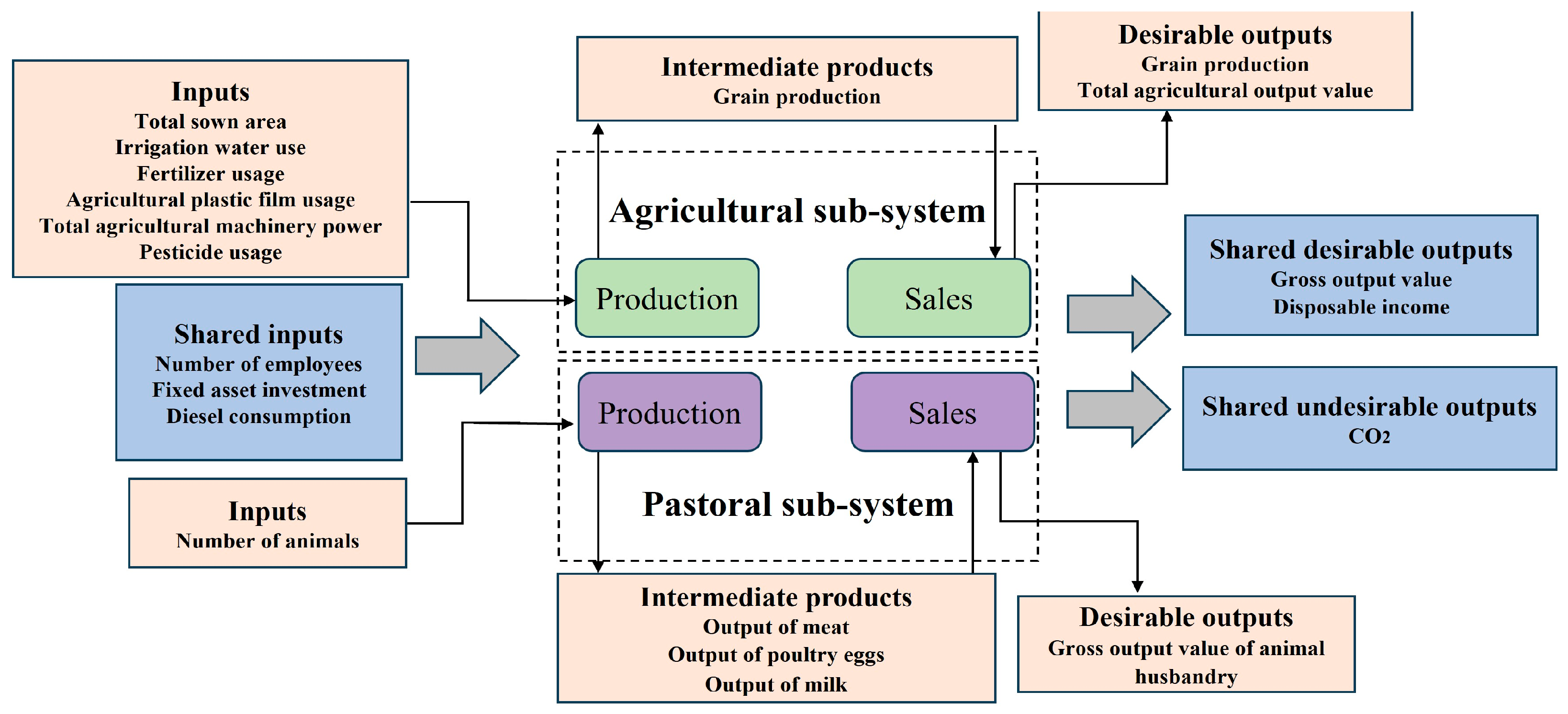
Based on existing research, this paper scientifically selects several factors. Figure 3 illustrates the inputs and outputs in agricultural and pastoral systems. In the agricultural sub-systems, inputs include “Total sown area”, “Irrigation water use”, “Fertilizer usage”, “Agricultural plastic film usage”, “Total agricultural machinery power”, and “Pesticide usage”. The desirable output is “Total agricultural output value”. “Grain production” is the intermediate product. In the pastoral sub-systems, the input is “Number of animals”. Intermediate products include “Output of meat”, “Output of poultry eggs”, and “Output of milk”. The desirable output is “Gross output value of animal husbandry”. Shared inputs include “Number of employees”, “Fixed asset investment”, and “Diesel consumption”. Shared desirable outputs are “Gross output value” and “Disposable income”. The shared undesirable output is “CO₂”. The factors mentioned above are common inputs and outputs in agricultural and pastoral systems. Decision-makers utilize these inputs to generate certain outputs, while simultaneously producing CO₂ as a byproduct. The selected data are based on the agricultural and pastoral systems of 30 provinces and cities in China from the China Statistical Yearbook 2023.

Table 5. Summary of the factors corresponding to the agricultural sub-systems.

	Total Sown Area (1000 Ha)	Irrigation Water Use (1000 Ha)	Fertilizer Usage (10,000 t)	Agricultural Plastic Film Usage (10,000 t)	Total Agricultural Machinery Power (10,000 KW)	Pesticide Usage (10,000 t)	Grain Production (10,000 t)	Total Agricultural Output Value (CNY 100 M)
Max	15,209.41	6534.69	595.31	27.9	11,530.49	10.5	7763.14	6948.30
Min	143.81	112.14	4.71	0.7	100.19	0.1	45.36	129.77
Average	5657.12	2335.14	169.21	7.91	3787.99	3.96	2284.85	2810.59
St. Dev.	4040.11	1905.58	128.16	6.62	3014.69	2.99	2012.91	1825.04

,

Table 6. Summary of the factors corresponding to the pastoral sub-systems.

	Number of Animals (10,000 Heads)	Output of Meat (10,000 t)	Output of Poultry Eggs (10,000 t)	Output of Milk (10,000 t)	Gross Output Value of Animal Husbandry (CNY 10,000)
Max	956.9	844.51	456.24	733.83	3281.67
Min	5.8	4.33	1.49	0.28	42.29
Average	338.93	309.99	115.18	129.28	1350.29
St. Dev.	297.40	222.48	131.44	183.43	910.57

and

Table 7. Summary of the shared factors.

	Number of Employees (10,000)	Fixed Asset Investment (CNY 100 M)	Diesel Consumption (10,000 t)	Gross Output Value (CNY 10,000)	Disposable Income (CNY)	CO2 (10,000 t)
Max	1602	190.6	171.4	9780.6	39,729	533.9
Min	21	0.2	1.7	172.06	12,165	5.3
Average	586.4	81.16	58.85	4160.89	20,945.03	183.31
St. Dev.	408.01	63.33	44.62	2656.97	6731.25	139.00

show the summary of the relevant factors.

Scientifically determining the proportion of various stages and factors is crucial. This paper, based on interviews with experts, determines the distribution ratios for each stage and element. In our study, the production stage and the sales stage are equally important; thus, the following equation holds: ${\sigma }_{A1}={\sigma }_{A2}={\sigma }_{P1}={\sigma }_{P1}=0.5$. In China, the contribution of the agricultural system to Gross Domestic Product is higher than that of the pastoral system. Therefore, based on experts’ recommendations, this paper determines the proportion between the agricultural and pastoral systems to be as follows: $w_A=0.6$, $w_P=0.4$. Similarly, taking experts’ recommendations into account, more shared factors should be allocated to the agricultural sub-system compared to the pastoral sub-system. The proportions of “Number of employees”, “Fixed asset investment”, and “Diesel consumption” allocated to the agricultural sub-system are 0.65, 0.55, and 0.5, respectively. Their proportions allocated to the pastoral sub-system are 0.35, 0.45, and 0.5, respectively. The proportions of “Gross output value” and “Disposable income” allocated to the agricultural sub-system are 0.7 and 0.75, respectively, which means that the proportions allocated to the pastoral sub-system are 0.3 and 0.25. The proportion of CO₂ allocated to the agricultural sub-system is 0.7, and the value allocated to the pastoral sub-system is 0.3.

4.2. Results

By applying Models (4), (8), and (12), we can obtain the evaluation results, which are reported in

Table 8. Evaluation results.

DMU	E Overall Efficiency	EA Agricultural Sub-Systems’ Efficiency	EP Pastoral Sub-Systems’ Efficiency	EAP Production Efficiency of Agricultural Sub-Systems	EAS Sales Efficiency of Agricultural Sub-Systems	EPP Production Efficiency of Pastoral Sub-Systems	EPS Sales Efficiency of Pastoral Sub-Systems
Beijing	1	1	1	1	1	1	1
Tianjin	1	1	1	1	1	1	1
Hebei	0.7535	0.6650	0.8861	0.4425	0.8876	0.8274	0.9449
Shanxi	0.7001	0.5962	0.8559	0.3753	0.8171	0.7201	0.9917
Inner Mongolia	0.7126	0.6087	0.8684	0.3446	0.8728	0.7475	0.9892
Liaoning	0.7409	0.6516	0.8749	0.4042	0.8991	0.7739	0.9759
Jilin	0.6965	0.5888	0.8579	0.3352	0.8424	0.7627	0.9532
Heilongjiang	0.7159	0.6372	0.8339	0.3617	0.9128	0.7282	0.9397
Shanghai	1	1	1	1	1	1	1
Jiangsu	1	1	1	1	1	1	1
Zhejiang	0.8317	0.7195	1	0.4391	1	1	1
Anhui	0.7434	0.6198	0.9287	0.3554	0.8843	0.8709	0.9865
Fujian	0.7933	0.6983	0.9357	0.5193	0.8773	0.8804	0.9910
Jiangxi	0.7353	0.6311	0.8914	0.3904	0.8719	0.7868	0.9961
Shandong	0.9127	0.8545	1	0.7090	1	1	1
Henan	1	1	1	1	1	1	1
Hubei	0.7992	0.7134	0.9279	0.4510	0.9758	0.8558	1
Hunan	0.8240	0.7284	0.9675	0.4909	0.9659	0.9414	0.9935
Guangdong	0.8622	0.7704	1	0.5408	1	1	1
Guangxi	0.7904	0.7341	0.8749	0.4769	0.9913	0.8036	0.9463
Hainan	0.7708	0.6815	0.9048	0.3630	1	0.8126	0.9971
Chongqing	0.7983	0.7041	0.9396	0.4855	0.9226	0.8811	0.9981
Sichuan	1	1	1	1	1	1	1
Guizhou	1	1	1	1	1	1	1
Yunnan	0.8559	0.7599	1	0.5806	0.9392	1	1
Shaanxi	0.7533	0.7025	0.8297	0.4893	0.9156	0.7386	0.9208
Gansu	0.6997	0.6132	0.8294	0.4014	0.8251	0.7001	0.9588
Qinghai	0.8944	0.9119	0.8681	1	0.8239	0.7413	0.9949
Ningxia	0.6969	0.6094	0.8283	0.3841	0.8347	0.6707	0.9859
Xinjiang	0.7220	0.6556	0.8217	0.4231	0.8881	0.7469	0.8966
Max	1	1	1	1	1	1	1
Min	0.6965	0.5888	0.8339	0.3352	0.8171	0.7201	0.9397
Average	0.8415	0.7745	0.9419	0.6026	0.9464	0.8957	0.9881

. From an overall efficiency perspective, Beijing, Tianjin, Shanghai, Jiangsu, Henan, Sichuan, and Guizhou are efficient because the values of $E_A$, $E_P$, $E_{AP}$, $E_{AS}$, $E_{PP}$, and $E_{PS}$ for them are all 1. The remaining DMUs are inefficient. Jilin’s performance is the poorest, with an efficiency score of only 0.6965, which indicates that its production process needs to be optimized. Ningxia’s efficiency value is 0.6969, ranking them second to last. It highlights that Ningxia’s production strategies need timely adjustments.

In terms of agricultural sub-system efficiency $E_A$, Beijing, Tianjin, Shanghai, Jiangsu, Henan, Sichuan, and Guizhou are efficient with an efficiency score of 1. Jilin has the poorest performance with an efficiency score of 0.5888. This indicates that there are serious production issues within Jilin’s agricultural sub-system. The values of $E_{AP}$ and $E_{AS}$ for Jilin are 0.3352 and 0.8424, respectively, which are both relatively low compared to other DMUs. Shanxi’s efficiency is 0.5888. This indicates that there are issues within the agricultural sub-system as well. The values of $E_{AP}$ and $E_{AS}$ for Shanxi are 0.3753 and 0.8171, respectively, ranking towards the lower end. For Jilin and Shanxi, the inputs are substantial, but the outputs are relatively low among the 30 DMUs, especially considering that Shanxi’s total agricultural output value is only 1288.41. This indicates that they use a considerable amount of inputs to generate few outputs, which contributes to their lower efficiency. To improve the efficiency of the agricultural sub-system, based on our results, Jilin should reduce irrigation water use by 1286.75 (1000 Ha), fertilizer usage by 194.83 (10,000 t), agricultural plastic film usage by 3.61 (10,000 t), total agricultural machinery power by 3613.46 (10,000 KW), pesticide usage by 3.90 (10,000 t), CO₂ emissions by 40.54 (10,000 tons), and diesel consumption by 26.07 (10,000 t), while increasing the total agricultural output value by 646.56 (CNY 100 M) and disposable income by 10,349.15 (CNY). Shanxi should reduce irrigation water use by 998.64 (1000 Ha), fertilizer usage by 79.98 (10,000 t), agricultural plastic film usage by 4.01 (10,000 t), total agricultural machinery power by 1103.34 (10,000 KW), pesticide usage by 1.91 (10,000 t), CO₂ emissions by 41.63 (10,000 t), and diesel consumption by 9.18 (10,000 t), while increasing the total agricultural output value by 192.73 (CNY 100 M) and disposable income by 9340.17 (CNY).

From the perspective of pastoral sub-system efficiency $E_P$, Beijing, Tianjin, Shanghai, Jiangsu, Zhejiang, Henan, Shandong, Sichuan, Guangdong, Guizhou, and Yunnan are efficient with an efficiency score of 1, which illustrates that they perform well. Xinjiang has the lowest efficiency at just 0.8217. From perspective of the production and sales stages, the values for $E_{PP}$ and $E_{PS}$ of Xinjiang are 0.7469 and 0.8966, respectively, which are significantly lower compared to other DMUs. Ningxia’s efficiency stands at 0.8283, ranking them second to last among the 30 DMUs. The values of $E_{PP}$ and $E_{PS}$ for Ningxia are 0.6707 and 0.9859, respectively, with $E_{PP}$ ranking last. This indicates that there are significant issues in its pastoral system’s production stage. For Xinjiang and Ningxia, their pastoral sub-systems’ efficiency places them at a disadvantage compared to other DMUs. From the data perspective, Xinjiang’s pastoral sub-system has a substantial input (number of animals) value of 851.3, but the desirable output value (gross output value of animal husbandry) is only 1305.28, which is low compared to that of the other DMUs. This results in low efficiency. Ningxia’s pastoral sub-system also has high input but low output levels, which contribute to its relatively low efficiency as well. To improve the efficiency of the pastoral sub-system, Xinjiang could reduce CO₂ emissions by 20.21 (10,000 t) and diesel consumption by 2.11 (10,000 t), while increasing the gross output value of animal husbandry by 717.81 (CNY 10,000) and disposable income by 474.48 (CNY). Ningxia could reduce CO₂ emissions by 9.59 (10,000 t) and diesel consumption by 6.04 (10,000 t), while increasing disposable income by 712.00 (CNY).

Generally speaking, Beijing, Tianjin, Shanghai, Jiangsu, Henan, Sichuan, and Guizhou are efficient regardless of the overall system, agricultural sub-system, or pastoral sub-system. However, there are issues in the agricultural and pastoral systems of the other DMUs.

We also compare the average efficiency across different regions. The results are shown in

Table 9. Evaluation results across different regions.

Regions		Overall Efficiency Average	Agricultural Sub-Systems’ Efficiency Average	Pastoral Sub-Systems’ Efficiency Average
North	Beijing	0.8332	0.7739	0.9221
	Tianjin
	Hebei
	Shanxi
	Inner Mongolia
Northeast	Liaoning	0.7178	0.6259	0.8556
	Jilin
	Heilongjiang
East	Shanghai	0.8802	0.8154	0.9774
	Jiangsu
	Zhejiang
	Anhui
	Fujian
	Shandong
Central	Jiangxi	0.8396	0.7682	0.9467
	Henan
	Hubei
	Hunan
South	Guangdong	0.8078	0.7286	0.9265
	Guangxi
	Hainan
Southwest	Chongqing	0.9135	0.8660	0.9849
	Sichuan
	Guizhou
	Yunnan
Northwest	Shaanxi	0.7532	0.6985	0.8354
	Gansu
	Qinghai
	Ningxia
	Xinjiang

. From the perspective of overall efficiency, the average value in the Southwest region is the highest, at 0.9135. The Northeast region has the lowest average value, at only 0.7178. From the perspective of agricultural sub-system efficiency, the Southwest region has the highest average, while the Northeast region has the lowest average. In terms of pastoral sub-system efficiency, the Southwest region has the highest average, at 0.9849, while the Northwest region has the lowest, at only 0.8354. The above analysis indicates that the agro-pastoral development in the Southwest region is relatively good, with high production efficiency, ranking first among the seven regions. In contrast, the agro-pastoral development in the Northwest and Northeast regions is more underdeveloped, with low production efficiency, thus requiring timely adjustments in production strategies and the optimization of production processes to improve efficiency.

5. Discussion

The existing literature on shared factors mainly adopts proportional distribution methods, which we do not discuss further here. This paper focuses on analyzing undesirable outputs and intermediate products.

5.1. Undesirable Outputs

This paper employs the SBM method to handle undesirable outputs. To explore the impact of undesirable outputs, we also consider the condition of ignoring undesirable outputs (IUO). In this scenario, constraints related to undesirable outputs in Model (12) should be deleted. There are no slack variables for undesirable outputs. Therefore, the objective function in Model (12) can be represented as the following Equation (14):

$$E=\min 1-{\displaystyle \sum _k{w}_k}({\displaystyle \frac{{\sigma }_{k1}}{I_k+M}}({\displaystyle \sum _{i=1}^{I_k}\frac{s_{ki}^{-}}{B_{ki}^{-}}+}{\displaystyle \sum _{m=1}^M\frac{s_{km}^{-}}{B_{km}^{-}}})-{\displaystyle \frac{{\sigma }_{k2}}{S_k+L}}({\displaystyle \sum _{l=1}^{S_k}\frac{s_{kr}^{+}}{B_{kr}^{+}}}+{\displaystyle \sum _{l=1}^L\frac{s_{kl}^{+}}{B_{kl}^{+}}}))$$

(14)

The efficiency under the IUO condition is also calculated. Figure 4 shows the comparison results of undesirable outputs under the two conditions.

Figure 4a shows the results of overall efficiency. Under the IUO condition, Beijing, Shanghai, Jiangsu, Henan, and Sichuan are efficient, all of them with an efficiency score of 1. Jilin has the poorest performance, with an efficiency score of 0.6868. This indicates that there are serious production issues within Jilin’s agricultural and pastoral systems. Tianjin, Inner Mongolia, Liaoning, Jilin, Anhui, Jiangxi, Hubei, Guangxi, Hainan, Chongqing, Guizhou, Yunnan, Shaanxi, Gansu, Qinghai, and Xinjiang exhibit significantly lower efficiencies under the IUO condition compared to those under the SBM condition. Hebei, Shanxi, Heilongjiang, Fujian, and Ningxia show higher efficiencies under the IUO compared to those under the SBM condition. The efficiency of the other DMUs remains the same under both methods.

Figure 4b reports the comparison results of the agricultural sub-system’s efficiency. Under the IUO condition, Beijing, Shanghai, Jiangsu, Henan, and Sichuan are efficient with an efficiency score of 1. Other DMUs are all inefficient. The efficiency of Jilin is merely 0.5788, which indicates that there are significant issues in the production process of Jilin’s agricultural sub-system that require further optimization. Tianjin, Inner Mongolia, Liaoning, Jilin, Anhui, Jiangxi, Hubei, Hunan, Guangxi, Chongqing, Guizhou, Yunnan, Shaanxi, and Xinjiang show lower efficiencies under the IUO compared to those under the SBM condition. Hebei, Shanxi, Heilongjiang, Fujian, Gansu, Qinghai, and Ningxia have higher efficiencies under the IUO compared to those under the SBM condition. The efficiency difference for the other DMUs under both conditions is not significant.

Figure 4c summarizes the comparative results of the pastoral sub-system’s efficiency. Under the IUO condition, Beijing, Shanghai, Jiangsu, Zhejiang, Shandong, Henan, Guangdong, Sichuan, Guizhou, and Yunnan are efficient, all of them with an efficiency score of 1. The remaining DMUs are all inefficient. Xinjing has the poorest performance, with an efficiency score of 0.8079, which indicates that there are significant issues in the production process of its pastoral sub-system. Tianjin, Hebei, Liaoning, Jilin, Heilongjiang, Jiangxi, Hubei, Guangxi, Hainan, Chongqing, Shaanxi, Gansu, Qinghai, Ningxia, and Xinjiang exhibit significantly lower efficiencies under the IUO condition compared to those under the SBM condition. Inner Mongolia, Shanxi, Anhui, Fujian, and Hunan show higher efficiencies under the IUO condition compared to those under the SBM condition. There is no significant difference in efficiency among the other DMUs under both methods.

According to the comparative results of overall efficiency, it can be observed that only 33% of the provinces and cities exhibit equal efficiency when applying the IUO method compared to the SBM method, while the remaining 67% show different efficiency values between the two methods. This indicates that the choice between the SBM method and the IUO method can result in significant differences in the computational results. Actually, it is not correct to apply the IUO approach to deal with undesirable outputs. For instance, it appears that Hebei and Heilongjiang have lower efficiencies under the SBM condition compared to the IUO condition from the perspective of overall efficiency. However, based on the data, Hebei and Heilongjiang both have high CO₂ emissions. In this case, their efficiency should be relatively lower, which supports the SBM method. Ignoring undesirable outputs would lead to an incorrect evaluation of efficiency in this case.

5.2. Intermediate Products

We utilize the free link method to handle agricultural sub-systems’ intermediate products (grain production) and pastoral sub-systems’ intermediate products (output of meat, output of poultry eggs, and output of milk). Besides this approach, Tone and Tsutsui [39] proposed another method called the fixed link. Under the fixed link method, the constraint in Model (12) corresponding to intermediate products can be represented as the following Constraint (15):

$$\begin{array}{l}{\displaystyle \sum _{j=1}^n{\lambda }_{k1}^j{z}_{kd}^j}=z_{kd}^o\\ {\displaystyle \sum _{j=1}^n{\lambda }_{k2}^j{z}_{kd}^j}=z_{kd}^o\end{array}$$

(15)

The free link is discretionary when maintaining continuity between inputs and outputs. It enables decision-makers to assess the suitability of the link by considering other DMUs. This approach is more flexible and suitable for complex network structures. The fixed link means that link activities are non-discretionary, which results in intermediate products being beyond the control of DMUs. Under the fixed link, each DMU’s input and output relationships remain fixed and do not change with variations in other DMUs. It is typically used for simpler and static network structures. The free link closely approximates real production scenarios and can flexibly adapt to various production changes. The efficiency under the fixed link is summarized in

Table 10. Results under the fixed link.

DMU	E	EA	EP
Beijing	1	1	1
Tianjin	1	1	1
Hebei	0.9118	0.8530	1
Shanxi	0.8479	0.7466	1
Inner Mongolia	0.9085	0.8475	1
Liaoning	0.8614	0.7689	1
Jilin	0.8534	0.8397	0.8739
Heilongjiang	1	1	1
Shanghai	1	1	1
Jiangsu	1	1	1
Zhejiang	0.8317	0.7195	1
Anhui	0.8055	0.7087	0.9506
Fujian	0.8211	0.7162	0.9783
Jiangxi	0.9398	0.9179	0.9726
Shandong	0.9127	0.8545	1
Henan	1	1	1
Hubei	0.8299	0.7165	1
Hunan	0.8446	0.7410	1
Guangdong	0.8622	0.7704	1
Guangxi	0.8414	0.7357	1
Hainan	0.8089	0.6815	1
Chongqing	0.9619	0.9366	1
Sichuan	1	1	1
Guizhou	1	1	1
Yunnan	0.8569	0.7614	1
Shaanxi	0.7839	0.7225	0.8761
Gansu	0.7469	0.6819	0.8443
Qinghai	0.9472	0.9119	1
Ningxia	0.9318	0.8863	1
Xinjiang	0.7501	0.6747	0.8631

.

It can be observed that Beijing, Tianjin, Heilongjiang, Shanghai, Jiangsu, Henan, Sichuan, and Guizhou are efficient both in terms of overall efficiency and at each stage’s efficiency. The agricultural sub-system’s efficiency of Beijing, Tianjin, Heilongjiang, Shanghai, Jiangsu, Henan, Sichuan, and Guizhou is 1, which means that they are highly efficient. When it comes to the efficiency of the pastoral system, Jilin, Anhui, Fujian, Jiangxi, Shaanxi, Gansu, and Xinjiang are inefficient, while the remaining DMUs are all efficient.

Figure 5 summarizes the efficiency comparison results of intermediate products under the free link and fixed link conditions.

Figure 5a shows the comparison results of overall efficiency. Hebei, Shanxi, Inner Mongolia, Liaoning, Jilin, Heilongjiang, Anhui, Fujian, Jiangxi, Hubei, Hunan, Guangxi, Hainan, Chongqing, Shaanxi, Gansu, Qinghai, Ningxia, and Xinjiang exhibit significantly higher efficiencies under the fixed link compared to that under the free link. The other DMUs show no significant difference in efficiency under both conditions. Figure 5b reports the comparison results of agricultural sub-systems’ efficiency. Hebei, Shanxi, Inner Mongolia, Liaoning, Jilin, Heilongjiang, Jiangxi, Chongqing, and Ningxia have significantly higher efficiencies under the fixed link compared to that under the free link. There is no significant difference in efficiency among the other provinces and cities. Figure 5c illustrates the comparison results of the pastoral sub-systems’ efficiency. Beijing, Tianjin, Shanghai, Jiangsu, Zhejiang, Shandong, Henan, Guangdong, Sichuan, Guizhou, and Yunnan have an efficiency of 1 under both conditions, with no difference. The other DMUs exhibit significantly higher efficiencies under the fixed link compared to that under the free link.

Overall, most DMUs show higher efficiencies under the fixed link condition compared to those under the free link condition. The reason for this gap is that the constraint corresponding to the free link is tighter than the constraint corresponding to the fixed link. The efficiency gap under the two conditions aligns with the link effect, which is discussed by Tone and Tsutsui [39]. Under the free link method, the transfer of intermediate products is unrestricted and can be freely allocated at different stages, offering high flexibility and better reflecting the resource allocation in actual production. In contrast, under the fixed link method, the transfer ratio of intermediate products is fixed, resulting in low flexibility and a potential inability to adapt to changes in the production process. Agricultural and pastoral systems often have complex network structures and numerous uncertain factors. Using the free link method can accurately reflect production activities. Therefore, the free link method we use allows decision-makers to effectively obtain efficiency values that align with actual production conditions.

6. Conclusions

Agricultural and pastoral systems, which consist of agricultural sub-systems and pastoral sub-systems, significantly impact the sustainable development of the agricultural economy. Accurately measuring the efficiencies of these systems to optimize their weak processes is currently a focal point of research. The presence of shared factors and undesirable outputs complicates efficiency evaluations.

To address this issue, the PPSs of the overall systems, agricultural sub-systems, and pastoral sub-systems were analyzed. Then, this study proposed network BAM models in the presence of shared factors and undesirable outputs for divisional systems. The network BAM model of overall efficiency was also presented. The new method was utilized to evaluate the efficiency of agricultural and pastoral systems across 30 provinces and cities in China. Based on our research findings, we provided targeted optimization strategies for some inefficient DMUs to help them improve their production efficiency. To explore the impact of undesirable outputs, the efficiency under the IUO condition was calculated. The results indicated that overlooking undesirable outputs may misestimate efficiency. To explore the impact of intermediate products, we also calculated the efficiency under the fixed link. The results indicated that the efficiency under the fixed link was significantly higher than that under the free link. Using the fixed link to handle intermediate products tended to overestimate efficiency to some extent.

The contribution of this paper lies in: 1. To assess the overall efficiency of agricultural and pastoral systems, we proposed a network BAM model that can cope with shared factors and undesirable outputs. 2. To assess the efficiency of agricultural sub-systems and pastoral sub-systems, two divisional network BAM models considering shared factors and undesirable outputs were developed.

For decision-makers, the methodology presented in this study can be utilized to assess the efficiency of agricultural and pastoral systems, thereby providing support for the optimization of these systems. Provinces with relatively low efficiency in agricultural and pastoral systems, such as Shanxi, Xinjiang, and Ningxia, can improve their performance by reducing the amount of irrigation water use, fertilizer usage, agricultural plastic film usage, total agricultural machinery power, pesticide usage, CO₂ emissions, and diesel consumption, while also increasing total agricultural output value and disposable income. Although the method proposed in this paper can assess the efficiency of agricultural and pastoral systems with shared factors and undesirable outputs, it still has limitations. Dual-role factors, such as research and development expenses, which can play both the input and output roles simultaneously, were overlooked in our research [40]. In future research, scholars can incorporate dual-role factors into the models presented here to evaluate the efficiency of more complex agricultural and pastoral systems. Scientifically determining the proportion of various elements is of great significance, and future research can focus on methods for determining element distribution ratios.

References

1. Martinsson, E.; Hansson, H.; Mittenzwei, K.; Storm, H. Evaluating environmental effects of adopting automatic milking systems on Norwegian dairy farms. Eur. Rev. Agric. Econ. 2024, 51, 128–156. [Google Scholar] [CrossRef]
2. Sidhoum, A.; Mennig, P.; Sauer, J. Do agri-environment measures help improve environmental and economic efficiency? Evidence from Bavarian dairy farmers. Eur. Rev. Agric. Econ. 2023, 50, 918–953. [Google Scholar] [CrossRef]
3. Chen, Y.F.; Miao, J.F.; Zhu, Z.T. Measuring green total factor productivity of China’s agricultural sector: A three-stage SBM-DEA model with non-point source pollution and CO2 emissions. J. Clean. Prod. 2021, 318, 128543. [Google Scholar] [CrossRef]
4. Manogna, R.L.; Aswini, K.M. Agricultural production efficiency of Indian states: Evidence from data envelopment analysis. Int. J. Financ. Econ. 2022, 27, 4244–4255. [Google Scholar]
5. Villa, G.; Lozano, S. A shared-input integer network DEA approach linking football teams’ wages and market values. Omega 2024, 125, 103021. [Google Scholar] [CrossRef]
6. Charnes, A.; Cooper, W.W.; Rhodes, E. Measuring the efficiency of decision making units. Eur. J. Oper. Res. 1978, 2, 429–444. [Google Scholar] [CrossRef]
7. Cooper, W.W.; Park, K.S.; Pastor, J.T. RAM: A Range adjusted measure of inefficiency for use with additive models, and relations to other models and measures in DEA. J. Prod. Anal. 1999, 11, 5–42. [Google Scholar] [CrossRef]
8. Ma, C.; Ren, J.; Chen, C. Assessing the logistics industry efficiency with a modified range adjusted measure. Sci. Rep. 2024, 14, 17653. [Google Scholar] [CrossRef]
9. Cooper, W.W.; Pastor, J.T.; Borras, F.; Aparicio, J.; Pastor, D. BAM: A bounded adjusted measure of efficiency for use with bounded additive models. J. Prod. Anal. 2011, 35, 85–94. [Google Scholar] [CrossRef]
10. Chen, Y.; Du, J.; David Shermanc, H.; Zhu, J. DEA model with shared resource sand efficiency decomposition. Eur. J. Oper. Res. 2010, 207, 339–349. [Google Scholar] [CrossRef]
11. Zhang, Z.; Wang, Z.; Zhu, Y. Optimal path selection of innovation resource allocation in China’s regions with shared inputs. Econ. Res. Istraz. 2021, 35, 1457–1480. [Google Scholar] [CrossRef]
12. Toloo, M.; Emrouznejad, A.; Moreno, P. A linear relational DEA model to evaluate two-stage processes with shared inputs. Comput. Appl. Math. 2017, 36, 45–61. [Google Scholar] [CrossRef]
13. Zhu, W.; Zhang, Q.; Wang, H. Fixed costs and shared resources allocation in two-stage network DEA. Ann. Oper. Res. 2017, 278, 177–194. [Google Scholar] [CrossRef]
14. Zhao, H.H.; Liu, Y.; Li, J.; Guo, X.G.; Gui, H.J. Chinese provincial difference in the efficiency of universities scientific and technological activities based on dea with shared input. Math. Probl. Eng. 2022, 2022, 8319498. [Google Scholar] [CrossRef]
15. Wu, J.; Xiong, B.; An, Q.; Sun, J.; Wu, H. Total-factor energy efficiency evaluation of Chinese industry by using two-stage DEA model with shared inputs. Ann. Oper. Res. 2015, 255, 257–276. [Google Scholar] [CrossRef]
16. Wang, D.W.; Zhao, L.L.; Yang, F.; Chen, K.H. Performance evaluation of the Chinese high-tech industry: A two-stage DEA approach with feedback and shared resource. J. Ind. Manag. Optim. 2022, 18, 3315–3338. [Google Scholar] [CrossRef]
17. Chen, H.; Lin, H.; Zou, W. Research on the Regional differences and influencing factors of the innovation efficiency of China’s high-tech industries: Based on a shared inputs two-stage network DEA. Sustainability 2020, 12, 3284. [Google Scholar] [CrossRef]
18. Lin, S.W.; Lu, W.M. Discretionary investment managers evaluation in pension fund: Shared input dynamic network DEA approach. Omega 2024, 127, 103107. [Google Scholar] [CrossRef]
19. An, Q.X.; Wen, Y.; Ding, T.; Li, Y.L. Resource sharing and payoff allocation in a three-stage system: Integrating network DEA with the Shapley value method. Omega 2019, 85, 16–25. [Google Scholar] [CrossRef]
20. Shabani, P.; Shirazi, M.A. Performance evaluation of commercial bank branches in dynamic competitive conditions: A network DEA model with serial and cross-shared resources. J. Econ. Stud. 2024, 51, 1–23. [Google Scholar] [CrossRef]
21. He, K.; Zhu, N. Efficiency evaluation of Chinese provincial industry systems: A dynamic two-stage slacks-based measure with shared inputs. J. Ind. Manag. Optim. 2023, 19, 4959–4988. [Google Scholar] [CrossRef]
22. Chen, X.; Liu, X.; Gong, Z.; Xie, J. Three-stage super-efficiency DEA models based on the cooperative game and its application on the R&D green innovation of the Chinese high-tech industry. Comput. Ind. Eng. 2021, 156, 107234. [Google Scholar]
23. Liu, W.B.; Meng, W.; Li, X.X.; Zhang, D.Q. DEA models with undesirable inputs and outputs. Ann. Oper. Res. 2010, 173, 177–194. [Google Scholar] [CrossRef]
24. Izadikhah, M.; Khoshroo, A. Energy management in crop production using a novel fuzzy data envelopment analysis model. RAIRO Oper. Res. 2018, 52, 595–617. [Google Scholar] [CrossRef]
25. Fare, R.; Grosskopf, S.; Lovell, C.A.K.; Pasurka, C. Multiple productivity comparisons when some outputs are undesirable: A nonparametric approach. Rev. Econ. Stat. 1989, 71, 90–98. [Google Scholar] [CrossRef]
26. Roshdi, I.; Hasannasab, M.; Margaritis, D.; Rouse, P. Generalized weak disposability and efficiency measurement in environmental technologies. Eur. J. Oper. Res. 2018, 266, 1000–1012. [Google Scholar] [CrossRef]
27. Li, F.; Deng, L.; Li, L.; Cheng, Z.; Yu, H. A two-stage model for monitoring the green supplier performance considering dual-role and undesirable factors. Asia Pac. J. Mark. Logist. 2019, 32, 253–280. [Google Scholar] [CrossRef]
28. Chen, X.; Wu, G.; Li, D. Efficiency measure on the truck restriction policy in China: A non-radial data envelopment model. Transp. Res. Part A Policy Pract. 2019, 129, 140–154. [Google Scholar] [CrossRef]
29. Mirhedayatian, S.M.; Azadi, M.; Saen, R.F. A novel network data envelopment analysis model for evaluating green supply chain management. Int. J. Prod. Econ. 2014, 147, 544–554. [Google Scholar] [CrossRef]
30. Chen, X.D.; Miao, Z.; Wang, K.L.; Sun, C.W. Assessing eco-performance of transport sector: Approach framework, static efficiency and dynamic evolution. Transp. Res. Part D Transp. Environ. 2020, 85, 102414. [Google Scholar] [CrossRef]
31. Rashidi, K.; Saen, R.F. Measuring eco-efficiency based on green indicators and potentials in energy saving and undesirable output abatement. Energy Econ. 2015, 50, 18–26. [Google Scholar] [CrossRef]
32. Pastor, J.T.; Aparicio, J.; Alcaraz, J.; Vidal, F.; Pastor, D. An enhanced BAM for unbounded or partially bounded CRS additive models. Omega 2015, 56, 16–24. [Google Scholar] [CrossRef]
33. Khoshroo, A.; Izadikhah, M.; Emrouznejad, A. Energy efficiency and congestion considering data envelopment analysis and bounded adjusted measure: A case of tomato production. J. Clean. Prod. 2021, 328, 129639. [Google Scholar] [CrossRef]
34. Ma, C.Y.; Ren, J.W.; Chen, C.H. A network bounded adjusted measure for dealing with dual-role factors and undesirable outputs in multi-stage systems. Int. J. Syst. Sci. Oper. 2024, 11, 2374290. [Google Scholar] [CrossRef]
35. Wu, G.; Zhu, C.X.; Jiang, J.H.; Chen, X.D. Fuel consumption, vehicle quantities, and total factor inefficiency in China. Chin. J. Popul. Resour. Environ. 2022, 20, 147–158. [Google Scholar] [CrossRef]
36. Zhang, S.; Li, X.; Nie, Z.; Wang, Y.; Li, D.; Chen, X.; Liu, Y.; Pang, J. The significance of agricultural modernization development for agricultural carbon emission efficiency in China. Agriculture 2024, 14, 939. [Google Scholar] [CrossRef]
37. Guo, C.; Zhang, R.; Zou, Y. The efficiency of China’s agricultural circular economy and its influencing factors under the rural revitalization strategy: A DEA–Malmquist–Tobit approach. Agriculture 2023, 13, 1454. [Google Scholar] [CrossRef]
38. Nandy, A.; Singh, P.K. Application of fuzzy DEA and machine learning algorithms in efficiency estimation of paddy producers of rural Eastern India. Benchmarking 2021, 28, 229–248. [Google Scholar] [CrossRef]
39. Tone, K.; Tsutsui, M. Network DEA: A slacks-based measure approach. Eur. J. Oper. Res. 2009, 197, 243–252. [Google Scholar] [CrossRef]
40. Ebrahimi, B.; Tavana, M.; Kleine, A.; Dellnitz, A. An epsilon-based data envelopment analysis approach for solving performance measurement problems with interval and ordinal dual-role factors. Or Spectr. 2021, 43, 1103–1124. [Google Scholar] [CrossRef]
Figure 1. The parallel structure of an agricultural and pastoral system.
Agriculture 15 00535 g001
Figure 2. Production and sales stages within an agricultural and pastoral system.
Agriculture 15 00535 g002
Figure 3. The inputs and outputs in the agricultural and pastoral systems.
Agriculture 15 00535 g003
Figure 4. Comparison results: (a) overall efficiency; (b) agricultural sub-system efficiency; (c) pastoral sub-system efficiency.
Agriculture 15 00535 g004
Figure 5. Comparison results: (a) overall efficiency; (b) agricultural sub-system’s efficiency; (c) pastoral sub-system’s efficiency.
Agriculture 15 00535 g005