Modeling the Performance of a Continuous Durum Wheat Cropping System in a Mediterranean Environment: Carbon and Water Footprint at Different Sowing Dates, Under Rainfed and Irrigated Water Regimes

Abstract

This study evaluates the environmental impacts and productivity of a continuous durum wheat cropping system under three sowing dates and two water regimes, i.e., rainfed and irrigation at flowering in the Mediterranean context, specifically in the Capitanata plain of Apulia, Italy. AquaCrop-GIS was employed to model the yield response of durum wheat on the different sowing dates (15 October, 1 November, and 15 November) and with different water management practices. In addition, the Carbon and Water Footprint (CWFP) tool was used to quantify the environmental impacts in terms of greenhouse gas emissions and water use, including green, blue, and total water components. Results indicated that the total greenhouse gas emissions (CO₂_eq) from wheat production averaged 1201.3 kg CO₂_eq ha⁻¹, with fertilization, in particular the application of ammonium nitrate and urea, being the main contributor. Soil management practices contributed 362.9 kg CO₂_eq ha⁻¹. Early-November sowing achieved the highest productivity, 5573 kg ha⁻¹ under the rainfed option and 5722 kg ha⁻¹ under irrigated management, while mid-November sowing resulted in lower yields and 21% higher CO₂_eq emissions per kilogram of grain compared to early November. Water Footprint analysis revealed that early-November sowing had the highest green water demand, with negligible differences in blue water use between sowing dates. Overall, the integration of these data showed that optimizing sowing dates and irrigation practices can significantly improve yields and reduce environmental impacts.

1. Introduction

Wheat production is crucial for feeding the global population and represents one of the most important agricultural systems [1]. The production of Mediterranean basin accounts for 60% of the world production of durum wheat [2], which is traditionally grown under rainfed conditions using conventional tillage [3]. With 16 million hectares and a yield of 38 million tons annually, durum wheat is one of the most cultivated cereals in the Mediterranean [3,4]. The demand for wheat is expected to increase by 60% by 2050 to meet the needs of a growing global population, projected to reach nine billion [5]. However, climate change poses significant challenges to durum wheat production, including variability in yield and quality due to the impacts of climate change [6]. The main producers of durum wheat in Europe are Italy, Greece, and Spain, which together account for about 80% of the total EU production. Italian wheat production in 2020 covered an area of 1.23 Mha and a yield of 3,849,384 tons of grain [7].

However, durum wheat production is strongly influenced by environmental and climatic factors, in particular water availability and high temperatures [8,9]. This is particularly critical in the Mediterranean region, which faces harsh climatic conditions and freshwater scarcity. This highlights the need for environmental awareness to achieve resource efficiency and increase ecosystem welfare and quality [10]. Cereal production, while vital for human nutrition, often comes with environmental consequences that threaten biodiversity and ecosystem functions [11]. Cereal crops contribute to about 35% of human caloric intake [12], yet their cultivation is associated with practices that harm the environment by altering water resources and climatic conditions [13,14]. Furthermore, cereals are often grown in industrialized monocultures, which are known to require large amounts of pesticides, fertilizers, and fossil fuels [15,16].

To mitigate these impacts, conventional farming practices must evolve to incorporate eco-design and circular economy principles, enhanced by renewable energy sources [17,18]. This is even more applicable to agricultural production, which is now widely considered to be the main cause of environmental and human health degradation [19], due to the use of the following: (a) large amounts of water for irrigation, contributing to the depletion of water resources; (b) chemical fertilizers and pesticides, the production and use of which involves the consumption of primary energy resources and generates air, water, and soil pollutants and health problems; and (c) fossil fuels, which are considered responsible for the extraction of primary energy resources and the emission of greenhouse gasses (GHG) as a result of their production and combustion.

The Mediterranean climate is characterized by inter-annual and seasonal variability in precipitation, as well as frequent heat stress periods, which often lead to water-deficit situations during the most sensitive stages of the wheat growth cycle, significantly reducing productivity [20]. This circumstance tends to be aggravated by climate change [21], contributing to the unpredictability of productive responses and the instability of a sector already weakened by income gaps and fluctuations. To address the constraints in Mediterranean wheat production, specific agronomic practices can stabilize and even increase yields, ensuring better water use efficiency and higher grain quality. Several studies [22,23,24,25,26] highlight the potential of these practices, including the provision of additional irrigation, as discussed by [27,28]. Moreover, many studies have explored the application of efficiency and productivity indicators for water and nutrient use under varying water regimes [23,29,30,31,32,33].

Water productivity values, expressed as the ratio between the product obtained (grain yield) and the input used (crop evapotranspiration or the volume of irrigation water), serve as indicators for assessing the impact of various options on resource productivity and farm outcomes [34,35]. Furthermore, the assessment of the impact of human consumption on freshwater resources used in industrial and/or agricultural processes, called “virtual water”, has been carried out using the Water Footprint (WFP) concept [36]. The WFP is a tool commonly used to analyze water management, and the WF of a product is defined as the volume of freshwater used to produce that product and should be measured along the entire supply chain. This is more commonly expressed as the volume of water per unit of product (m³ t⁻¹) [37].

Mekonnen and Hoekstra [37] describe the concept of blue, gray, and green water. Blue WFP measures the amount of available water that is consumed in a given period and therefore not immediately returned to the catchment; gray WFP of a process step is an indicator of the degree of freshwater pollution associated with it and is defined as the volume of freshwater required to assimilate the pollutant load; green WFP is an indicator of human water use and refers to precipitation that does not runoff or recharge the groundwater, but is stored in the soil or temporarily remains on the soil surface or vegetation. The sum of these three components gives the total WFP. In agriculture, many studies emphasize the importance of responsible use of water resources [38]. The WFP indicator [39] is a tool that provides interesting information for policy makers [40] and economists and is useful for water management. Rodriguez et al. [41] highlighted the importance of agricultural practices, such as irrigation and fertilization, on crop WFP. However, the WFP indicator should be considered as a partial tool that can be used together with other indicators to allow a deeper look at integrated policies [42]. Global water and carbon energy cycles are inextricably linked [43]. Scientific evidence has shown that the climate is changing rapidly, mainly due to increasing greenhouse gas emissions [44] resulting from various human activities, including agriculture [45]. The carbon footprint (CFP) of a product corresponds to the greenhouse gas emissions associated with the life cycle of that product (LCA), calculated from the beginning, represented by the extraction of raw materials (cradle), to the consumption of the final product (grave). However, the LCA can be interrupted at intermediate points, such as the harvesting of wheat grain (gate) [46,47]. It is usually expressed as the amount of CO₂_eq for a previously defined unit of measurement. Thus, the CFP is a part of the Life Cycle Assessment (LCA) methodology, which is already applied in many production sectors, including food analyses. It has been used in the cereals sector since the 2000s [48] and has contributed significantly to improving information on the environmental impacts of cereal production systems. In contrast to LCA, which is more complex and linked to a broader range of environmental impact categories, these indicators are more easily understood by the media and the organized retail trade.

This study aimed to comprehensively evaluate the impact of the most common agricultural practices on conventional wheat production in the province of Foggia, Southern Italy, under Mediterranean climatic conditions. The AquaCrop-GIS software (ver. 2.1) [49] was used to simulate the yield response of durum wheat to different sowing dates (15 October, 1 November, and 15 November) and water management practices, including rainfed conditions and supplemental irrigation during the flowering stage. Moreover, the environmental impact of these agricultural practices was quantified by assessing their CFP and WFP using a free tool designed to estimate the environmental impact of durum wheat production (CWFP application) [50]. Through this tool, the greenhouse gas emissions associated with the life cycle of durum wheat production were determined, from the extraction of raw materials necessary to produce agro-technological inputs to their application in the field and the harvesting of the grain. Water consumption was also assessed, considering both blue and green water and the associated footprints. Consequently, the analysis of trade-offs between the productive performance of durum wheat cultivation and environmental sustainability was conducted using AquaCrop-GIS and CWFP. This included examining how different cropping options—such as sowing dates and irrigation—combined with climatic variables and soil types at specific cultivation sites, could balance performance and sustainability within traditional durum wheat production.

2. Materials and Methods

The research approach followed a hierarchical scale, where each numerical level played a critical role in guiding the subsequent analysis. Starting with an examination of the production context, customized simulation scenarios were developed to assess the performance of durum wheat cultivation in relation to environmental impacts. The results of these simulations were then analyzed through appropriate numerical methods to extract meaningful insights (Figure 1).

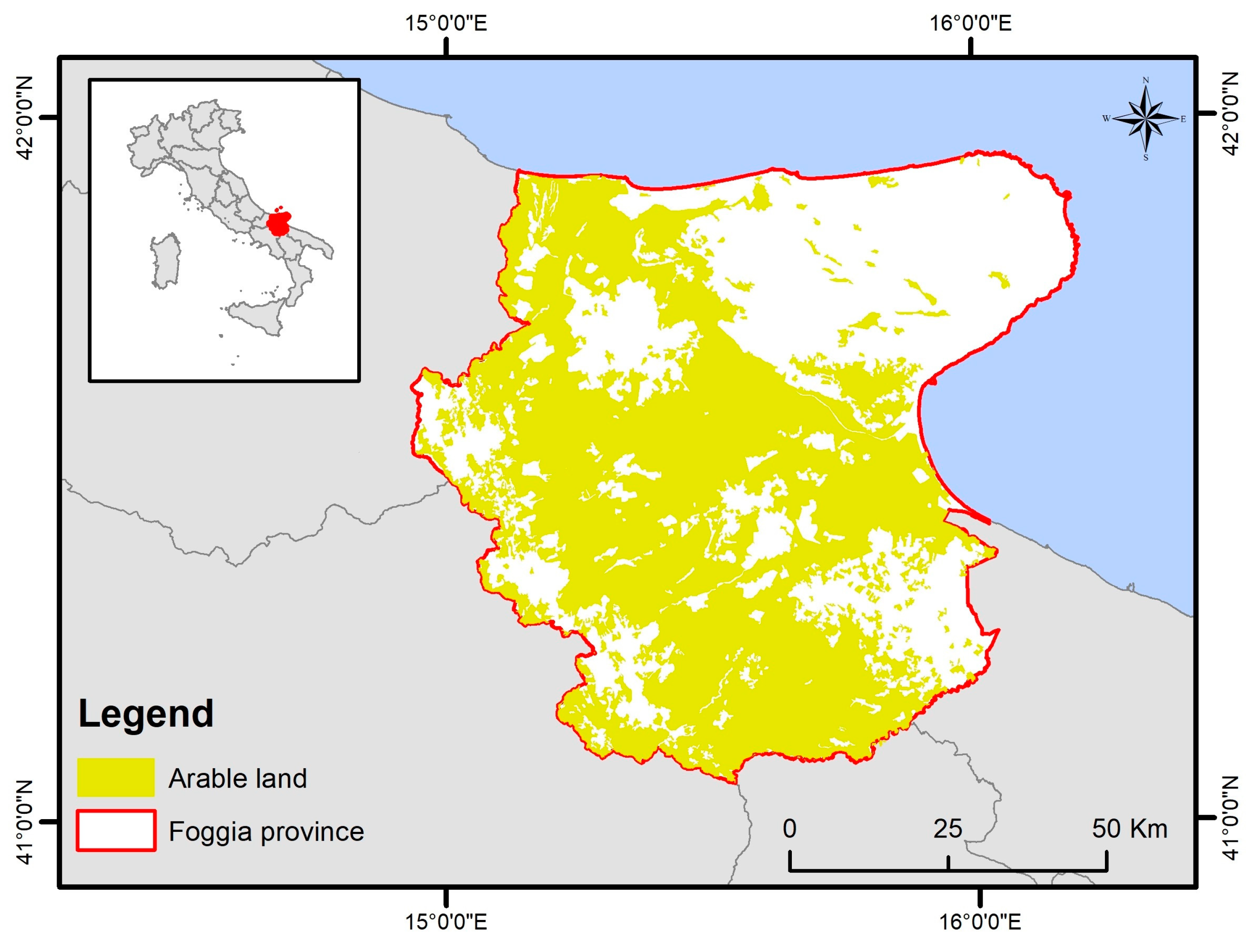
2.1. Context of the Investigated Scenarios

Simulation scenarios were based on actual practices followed by farmers in the province of Foggia, also known as Capitanata, in the Apulia region (41°27′ N, 15°33′ E, 76 m a.s.l.: Figure 2). This area is Italy’s leading producer of durum wheat, accounting for 38% of the total cultivated land dedicated to this crop [51]. The extension of arable land is represented in Figure 2 according to the Regional Land Use Cover database [52]. Durum wheat is grown in continuous cropping systems, with sowing typically occurring between mid-October and mid-November.

In this agricultural area, crop management involves land preparation for sowing, which includes summer plowing followed by two harrowing. These practices are necessary to renew soil fertility in the upper layers during plowing (by overturning soil clods to a depth of 0.45 m, which is in the zone not affected by organic matter degradation, as well as bringing weed seeds to the surface for appropriate herbicide treatment) and to facilitate the breakdown of large clods produced during the plowing phase using a disk harrow. Just before sowing, the soil is finely tilled with a rotary tiller to prepare the seedbed, preceded by the application of nitrogen fertilizer as a starter for the development of durum wheat seedlings. A second nitrogen application is provided during the vegetative phase (the first half of March) to promote tillering and growth and to ensure an adequate protein content in the grains of the crop. Grain is harvested using a combined harvester with straw either left on the ground or collected as bales. In Capitanata, durum wheat is typically grown under rainfed conditions; though in particularly dry years, farmers may resort to irrigation until the flowering stage, with 1–2 irrigations aimed at stabilizing yields rather than increasing productivity. The conventional tillage system described above is used by most farms cultivating durum wheat in continuous cropping systems, covering approximately 96% of the area dedicated to this crop [7].

2.2. Simulation Setup

To simulate durum wheat production under continuous cropping in Capitanata, AquaCrop (version 2.1, GIS extension) was utilized. This software allows for the simulation of multiple scenarios, including variations in crop type, irrigation management, soil characteristics, and climatic conditions, with outputs tailored to specific input combinations. Developed by the Food and Agriculture Organization (FAO) [53,54], AquaCrop predicts crop productivity, water demand, and water use efficiency under water-limited conditions [55]. Its framework is based on the principles of crop yield response to water [56].

AquaCrop has been applied to different scenarios such as rainfed conditions, deficit irrigation, full water supply, and on-farm water management strategies, all aimed at improving water efficiency in agriculture [57]. The model balances accuracy, simplicity, and robustness, making its parameters intuitive and transparent for users [54]. AquaCrop formalizes processes such as soil water dynamics, canopy development, phenology, plant growth, and yield formation, accounting for both potential growth and stress-modulated growth. Thermal and water stresses are modeled as functions of climatic factors, including temperature, rainfall, evapotranspiration, and atmospheric CO₂ concentrations [58]. Irrigation management in AquaCrop affects soil water balance, crop management, and yield [55]. Water is added to the soil reservoir through rainfall and irrigation. In cases of high rainfall intensity, some of the precipitation may be lost to surface runoff, with only a fraction infiltrating into the soil. The infiltrated water is not always retained in the root zone. If the root zone becomes excessively wet, some soil water will percolate out of the root zone, leading to deep percolation losses. In addition, water can move upwards to the root zone by capillary upwelling. Processes such as soil water evaporation and crop transpiration remove water from the reservoir. In terms of water use by the cropping systems, the daily crop transpiration (Tr_i, mm day⁻¹) is distinguished from the daily reference evapotranspiration (ET0i; mm day⁻¹) and are influenced by the adjusted canopy cover (CC*) as expressed below:

$${\mathrm{T}\mathrm{r}}_{\mathrm{i}}={\mathrm{k}}_{\mathrm{s}} \mathrm{\ast } \mathrm{C}\mathrm{C}\mathrm{*} \mathrm{\ast } {\mathrm{k}}_{\mathrm{c}}\mathrm{T}\mathrm{r}\mathrm{x} \mathrm{\ast } \mathrm{E}\mathrm{T}0$$

(1)

where k_S denotes the soil water stress coefficient, k_cTrx represents the coefficient for maximum crop transpiration, and CC* refers to the actual green canopy cover, adjusted for micro-advective effects.

The daily above-ground biomass (TDM, t ha⁻¹) is computed using Tri and the water productivity is normalized for ET0i (WP*, g/m; [59] as follows:

$$\mathrm{T}\mathrm{D}\mathrm{M}=\mathrm{W}\mathrm{P}\mathrm{*} \mathrm{\ast } {\sum }_{\mathrm{i}=1}^{\mathrm{n}}{\displaystyle \frac{{\mathrm{T}\mathrm{r}}_{\mathrm{i}}}{{\mathrm{E}\mathrm{T}0}_{\mathrm{i}}}}$$

(2)

Finally, dry yield (Y, t ha⁻¹) is estimated at maturity from TDM and harvest index (HI, %) according to the following equation:

$$\mathrm{Y}=\mathrm{H}\mathrm{I} \mathrm{\ast } \mathrm{T}\mathrm{D}\mathrm{M}$$

(3)

Soil water stress affects canopy development, root zone expansion, induces stomatal closure, reduces crop transpiration rates, affects pollination success, alters yield index, and can induce premature canopy senescence. These processes are affected by soil water stress when water stored in the root zone falls below certain thresholds. These thresholds are defined as root zone depletion, a fraction of the total available water. Simulations with AquaCrop covered scenarios produced in several combinations, using three sowing dates (15 October, 1 November, and 15 November) coupled with two irrigation scenarios, namely, rainfed conditions and water supply at the flowering stage, with a maximum of two irrigations and a total irrigation volume not exceeding 60 mm. The behavior of the cropping system is strongly influenced by the pedo-climatic conditions of the cropping context. Therefore, to obtain the most reliable simulations, the soil characteristics were diversified in relation to the soil properties and typical climatic trends of the area under study. Specifically, using the Harmonised World Soil Database [60], 25 different soils with different characteristics were classified.

The fraction (%) of sand, silt, and clay, hydraulic conductivity (Ksat; mm day⁻¹), soil depth (cm), bulk density (BD, g cm⁻³), and Total Organic Carbon (TOC; %) were identified by intersecting the soil database with climatic cells from the Agri4Cast database. The hydraulic characteristics of the soil used in the simulated fields, such as field capacity (FC, m³ m⁻³), wilting point (WP, m³ m⁻³), and soil–plant available water (PAW, mm), were directly estimated by AquaCrop-Windows (ver. 7.0) based on the sand, silt, and clay fractions input for the different soils. The values obtained were then set in AquaCrop-GIS to perform the various simulation scenarios. The Harmonised World Soil Database version 2.0 is a unique global soil inventory that provides information on the morphological, chemical, and physical properties of soils at a resolution of about 1 km. For the climatic characterization, the weather data used in the simulation procedure were obtained from the Agri4Cast database [61]. This is a part of the Crop Growth Monitoring System developed by the Joint Research Centre and contains meteorological data from weather stations interpolated on a 25 × 25 km grid, available daily since 1975. The maximum, average, and minimum air temperature (T, °C), precipitation (P, mm/d), potential evaporation from a free water surface (E, mm/d), potential evaporation from a moist bare soil surface (ES, mm/d), and potential evapotranspiration from a reference crop canopy (ET0, mm/d) were derived from the weather data. Fifteen grid cells covered the reference area, and the data covered a 10-year period, from 1 January 2013 to 31 December 2023. Using the ArcGIS v.10.2 software, the two databases were intersected, resulting in 74 different combinations of soil types and climatic conditions. The pedo-climatic characterization thus obtained was complemented by durum wheat specifications modeled on the inputs required by the simulation model. For durum wheat, the coefficients and parameters required to reproduce its phenotype in AquaCrop were derived from previous modeling carried out in the same growing area as this research has justified [62]. The simulations, in the different combinations (sowing date × irrigation management × weather × soil; 432 in total), covered a 10-year continuous cropping period (from 1 January 2013 to 31 December 2023). The output variables collected from the AquaCrop outputs concerned grain production, dry biomass at harvest, seasonal ET0, accumulated growing degree days (GDD; °C), and crop growing length averaged over the cropping years.

2.3. Environmental Performance Assessment

The environmental performance of the cropping system was formalized using the Carbon and Water Footprint tool [63]. This tool quantifies greenhouse gas emissions (expressed as CO₂_eq) and water use (blue and green components) in durum wheat cultivation within the Mediterranean environment. CWFP development follows core LCA steps, including defining scope, objectives, system boundaries, input material flows, impact allocation, functional unit, and environmental footprint. The tool’s design focuses on user accessibility, featuring an intuitive interface that integrates key soil and crop management practices. For each selected option, CWFP calculates environmental impacts using processes implemented in SimaPro (version 8). The tool uses a “cradle-to-gate” analysis, which confines the system within the farm boundaries and requires data from sowing to harvesting, accounting for the impacts from raw material extraction, agro-input production, and their application in the field. Material and energy flows include various machinery, equipment, fertilizers, and pesticides relevant to durum wheat cropping systems in the Mediterranean context.

For each agricultural operation provided by the user, including soil tillage (e.g., plowing, disking harrowing), fertilization (either organic or chemical), use of plant protection products, and other cropping system operations (e.g., conventional sowing, no-till sowing, harvesting), the CWFP tool estimates both direct GHG emissions and indirect GHG emissions. Direct emissions refer to those occurring directly from cropping system management, such as GHG emissions from fuel combustion in tractors or N₂O release from fertilizers applied in the field. Indirect emissions are those associated with the production of agro-inputs, such as fertilizers, fuel, pesticides, and machinery. The quantification of GHG emissions for each operation i is performed as follows:

$${\mathrm{G}\mathrm{H}\mathrm{G}}_{\mathrm{i}}={\sum }_{\mathrm{j}=1}^{\mathrm{n}}\left(\mathrm{A}\mathrm{F}\mathrm{a}\mathrm{g},\mathrm{j}\right) \mathrm{\ast } \mathrm{E}\mathrm{F}\mathrm{a}\mathrm{g},\mathrm{j}$$

(4)

where AFag,j is the amount of agro-input j used in operation i, EFag,j is the emission factor of the gas j emitted per unit of agro-input, and ∑ (from j = 1 to n) accounts for the emissions from all gasses j.

The sum of GHGi emissions from every operation across the entire cropping system provides the total GHG emissions from the extraction of raw materials, their application in the field, to their harvest.

The material and energy flows responsible for direct and indirect GHG emissions are automatically accounted for by the CWFP tool. This calculation is based on the specific operations selected and the amounts applied per ha of cultivated area. For example, the tool considers the number of passes performed for soil tillage operations or the amount of fertilizer applied (in kg). These flows are quantified with reference to the processes and emission factors reported in the ECOINVENT (v.3) database [64].

The quantification of the environmental consequences of a given cropping scenario in terms of CO₂ equivalent (CO₂_eq; kg) emissions in the CWFP tool is performed following the ILCD 2011 Midpoint [65], as follows:

$${\mathrm{C}\mathrm{O}}_2\_\mathrm{e}\mathrm{q}=\sum _{\mathrm{j}}\left(\sum _{\mathrm{i}}\left(\mathrm{G}\mathrm{H}\mathrm{G}\mathrm{i}\mathrm{j} \mathrm{\ast } \mathrm{G}\mathrm{W}\mathrm{P}\mathrm{i}\right)\right)$$

(5)

where GHGij represents the amount of gas type i during operation j, GWPi is the Global Warming Potential of gas i, ∑i accounts for the GHGs emitted during a specific operation, and ∑j sums the GHG emissions across all management operations performed throughout the cropping system

Since the default soil and crop management options in CWFP may not cover all potential farmer practices, algorithms were developed to estimate fuel consumption based on tractor speed and load force [66] for alternative soil and crop scenarios not included in the default software options. Once the fuel consumption for non-default operations in CWFP is calculated, specifying the number of passes per hectare, the tool estimates the direct and indirect CO₂_eq emissions as per Equations (4) and (5). The functional unit of one hectare of cultivated soil simplifies the impact assessment, returning environmental impacts related to GHG emissions per hectare of soil (kg CO₂_eq ha⁻¹) and blue water usage (m³ ha⁻¹). In the same way as CO₂_eq, CWFP calculates the amount of blue water indirectly used by the cropping system. Blue water refers to freshwater resources stored in rivers, lakes, and groundwater. Indirect blue water accounts for the water used in the supply chain, specifically, the water consumed during the production, processing, and transportation of agro-inputs, such as fertilizers, pesticides, and machinery, before they are applied in the field [67]. The estimation of the amount of blue water is automated in CWFP along with CO₂_eq, once the type of agricultural operation/agro-input applied and the corresponding quantities are specified, referring to the ECOINVENT database. Recognizing the importance of crop residues left on the soil as a by-product, as required by UNI EN ISO LCA standards, the user is prompted to input straw removal data (kg ha⁻¹). In the absence of such data, CWFP uses algorithms based on IPCC [68] to estimate straw and root left on the soil based on grain yield as follows:

$$\mathrm{R}\mathrm{f}\mathrm{r}={\mathrm{R}\mathrm{a}\mathrm{g}}_{\mathrm{t}} \mathrm{\ast } \left(1-{\mathrm{F}\mathrm{r}\mathrm{a}\mathrm{c}}_{\mathrm{r}\mathrm{e}\mathrm{m}\mathrm{o}\mathrm{v}\mathrm{e}\left(\mathrm{t}\right)}\right)+{\mathrm{R}\mathrm{b}\mathrm{g}}_{\mathrm{t}}$$

(6)

where Rfr (kg ha⁻¹) is the crop residue returned to soil, Rag_t is the ratio of above-ground residues dry matter (kg ha⁻¹), Frac_remove(t) is the fraction crop residues removed from soil, and Rbg_t is the ratio of below-ground residues to harvested yield (kg ha⁻¹). Rag_t is determined as follows:

$${\mathrm{R}\mathrm{a}\mathrm{g}}_{\mathrm{t}}={\displaystyle \frac{\mathrm{A}\mathrm{G}\mathrm{B}}{\mathrm{G}\mathrm{Y}}} \mathrm{\ast } \mathrm{G}\mathrm{Y}$$

(7)

where AGB is the above-ground dry biomass (kg ha⁻¹), and GY is the yield (kg ha⁻¹). AGB (kg ha⁻¹) is calculated as follows:

$$\mathrm{A}\mathrm{G}\mathrm{B}={\displaystyle \frac{\mathrm{G}\mathrm{Y} \mathrm{\ast } \mathrm{S}\mathrm{l}}{\mathrm{I}\mathrm{n}\mathrm{t}\mathrm{p}\mathrm{t}}}$$

(8)

where Sl is the slope of the curve linking AGB with crop yield (1.51), and Intpt is the value of AGB at crop yield = 0 (0.52).

$${\mathrm{R}\mathrm{b}\mathrm{g}}_{\mathrm{t}}={\displaystyle \frac{\mathrm{A}\mathrm{G}\mathrm{B}}{\mathrm{G}\mathrm{Y}}} \mathrm{\ast } \mathrm{R}\mathrm{B}\mathrm{G}\mathrm{t}\mathrm{o}\mathrm{t}$$

(9)

where RBGtot is the ratio of below-ground residues to above-ground biomass (0.24).

Frac_remove(t) is determined as follows:

$${\mathrm{F}\mathrm{r}\mathrm{a}\mathrm{c}}_{\mathrm{r}\mathrm{e}\mathrm{m}\mathrm{o}\mathrm{v}\mathrm{e}\left(\mathrm{t}\right)}=\mathrm{S}\mathrm{t}\mathrm{r}\mathrm{e}\mathrm{m} \mathrm{\ast } {\displaystyle \frac{1}{{\mathrm{R}\mathrm{a}\mathrm{g}}_{\mathrm{t}}}} \mathrm{\ast } {\displaystyle \frac{1}{\mathrm{G}\mathrm{Y}}}$$

(10)

where Strem is the amount of straw removed from soil (kg ha⁻¹).

CWFP determines the amount of nitrogen in the crop residues as follows:

$$\mathrm{N}\mathrm{r}\mathrm{e}\mathrm{s}=\left(\mathrm{N}\mathrm{A}\mathrm{G}\mathrm{B} \mathrm{\ast } {\mathrm{R}\mathrm{a}\mathrm{g}}_{\mathrm{t}}\right)+\left({\mathrm{R}\mathrm{b}\mathrm{g}}_{\mathrm{t}} \mathrm{\ast } {\mathrm{N}\mathrm{a}\mathrm{g}}_{\mathrm{t}}\right)$$

(11)

where NAGB and Nag_t are the N content of above-ground residue and N content below-ground residue (kg kg⁻¹), respectively.

Finally, the N₂O emissions (F_N2O; kg ha⁻¹) resulting from the degradation of crop residues are calculated as follows:

$${\mathrm{F}}_{\mathrm{N}2\mathrm{O}}=\mathrm{N}\mathrm{r}\mathrm{e}\mathrm{s} \mathrm{\ast } \%\mathrm{E}\mathrm{m}$$

(12)

where % Em represents the percentage of N that is converted into N₂O (1%).

The value obtained is then multiplied by 298 to convert N₂O into CO₂_eq (kg ha⁻¹) and added to the GHG emissions related to the crop management operations.

Thus, straw serves as a source of carbon sequestration if left partially or completely on the soil, but its decomposition can lead to N₂O emissions. Consequently, CWFP balances the carbon stock from straw incorporated into the soil (in the form of kg C ha⁻¹) and the carbon released by the mineralization of organic matter (in the form of kg C ha⁻¹), using a simplified algorithm [69] as follow:

$${\displaystyle \frac{∆{\mathrm{C}}_{\mathrm{s}\mathrm{t}\mathrm{o}\mathrm{c}\mathrm{k}}}{∆\mathrm{t}}}=\left(\mathrm{h} \mathrm{\ast } {\mathrm{C}}_{\mathrm{i}}\right)-\left(\mathrm{k} \mathrm{\ast } \mathrm{C}\right)$$

(13)

where ${\displaystyle \frac{∆{\mathrm{C}}_{\mathrm{s}}}{∆\mathrm{t}}}$ is the annual variation in the carbon stock at time t, while h and k are degradation coefficients for the carbon provided by straw (43% of the total dry weight) and for soil organic carbon, respectively. The soil carbon stock at t₀ is calculated by multiplying the initial soil organic matter content (%; in the absence of an exact numerical value, the user can indicate the level of soil organic matter, such as poor, moderately endowed, or good) by the percentage of carbon in the organic matter (58%), and by the bulk density (kg m⁻³), a value provided by the user or by specifying whether the soil is sandy, clayey, or loamy.

The result is obtained through iterative calculations over a 50-year period, considering both the rapid organic carbon dynamics in the early years of the simulation and the steady state thereafter. More specifically, to obtain a representative value of organic carbon gain/loss and thus CO₂ sequestration/release into the environment, the difference between the final soil organic carbon value and the initial value (after 50 iterative years) is divided by 50 and multiplied by 3.67 to convert C into CO₂. The resulting balance (Δ kg CO₂ ha⁻¹) is finally algebraically summed with the GHG emissions per hectare of cultivated durum wheat. By providing the grain yield (kg ha⁻¹) and moisture content (%), information on the CFP (kg CO₂_eq ha⁻¹ grain) is obtained. In addition, based on material and energy flows within the system, CWFP provides not only the blue water consumption within the cradle-to-gate boundary but also the green water consumption (m³ ha⁻¹); the latter is based on the water supplied by rainfall and used by the crop to produce 1 kg of grain yield under rainfed conditions [70], thus providing WFP (m³ water kg grain⁻¹). Green water consumption is calculated by referring to the values reported by and added to the blue water to determine the total water consumption. As reported in Section 2.1, in the CWFWP, typical tillage operations for the crop area were entered, namely, one plowing, two harrows, and one rotary tillage for seedbed preparation. Seeding and harvesting with a combine harvester and straw removal by baling were then selected. In addition, two fertilizer applications were fixed, i.e., urea (50 kg ha⁻¹) at sowing and ammonium nitrate (100 kg ha⁻¹) as top-dressing fertilization in the first half of March. Grain yield was set to the average value obtained from 10 years of simulation with AquaCrop (grain at 0% moisture), and straw removal was calculated as the difference between the total biomass produced, reduced by 15% to simulate cutting at approximately 15 cm above the ground by the mower bar, and the yield.

The assessment of environmental impacts in terms of GHG emissions (kg CO₂_ha⁻¹), blue water (BlueW; m³ ha⁻¹), green water (GreenW; m³ ha⁻¹), and total water use (TW; m³ ha⁻¹), CFP (kg CO₂_eq kg grain⁻¹), and WFP (m³ water kg grain⁻¹) was carried out for each combination of sowing date, irrigation management, soil, and climate.

2.4. Data Analysis

The extensive dataset on the productive and environmental performance of durum wheat cropping systems was analyzed using a hierarchical statistical approach. This method identifies key data at each level, progressively refining the analysis to achieve the desired complexity and objectives. First, an analysis was carried out to determine whether the outcomes derived from AquaCrop and CWFP as they are (i.e., grain production, water use, and GHG emissions from the cropping system) and integrated with each other (i.e., carbon footprint and water footprint) were conditioned by agronomic practices and pedo-climatic conditions. This was performed using the one-way analysis of variance (ANOVA) with climatic cells, soils, three sowing times, and irrigation management as sources of variation. A sensitivity analysis was then carried out to determine which sources of variation had the greatest impact on the productive and environmental response of durum wheat cultivation. To achieve this, the impact index (I_w) for each source (i) was calculated as follows:

$${\mathrm{I}\mathrm{w}}_{\left(\mathrm{i}\right)}={\displaystyle \frac{{\mathrm{M}\mathrm{S}}_{\mathrm{i}}}{\sum _{\mathrm{i}=1}^{\mathrm{n}}({\mathrm{M}\mathrm{S}}_{\mathrm{i}})}}$$

(14)

where MS represents the Mean Square associated with a specific source of variation (i), and $\sum _{\mathrm{i}=1}^{\mathrm{n}}({\mathrm{M}\mathrm{S}}_{\mathrm{i}})$ denotes the sum of all Mean Squares derived from the ANOVA for the different parameters assessed. The sources of variation included climatic zones, soil types, sowing dates, and irrigation regimes, while the analyzed parameters were grain yield, CO₂_eq, CFP, TW, and WFP.

Having identified the main sources of variation responsible for changes in the productive and environmental performance of the cropping system, the cumulative probability curves for each element within that source were determined, using the 25th percentile, 50th percentile, and 75th percentile as reference thresholds to compare the different dynamics on the productive and environmental performance. The lowest and highest thresholds can have different implications depending on the variable considered. For example, the 25th percentile for cereal production is the risk threshold for low yields. Specifically, by comparing the yield values at the 25th percentile of the two irrigation regimes, one can quantify the advantage of flowering irrigation compared to rainfed management in unfavorable (i.e., dry) growing seasons for durum wheat production. Conversely, the 25th percentile threshold for CO₂_eq emissions identifies the advantage of a specific element (e.g., 15 October, 1 November, or 15 November) within a source of variation (sowing date) in reducing these emissions.

The 75th percentile can be used to identify scenarios where returns are higher than typical outcomes. This percentile indicates that there is a 25% probability of achieving returns above this threshold, highlighting the potential for above-average performance under certain conditions. Similarly, for environmental impacts such as CO₂_eq emissions, the 75th percentile helps to understand the likelihood of higher-than-average emissions. This threshold indicates the (unfavorable) probability that emissions could be 25% higher than typical, providing insight into the worst-case environmental impact. At the end of this hierarchical analysis, information was obtained on both performance and environmental sustainability, not only in the pedo-climatic context of durum wheat cultivation, but also within conventional tillage, identifying which management options could be implemented to optimize the trade-off between production and environmental sustainability.

3. Results

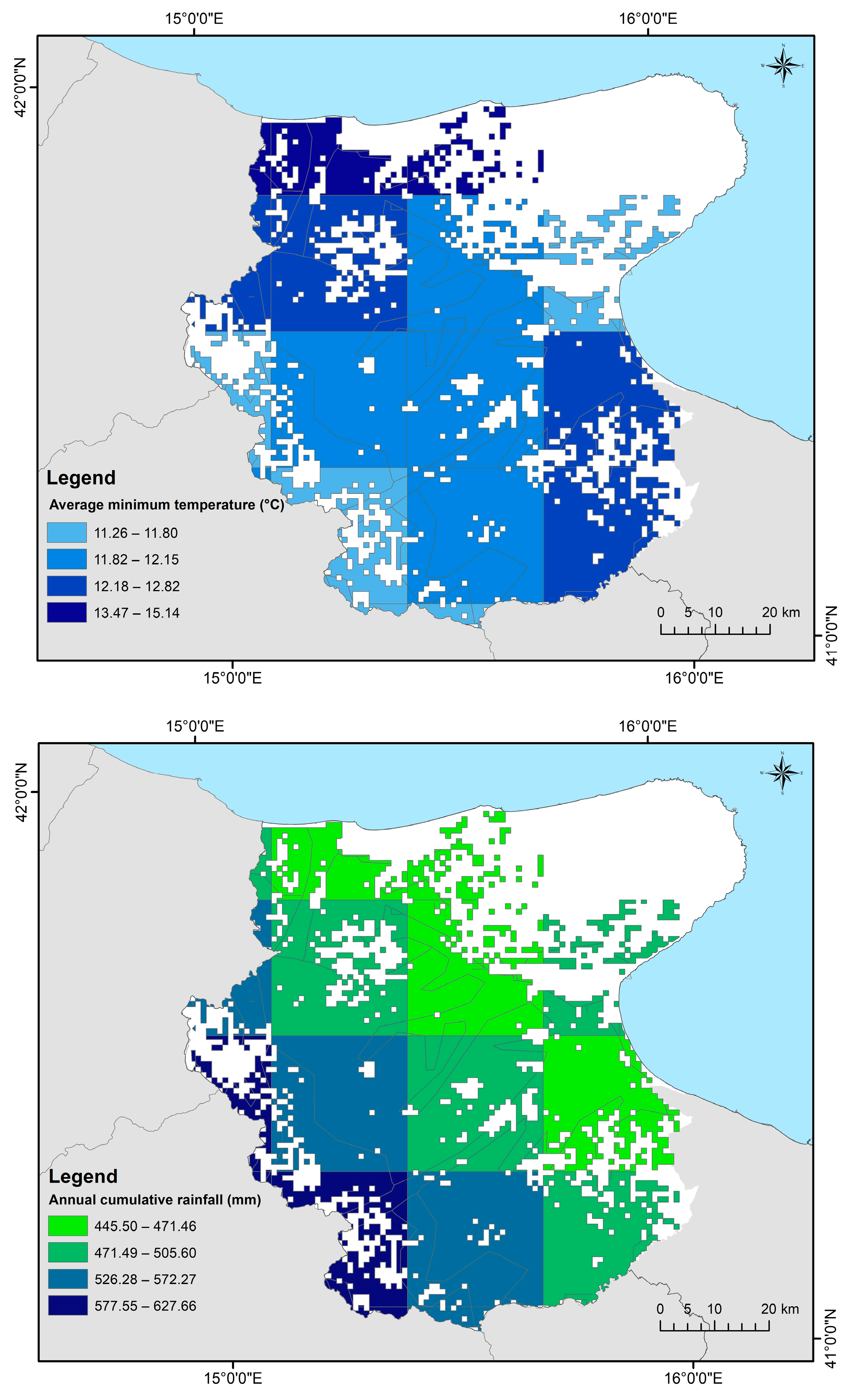
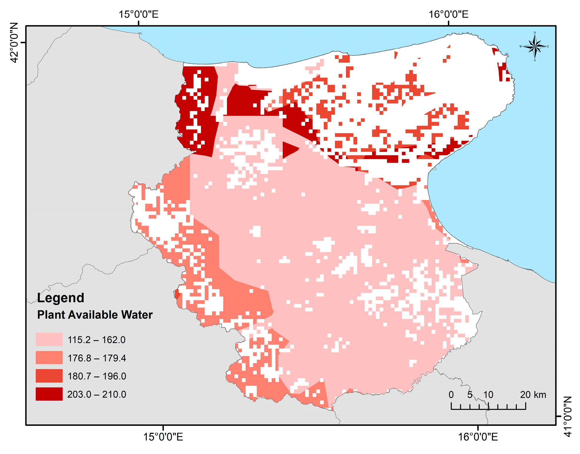
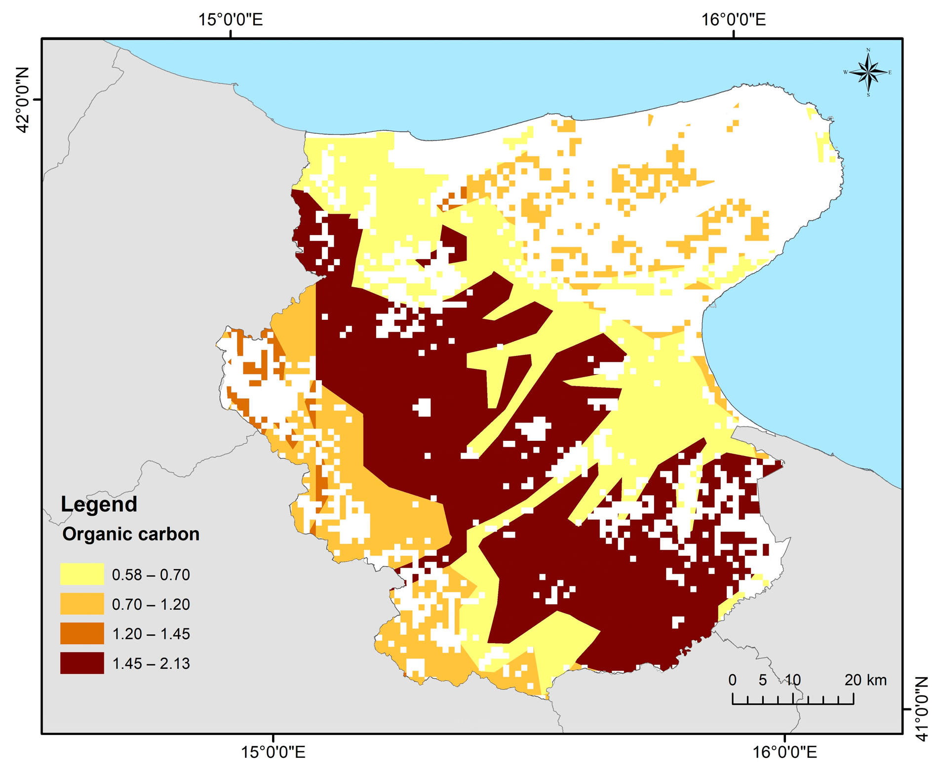
3.1. Pedo-Climatic Characterization of the Area

Regarding the annual thermal data (average annual temperatures for the period 2010–2023), the central (plain) area and part of the northern area experienced the highest maximum temperatures (around 22 °C) compared to the inland hilly areas, with differences ranging from +2 °C to +4 °C (Figure 3). The northern part of the region exhibited the highest minimum temperatures compared to the rest of the analyzed climatic area, with annual averages up to 15 °C, i.e., up to 4 °C higher than the colder areas in the extreme western part (Figure 3).

The annual cumulative rainfall showed clear differences between the different areas of Capitanata. The western area, where durum wheat is cultivated, is characterized by annual rainfall ranging between 530 and 630 mm, which gradually decreases towards the eastern plain (reduction in cumulative rainfall of up to 180 mm per year). The trend in cumulative rainfall follows the topography of the Capitanata plain, gradually increasing from the flat area in the east (around 460 mm per year) to the hilly area in the west (around 600 mm per year; Figure 3).

The differences recorded for this climatic variable reached peaks of about 180 mm, corresponding to an increase of 17% between the rainiest areas in the hilly zone compared to the central zone, up to 33% when the westernmost area is compared to the easternmost one. Plant Available Water (PAW; Figure 4) ranges from a minimum of 15 mm to a maximum of 210 mm. Most of the territory has soils with a plant water availability of 115 to 163 mm, concentrated in the central area of the territory, with higher PAW values bordering the western area (up to 196 mm) and the north of the territory (up to 210 mm). It should be noted that AquaCrop-GIS uses this parameter, in addition to depth, to characterize soils, which is necessary to formalize soil water dynamics. The percentage of soil organic carbon (OC, %; Figure 5) was higher in the central strip of the cultivation area (from north to south), with values ranging from 1.45% to 2.13%. The areas surrounding this central strip were characterized by the lower levels of organic carbon, with percentages ranging from 0.70 to 1.45% in the hilly area to the west, and a minimum of 0.58–0.70% in the easternmost zone of the area.

The initial OC values were fed into the CWFP application to calculate the evolution of soil organic carbon and thus the emissions resulting from the evolution of this parameter.

3.2. Environmental Impact from Soil and Crop Management

The total CO₂_eq emissions associated with wheat cultivation were approximately 1201.3 kg ha⁻¹ (

Table 1. Soil and crop management of durum wheat by activity and associated environmental impacts (CO₂_eq). For baling and residue decomposition, the average (and standard deviation) is reported due to the variable response of the crop under different management and pedo-climatic conditions.

Operation	Passages	Amount	Fertilizer	CO2_eq
	n°	kg ha−1	% N	kg ha−1
Soil management
Plowing	1			121
Disk harrowing	2			161.4
Rotary tilling	1			80.5
Other
Sowing	1			24
Harvest	1			162
Baling of straw	1	7657.9 (±516.7)		74.4 (±5.0)
Fertilizer
Ammonium nitrate	1	100	34	376.4
Urea	1	50	46.6	126.1
Residue decomposition		1351 (±91.2)		75.9 (±9.2)

). It is important to note that the amount of straw baled and removed, as well as the amount of straw left on the soil, varied depending on the management (sowing date and irrigation) and pedo-climatic context (i.e., available plant water, bulk density, and organic carbon). Therefore, unlike the impacts associated with other crop operations, which were fixed (and thus had a single value), the values for baling and decomposing residues were variable, and therefore, mean values and standard deviations were provided. Among these activities, fertilizer application emerged as a major contributor, with ammonium nitrate application alone accounting for a significant proportion at 376.4 kg ha⁻¹ and urea application resulting in emissions of 126.1 kg ha⁻¹. These nitrogen-based fertilizers not only contributed to direct emissions during application, but also facilitated the release of N₂O, a potent greenhouse gas, through processes such as nitrification and denitrification in the soil. Soil management practices had a significant impact on CO₂_eq emissions, with disk harrows, plowing, and rotary tillage together contributing to a significant proportion of total emissions (362.9 kg ha⁻¹). Other operations such as seeding, baling, and harvesting contributed to 260.4 kg ha⁻¹ of CO₂_eq emissions. The subsequent decomposition of straw residues left on the field also contributed to emissions.

However, the emission value associated with the removal of straw residues may not have contributed significantly to CO₂_eq emissions compared to other activities. Looking at the breakdown of emissions as a percentage of total CO₂_eq emissions, ammonium nitrate application accounted for approximately 31.4% of total emissions, while harvesting and disk harrowing each contributed approximately 13.5%. The lowest value in terms of CO₂_eq emissions came from the decomposition of straw residues (6.3%). Finally, other activities, including plowing, sowing, and straw baling, together accounted for about 35.4% of total emissions.

3.3. System Performance

Clear patterns emerge regarding the productivity and environmental impacts associated with different sowing dates and irrigation practices in durum wheat production (

Table 2. Yield and environmental impacts associated with different sowing dates and irrigation practices in durum wheat production. Different letters (a, b, c, d, e) indicate values that are significantly different from each other based on the Tukey HSD test (p < 0.05).

Sowing	Irr	Yield	Water Supply	CO2_eq	CFP	GreenW	BlueW	TW	WFP
		kg ha−1	mm	kg ha−1	kg CO2_eq kg Yield−1	mm	mm	mm	mm Water kg Yield−1
15_oct	no	5432 (471) b		1206 (12.8) ab	0.199 (0.030) c	3901 (339) b	1987 (24.5) de	5887 (327) c	1.086 (0.029) c
01_nov	no	5573 (332) ab		1209 (9.5) ab	0.197 (0.030) c	3999 (239) ab	1999 (14.9) e	5999 (254) c	1.078 (0.019) c
15_nov	no	4983 (429) d		1190 (13.0) c	0.244 (0.042) a	3574 (308) c	1981 (15.8) e	5556 (324) d	1.119 (0.033) b
15_oct	yes	5473 (476) b	13 (4.8) c	1208 (12.9) b	0.197 (0.030) c	3931 (342) b	2114 (60.6) c	6045 (383) bc	1.106 (0.029) b
01_nov	yes	5722 (310) a	28 (9.0) b	1214 (8.6) a	0.186 (0.028) d	4107 (223) a	2280 (95.0) b	6387 (283) a	1.117 (0.020) b
15_nov	yes	5240 (426) c	41 (10.4) a	1199 (12.5) d	0.220 (0.037) b	3760 (306) d	2400 (115.3) a	6160 (397) b	1.178 (0.028) a

). Firstly, in terms of productivity, the early-November sowing date consistently produced the highest average yield under all conditions, with approximately 5573 kg ha⁻¹ without irrigation and 5722 kg ha⁻¹ with irrigation. In contrast, the later sowing dates had lower yields, ranging from about 4983 kg ha⁻¹ (rainfed) to 5240 kg ha⁻¹ (with 41 mm of water supply). This difference in yield between the early-November and mid-November sowing dates represents an average increase of 11.8% without irrigation and 9.2% with irrigation, indicating a clear advantage for the early-November sowing date in terms of grain productivity. The earlier sowing date (15 October) showed the average grain yield with a mean value of 5452 kg ha⁻¹ for both rainfed and irrigated management.

The mid-November sowing date consistently showed higher CO₂_eq emissions per kilogram of grain compared to other dates, with values ranging from approximately 0.220 kg CO₂_eq kg/yield under irrigated management to 0.244 kg CO₂_eq kg/yield under the rainfed option. In particular, CFP emissions associated with the late sowing date were on average 21% higher compared to early-November and 17% higher compared to mid-October. Again, mid-October sowing resulted in CFP values intermediate between the other two sowing options, with emissions just over 3% higher than early-November sowing, but 17% lower than late sowing. GreenW consumption was linked to the productivity of the cropping system, and thus, higher values were obtained for sowing in early November both under rainfed management (+3% compared to 15 October and +11.9% compared to 15 November) and under irrigation (+4.5% compared to 15 October and +9.2% compared to 15 November). There were no significant differences in BlueW between the different sowing dates, except for irrigation, which accounted for 6.4%, 14%, and 21% in the calculation of this parameter when comparing rainfed and irrigated cropping systems for the first, intermediate, and last sowing dates, respectively. As a result, TW along the durum wheat production chain was higher on irrigated plots than on rainfed plots, albeit modestly (+6.5%), indicating that most of this consumption was mainly due to the green component (65%) and within the blue component, and irrigation represented just under 16%. Despite the modest increase in blue water due to water supply, WFP remained comparable between rainfed (1.09 m³ kg⁻¹) and irrigated (1.13 m³ kg⁻¹) regimes, with an increase of 3.6% for the latter.

3.4. Weighting of Key Factors on Productivity and Environmental Performance

The one-way ANOVA was used to determine whether and to what extent the variability in productivity and environmental performance of the cropping system depended on the pedo-climatic context, irrigation management, and sowing date. For this analysis, the sources of variation included the climatic zones, the soils, the three sowing dates, and the use or not of irrigation water. The ANOVA showed that each source of variation, when considered individually, was highly significant in modulating durum wheat productivity, GHG emissions, water use, and finally CFP and WFP (p < 0.001;

Table 3. The one-way analysis of variance (ANOVA) to assess the relationship between sources of variation (pedo-climatic and crop management variables) and cropping system performance and environmental sustainability.

Source	Variable	Sum Square	DF	Mean Square	F	F Crit	p > F
Soil
	Yield	63,984,288	71	901,187	9.85	1.33	<0.001
	CO2_eq	50,632	71	713	7.95	1.33	<0.001
	CFP	0.4131	71	0.0058	9.79	1.33	<0.001
	TW	42,839,751	71	603,377	6.45	1.33	<0.001
	WFP	0.233	71	0.0033	2.24	1.33	<0.001
Irrigation
	Yield	2,395,958	1	2,395,958	10.85	3.86	0.001
	CO2_eq	2566	1	2566	13.73	3.86	<0.001
	CFP	0.017	1	0.017	11.75	3.86	<0.001
	TW	15,892,306	1	15,892,307	112.75	3.86	<0.001
	WFP	0.172	1	0.172	126.16	3.86	<0.001
Sowing time
	Yield	21,206,664	2	10,603,332	60.08	3.02	<0.001
	CO2_eq	21,163	2	10,581	73.50	3.02	<0.001
	CFP	0.132	2	0.066	57.38	3.02	<0.001
	TW	8,401,657	2	4,200,829	26.46	3.02	<0.001
	WFP	0.2521	2	0.1261	106.93	3.02	<0.001
Climate
	Yield	23,607,299	16	1,475,456	8.35	1.67	<0.001
	CO2_eq	19,082	16	1193	7.75	1.67	<0.001
	CFP	0.1051	16	0.0066	5.22	1.67	<0.001
	TW	13,605,671	16	850,354	5.61	1.67	<0.001
	WFP	0.1244	16	0.0078	5.09	1.67	<0.001

).

However, the results obtained did not allow for a comprehensive assessment of the influence of each source of variation relative to the others on the variables analyzed. To rank the influence of climate, soil, sowing date, and irrigation water use globally, the sensitivity analysis (Equation (14)) was carried out to map the effects (Iw) on a scale from 0 (no effect) to 1 (maximum effect). For crop productivity (Figure 6a), sowing date emerged as the factor most responsible for the variability of this parameter (Iw = 0.69), followed by irrigation management (Iw = 0.16), and then by soil and climate. The same trend was observed for GHG emissions (Figure 6b), where the CO₂_eq generated by the cropping system depended largely on the three sowing dates, followed by the use or not of irrigation water, and then the pedo-climatic context. As the CFP is closely linked to yield and CO₂_eq, it was found that, for this parameter too, the sowing date had the greatest impact on the environmental sustainability expressed by this index (Figure 6c). In contrast to the previous observations, for TW, irrigation management had the greatest weight in modulating the water consumption of the cropping system (Iw = 0.74, Figure 7a), followed by the sowing date (Iw = 0.19) and, to a lesser extent, climate and soil. Relating TW to grain produced (Figure 7b) confirmed that this parameter was the most sensitive to irrigation management (Iw = 0.56), with the sowing date (Iw = 0.41) not far behind, while climate and soil remained lower in the ranking.

3.5. Comparative Variability Analysis of Cropping System Response to Primary Drivers

The cumulative probability function of the analyzed variables, based on the sources of variation with the greatest impact (highest Iw values; specifically, irrigation management and sowing date), was used to measure the magnitude of these sources across the different cropping options. For yield (Figure 8), the median (50th percentile) was 5389 kg ha⁻¹ for the rainfed option (NO_IRR) and 5537 kg ha⁻¹ for the irrigated option (IRR). Using the 25th percentile as a critical threshold for significantly low yields, the value was 5071 kg ha⁻¹ for NO_IRR, while it increased to 5277 kg ha⁻¹ for IRR. A similar trend was observed for the 75th percentile, used as a threshold for above-average yields. This was 5775 kg ha⁻¹ for IRR and slightly decreased to 5718 kg ha⁻¹ for rainfed option. Overall, the main effect of irrigation at flowering was to reduce inter-annual variability compared to rainfed management. Specifically, comparing the differences in yield at the 25th and 75th percentiles relative to the mean, the difference at the lower threshold was −258 kg ha⁻¹ for NO_IRR (−4.8%) and −211 kg ha⁻¹ for IRR (−3.8%). For the upper threshold, the differences were +388 kg ha⁻¹ for NO_IRR (+7.3%) and +297 kg ha⁻¹ for IRR (+5.4%).

In terms of CO₂_eq, no significant differences were observed between the two irrigation management practices. The cumulative distribution data clustered around the median value of 1208 kg ha⁻¹. The percentage variations relative to the mean value of GHG emissions were around +1% for the 75th percentile and −0.6% for the 25th percentile (Figure 8). In contrast, the analysis of the CFP showed that this sustainability index remained stable when considering both NO_IRR and IRR (Figure 8). The median value for NO_IRR was slightly less than 4% higher than for IRR. The deviations of the cumulative probability function values at the 25th and 75th percentiles were also aligned between the two irrigation management practices. However, the deviation of the values calculated at the two thresholds of the cumulative probability function (relative to the mean CFP value), although similar for both irrigation practices, ranged from approximately +12% for the 75th percentile to −13% for the 25th percentile. These results showed that, on the one hand, CFP could generally be considered a sufficiently stable indicator of environmental sustainability, independent of irrigation management, but that its variability around the mean was closely linked to the variability of grain yield (considering that the numerator, CO₂_eq, remained within a narrow range of values, as previously reported). For TW (Figure 9), the median value of IRR was higher compared to NO_IRR (6291 m³ ha⁻¹ vs. 5863 m³ ha⁻¹). The variability of the values, expressed by the deviation of the 25th and 75th percentiles from the mean, remained limited to a few percentage points, but shifted towards higher values for IRR compared to NO_IRR. The differences observed between the values of the two irrigation regimes were mainly due to the water evapotranspired by the crop (with blue water depending on the same crop management and reduced irrigation volumes), which, in turn, was linked to the biomass accumulation of the durum crop. This was reflected in the WFP, whose median value was slightly higher for IRR than for NO_IRR (Figure 9). Ultimately, WFP proved to be sufficiently stable both between the two irrigation regimes and within each irrigation regime.

When analyzing the cumulative probability functions of the production performance of the durum wheat cropping system as a function of the sowing date (averaging the irrigation management data; Figure 10), it was observed that sowing in mid-November produced a mean yield (5195 kg ha⁻¹) lower than sowing on 15 October (5585 kg ha⁻¹) and especially in early November (5718 kg ha⁻¹). In addition, not only were the yield data at the 25th and 75th percentiles lower at the latest sowing date than at the other two dates, but the deviations at these two critical thresholds (−6.25% at the 25th percentile and +6.05% at the 75th percentile) relative to the mean were greater than at the other two sowing dates (values ranging from −3.82% to +5.74%). In contrast to grain yield, CO₂_eq was similar for the three sowing dates, with median values ranging from 1197 kg ha⁻¹ for mid-November sowing to 1213 kg ha⁻¹ for early-November sowing (Figure 10). As GHG emissions are largely influenced by crop management practices (such as conventional tillage), the resulting values at the 25th and 75th percentiles were negligible, with increases (75th percentile) and decreases (25th percentile) of less than one percentage point. In any case, the estimation of the CFP, especially in relation to the crop yield, varied according to the sowing period, determining different sustainability indices for this parameter (Figure 10).

Indeed, the median value was the lowest for sowing on 1 November (0.193 kg m³ kg⁻¹), followed by sowing in mid-October (0.205 kg kg⁻¹) and finally sowing in mid-November (0.258 kg kg⁻¹). However, in all three sowing periods, the variability of intra-annual CFP values increased compared to yield and CO₂_eq. At the 25th percentile, CFP was 0.168 kg kg⁻¹ for both the 15 October and 1 November sowings, although the percentage deviation was −15.5% for the former and −11.84% for the latter. Higher was the value recorded at the 25th percentile of the cumulative probability function for the mid-November sowing, where the CFP was 0.201 kg kg⁻¹ (−13.37% relative to the mean). This period also showed worse (higher) values for this sustainability index at the 75th percentile (0.258 kg kg⁻¹) compared to sowing on 1 November (0.217 kg kg⁻¹) and mid-October (0.222 kg kg⁻¹), with percentage deviations ranging from +11.50% to +13% relative to the mean.

Sowing in mid-November proved to be the least environmentally friendly for WFP (Figure 11), as this sowing date consistently maintained higher WFP values throughout the cumulative probability function curve from the 25th to the 75th percentile (albeit with variations limited to around 5%). As for the CFP, this index also remained within moderate variations considering the two thresholds (25th and 75th percentile) of the cumulative probability curve (Figure 11), with the largest deviations from the mean occurring for the mid-November sowing (−3.21% to +2.58%) and the smallest for the early-November sowing (−1.72% to +1.81%). For TW, the trends of the cumulative probability function curves followed their respective yields, with higher productivity correlating with increased water use. Specifically, the median values were 6208 m³ ha⁻¹, 6052 m³ ha⁻¹, and 5804 m³ ha⁻¹ for 1 November, 15 October, and 15 November, respectively. Sowing in the two November dates also ensured lower inter-annual variability for TW compared to the mean, with percentage differences ranging from +4.21% at the 75th percentile to −3.69% at the 25th percentile (mean for both dates), compared to +7.42% (75th percentile) and −5.55% (25th percentile) for October sowing.

4. Discussion

In this study, the productive and environmental performance of durum wheat was evaluated in response to 216 combinations of different crop management practices (sowing dates and irrigation), various soil types, and differing climatic conditions (ranging from flat to hilly areas, and from inland to coastal zones, typical of the territory examined for this modeling exercise). This was carried out using a version of AquaCrop that also integrates the spatialization of data related to the cropping system. The simulation algorithms of AquaCrop-GIS are the same as those underlying the functionality of AquaCrop at the point scale [55]. The model’s simulation output is based on the crop phenotype, which is determined by the interaction between the plant’s genetic traits and pedo-climatic variables. This interaction reaches its peak in the calibration of the parameters and coefficients used in the crop-specific simulation algorithms, in this study, for winter durum wheat cultivated in the Capitanata area [62].

Pedo-climatic variables play a fundamental role in modulating the morpho-productive response of durum wheat within AquaCrop, as they determine the dynamics of canopy expansion and phenological phases (temperature), the crop’s potential evapotranspiration (from ET0), thermal stress (from temperatures outside the optimal range), and water stress (from soil-specific characteristics, such as depth, water availability for plants, and rainfall). The same applies to crop management practices, such as sowing and irrigation dates (as reported in this study), which, in combination with different pedo-climatic scenarios, lead to diverse responses from the cropping system. The combination of all these pedo-climatic variables and management practices, if applied in AquaCrop’s point-scale version, would have required the preparation of numerous input files (such as climate, soil, and management) to generate individual output scenarios, which would then be integrated into a spreadsheet for subsequent processing. In contrast, the AquaCrop-GIS version allowed the creation of just a few input files (spreadsheets that gather all information related to management, crop parameters, and pedo-climatic conditions in their various combinations), the processing of which produced a single output sheet, enabling rapid, precise, and easily interpretable analysis. Therefore, the application of AquaCrop-GIS allowed for the exploration of the durum wheat cultivation system over an area of approximately 7000 km², diverse in terms of climatic patterns and soil characteristics. This is of fundamental importance, as the insights derived from this modeling exercise did not concern only a few pedo-climatic points but rather represented a large area, providing values that are highly representative of the region, as shown in Table 2. The extensive data were processed not only to obtain means and standard deviations of the analyzed variables but also to offer specific guidance on aspects related to crop management (specifically sowing and irrigation dates), in terms of which of these management practices are suitable for optimizing various aspects of the cropping system.

Firstly, the simulation scenarios provided important insights into the effects of sowing dates and irrigation practices on durum wheat productivity.

Three sowing dates (15 October, 1 November, and 15 November) and two irrigation scenarios (rainfall and additional irrigation during flowering (up to 60 mm of total irrigation water)) were investigated. The results highlighted the significant influence of sowing date on yield. Sowing in early November typically yielded better results than later sowing dates, due to better adaptation to favorable climatic conditions during the critical growth stages of the crop, as indicated by the longer growing cycle (177 days) compared to the other two sowing dates (with an average of 173 days). This confirms what has been reported by other authors [71], who have shown how sowing durum wheat in Mediterranean environments within 30-day time windows resulted in yield variations ranging from 5% (in the Apulia region, Southern Italy) to 56% (in the province of Settat, Morocco). However, a study based on empirical models demonstrated that the optimal sowing date to maximize winter wheat production was from October 1 to October 15 [72]. On the other hand, a literature review reported that, in winter-sown durum wheat, early sowing when temperatures are above the optimum produces poor plants and even a higher seeding rate cannot compensate for a low yield. Moreover, under late-sown conditions, wheat faces low temperatures in the earlier stages and high temperatures in the later stages of the growing season, which, due to a lack of favorable moisture for better growth and development at this stage, causes yield reduction [73].

Combining information from AquaCrop-GIS, it emerged that GDD at physiological maturity were almost identical across the three sowing dates (between 2424 °C and 2428 °C), but spread over a longer crop cycle in the early-November sowing, indicating that this cropping system experienced lower temperatures compared to the other two sowing dates (on average 13.6 °C versus 14 °C), resulting in reduced thermal stress responsible for the shortening of the crop growing cycle. Additionally, the crop evapotranspiration (ETc) was 315 mm (averaging values of NO_IRR and IRR), an intermediate value between 288 mm for the October sowing and 323 mm for the mid-November sowing. The water evaporated from the soil, thus not used productively by the crop, was on average 113 mm in 15_10 and 15_11, higher than 109 mm in the early-November sowing. However, the water use efficiency for the water consumed in 15_11 (15.8 kg yield mm ETc⁻¹) was lower compared to 01_11 (17.98 kg yield mm ETc⁻¹) and 15_10 (18.9 kg yield mm ETc⁻¹). In the case of 15_10, although the water use efficiency was higher compared to that in early-November sowing, the shorter crop cycle (due to less favorable thermal conditions) led to a lower productivity performance compared to 01_11, but higher than that in the late-November sowing.

The use of supplemental irrigation during flowering was found to be beneficial in stabilizing yields rather than improving crop performance, in line with the modest productivity gains found by other authors when durum wheat was irrigated during flowering [74]. Although other authors demonstrated that irrigation during flowering significantly increased the productive performance of wheat, it was not accompanied by a higher efficiency of water use [75].

In the modeling exercise reported in this paper, the data processing demonstrated how this practice mitigated the adverse effects of water stress during a critical developmental phase (flowering stage), thereby increasing yield stability over the years rather than providing significant increases in grain yield. This was evidenced by the higher yield when comparing grains obtained at the low threshold percentile of the cumulative probability density function. For example, at the 25th percentile, the yield value for NO_IRR was 5034 kg ha⁻¹, while in the irrigated scenario, this value was found at the 15th percentile, indicating a lower probability (by 10 percentage points) of obtaining such a low yield.

Concerning the environmental aspect, the fertilizers (type and amount) specified for this cropping system (ammonium nitrate and urea under conventional tillage) were the main source of GHG emissions (both direct and indirect), contributing about 48% of the total environmental impact. The significant contribution of nitrogen-based fertilizers to the release of CO₂_eq into the atmosphere found in our study aligns with other investigations, which emphasized the critical role of efficient nitrogen management in reducing greenhouse gas (GHG) emissions in the Mediterranean wheat systems [3]. Therefore, this agro-input is confirmed as one of the main hotspots regarding the environmental sustainability of durum wheat cultivation under conventional tillage, as identified by other authors in studies on durum wheat grown in the Apulia region [76].

Soil management, particularly seedbed preparation operations, was the second most emission-intensive process, followed by other operations related to sowing, harvesting, and packing. The choice of tillage practice was reported to be a major option for significantly reducing greenhouse gas emissions, with reductions of up to 42% when switching from conventional tillage to no-tillage [77]. In addition, leaving straw on the soil can result in a CO₂_eq saving of around 6% (due to reduced straw collection and baling). However, the transition from conventional tillage to alternative tillage methods (such as minimum tillage and no-tillage) may, at least in the short-to-medium term, involve trade-offs that offset the reduction in GHG emissions and/or performance in terms of CFP.

Indeed, reduced or even no-tillage has been reported to reduce cereal productivity [78,79,80], with losses of up to −10% for minimum tillage and −20% for no-tillage. The other issue associated with soil management alternatives to conventional tillage is the increased use of pesticides for weed control. In fact, reducing tillage and/or leaving straw on the soil creates an optimal environment for weed development (seeds remain on the surface but are “protected” by crop residues). The residues also reduce the effectiveness of pesticides [81]. This may result in the introduction of herbicides where they were not previously used, or increased rates where they were. The use of herbicides in herbaceous cropping systems contributes a significant share of GHG emissions, both for production and application (302 kg CO₂_eq ha⁻¹) [82] and for indirect GHG emissions (up to 383 kg CO₂_eq ha⁻¹) [83]. Recent studies highlighted the significant impact of tillage practices on soil health and GHG emissions. The disruption of soil’s physical structure due to tillage altered the soil environment and fertility, affecting microbial decomposition and root respiration, which in turn influenced GHG emissions [84]. While the effects of tillage on crop yield remained uncertain, no-tillage practices were associated with increased emissions of CO₂, CH₄, and N₂O. Specifically, no-tillage was found to increase CO₂ emissions by 7.1%, CH₄ emissions by 20.8%, and N₂O emissions by 12.0% [85].

Conversely, reduced-tillage techniques offered advantages by improving soil aeration and reducing moisture, potentially leading to higher soil organic matter and lower N₂O emissions. These practices were considered beneficial for carbon storage and overall economic outcomes [86]. On the other hand, it has been demonstrated that, while deep tillage exacerbated CO₂ emissions, it did not similarly influence the emissions of other potent greenhouse gasses like N₂O and CH₄ [87].

In any case, the analysis carried out in this modeling exercise showed that, even with the same management practices (conventional tillage, which represents almost the entire agronomic practice of durum wheat cultivation in monoculture), it was possible to reduce the environmental impact of the cropping system (i.e., CFP). This reduction was achieved by modifying two practices: sowing date and irrigation. These adjustments do not require significant changes in agricultural practices, machinery, or equipment. This was made possible by the increase in crop productivity, which is the denominator in the calculation of CFP. The potential to mitigate the environmental impact of the durum wheat cropping system by reducing CFP indicator was also demonstrated by other studies, which showed that the choice of appropriate agronomic practices, including the optimal seeding date, could improve crop productivity without increasing production inputs [88,89]. Indeed, this index was lower in the cropping system with higher yields (i.e., sowing in early November, with or without irrigation), while the highest values (indicating less environmentally friendly cropping systems) were observed with later sowing, with or without water supply. The high variability of this index value has also been reported in several other studies, confirming that productivity is the key factor in modulating CFP [90,91,92], with the highest values observed in systems with the lowest productivity [93].

An interesting observation was made when analyzing the cumulative distribution function. In late sowing, the risk of obtaining high CFP values (expressed as 0.258 kg CO₂_eq per kg yield at the 75th percentile), compared to the average, was only observed for sowing in mid-November and not for sowing in mid-October or early-November. These two sowing dates never produced CFP values equal to or greater than this magnitude, indicating that they are clearly preferable for reducing the environmental impact associated with this index. Irrigation management also proved to be important in reducing the CFP value. Indeed, when analyzing the cumulative probability density curves, IRR shifted the curve to the left compared to NO_IRR, highlighting how this practice, although based on small amounts of water supply during the flowering stage, could promote more stable yields, less susceptible to the climatic vagaries of the growing season, and ultimately reduce CFP. Although irrigation plays a key role in reducing CFP, in the cropping systems analyzed, its impact on the water consumption of the system was limited. In fact, the impact of the irrigation volumes formalized in this research was negligible, amounting to a maximum of 1.7% (in the system with the highest irrigation water supply) in terms of BlueW. However, it promoted more stable yields and facilitated better use of water resources. This explains why, in the most productive management scenarios (with irrigation and sowing in early November), TW was higher, due to increased GreenW consumption rather than an increase in BlueW. This trend is also confirmed by other authors, where modest increases in irrigation water led to increases in GreenW consumption [94]. However, the trend in WFP showed an inverse relationship with CFP.

While an increase in productivity justified a reduction in the latter index (under similar crop and soil management conditions), WFP noted a lack of proportionality between increased water use and grain yield. Instead, this sustainability index was negatively affected by increased productivity. In other words, under rainfed conditions, the crop used rainwater more effectively, so that lower (though not dramatic) yields corresponded to better sustainability in terms of WFP. This is consistent with findings from previous research, where better water use efficiency in cereals under conditions of reduced water supply has been widely observed compared to better water supply conditions [95,96,97]. Similarly, it was found that the irrigation of durum wheat, although it resulted in nearly doubled yields compared to non-irrigated crops (5.4 t ha⁻¹ vs. 2.8 t ha⁻¹), did not correspond to an equal improvement in WFP. In fact, rainfed plants were able to reduce the value of this index by 14% compared to those receiving supplemental water (1.05 m³ kg yield⁻¹ vs. 1.22 kg yield⁻¹) [98]. The results obtained and discussed here reveal a nuanced trade-off between reducing CFP and increasing WFP in durum wheat production. While minimizing CFP is crucial for mitigating environmental impacts, optimizing WFP is equally important for ensuring efficient water use, especially in view of its increasing scarcity. The reduction in GHG emissions is closely linked to the reduction in agro-technical inputs. Switching from conventional tillage to alternative soil management practices (such as minimum tillage and no-tillage) could have a positive impact on the environmental sustainability of a cropping system (such as durum wheat). However, this would require the replacement of machinery, which is a major challenge for most durum wheat farms in the study area and is unlikely to be achievable in the short term. Mineral nitrogen fertilization is another factor to be considered, and here, a reduction in dose and/or the use of alternative forms of fertilization (such as compost) could be beneficial.

Such changes need to be carefully evaluated in terms of potential productivity loss; as the aim is to optimize WFP, this study has shown the importance of maintaining adequate yields to avoid reducing CFP values. In addition, leaving straw on the soil rather than removing it can improve the environmental sustainability of the cropping system by increasing soil organic carbon stocks. However, it is important to consider the trade-offs associated with increased N₂O and methane emissions due to straw decomposition [99]. Finally, the use of the WFP to assess the environmental sustainability of durum wheat production, at least under the pedo-climatic conditions and irrigation levels used here, can be tricky and requires careful evaluation. A reduction in this index inevitably involves a reduction in GreenW, which represents the majority of the water used, even taking into account the modest amounts of irrigation water used here (which have a minimal impact on BlueW). The results show that reducing GreenW is associated with lower yields (less evapotranspired water) but giving instructions in this direction (produce less to reduce water consumption and increase WFP) is not sustainable from other perspectives (such as economic returns). In this case, instead of trying to minimize this index separately from CFP, it is advisable to optimize both indices, including by choosing specific sowing dates (e.g., early November) combined with modest irrigation volumes during the flowering period (around 300 m³ ha⁻¹).

5. Conclusions

This study introduces an innovative approach by integrating the AquaCrop-GIS model with the Carbon and Water Footprint (CWFP) tool to evaluate both productivity and environmental sustainability in durum wheat production. The novelty of this research lies in using these tools together to assess the trade-offs between yield optimization and environmental impacts, such GHG emissions and water use, across different sowing dates and irrigation regimes. Unlike traditional studies that assess either agronomic performance or environmental impacts in isolation, this research provides a comprehensive framework linking crop management practices to sustainability outcomes.

The modeling analysis of durum wheat cropping system revealed the significant influence of sowing dates and irrigation practices on both productivity and environmental sustainability. Three different sowing dates and both rainfed and irrigated scenarios were examined to assess their effects on grain yield, GHG emissions, and water use. In terms of productivity, early-November sowing outperformed other dates, with higher average grain yields under all water regimes and pedo-climatic conditions. Supplemental irrigation during flowering was found to be particularly beneficial in stabilizing yields and mitigating water stress during critical growth stages.

From an environmental standpoint, nitrogen-based fertilizers emerged as a major contributor to GHG emissions, with soil management practices also significantly impacting emissions. The analysis showed that sowing date and irrigation management played key roles in modulating the CFP and WFP. Sowing in early November, combined with supplemental irrigation, led to lower CFP values, indicating greater environmental sustainability compared to later sowing dates. However, the increased productivity resulting from optimized management practices also led to higher WFP values, underscoring the delicate balance between productivity and water conservation, especially for GreenW component.

In terms of sustainability, the results suggest that, while it may not be possible to maximize both environmental sustainability indices simultaneously, the optimization of both can be achieved through the careful management of sowing dates and deficit irrigation. This is particularly factual where significant changes to the cropping system, such as reduced tillage, changes in fertilizer management, and variations in straw management, not only require investment of time, technology, and equipment but also require the consideration of how these changes may affect other variables such as productivity, increased chemical use, and increased GHG emissions.

This dual focus on productivity and environmental sustainability, coupled with the innovative application of modeling tools, offers actionable insights for improving durum wheat production systems, particularly in Mediterranean environments.

References

1. Falcone, G.; Stillitano, T.; Montemurro, F.; De Luca, A.I.; Gulisano, G.; Strano, A. Environmental and Economic Assessment of Sustainability in Mediterranean Wheat Production. Agron. Res. 2019, 17, 60–79. [Google Scholar] [CrossRef]
2. FAO. FAO Statistical Yearbook 2013—World Food and Agriculture; FAO Statistical Yearbook; FAO: Rome, Italy, 2012; ISBN 978-92-5-107396-4. [Google Scholar]
3. Tedone, L.; Ali, S.A.; Mastro, G.D. Optimization of Nitrogen in Durum Wheat in the Mediterranean Climate: The Agronomical Aspect and Greenhouse Gas (GHG) Emissions. In Nitrogen in Agriculture—Updates; Amanullah, K., Fahad, S., Eds.; InTech: London, UK, 2018; ISBN 978-953-51-3768-9. [Google Scholar]
4. Martínez-Moreno, F.; Solís, I.; Noguero, D.; Blanco, A.; Özberk, İ.; Nsarellah, N.; Elias, E.; Mylonas, I.; Soriano, J.M. Durum Wheat in the Mediterranean Rim: Historical Evolution and Genetic Resources. Genet. Resour. Crop Evol. 2020, 67, 1415–1436. [Google Scholar] [CrossRef]
5. Ahmad, W.; Ullah, N.; Xu, L.; El Sabagh, A. Editorial: Global Food and Nutrition Security Under Changing Climates. Front. Agron. 2022, 3, 799878. [Google Scholar] [CrossRef]
6. Toscano, P.; Genesio, L.; Crisci, A.; Vaccari, F.P.; Ferrari, E.; Cava, P.L.; Porter, J.R.; Gioli, B. Empirical Modelling of Regional and National Durum Wheat Quality. Agric. For. Meteorol. 2015, 204, 67–78. [Google Scholar] [CrossRef]
7. ISTAT. Available online: https://www.istat.it/it/files//2021/05/Tavole_dati_Indicatori_agro_ambientali_AEIs_2010_19_20_05_2021.xlsx. (accessed on 1 April 2024).
8. Rezzouk, F.Z.; Gracia-Romero, A.; Kefauver, S.C.; Nieto-Taladriz, M.T.; Serret, M.D.; Araus, J.L. Durum Wheat Ideotypes in Mediterranean Environments Differing in Water and Temperature Conditions. Agric. Water Manag. 2022, 259, 107257. [Google Scholar] [CrossRef]
9. Xynias, I.N.; Mylonas, I.; Korpetis, E.G.; Ninou, E.; Tsaballa, A.; Avdikos, I.D.; Mavromatis, A.G. Durum Wheat Breeding in the Mediterranean Region: Current Status and Future Prospects. Agronomy 2020, 10, 432. [Google Scholar] [CrossRef]
10. Todorović, M.; Mehmeti, A.; Cantore, V. Impact of Different Water and Nitrogen Inputs on the Eco-Efficiency of Durum Wheat Cultivation in Mediterranean Environments. J. Clean. Prod. 2018, 183, 1276–1288. [Google Scholar] [CrossRef]
11. Soto-Gómez, D.; Pérez-Rodríguez, P. Sustainable Agriculture through Perennial Grains: Wheat, Rice, Maize, and Other Species. A. Review. Agric. Ecosyst. Environ. 2022, 325, 107747. [Google Scholar] [CrossRef]
12. Ross-Ibarra, J.; Morrell, P.L.; Gaut, B.S. Plant Domestication, a Unique Opportunity to Identify the Genetic Basis of Adaptation. Proc. Natl. Acad. Sci. USA 2007, 104, 8641–8648. [Google Scholar] [CrossRef]
13. Howells, M.; Hermann, S.; Welsch, M.; Bazilian, M.; Segerström, R.; Alfstad, T.; Gielen, D.; Rogner, H.; Fischer, G.; Van Velthuizen, H.; et al. Integrated Analysis of Climate Change, Land-Use, Energy and Water Strategies. Nat. Clim. Change 2013, 3, 621–626. [Google Scholar] [CrossRef]
14. Turral, H.; Burke, J.J.; Faurès, J.-M. Climate Change, Water and Food Security; FAO Water Reports; Food and Agriculture Organization of the United Nations: Rome, Italy, 2011; ISBN 978-92-5-106795-6. [Google Scholar]
15. Cox, T.S.; Glover, J.D.; Van Tassel, D.L.; Cox, C.M.; DeHaan, L.R. Prospects for Developing Perennial Grain Crops. BioScience 2006, 56, 649. [Google Scholar] [CrossRef]
16. Pimentel, D.; Cerasale, D.; Stanley, R.C.; Perlman, R.; Newman, E.M.; Brent, L.C.; Mullan, A.; Chang, D.T.-I. Annual vs. Perennial Grain Production. Agric. Ecosyst. Environ. 2012, 161, 1–9. [Google Scholar] [CrossRef]
17. Gallucci, T.; Lagioia, G.; Piccinno, P.; Lacalamita, A.; Pontrandolfo, A.; Paiano, A. Environmental Performance Scenarios in the Production of Hollow Glass Containers for Food Packaging: An LCA Approach. Int. J. Life Cycle Assess 2021, 26, 785–798. [Google Scholar] [CrossRef]
18. Garcia-Garcia, G.; Azanedo, L.; Rahimifard, S. Embedding Sustainability Analysis in New Food Product Development. Trends Food Sci. Technol. 2021, 108, 236–244. [Google Scholar] [CrossRef]
19. Hatt, S.; Artru, S.; Brédart, D.; Lassois, L.; Francis, F.; Haubruge, É.; Garré, S.; Stassart, P.M.; Dufrêne, M.; Monty, A.; et al. Towards sustainable food systems: The concept of agroecology and how it questions current research practices. A review. Biotechnol. Agron. Soc. Environ. 2016, 20, 215–224. [Google Scholar] [CrossRef]
20. Mäkinen, H.; Kaseva, J.; Trnka, M.; Balek, J.; Kersebaum, K.C.; Nendel, C.; Gobin, A.; Olesen, J.E.; Bindi, M.; Ferrise, R.; et al. Sensitivity of European Wheat to Extreme Weather. Field Crops Res. 2018, 222, 209–217. [Google Scholar] [CrossRef]
21. Trnka, M.; Olesen, J.E.; Kersebaum, K.C.; Skjelvåg, A.O.; Eitzinger, J.; Seguin, B.; Peltonen-Sainio, P.; Rötter, R.; Iglesias, A.; Orlandini, S.; et al. Agroclimatic Conditions in Europe under Climate Change: Agroclimatic Conditions in Europe under CC. Glob. Change Biol. 2011, 17, 2298–2318. [Google Scholar] [CrossRef]
22. Chen, D.; Suter, H.; Islam, A.; Edis, R.; Freney, J.R.; Walker, C.N. Prospects of Improving Efficiency of Fertiliser Nitrogen in Australian Agriculture: A Review of Enhanced Efficiency Fertilisers. Soil Res. 2008, 46, 289. [Google Scholar] [CrossRef]
23. Tomaz, A. An Overview on the Use of Enhanced Efficiency Nitrogen Fertilizers in Irrigated Mediterranean Agriculture. Biomed. J. Sci. Tech. Res. 2017, 1, 1938–1940. [Google Scholar] [CrossRef]
24. Oliveira, P.; Patanita, M.; Dôres, J.; Boteta, L.; Palma, J.F.; Patanita, M.I.; Guerreiro, I.; Penacho, J.; Costa, M.N.; Rosa, E.; et al. Combined Effects of Irrigation Management and Nitrogen Fertilization on Soft Wheat Productive Responses under Mediterranean Conditions. E3S Web Conf. 2019, 86, 00019. [Google Scholar] [CrossRef]
25. Patanita, M.; Tomaz, A.; Ramos, T.; Oliveira, P.; Boteta, L.; Dôres, J. Water Regime and Nitrogen Management to Cope with Wheat Yield Variability under the Mediterranean Conditions of Southern Portugal. Plants 2019, 8, 429. [Google Scholar] [CrossRef] [PubMed]
26. Ali Fallahi, H.; Nasseri, A.; Siadat, A. Wheat Yield Components Are Positively Influenced by Nitrogen Application under Moisture Deficit Environments. Int. J. Agric. Biol. 2008, 10, 6. [Google Scholar]
27. Zeleke, K.T.; Nendel, C. Analysis of Options for Increasing Wheat (Triticum aestivum L.) Yield in South-Eastern Australia: The Role of Irrigation, Cultivar Choice and Time of Sowing. Agric. Water Manag. 2016, 166, 139–148. [Google Scholar] [CrossRef]
28. Liu, W.; Wang, J.; Wang, C.; Ma, G.; Wei, Q.; Lu, H.; Xie, Y.; Ma, D.; Kang, G. Root Growth, Water and Nitrogen Use Efficiencies in Winter Wheat Under Different Irrigation and Nitrogen Regimes in North China Plain. Front. Plant Sci. 2018, 9, 1798. [Google Scholar] [CrossRef]
29. Howell, T.A. Enhancing Water Use Efficiency in Irrigated Agriculture. Agron. J. 2001, 93, 281–289. [Google Scholar] [CrossRef]
30. Katerji, N.; Mastrorilli, M.; Rana, G. Water Use Efficiency of Crops Cultivated in the Mediterranean Region: Review and Analysis. Eur. J. Agron. 2008, 28, 493–507. [Google Scholar] [CrossRef]
31. Zwart, S.J.; Bastiaanssen, W.G.M.; De Fraiture, C.; Molden, D.J. A Global Benchmark Map of Water Productivity for Rainfed and Irrigated Wheat. Agric. Water Manag. 2010, 97, 1617–1627. [Google Scholar] [CrossRef]
32. Pereira, L.S.; Cordery, I.; Iacovides, I. Improved Indicators of Water Use Performance and Productivity for Sustainable Water Conservation and Saving. Agric. Water Manag. 2012, 108, 39–51. [Google Scholar] [CrossRef]
33. Zhang, W.; Liu, G.; Sun, J.; Fornara, D.; Zhang, L.; Zhang, F.; Li, L. Temporal Dynamics of Nutrient Uptake by Neighbouring Plant Species: Evidence from Intercropping. Funct. Ecol. 2017, 31, 469–479. [Google Scholar] [CrossRef]
34. Levidow, L.; Zaccaria, D.; Maia, R.; Vivas, E.; Todorovic, M.; Scardigno, A. Improving Water-Efficient Irrigation: Prospects and Difficulties of Innovative Practices. Agric. Water Manag. 2014, 146, 84–94. [Google Scholar] [CrossRef]
35. Fernández, J.E.; Alcon, F.; Diaz-Espejo, A.; Hernandez-Santana, V.; Cuevas, M.V. Water Use Indicators and Economic Analysis for On-Farm Irrigation Decision: A Case Study of a Super High Density Olive Tree Orchard. Agric. Water Manag. 2020, 237, 106074. [Google Scholar] [CrossRef]
36. Hoekstra, A.Y. Virtual Water Trade: Proceedings of the International Expert Meeting on Virtual Water Trade. 2003, p. 93. Available online: https://ihedelftrepository.contentdm.oclc.org/digital/collection/p21063coll3/id/10351 (accessed on 1 July 2024).
37. Mekonnen, M.M.; Hoekstra, A.Y. The Green, Blue and Grey Water Footprint of Crops and Derived Crop Products. Hydrol. Earth Syst. Sci. 2011, 15, 1577–1600. [Google Scholar] [CrossRef]
38. Ababaei, B.; Etedali, H.R. Estimation of Water Footprint Components of Iran’s Wheat Production: Comparison of Global and National Scale Estimates. Environ. Process. 2014, 1, 193–205. [Google Scholar] [CrossRef]
39. ISO 14046:2014; Environmental Management–Water Footprint–Principles, Requirements and Guidelines. International Organization for Standardization: Geneva, Switzerland, 2014.
40. Steen-Olsen, K.; Weinzettel, J.; Cranston, G.; Ercin, A.E.; Hertwich, E.G. Carbon, Land, and Water Footprint Accounts for the European Union: Consumption, Production, and Displacements through International Trade. Environ. Sci. Technol. 2012, 46, 10883–10891. [Google Scholar] [CrossRef] [PubMed]
41. Rodriguez, C.I.; Ruiz De Galarreta, V.A.; Kruse, E.E. Analysis of Water Footprint of Potato Production in the Pampean Region of Argentina. J. Clean. Prod. 2015, 90, 91–96. [Google Scholar] [CrossRef]
42. Perry, C. Water Footprints: Path to Enlightenment, or False Trail? Agric. Water Manag. 2014, 134, 119–125. [Google Scholar] [CrossRef]
43. Khan, S.; Hanjra, M.A. Footprints of Water and Energy Inputs in Food Production–Global Perspectives. Food Policy 2009, 34, 130–140. [Google Scholar] [CrossRef]
44. Ruddiman, W.F. The Anthropogenic Greenhouse Era Began Thousands of Years Ago. Clim. Change 2003, 61, 261–293. [Google Scholar] [CrossRef]
45. Janzen, H.H.; Beauchemin, K.A.; Bruinsma, Y.; Campbell, C.A.; Desjardins, R.L.; Ellert, B.H.; Smith, E.G. The Fate of Nitrogen in Agroecosystem: An Illustration Using Canadian Estimates. Nutr. Cycl. Agroecosyst. 2003, 67, 85–102. [Google Scholar] [CrossRef]
46. Pattara, C.; Raggi, A.; Cichelli, A. Life Cycle Assessment and Carbon Footprint in the Wine Supply-Chain. Environ. Manag. 2012, 49, 1247–1258. [Google Scholar] [CrossRef]
47. Zubelzu, S.; Álvarez, R.; Hernández, A. Methodology to Calculate the Carbon Footprint of Household Land Use in the Urban Planning Stage. Land Use Policy 2015, 48, 223–235. [Google Scholar] [CrossRef]
48. Brentrup, F.; Küsters, J.; Lammel, J.; Kuhlmann, H. Methods to Estimate On-Field Nitrogen Emissions from Crop Production as an Input to LCA Studies in the Agricultural Sector. Int. J. LCA 2000, 5, 349. [Google Scholar] [CrossRef]
49. AquaCrop-GIS. Available online: https://www.fao.org/aquacrop/software/aquacrop-gis/en/ (accessed on 1 April 2024).
50. Garofalo, P.; Parlavecchia, M.; Giglio, I.; Campobasso, I.; Ventrella, D. Developing a Software for Measuring Carbon and Water Footprint of Organic Durum Wheat Cultivation Systems: The Smart Future Organic Farming (SFOF) Project. In Proceedings of the XXV Convegno Nazionale di Agrometeorologia, Matera, Italy, 14–16 June 2023; pp. 100–103. [Google Scholar]
51. Censimento Agricoltura. 2020. Available online: https://www.istat.it/notizia/censimento-agricoltura-2020-online-i-principali-dati/ (accessed on 1 September 2024).
52. Regional Land Use Cover. 2011. Available online: https://pugliacon.regione.puglia.it/web/sit-puglia-sit/uso-del-suolo (accessed on 10 July 2024).
53. Hsiao, T.C.; Heng, L.; Steduto, P.; Rojas-Lara, B.; Raes, D.; Fereres, E. AquaCrop—The FAO Crop Model to Simulate Yield Response to Water: III. Parameterization and Testing for Maize. Agron. J. 2009, 101, 448–459. [Google Scholar] [CrossRef]
54. Steduto, P.; Hsiao, T.C.; Raes, D.; Fereres, E. AquaCrop—The FAO Crop Model to Simulate Yield Response to Water: I. Concepts and Underlying Principles. Agron. J. 2009, 101, 426–437. [Google Scholar] [CrossRef]
55. Raes, D.; Steduto, P.; Hsiao, T.C.; Fereres, E. AquaCrop—The FAO Crop Model to Simulate Yield Response to Water: II. Main Algorithms and Software Description. Agron. J. 2009, 101, 438–447. [Google Scholar] [CrossRef]
56. Doorenbos, J. Yield Response to Water; FAO Irrigation and Drainage Paper; Reprint; FAO: Rome, Italy, 1996; ISBN 978-92-5-100744-0. [Google Scholar]
57. Heng, L.K.; Hsiao, T.; Evett, S.; Howell, T.; Steduto, P. Validating the FAO AquaCrop Model for Irrigated and Water Deficient Field Maize. Agron. J. 2009, 101, 488–498. [Google Scholar] [CrossRef]
58. Muroyiwa, G.; Mhizha, T.; Mashonjowa, E.; Muchuweti, M. Evaluation of FAO AquaCrop Model for Ability to Simulate Attainable Yields and Water Use for Field Tomatoes Grown Under Deficit Irrigation in Harare, Zimbabwe. Afr. Crop Sci. J. 2022, 30, 245–269. [Google Scholar] [CrossRef]
59. Wellens, J.; Raes, D.; Fereres, E.; Diels, J.; Coppye, C.; Adiele, J.G.; Ezui, K.S.G.; Becerra, L.-A.; Selvaraj, M.G.; Dercon, G.; et al. Calibration and Validation of the FAO AquaCrop Water Productivity Model for Cassava (Manihot Esculenta Crantz). Agric. Water Manag. 2022, 263, 107491. [Google Scholar] [CrossRef]
60. Harmonized World Soil Database; Version 2.0; FAO; International Institute for Applied Systems Analysis (IIASA): Laxenburg, Austria, 2023; ISBN 978-92-5-137499-3.
61. AGRI4CAST. Available online: https://Agri4cast.Jrc.Ec.Europa.Eu/DataPortal/Index.Aspx?O=d (accessed on 1 May 2024).
62. Trombetta, A.; Iacobellis, V.; Tarantino, E.; Gentile, F. Calibration of the AquaCrop Model for Winter Wheat Using MODIS LAI Images. Agric. Water Manag. 2016, 164, 304–316. [Google Scholar] [CrossRef]
63. CWFP. Carbon and Water Footprint Tool. Available online: https://Sfof-85d3d.Web.App/#/Home (accessed on 15 March 2024).
64. Patouillard, L.; Bulle, C.; Querleu, C.; Maxime, D.; Osset, P.; Margni, M. Critical Review and Practical Recommendations to Integrate the Spatial Dimension into Life Cycle Assessment. J. Clean. Prod. 2018, 177, 398–412. [Google Scholar] [CrossRef]
65. European Commission, Joint Research Centre, Institute for Environment and Sustainability. Characterisation Factors of the ILCD Recommended Life Cycle Impact Assessment Methods. Database and Supporting Information. First Edition. February. Available online: https://eplca.jrc.ec.europa.eu/uploads/LCIA-characterization-factors-of-the-ILCD.pdf (accessed on 15 April 2024).
66. Smith, B.J. Fuel Consumption Models for Tractors with Partial Drawbar Loads. Master’s Thesis, University of Nebraska, Lincoln, NE, USA, 2015. [Google Scholar]
67. Mubako, S.T. Blue, green, and grey water quantification approaches: A bibliometric and literature review. J. Contemp. Wat. Res. Ed. 2018, 165, 4–19. [Google Scholar] [CrossRef]
68. IPCC. 2006. Available online: https://www.ipcc-nggip.iges.or.jp/public/2006gl/vol4.html (accessed on 10 May 2024).
69. Henin, S.; Dupuis, M. Essai de Bilan de La Matière Organique Du Sol; Dunod (impr. de Chaix): Paris, France, 1945. [Google Scholar]
70. Garofalo, P.; Ventrella, D.; Kersebaum, K.C.; Gobin, A.; Trnka, M.; Giglio, L.; Dubrovský, M.; Castellini, M. Water Footprint of Winter Wheat Under Climate Change: Trends and Uncertainties Associated to the Ensemble of Crop Models. Sci. Total Environ. 2019, 658, 1186–1208. [Google Scholar] [CrossRef] [PubMed]
71. Padovan, G.; Martre, P.; Semenov, M.A.; Masoni, A.; Bregaglio, S.; Ventrella, D.; Lorite, I.J.; Santos, C.; Bindi, M.; Ferrise, R.; et al. Understanding Effects of Genotype × Environment × Sowing Window Interactions for Durum Wheat in the Mediterranean Basin. Field Crops Res. 2020, 259, 107969. [Google Scholar] [CrossRef]
72. Liu, J.; He, Q.; Zhou, G.; Song, Y.; Guan, Y.; Xiao, X.; Sun, W.; Shi, Y.; Zhou, K.; Zhou, S.; et al. Effects of Sowing Date Variation on Winter Wheat Yield: Conclusions for Suitable Sowing Dates for High and Stable Yield. Agronomy 2023, 13, 991. [Google Scholar] [CrossRef]
73. Fazily, T. Effect of Sowing Dates and Seed Rates on Growth and Yield of Different Wheat Varieties: A Review. Int. J. Adv. Agric. Sci. Technol. 2021, 8, 10–26. [Google Scholar] [CrossRef]
74. Karam, F.; Kabalan, R.; Breidi, J.; Rouphael, Y.; Oweis, T. Yield and Water-Production Functions of Two Durum Wheat Cultivars Grown Under Different Irrigation and Nitrogen Regimes. Agric. Water Manag. 2009, 96, 603–615. [Google Scholar] [CrossRef]
75. Li, J.; Inanaga, S.; Li, Z.; Eneji, A.E. Optimizing Irrigation Scheduling for Winter Wheat in the North China Plain. Agric. Water Manag. 2005, 76, 8–23. [Google Scholar] [CrossRef]
76. Alhajj Ali, S.; Tedone, L.; Verdini, L.; De Mastro, G. Effect of Different Crop Management Systems on Rainfed Durum Wheat Greenhouse Gas Emissions and Carbon Footprint Under Mediterranean Conditions. J. Clean. Prod. 2017, 140, 608–621. [Google Scholar] [CrossRef]
77. Maraseni, T.N.; Cockfield, G. Does the Adoption of Zero Tillage Reduce Greenhouse Gas Emissions? An Assessment for the Grains Industry in Australia. Agric. Syst. 2011, 104, 451–458. [Google Scholar] [CrossRef]
78. Bahrani, M.J.; Kheradnam, M.; Emam, Y.; Ghadiri, H.; Assad, M.T. Effects of tillage methods on wheat yield and yield components in continuous wheat cropping. Exp. Agric. 2002, 38, 389–395. [Google Scholar] [CrossRef]
79. Busscher, W.J.; Bauer, P.J.; Frederick, J.R. Deep Tillage Management for High Strength Southeastern USA Coastal Plain Soils. Soil Tillage Res. 2006, 85, 178–185. [Google Scholar] [CrossRef]
80. Sainju, U.M.; Lenssen, A.; Caesar-Tonthat, T.; Waddell, J. Tillage and Crop Rotation Effects on Dryland Soil and Residue Carbon and Nitrogen. Soil Sci. Soc. Am. J. 2006, 70, 668–678. [Google Scholar] [CrossRef]
81. Chauhan, B.S.; Gill, G.S.; Preston, C. Tillage System Effects on Weed Ecology, Herbicide Activity and Persistence: A Review. Aust. J. Exp. Agric. 2006, 46, 1557. [Google Scholar] [CrossRef]
82. Cech, R.; Leisch, F.; Zaller, J.G. Pesticide Use and Associated Greenhouse Gas Emissions in Sugar Beet, Apples, and Viticulture in Austria from 2000 to 2019. Agriculture 2022, 12, 879. [Google Scholar] [CrossRef]
83. Shi, L.; Guo, Y.; Ning, J.; Lou, S.; Hou, F. Herbicide Applications Increase Greenhouse Gas Emissions of Alfalfa Pasture in the Inland Arid Region of Northwest China. Peer. J. 2020, 8, e9231. [Google Scholar] [CrossRef] [PubMed]
84. Gong, H.; Li, J.; Liu, Z.; Zhang, Y.; Hou, R.; Ouyang, Z. Mitigated Greenhouse Gas Emissions in Cropping Systems by Organic Fertilizer and Tillage Management. Land 2022, 11, 1026. [Google Scholar] [CrossRef]
85. Shakoor, A.; Shahbaz, M.; Farooq, T.H.; Sahar, N.E.; Shahzad, S.M.; Altaf, M.M.; Ashraf, M. A Global Meta-Analysis of Greenhouse Gases Emission and Crop Yield Under No-Tillage as Compared to Conventional Tillage. Sci. Total Environ. 2021, 750, 142299. [Google Scholar] [CrossRef]
86. Kogan, F.N. Global Drought Watch from Space. Bull. Am. Meteorol. Soc. 1997, 78, 621–636. [Google Scholar] [CrossRef]
87. Wang, X.; Liu, L. The Impacts of Climate Change on the Hydrological Cycle and Water Resource Management. Water 2023, 15, 2342. [Google Scholar] [CrossRef]
88. Kirkegaard, J.; Christen, O.; Krupinsky, J.; Layzell, D. Break Crop Benefits in Temperate Wheat Production. Field Crops Res. 2008, 107, 185–195. [Google Scholar] [CrossRef]
89. Gan, Y.; Liang, C.; Wang, X.; McConkey, B. Lowering Carbon Footprint of Durum Wheat by Diversifying Cropping Systems. Field Crops Res. 2011, 122, 199–206. [Google Scholar] [CrossRef]
90. Biswas, W.K.; Barton, L.; Carter, D. Global Warming Potential of Wheat Production in Western Australia: A Life Cycle Assessment. Water Environ. J. 2008, 22, 206–216. [Google Scholar] [CrossRef]
91. Gan, Y.; Liang, C.; Campbell, C.A.; Zentner, R.P.; Lemke, R.L.; Wang, H.; Yang, C. Carbon Footprint of Spring Wheat in Response to Fallow Frequency and Soil Carbon Changes over 25 Years on the Semiarid Canadian Prairie. Eur. J. Agron. 2012, 43, 175–184. [Google Scholar] [CrossRef]
92. Engelbrecht, D.; Biswas, W.K.; Ahmad, W. An Evaluation of Integrated Spatial Technology Framework for Greenhouse Gas Mitigation in Grain Production in Western Australia. J. Clean. Prod. 2013, 57, 69–78. [Google Scholar] [CrossRef]
93. Knudsen, M.T.; Meyer-Aurich, A.; Olesen, J.E.; Chirinda, N.; Hermansen, J.E. Carbon Footprints of Crops from Organic and Conventional Arable Crop Rotations–Using a Life Cycle Assessment Approach. J. Clean. Prod. 2014, 64, 609–618. [Google Scholar] [CrossRef]
94. Zhang, G.; Wang, X.; Zhang, L.; Xiong, K.; Zheng, C.; Lu, F.; Zhao, H.; Zheng, H.; Ouyang, Z. Carbon and Water Footprints of Major Cereal Crops Production in China. J. Clean. Prod. 2018, 194, 613–623. [Google Scholar] [CrossRef]
95. Garofalo, P.; Rinaldi, M. Water-Use Efficiency of Irrigated Biomass Sorghum in a Mediterranean Environment. Span. J. Agric. Res. 2013, 11, 1153–1169. [Google Scholar] [CrossRef]
96. Oweis, T.; Zhang, H.; Pala, M. Water Use Efficiency of Rainfed and Irrigated Bread Wheat in a Mediterranean Environment. Agron. J. 2000, 92, 231. [Google Scholar] [CrossRef]
97. Qiu, G.Y.; Wang, L.; He, X.; Zhang, X.; Chen, S.; Chen, J.; Yang, Y. Water Use Efficiency and Evapotranspiration of Winter Wheat and Its Response to Irrigation Regime in the North China Plain. Agric. For. Meteorol. 2008, 148, 1848–1859. [Google Scholar] [CrossRef]
98. Deihimfard, R.; Rahimi-Moghaddam, S.; Collins, B.; Azizi, K. Future Climate Change Could Reduce Irrigated and Rainfed Wheat Water Footprint in Arid Environments. Sci. Total Environ. 2022, 807, 150991. [Google Scholar] [CrossRef] [PubMed]
99. Wang, H.; Shen, M.; Hui, D.; Chen, J.; Sun, G.; Wang, X.; Lu, C.; Sheng, J.; Chen, L.; Luo, Y.; et al. Straw Incorporation Influences Soil Organic Carbon Sequestration, Greenhouse Gas Emission, and Crop Yields in a Chinese Rice (Oryza sativa L.)—Wheat (Triticum aestivum L.) Cropping System. Soil Tillage Res. 2019, 195, 104377. [Google Scholar] [CrossRef]
Figure 1. The schematic representation of the hierarchical process for data processing considering inputs related to pedo-climatic characteristics and crop management (enclosed in the dashed line), the processing of simulation tools (the dotted line), and processing through sensitivity analysis and cumulative probability function (the solid lines).
Agriculture 15 00259 g001
Figure 2. The localization of the study area (Capitanata plain; Apulia region, Southern Italy) and the extension of arable land [52].
Agriculture 15 00259 g002
Figure 3. The average annual values (from 2010 to 2023) for maximum temperature (°C, (above)), minimum temperature (°C, (middle)), and cumulative rainfall (mm, (below)) relative to the territory of the Capitanata plain [61].
Agriculture 15 00259 g003aAgriculture 15 00259 g003b
Figure 4. The Plant Available Water (PAW, mm) for the soils of the Capitanata plain. These characterizations are derived from the texture and depth of soils in this durum wheat cultivation area [60].
Agriculture 15 00259 g004
Figure 5. Soil organic carbon content (%) in different areas cultivated with durum wheat in the Capitanata territory [60].
Agriculture 15 00259 g005
Figure 6. The impact index (Iw; see Equation (14)) relative to the sources of variation with respect to the grain yield (a), GHG emissions (CO2_eq; (b)), and CFP (c).
Agriculture 15 00259 g006
Figure 7. The impact index (Iw; see Equation (14)) relative to the sources of variation with respect to total water consumed (TW; (a)) and WFP (b).
Agriculture 15 00259 g007
Figure 8. Cumulative distribution function relative to grain yield, GHG emissions (CO2_eq), and carbon footprint (CFP) for durum wheat cropping system under rainfed and irrigated (at flowering) management.
Agriculture 15 00259 g008
Figure 9. Cumulative distribution function relative to total water consumed (TW) and Water Footprint (WFP) for durum wheat cropping system under rainfed and irrigated (at flowering) management.
Agriculture 15 00259 g009
Figure 10. Cumulative distribution function relative to grain yield, GHG emissions (CO2_eq), and carbon footprint (CFP) for durum wheat cropping system sowed in mid-October (15_10), the beginning of November (01_11), and mid-November (15_11).
Agriculture 15 00259 g010
Figure 11. Cumulative distribution function relative to total water consumed (TW) and Water Footprint (WFP) for durum wheat cropping system sowed in mid-October (15_10), the beginning of November (01_11), and mid-November (15_11).
Agriculture 15 00259 g011