
Research on Traversal Path Planning and Collaborative Scheduling for Corn Harvesting and Transportation in Hilly Areas Based on Dijkstra’s Algorithm and Improved Harris Hawk Optimization

Abstract
1. Introduction
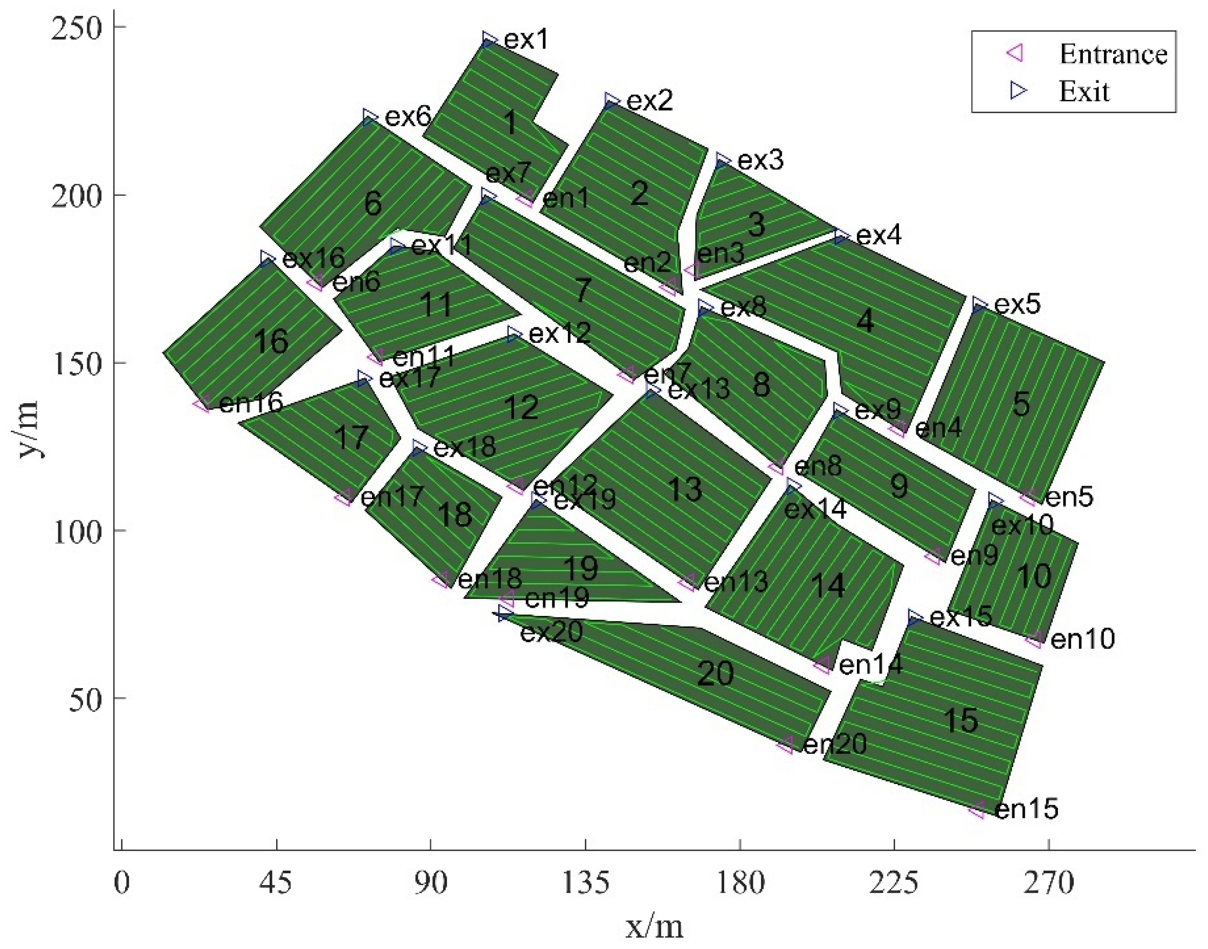
2. Harvester Field Operation Environment Model
2.1. Full Coverage Environment Modeling
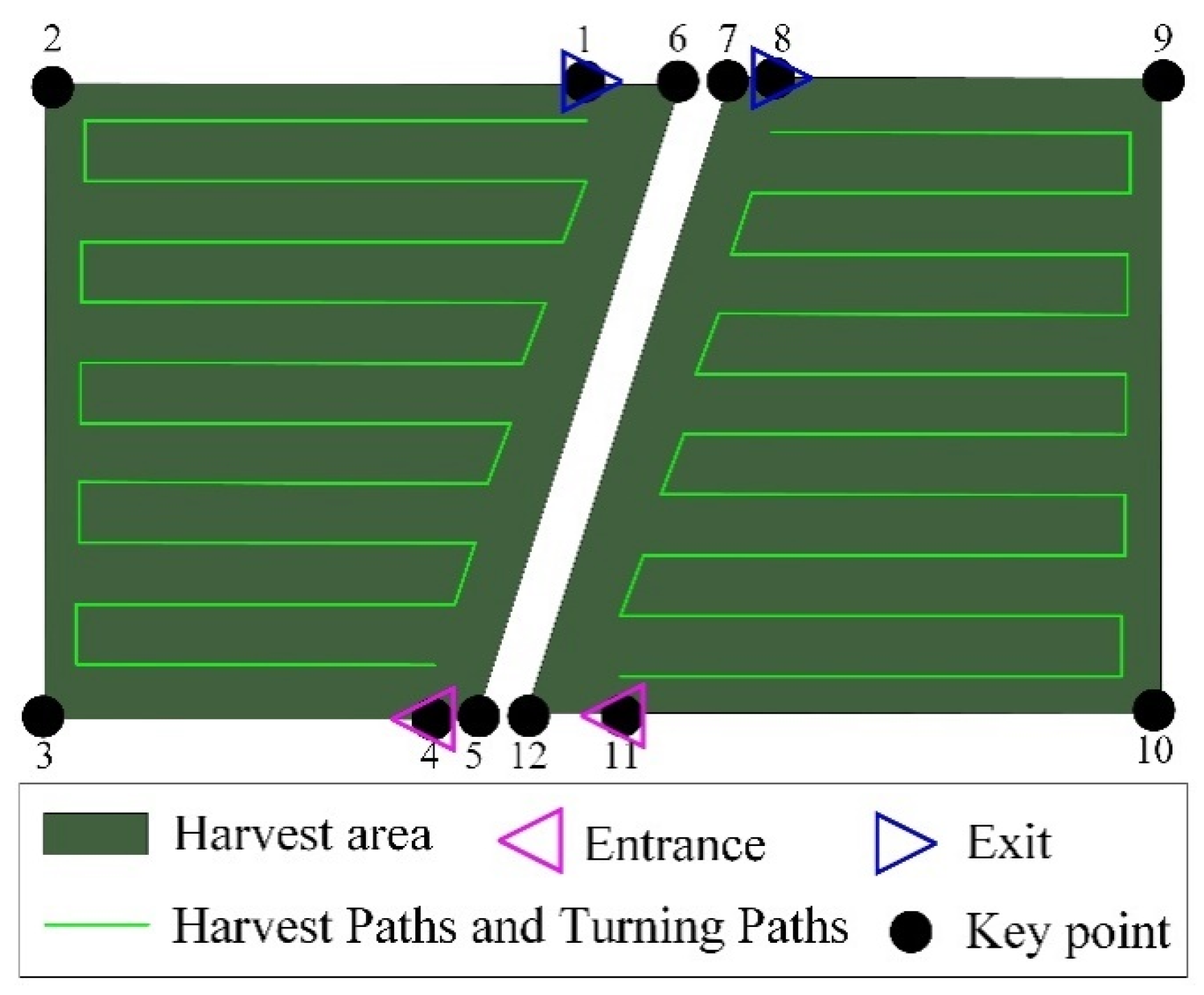
2.2. Full Coverage Path Planning for Harvester Field Operations
3. Multi-Field Connection Path Planning Based on Dijkstra’s Algorithm
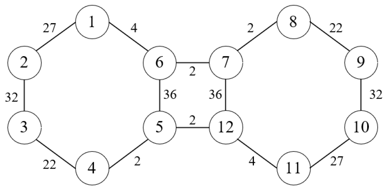
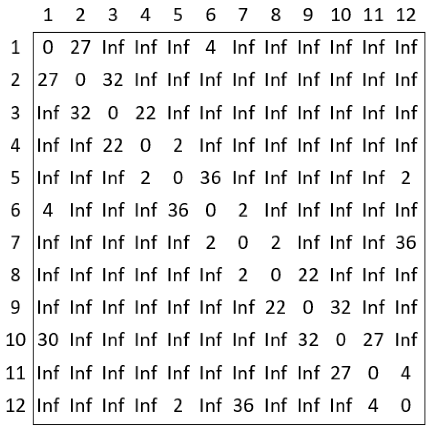
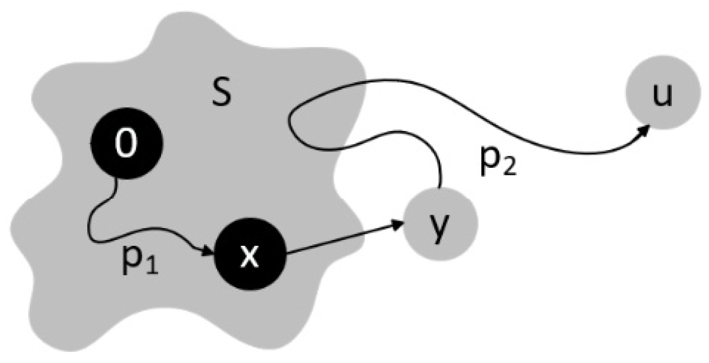
3.1. Design of Field Transfer Road Network Graph
3.2. Solving the Shortest Path Using Dijkstra’s Algorithm
3.3. Iterative Calculation
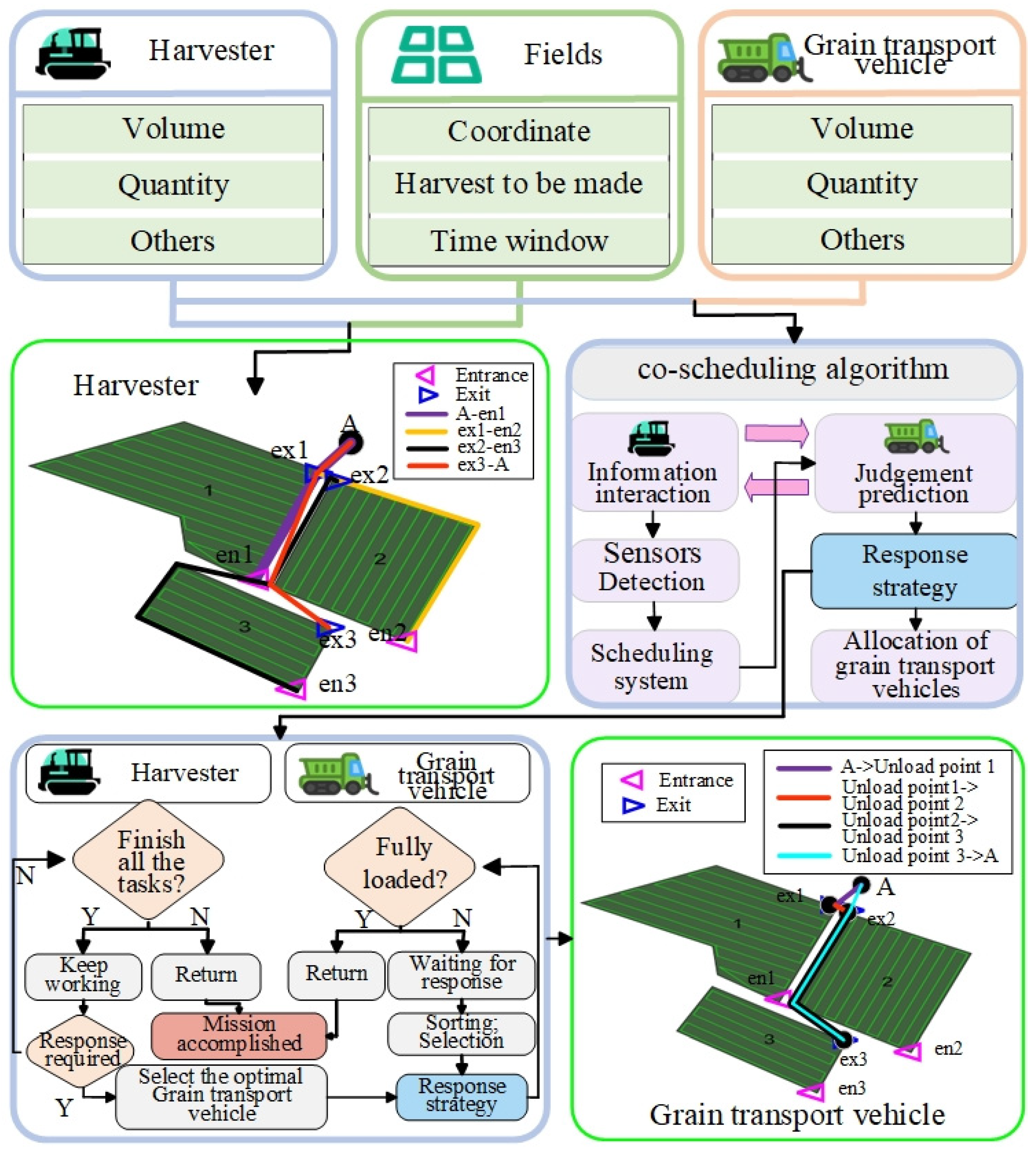
4. Collaborative Harvesting and Transport Scheduling Model
4.1. Problem Description
4.2. Grain Loading and Unloading Process
4.3. Assumptions and Conditions
- (1)
- Each farmland can be accessed by only one harvester and at least zero grain transport vehicles.
- (2)
- Both the harvester and grain transport vehicles depart from the machinery depot, returning to the depot after all tasks are completed, with the coordinates of the depot known.
- (3)
- The capacity and travel speed of both the harvester and grain transport vehicles are known.
- (4)
- The coordinates, time windows, and harvesting requirements for each farmland are known.
- (5)
- The maximum load capacity of the harvester and grain transport vehicle cannot exceed their respective capacities, and the grain transport vehicle must return to the machinery depot once fully loaded.
- (6)
- The grain transport vehicle can only move to key nodes to assist the harvester with loading and unloading grain.
- (7)
- The nearest key node to the position where the harvester is fully loaded is the unloading point.
- (8)
- The time, distance, and fuel consumption associated with the movement of the grain transport vehicle within the field are ignored.
- (9)
- It is assumed that there are no machinery failures or obstacles in the field during operations.
4.4. Collaborative Scheduling Model
4.5. Response Strategy
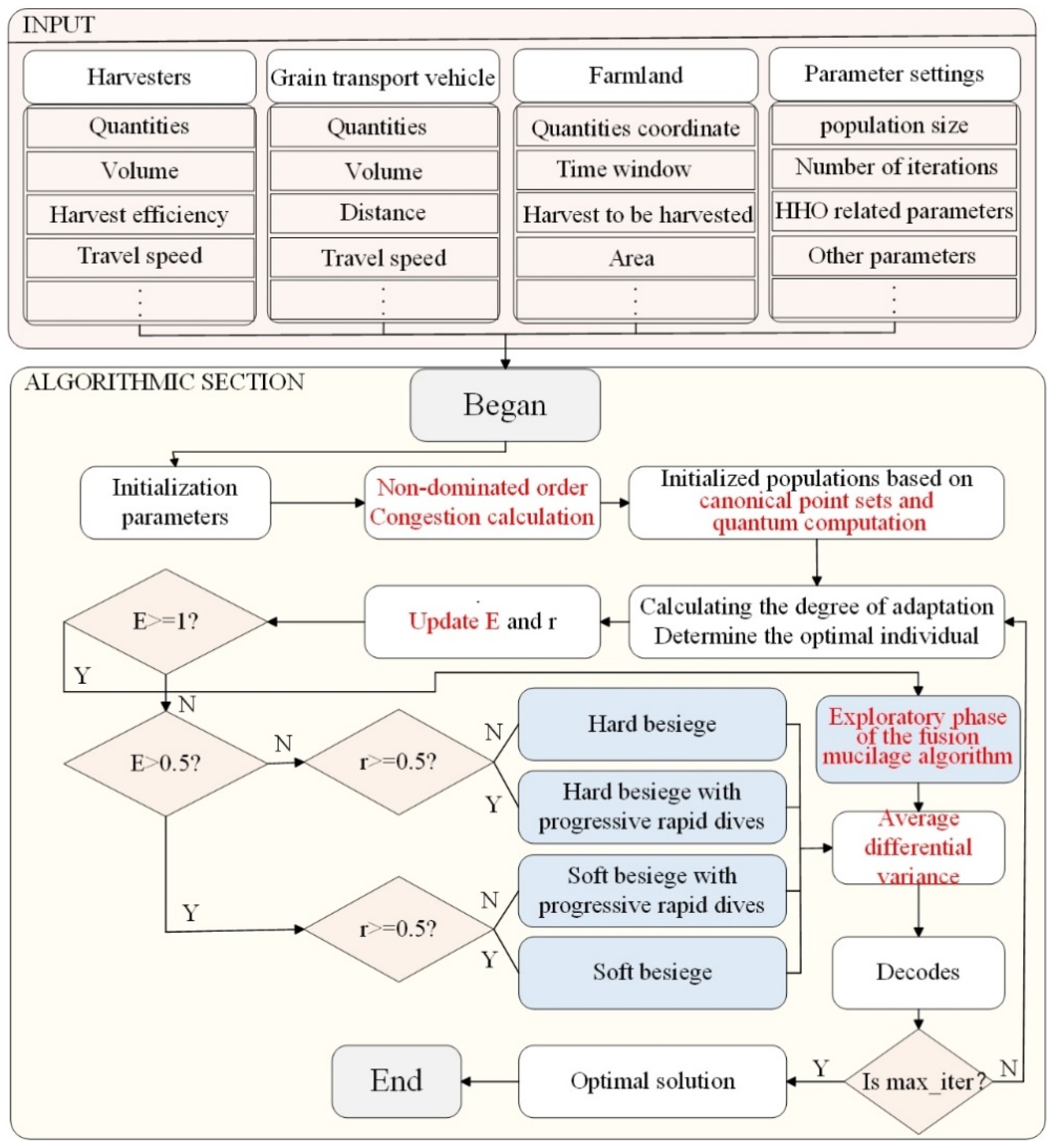
5. Collaborative Scheduling and Transportation Planning Based on IHHO
5.1. Model Solution Algorithm Design
5.2. Model Solution Process
- (1)
- Parameter setting: Basic parameters for farmlands, machinery storage, harvesters, and grain transport vehicles are set, along with the relevant parameters for the HHO algorithm and slime mold algorithm.
- (2)
- Encoding and decoding: A real-number encoding scheme is used. The state of each hawk is represented by a string of floating-point numbers between 0 and 1, where each number represents the fitness value for a particular farmland. The fitness value changes based on the distance between the hawk and its prey, as well as the current state of both the hawk and the prey. The decoding process converts the hawk’s state into a specific farmland allocation plan.
- (3)
- Best point set (BPS) and quantum computing initialization: In the traditional HHO algorithm, the initial population is generated randomly. However, this initialization process can lead to uneven population distribution, reducing population diversity, which significantly affects the quality of the initial solution and convergence speed. Therefore, the BPS method [24] is employed to generate effective and uniformly distributed points, thereby improving global search efficiency. Theoretical research [25] shows that a weighted sum of n best points leads to a smaller error than using any other set of n points, particularly in complex search spaces. Let Gs represent a unit cube in the s-dimensional Euclidean space, and if g ∈ Gs, as shown in Equation (18), then Pn(k) denotes the best point set, with g being the best point.
- (4)
- Objective function calculation: The HHO algorithm is typically a single-objective optimization algorithm, while the problem addressed in this study is a complex, multi-objective optimization problem, necessitating an extension of the HHO algorithm. However, multi-objective functions often conflict with one another, requiring the identification of a set of good solutions within the solution space. Therefore, a non-dominated sorting approach combined with a crowding distance mechanism to maintain diversity is employed. First, non-dominated solutions are calculated, followed by non-dominated sorting, and the non-dominated ranking of all solutions is computed. The crowding distance mechanism is then used to maintain diversity between solutions, ensuring that the diversity of solutions is effectively preserved during the optimization process. The crowding distance is defined as:
- (5)
- Fitness calculation: The fitness value of each Harris hawk individual is calculated, the best fitness value is recorded, and the position of the Harris hawk with the optimal fitness is set as the prey position.
- (6)
- Exploration phase with fused slime mold algorithm (SMA): To address the issue where HHO can easily get trapped in local optima when solving complex problems, the multiple search mechanism of the SMA is incorporated into the exploration phase of HHO to enhance its global search ability [29]. First, the exploration phase of HHO conducts a broad search for high-quality solutions in the solution space, as shown in Equation (25). Then, a local search is performed on the high-quality solutions using SMA’s approach strategies, including the proximity strategy (Equation (27)), encircling strategy (Equation (30)), and acquiring strategy. Specifically, the multiple search mechanism of SMA adjusts different search patterns based on fitness values, while also separating a portion of the organic matter to explore other domains. The oscillation effect between vb (simulating the interaction process of individual slime mold information) and vc (simulating the slime mold’s retention of its own information) causes the search direction of the slime mold to become more divergent, thus increasing the possibility of global exploration. The multiple exploration mechanism endows the algorithm with strong global optimization capabilities. Additionally, when rand < z (where z represents the probability that the slime mold separates individual agents to search for other food sources), a portion of the slime mold population is randomly generated in the solution space, simulating the behavior of slime mold individuals separating and exploring other potential food sources.
- (7)
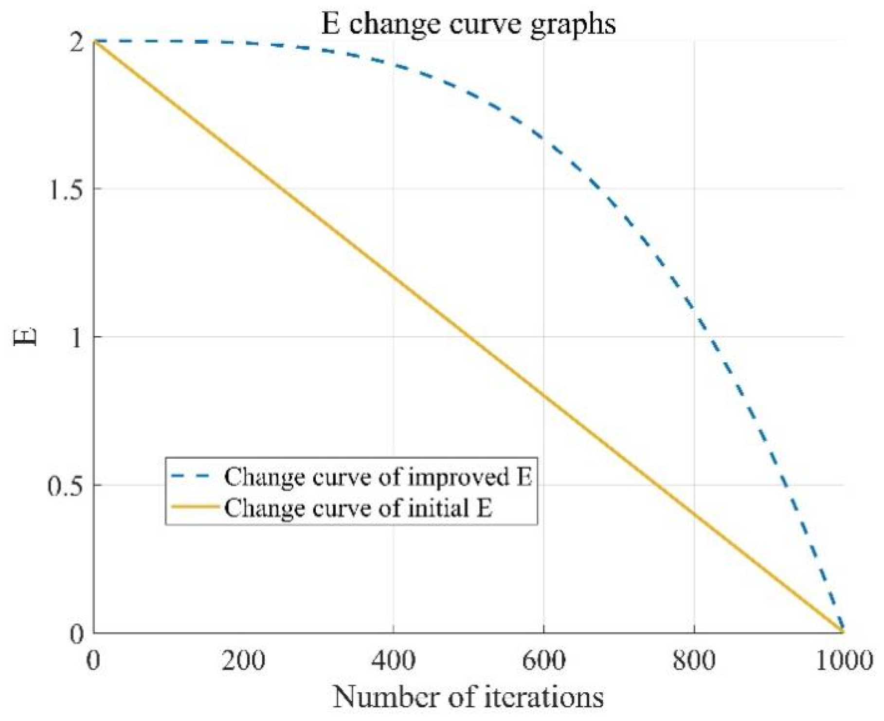
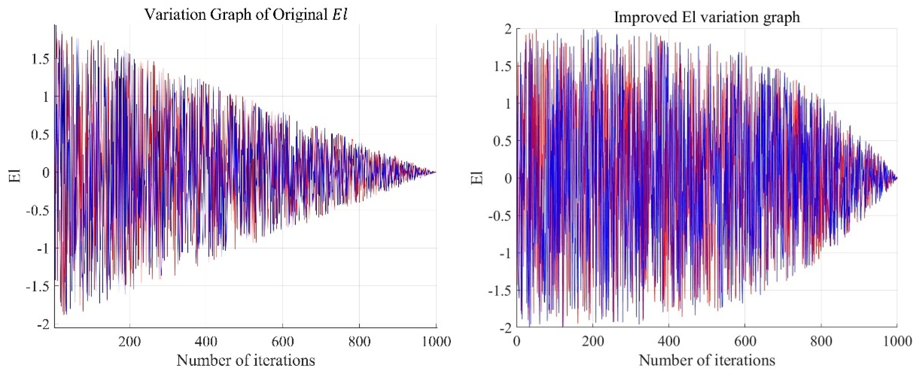
- Exploration and exploitation transition phase: A nonlinear prey escape energy update strategy is adopted. The key parameter that controls the exploration and exploitation phases (the global to local search transition) of the HHO algorithm is the prey escape energy El, as shown in Equation (31). If ∣El∣ ≥ 1, the algorithm enters the global search phase, i.e., the exploration phase. If ∣El∣ < 1, the algorithm enters the local search phase, i.e., the exploitation phase. The energy factor E is updated in a linear fashion from 2 to 0. Figure 9 illustrates the change in E over 1000 iterations. This linear decrease causes the algorithm to get trapped in local search during the later stages of iteration. To address this, a nonlinear energy factor update strategy, based on the experience in [30], is adopted, as shown in Equation (32). This strategy allows the algorithm to maintain the possibility of global search while performing local search in the later iterations. The parameter δ is set to 3.5. Figure 10 shows the variation in El over 1000 iterations. The improved El changes slowly in the early stages of the algorithm, enhancing the global search performance of HHO, while in the later stages, the reduction rate of El accelerates, improving the local search performance and search efficiency of the algorithm.
- (8)
- Development strategy: After locating the prey, the Harris hawk initiates an attack during the development phase by encircling the prey, waiting for an opportunity to strike. However, the actual hunting process is complex. For instance, a prey surrounded by the hawk may escape the encirclement, prompting the hawk to adjust its actions based on the prey’s behavior. Consequently, the HHO algorithm employs four strategies to mimic the hunting behavior of the Harris hawk. These strategies are soft encirclement, hard encirclement, progressive rapid dive with soft encirclement, and progressive rapid dive with hard encirclement.
- Soft encirclement when 0.5 ≤ ∣E∣ < 1 and r3 ≥ 0.5
- b.
- Hard encirclement when ∣E∣ < 0.5 and r3 ≥ 0.5
- c.
- Progressive rapid dive with soft encirclement when 0.5 ≤ ∣E∣ < 1 and r3 < 0.5
- d.
- Progressive rapid dive with hard encirclement when ∣E∣ < 0.5 and r3 < 0.5
- (9)
- Average difference mutation strategy: Due to the convergence of Harris hawks in the population towards the optimal individual during the iterative process, if there are local optima, Harris hawks tend to cluster around them as the number of iterations increases, which can lead to a reduction in population diversity. To avoid the algorithm getting trapped in local optima and prevent premature convergence, an average difference mutation [31] is introduced to adjust the individual and global best solutions.
- (10)
- Updating objective function and fitness values. After updating the objective function and fitness values, the individual with the maximum fitness is identified, and the fitness value is returned.
- (11)
- Iterative evolution. The algorithm checks whether it has reached the specified number of iterations. If so, the algorithm terminates, and the optimal result is decoded. Otherwise, the algorithm continues iterating. The pseudocode for the IHHO algorithm is shown in Algorithm 1.
| Algorithm 1. IHHO algorithm pseudocode |
| Input: The population size Popsize and maximum number of iterations Max_t |
| Output: Prey location and fitness values |
| Initialize the population using Equations (18) and (20)–(23) for the Canonical point set and quantum computation. |
| While termination criteria have not been satisfied do |
| Calculate the fitness values of hawks |
| Set Xprey as the location of prey (best location) |
| ))) do |
| Update the initial energy E0 and jump strength J |
| Update the E using Equation (32) |
| if (∣E ≥ 1∣) then ->Exploratory phase of the fusion mucilage algorithm |
| Update the location vector using Equations (25), (27) and (30). |
| if (∣E∣ < 1) then ->Exploitation phase |
| if (0.5 ≤ ∣E∣ < 1 and r3 ≥ 0.5) then ->Soft besiege |
| Update the location vector using Equation (34) |
| else if (∣E∣ < 0.5 and r3 ≥ 0.5) then ->Hard besiege |
| Update the location vector using Equation (36) |
| else if (0.5 ≤ ∣E∣ < 1 and r3 < 0.5) then ->Soft besiege with progressive rapid dives |
| Update the location vector using Equation (37) |
| else if (∣E∣ < 0.5 and r3 < 0.5) then ->Hard besiege with progressive rapid dives |
| Update the location vector using Equation (39) |
| Equation (41) was used for the mean difference variance strategy. |
| Return Xprey |
6. Example Studies
6.1. Experimental Data
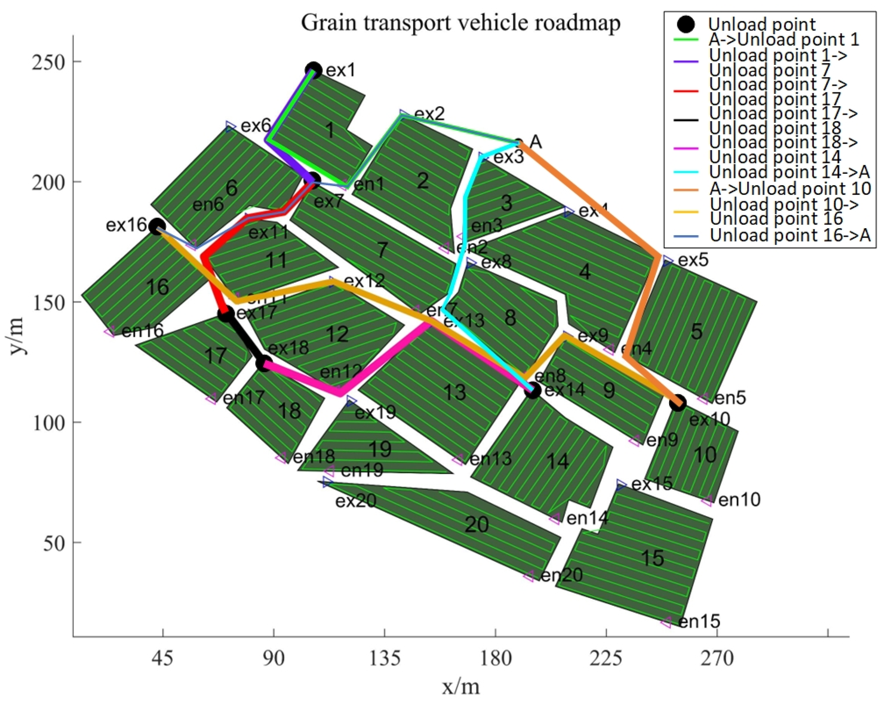
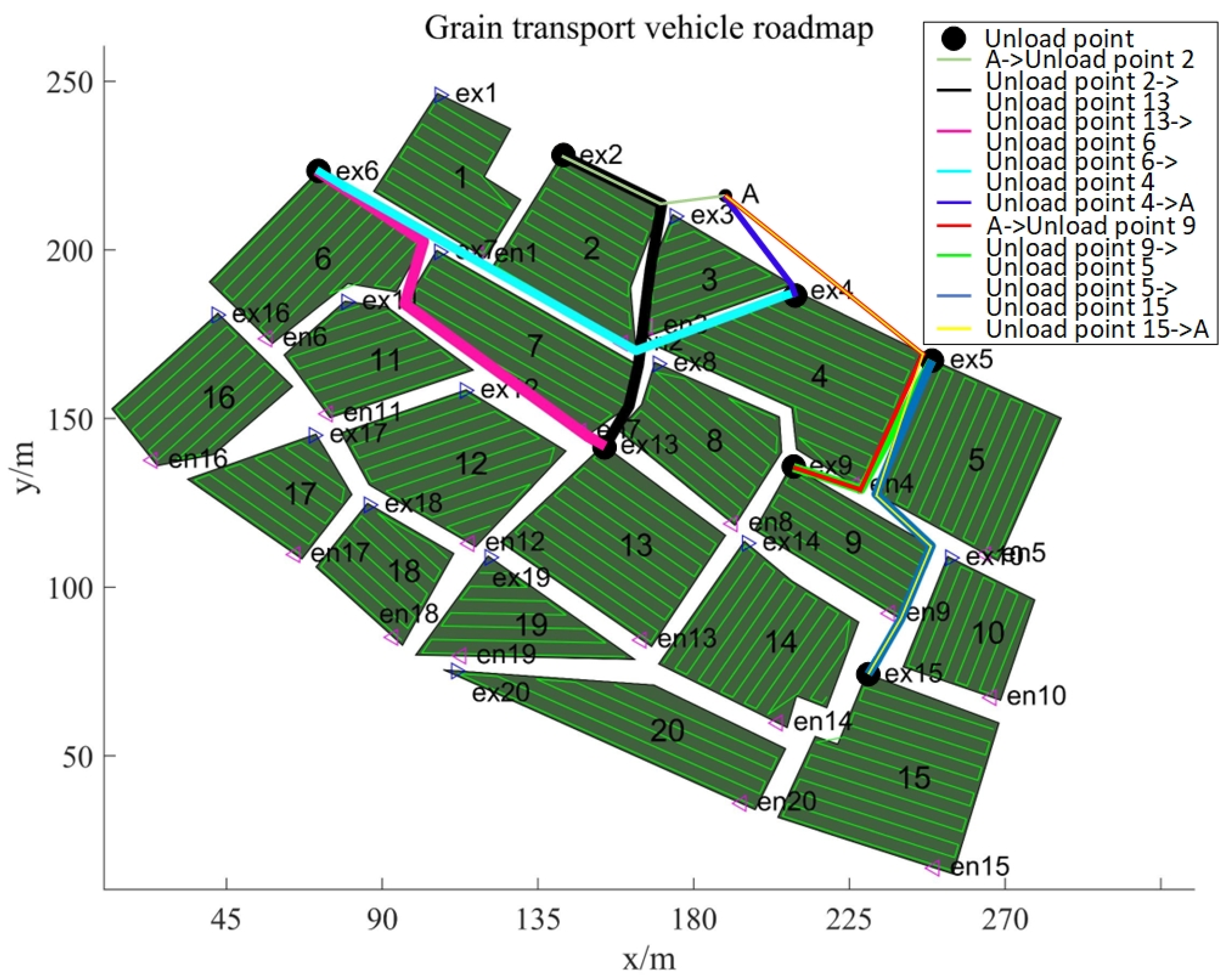
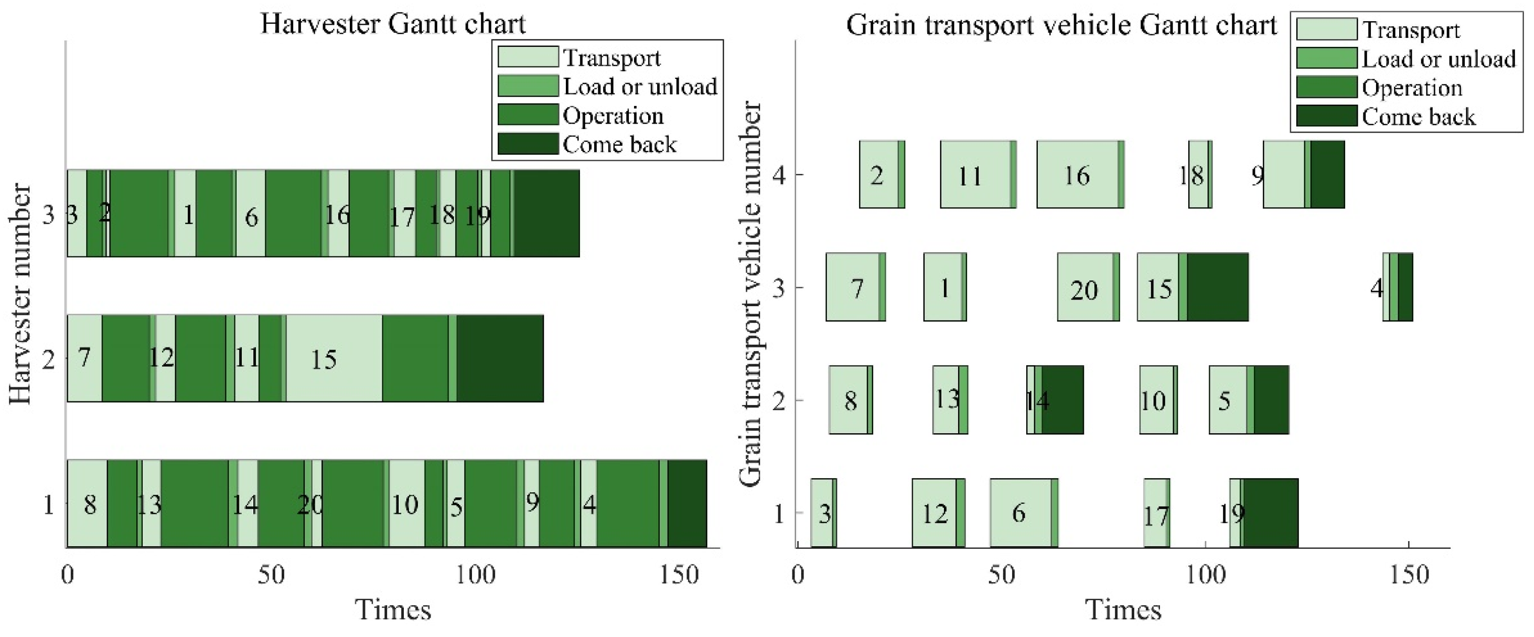
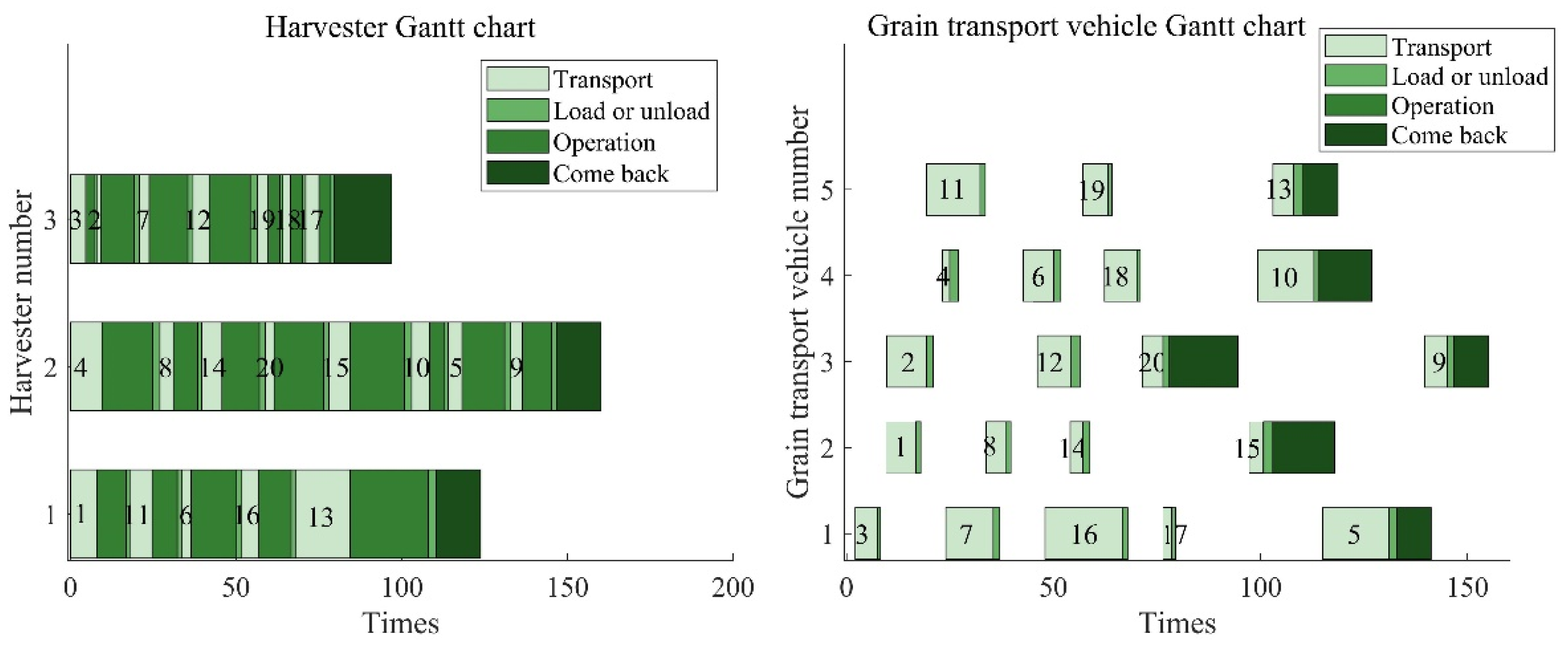
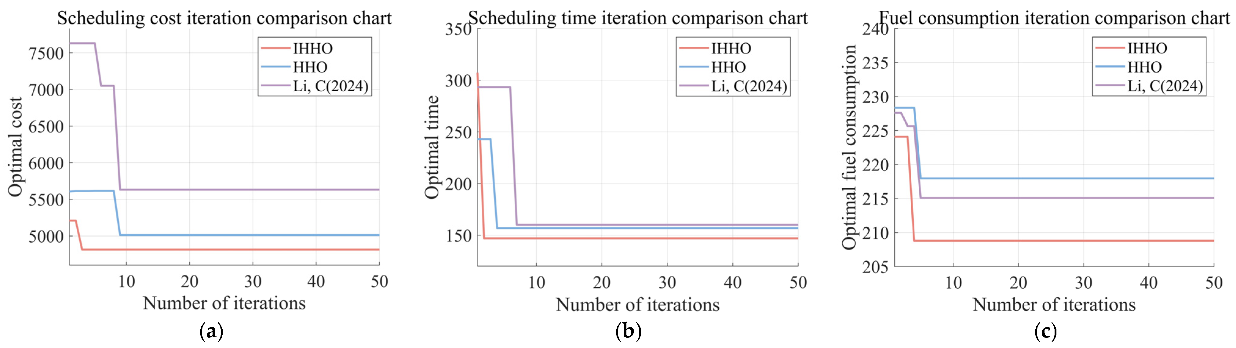
6.2. Experimental Results
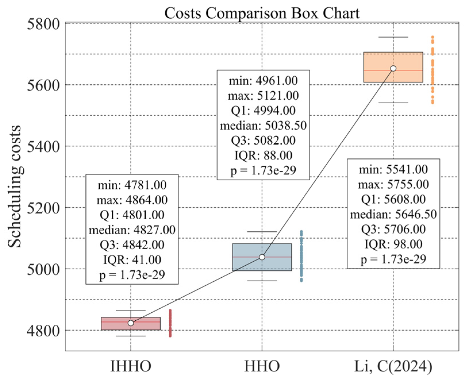
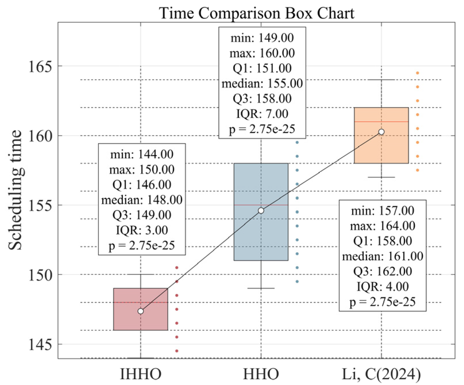
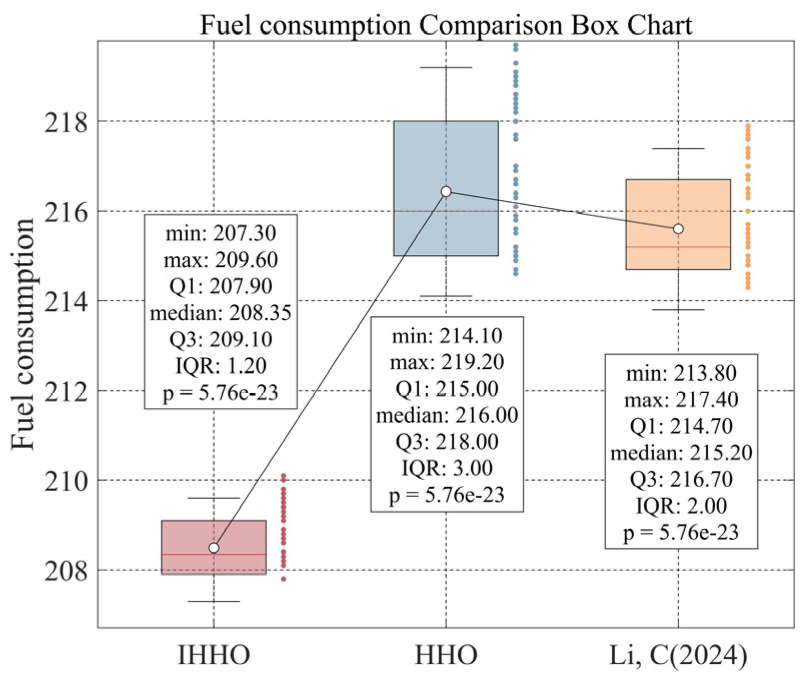
7. Statistical Analysis of the IHHO Algorithm
8. Conclusions
Author Contributions
Funding
Institutional Review Board Statement
Data Availability Statement
Acknowledgments
Conflicts of Interest
Appendix A

| No. | Scheduling Costs (CNY) | Scheduling Time (min) | Fuel Consumption (L) | No. | Scheduling Costs (CNY) | Scheduling Time (min) | Fuel Consumption (L) |
|---|---|---|---|---|---|---|---|
| 1 | 4819 | 147 | 208.8 | 26 | 4827 | 150 | 207.8 |
| 2 | 4851 | 146 | 209.5 | 27 | 4848 | 149 | 209.2 |
| 3 | 4855 | 147 | 208.4 | 28 | 4782 | 145 | 208.9 |
| 4 | 4819 | 144 | 207.9 | 29 | 4796 | 144 | 208.3 |
| 5 | 4801 | 146 | 209.3 | 30 | 4806 | 144 | 207.3 |
| 6 | 4828 | 150 | 209.6 | 31 | 4859 | 147 | 209.5 |
| 7 | 4794 | 149 | 209.3 | 32 | 4831 | 144 | 209.1 |
| 8 | 4838 | 150 | 209 | 33 | 4800 | 149 | 209.3 |
| 9 | 4805 | 146 | 208.8 | 34 | 4815 | 149 | 209.6 |
| 10 | 4852 | 144 | 209 | 35 | 4806 | 144 | 207.3 |
| 11 | 4824 | 148 | 208.3 | 36 | 4828 | 150 | 208.7 |
| 12 | 4800 | 148 | 208.3 | 37 | 4792 | 147 | 209.5 |
| 13 | 4792 | 148 | 208.7 | 38 | 4785 | 148 | 207.7 |
| 14 | 4841 | 149 | 209.1 | 39 | 4803 | 149 | 207.8 |
| 15 | 4855 | 146 | 208.2 | 40 | 4855 | 150 | 208.2 |
| 16 | 4847 | 146 | 208.1 | 41 | 4781 | 148 | 207.9 |
| 17 | 4839 | 150 | 207.3 | 42 | 4818 | 150 | 207.8 |
| 18 | 4846 | 144 | 208.4 | 43 | 4827 | 150 | 208.2 |
| 19 | 4830 | 147 | 207.8 | 44 | 4841 | 150 | 208.1 |
| 20 | 4828 | 145 | 208.4 | 45 | 4859 | 148 | 208.2 |
| 21 | 4859 | 149 | 208.3 | 46 | 4794 | 148 | 207.9 |
| 22 | 4864 | 150 | 208.2 | 47 | 4787 | 146 | 209.2 |
| 23 | 4796 | 144 | 207.6 | 48 | 4815 | 145 | 209.5 |
| 24 | 4837 | 145 | 208.6 | 49 | 4842 | 149 | 207.9 |
| 25 | 4804 | 149 | 208.8 | 50 | 4842 | 148 | 207.8 |
| No. | Scheduling Costs (CNY) | Scheduling Time (min) | Fuel Consumption (L) | No. | Scheduling Costs (CNY) | Scheduling Time (min) | Fuel Consumption (L) |
|---|---|---|---|---|---|---|---|
| 1 | 5012 | 157 | 217.9 | 26 | 5026 | 155 | 215.6 |
| 2 | 4991 | 156 | 215.6 | 27 | 4994 | 157 | 214.2 |
| 3 | 4966 | 155 | 218.4 | 28 | 4996 | 149 | 215.8 |
| 4 | 5060 | 149 | 214.4 | 29 | 5071 | 158 | 215.9 |
| 5 | 4983 | 159 | 214.7 | 30 | 4993 | 149 | 215 |
| 6 | 4963 | 155 | 218.1 | 31 | 4962 | 159 | 215.3 |
| 7 | 5113 | 149 | 218 | 32 | 5043 | 154 | 215.4 |
| 8 | 4987 | 152 | 215 | 33 | 5053 | 149 | 217.1 |
| 9 | 5012 | 152 | 217.7 | 34 | 5021 | 151 | 218.8 |
| 10 | 5067 | 149 | 215.6 | 35 | 5113 | 153 | 217.7 |
| 11 | 4996 | 158 | 217.5 | 36 | 5082 | 150 | 214.7 |
| 12 | 5044 | 158 | 216.4 | 37 | 5007 | 156 | 218.3 |
| 13 | 5120 | 158 | 218.8 | 38 | 5073 | 155 | 217.5 |
| 14 | 5120 | 159 | 214.1 | 39 | 4964 | 156 | 218.4 |
| 15 | 4963 | 155 | 218.6 | 40 | 5049 | 150 | 215.6 |
| 16 | 5121 | 158 | 219.2 | 41 | 5096 | 160 | 216.2 |
| 17 | 5099 | 149 | 218.3 | 42 | 5090 | 156 | 215.1 |
| 18 | 5028 | 154 | 215.3 | 43 | 5093 | 158 | 215.1 |
| 19 | 5114 | 152 | 214.2 | 44 | 5006 | 160 | 218.5 |
| 20 | 4961 | 154 | 216.5 | 45 | 5064 | 158 | 217.8 |
| 21 | 5034 | 159 | 217.2 | 46 | 5110 | 149 | 214.5 |
| 22 | 5001 | 153 | 214.6 | 47 | 5097 | 160 | 216.1 |
| 23 | 5041 | 149 | 214.1 | 48 | 5072 | 158 | 215.6 |
| 24 | 4978 | 156 | 214.7 | 49 | 5036 | 151 | 215 |
| 25 | 5062 | 160 | 219.1 | 50 | 4961 | 154 | 218.6 |
| No. | Scheduling Costs (CNY) | Scheduling Time (min) | Fuel Consumption (L) | No. | Scheduling Costs (CNY) | Scheduling Time (min) | Fuel Consumption (L) |
|---|---|---|---|---|---|---|---|
| 1 | 5633 | 160 | 215.1 | 26 | 5606 | 160 | 216.2 |
| 2 | 5541 | 162 | 216.7 | 27 | 5702 | 157 | 217.3 |
| 3 | 5738 | 159 | 217.1 | 28 | 5631 | 158 | 216.2 |
| 4 | 5619 | 162 | 214.7 | 29 | 5706 | 161 | 214 |
| 5 | 5674 | 162 | 215 | 30 | 5643 | 160 | 214.9 |
| 6 | 5699 | 159 | 214.5 | 31 | 5676 | 160 | 214.4 |
| 7 | 5663 | 161 | 217.1 | 32 | 5589 | 161 | 216 |
| 8 | 5642 | 161 | 215.1 | 33 | 5711 | 157 | 216.8 |
| 9 | 5614 | 158 | 217.4 | 34 | 5739 | 157 | 215.5 |
| 10 | 5743 | 162 | 216.5 | 35 | 5737 | 161 | 215.9 |
| 11 | 5603 | 162 | 216.7 | 36 | 5755 | 163 | 214.7 |
| 12 | 5608 | 157 | 216.7 | 37 | 5754 | 158 | 216.3 |
| 13 | 5678 | 157 | 217.2 | 38 | 5743 | 161 | 215.8 |
| 14 | 5619 | 161 | 214.8 | 39 | 5541 | 162 | 214.8 |
| 15 | 5674 | 159 | 213.8 | 40 | 5675 | 160 | 216.5 |
| 16 | 5608 | 164 | 214.9 | 41 | 5710 | 162 | 214.3 |
| 17 | 5547 | 163 | 214.4 | 42 | 5715 | 163 | 214.7 |
| 18 | 5667 | 160 | 216.7 | 43 | 5634 | 162 | 215.9 |
| 19 | 5672 | 157 | 214.7 | 44 | 5633 | 162 | 214.5 |
| 20 | 5623 | 161 | 213.9 | 45 | 5675 | 159 | 217.3 |
| 21 | 5650 | 164 | 214.1 | 46 | 5639 | 157 | 215 |
| 22 | 5578 | 157 | 215.2 | 47 | 5560 | 164 | 215 |
| 23 | 5717 | 157 | 214.4 | 48 | 5559 | 161 | 217.4 |
| 24 | 5713 | 163 | 216.9 | 49 | 5587 | 157 | 214.5 |
| 25 | 5632 | 164 | 215.2 | 50 | 5577 | 158 | 217.2 |
References
- Cao, R.; Guo, Y.; Zhang, Z.; Li, S.; Zhang, M.; Li, H.; Li, M. Global path conflict detection algorithm of multiple agricultural machinery cooperation based on topographic map and time window. Comput. Electron. Agric. 2023, 208, 107773. [Google Scholar] [CrossRef]
- Chen, M.; Xu, G.; Wei, Y.; Zhang, Y.; Diao, P.; Pang, H. Design and experiment analysis of the small maize harvester with attitude adjustment in the hilly and mountainous areas of China. Int. J. Agric. Biol. Eng. 2024, 17, 118–127. [Google Scholar] [CrossRef]
- Liu, H.; Zhang, L.; Zhao, B.; Tang, J.; Luo, J.; Wang, S. Research on Emergency Scheduling Based on Improved Genetic Algorithm in Harvester Failure Scenarios. Front. Plant Sci. 2024, 15, 1413595. [Google Scholar] [CrossRef] [PubMed]
- Liu, L.; Wang, X.; Liu, H.; Li, J.; Wang, P.; Yang, X. A Full-Coverage Path Planning Method for an Orchard Mower Based on the Dung Beetle Optimization Algorithm. Agriculture 2024, 14, 865. [Google Scholar] [CrossRef]
- Galarza-Falfan, J.; García-Guerrero, E.E.; Aguirre-Castro, O.A.; López-Bonilla, O.R.; Tamayo-Pérez, U.J.; Cárdenas-Valdez, J.R.; Hernández-Mejía, C.; Borrego-Dominguez, S.; Inzunza-Gonzalez, E. Path Planning for Autonomous Mobile Robot Using Intelligent Algorithms. Technologies 2024, 12, 82. [Google Scholar] [CrossRef]
- Gao, Y.; Han, Q.; Feng, S.; Wang, Z.; Meng, T.; Yang, J. Improvement and Fusion of D*Lite Algorithm and Dynamic Window Approach for Path Planning in Complex Environments. Machines 2024, 12, 525. [Google Scholar] [CrossRef]
- Shi, Y.; Huang, S.; Li, M. An Improved Global and Local Fusion Path-Planning Algorithm for Mobile Robots. Sensors 2024, 24, 7950. [Google Scholar] [CrossRef]
- Edwards, G.T.; Hinge, J.; Skou-Nielsen, N.; Villa-Henriksen, A.; Sørensen, C.A.; Green, O. Route planning evaluation of a prototype optimised infield route planner for neutral material flow agricultural operations. Biosyst. Eng. 2017, 153, 149–157. [Google Scholar] [CrossRef]
- Seyyedhasani, H.; Dvorak, J.S. Reducing field work time using fleet routing optimization. Biosyst. Eng. 2018, 169, 1–10. [Google Scholar] [CrossRef]
- Seyyedhasani, H.; Dvorak, J.S. Dynamic rerouting of a fleet of vehicles in agricultural operations through a Dynamic Multiple Depot Vehicle Routing Problem representation. Biosyst. Eng. 2018, 171, 63–77. [Google Scholar] [CrossRef]
- He, P.; Li, J. A joint optimization framework for wheat harvesting and transportation considering fragmental farmlands. Inf. Process. Agric. 2021, 8, 1–14. [Google Scholar] [CrossRef]
- Pan, W.; Wang, J.; Yang, W. A Cooperative Scheduling Based on Deep Reinforcement Learning for Multi-Agricultural Machines in Emergencies. Agriculture 2024, 14, 772. [Google Scholar] [CrossRef]
- Li, S.; Zhang, M.; Wang, N.; Cao, R.; Zhang, Z.; Ji, Y.; Li, H.; Wang, H. Intelligent scheduling method for multi-machine cooperative operation based on NSGA-III and improved ant colony algorithm. Comput. Electron. Agric. 2023, 204, 107532. [Google Scholar] [CrossRef]
- Chen, T.; Ahn, H.S.; Sun, W.; Pan, J.; Liu, Y.; Cheng, J.; Xu, L. Optimizing path planning for a single tracked combine harvester: A comprehensive approach to harvesting and unloading processes. Comput. Electron. Agric. 2024, 224, 109217. [Google Scholar] [CrossRef]
- Guo, Y.; Zhang, F.; Chang, S.; Li, Z.; Li, Z. Research on a multiobjective cooperative operation scheduling method for agricultural machinery across regions with time windows. Comput. Electron. Agric. 2024, 224, 109121. [Google Scholar] [CrossRef]
- Ptacek, M.; Frick, F.; Pahl, H.; Stetter, C.; Wimmer, S.; Sauer, J. ‘ShapeCostTUM’: A calculation tool for field geometry dependent cultivation and transport costs. Comput. Electron. Agric. 2024, 225, 109254. [Google Scholar] [CrossRef]
- Hameed, I.A. Intelligent coverage path planning for agricultural robots and autonomous machines on three-dimensional terrain. J. Intell. Robot. Syst. 2014, 74, 965–983. [Google Scholar] [CrossRef]
- Jaramillo-Martínez, R.; Chavero-Navarrete, E.; Ibarra-Pérez, T. Reinforcement-Learning-Based Path Planning: A Reward Function Strategy. Appl. Sci. 2024, 14, 7654. [Google Scholar] [CrossRef]
- Jia, J.; Tang, L. Optimal coverage path planning for arable farming on 2D surfaces. Trans. ASABE 2010, 53, 283–295. [Google Scholar]
- Shen, M.; Wang, S.; Wang, S.; Su, Y. Simulation study on coverage path planning of autonomous tasks in hilly farmland based on energy consumption model. Math. Probl. Eng. 2020, 2020, 4535734. [Google Scholar] [CrossRef]
- Nilsson, R.S.; Zhou, K. Method and benchmarking framework for coverage path planning in arable farming. Biosyst. Eng. 2020, 198, 248–265. [Google Scholar] [CrossRef]
- Gao, Y.; Ma, M.; Zhang, J.; Zhang, S.; Fang, J.; Gao, X.; Chen, G. Algorithms for Shortest Path Tour Problem in Large-Scale Road Network. In International Computing and Combinatorics Conference; Springer Nature: Cham, Switzerland, 2023. [Google Scholar] [CrossRef]
- Heidari, A.A.; Mirjalili, S.; Faris, H.; Aljarah, I.; Mafarja, M.; Chen, H. Harris hawks optimization: Algorithm and applications. Future Gener. Comput. Syst. 2019, 97, 849–872. [Google Scholar] [CrossRef]
- Yuan, J.; Liu, Z.; Lian, Y.; Chen, L.; An, Q.; Wang, L.; Ma, B. Global optimization of UAV area coverage path planning based on good point set and genetic algorithm. Aerospace 2022, 9, 86. [Google Scholar] [CrossRef]
- Devroye, L. Bounds for the uniform deviation of empirical measures. J. Multivar. Anal. 1982, 12, 72–79. [Google Scholar] [CrossRef]
- Kou, H.; Zhang, Y.; Lee, H.P. Dynamic optimization based on quantum computation-A comprehensive review. Comput. Struct. 2024, 292, 107255. [Google Scholar] [CrossRef]
- Du, Z.; Li, H. Research on Application of Improved Quantum Optimization Algorithm in Path Planning. Appl. Sci. 2024, 14, 4613. [Google Scholar] [CrossRef]
- Chauhan, J.; Alam, T. Adjustable rotation gate based quantum evolutionary algorithm for energy optimisation in cloud computing systems. Int. J. Comput. Sci. Eng. 2024, 27, 414–433. [Google Scholar] [CrossRef]
- Zhong, R.; Zhang, E.; Munetomo, M. Evolutionary multi-mode slime mold optimization: A hyper-heuristic algorithm inspired by slime mold foraging behaviors. J. Supercomput. 2024, 80, 12186–12217. [Google Scholar] [CrossRef]
- Uddin, M.P.; Majumder, A.; Barma, J.D.; Mirjalili, S. An Improved Multi-Objective Harris Hawks Optimization Algorithm for Solving EDM Problems. Arab. J. Sci. Eng. 2024, 1, 1–46. [Google Scholar] [CrossRef]
- Layeb, A. Differential evolution algorithms with novel mutations, adaptive parameters, and Weibull flight operator. Soft Comput. 2024, 28, 7039–7091. [Google Scholar] [CrossRef]
- Li, C.; Si, Q.; Zhao, J.; Qin, P. A robot path planning method using improved Harris Hawks optimization algorithm. Meas. Control 2024, 57, 469–482. [Google Scholar] [CrossRef]
- Yandrapalli, V. AI-Powered Data Governance: A Cutting-Edge Method for Ensuring Data Quality for Machine Learning Applications. In Proceedings of the 2024 Second International Conference on Emerging Trends in Information Technology and Engineering (ICETITE), Vellore, India, 22–23 February 2024. [Google Scholar] [CrossRef]
- McKight, P.E.; Najab, J. Kruskal-Wallis test. In The Corsini Encyclopedia of Psychology; John Wiley & Sons: Hoboken, NJ, USA, 2010; p. 1. [Google Scholar] [CrossRef]
- Mazarei, A.; Sousa, R.; Mendes-Moreira, J.; Molchanov, S. Online boxplot derived outlier detection. Int. J. Data Sci. Anal. 2024, 1, 1–15. [Google Scholar] [CrossRef]


| Symbols | Meaning |
|---|---|
| Estart | The fuel consumption during cold start: This refers to the fuel consumption of the harvester and grain transport vehicle when the engine has been turned off for a period of time, and the temperature has dropped below the normal operating temperature at the time of ignition. |
| Estart1 | Total startup fuel consumption: This refers to the fuel consumption during the process in which the engine reaches a stable minimum idle speed after starting. |
| Estart2 | Total idle fuel consumption: This refers to the fuel consumption during the process from parking to starting the movement of the vehicle. |
| Estart(h), Estart(g), | Harvester starting fuel consumption, grain transport vehicle starting fuel consumption. |
| Eidle(h), Eidle(g), | Harvester idling fuel consumption, grain transport vehicle idling fuel consumption. |
| tstart(h), tstart(g), | Harvester start time, grain transport vehicle start time. |
| tidle(h), tidle(g) | Harvester idle time, grain transport vehicle idle time. |
| Eflied | Fuel consumption of harvesters during field operations. |
| Ework | Fuel consumption during harvesting in the field. |
| Eturn | Fuel consumption during turning in the field. |
| Ehf | Fuel consumption of harvesters h during harvesting. |
| lhf | The number of rows harvested by harvester h in field f. |
| Df | Distance per row in farmland f. |
| Eh | Fuel consumption of harvester h during empty runs. |
| qhf | The number of turns made by harvester h within a farm field f. |
| Dh | Turning distance of harvester h. |
| dij | Distance from node i to node j. |
| Eschedue | Total scheduling fuel consumption: fuel consumption generated by the movement of the harvester and the grain transport vehicle in the field. |
| Esh Esg | Fuel consumption for scheduling of harvester h. Fuel consumption for scheduling of grain transport vehicle g. |
| dhf-en | Distance from the entrance of the field to the starting point of harvesting for harvester h. |
| dhf-ex | Distance from the end point of harvesting to the exit of the field for harvester h. |
| Eallot | Empty run fuel consumption: fuel consumption generated by the harvester from the entrance of the field to the starting position of harvesting and from the end position of harvesting to the exit of the field. |
| Cd | Distance cost between the harvester h and the grain transport vehicle g. |
| Cf | Fixed costs (scheduling cost costs). |
| Cp | Total penalty cost for violating time windows. |
| dc | Unit distance travel cost. |
| Ch,Cg | Scheduling costs for harvester h and grain transport vehicle g. |
| Pthg | Penalty cost for violating time windows. |
| Th | Maximum time Th taken to complete all tasks among all harvesters. |
| Tg | Maximum time Tg taken to complete all tasks among all grain transport vehicles. |
| Uh,Lg | Unloading time and loading time, where Uh = Lg. |
| Vh,Vg | Movement speeds of harvester h and grain transport vehicle g. |
| th | Harvesting time of harvester h for field f. |
| Hv,Gv | Capacity of harvesters, capacity of grain transport vehicles. |
| qf | The amount of farmland f to be harvested. |
| Di | Planting density of farmland f. |
| Ueh | Grain unloading efficiency of harvester h. |
| Cw,Cl | Cost of waiting per unit of time, cost of penalization per unit of time. |
| Bi,Ei | Time allowed for the start of the task on the farmland f and the latest time. |
| thgf | The moment the harvester or grain transport vehicle arrives on the farmland f. |
| Xijh,Xijg | Decision variable: a binary variable indicating whether harvester h or grain transport vehicle g travels from node i to node j. |
| Algorithm Parameter Setting | |
|---|---|
| Max_t ← 50 | % Number of iterations |
| Popsize ← 20 | % Population size |
| ub ← 10 | % Upper bound |
| lb ← −10 | % Lower bound |
| dim ← 30 | % Dimension |
| nq ← 4 | % Number of quantum bits |
| Experimental Parameter Setting | |
|---|---|
| Vh ← 10 | % Harvester travel speed |
| Vg ← 10 | % Grain transport vehicle travel speed |
| Hv ← [1000, 1700] | % Harvesters capacity |
| Gv ← 4000 | % Grain transport vehicle capacity |
| Ueh ← [50/3, 85/3] | % Harvester unit unloading efficiency(m3/min) |
| gn ← 10 | % Harvest per unit area |
| hc ← [300, 400] | % Harvester transfer, maintenance and fuel costs |
| gc ← 600 | % Transfers, maintenance and fuel costs for grain transport vehicles |
| dc ← 1 | % Cost per unit distance traveled |
| Cw ← 1 | % Cost of waiting per unit of time |
| Cl ← 1 | % Unit time penalty cost |
| Name | Volume (kg) | Model | Maximum Usage |
|---|---|---|---|
| Wode 4LZ-8.0EZ(Q) crawler corn harvester | 1700 | 4LZ-8.0EZ(Q) (China Jining Fengtuo Machinery Technology Co., Jining, China) | 5 |
| Huishou 4YZP-2D crawler two row corn harvester | 1000 | 4YZP-2D (China Shenyinong (Shandong) Agricultural Equipment Co., Weifang, China) | 5 |
| Jinan jinwang JW-4t crawler grain transport vehicle | 4000 | JW-4t (China Jining Jinwang Machinery Equipment Co., Jining, China) | 5 |
| Fields No. | Area/m2 | Harvest to Be Harvested /m3 | Time Window |
|---|---|---|---|
| A | / | / | [0, 1000] |
| 1 | 1073 | 536.5 | [242, 580] |
| 2 | 1450 | 725 | [160, 859] |
| 3 | 722 | 361 | [613, 771] |
| 4 | 1963 | 981.5 | [381, 651] |
| 5 | 1724 | 862 | [273, 625] |
| 6 | 1485 | 742.5 | [645, 809] |
| 7 | 1448 | 724 | [506, 950] |
| 8 | 1182 | 591 | [562, 900] |
| 9 | 1360 | 680 | [280, 920] |
| 10 | 915 | 457.5 | [659, 740] |
| 11 | 1190 | 595 | [94, 885] |
| 12 | 1921 | 960.5 | [366, 555] |
| 13 | 2117 | 1058.5 | [288, 655] |
| 14 | 1638 | 819 | [441, 875] |
| 15 | 2040 | 1020 | [605, 925] |
| 16 | 1194 | 597 | [513, 777] |
| 17 | 844 | 422 | [563, 790] |
| 18 | 818 | 409 | [815, 1111] |
| 19 | 896 | 448 | [340, 888] |
| 20 | 1415 | 707.5 | [886, 999] |
| Harvester Routes | Grain Transport Vehicle Routes | |
|---|---|---|
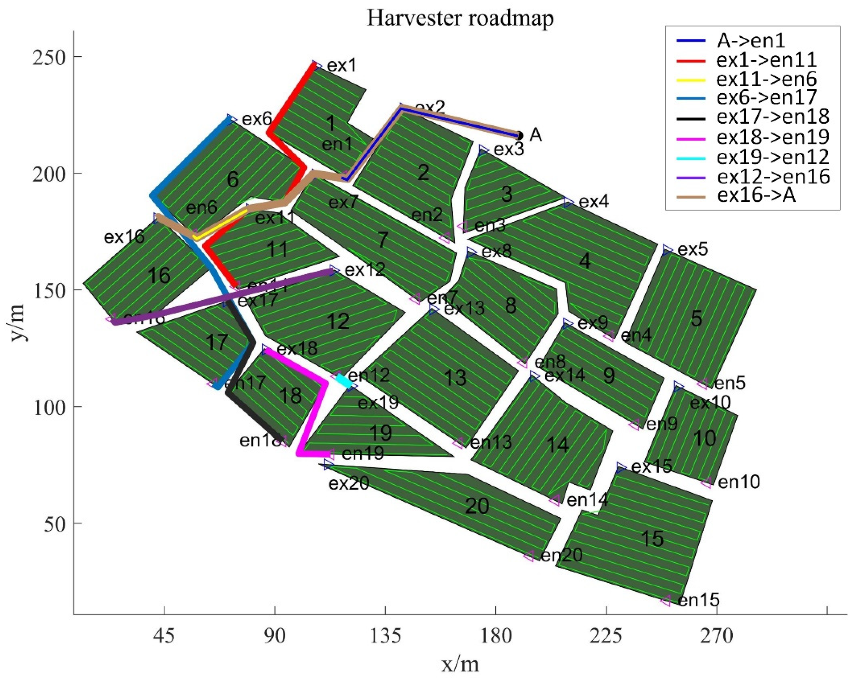
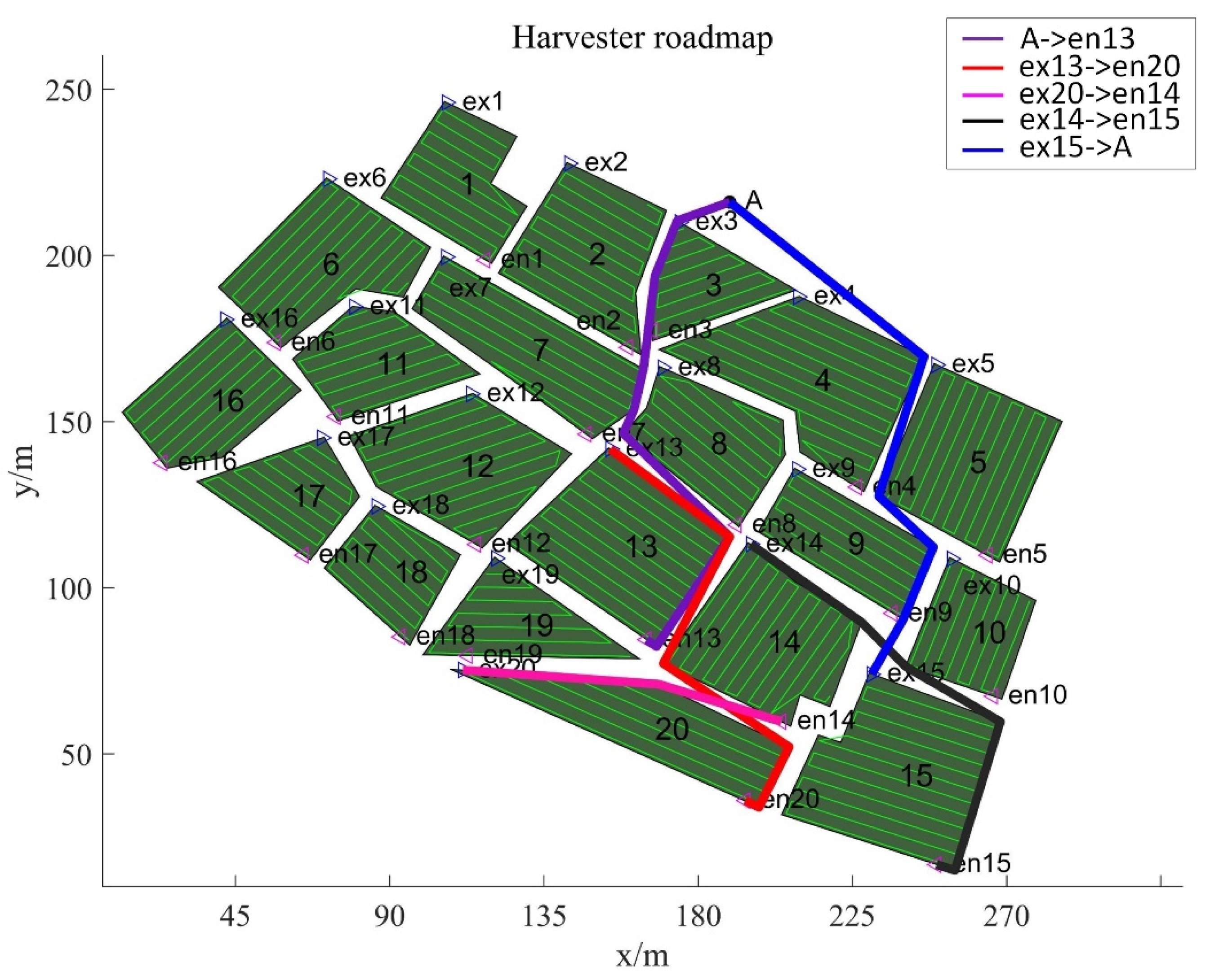
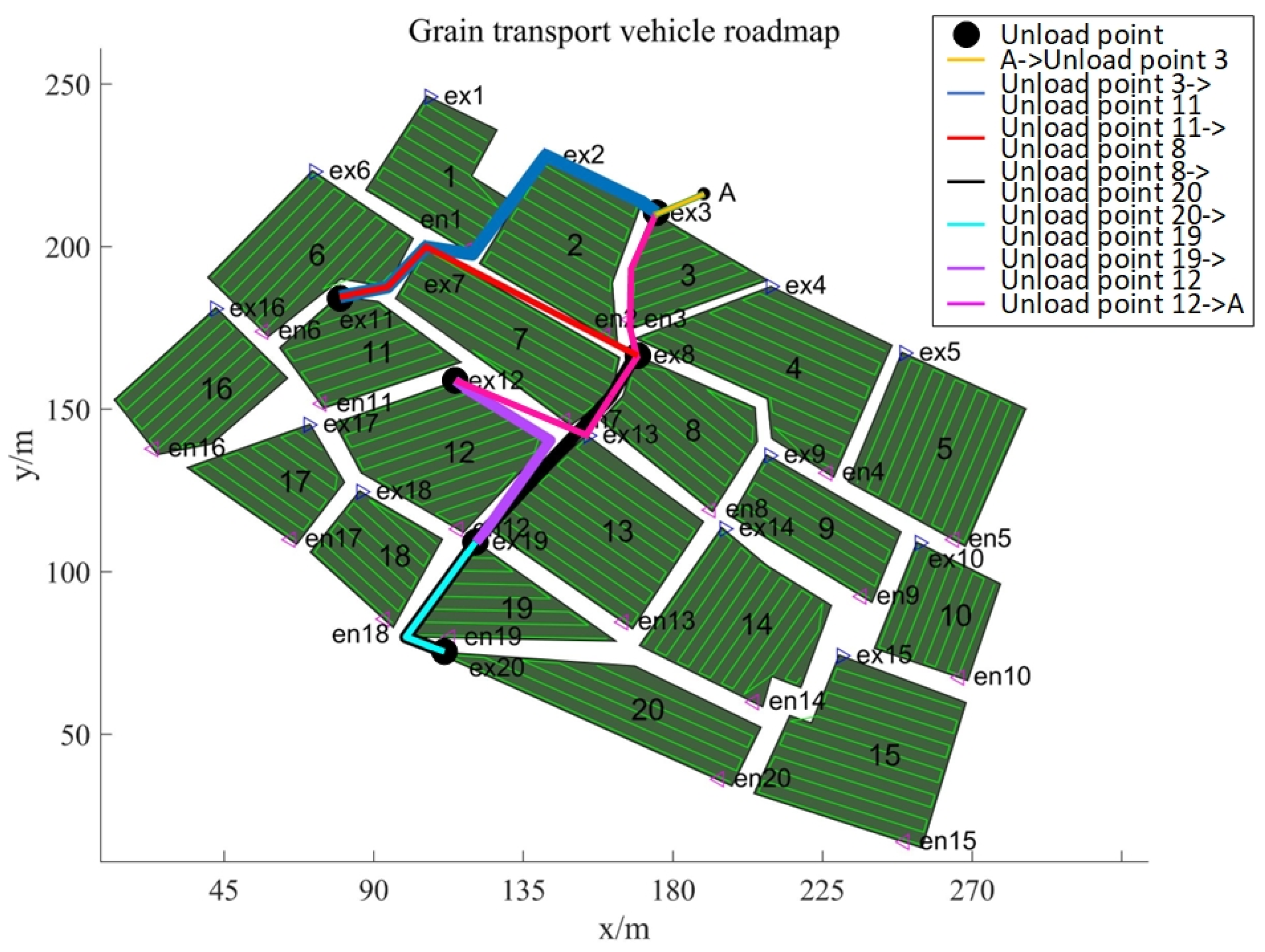
| IHHO | H1(V1200): A->1->11->6->17->18->19->12->16->A H2(V1200): A->13->20->14->15->A H3(V1700): A->3->2->7->8->4->9->5->10->A | G1: A->3->11->8->20->19->12->A G2: A->1->7->17->18->14->A->10->16->A G3: A->2->13->6->4->A->9->5->15->A |
| HHO | H1(V1700): A->8->13->14->20->10->5->9->4->A H2(V1700): A->7->12->11->15->A H3(V1200): A->3->2->1->6->16->17->18->19->A | G1: A->3->12->6->17->19->A G2: A->8->13->14->A->10->5->A G3: A->7->1->20->15->A->4->A G4: A->2->11->16->18->9->A |
| HHO algorithm in the literature [32] | H1(V1700): A->1->11->6->16->13->A H2(V1200): A->4->8->14->20->15->10->5->9->A H3(V1200): A->3->2->7->12->19->18->17->A | G1: A->3->7->16->17->5->A G2: A->1->8->14->15->A G3: A->2->12->20->A->9->A G4: A->4->6->18->10->A G5: A->11->19->13->A |
| Scheduling Costs (CNY) | Scheduling Time (min) | Fuel Consumption (L) | |
|---|---|---|---|
| IHHO | 4819 | 147 | 208.8 |
| HHO | 5012 | 157 | 217.9 |
| HHO algorithm in the literature [32] | 5633 | 160 | 215.1 |
Disclaimer/Publisher’s Note: The statements, opinions and data contained in all publications are solely those of the individual author(s) and contributor(s) and not of MDPI and/or the editor(s). MDPI and/or the editor(s) disclaim responsibility for any injury to people or property resulting from any ideas, methods, instructions or products referred to in the content. |
© 2025 by the authors. Licensee MDPI, Basel, Switzerland. This article is an open access article distributed under the terms and conditions of the Creative Commons Attribution (CC BY) license (https://creativecommons.org/licenses/by/4.0/).
Share and Cite
Liu, H.; Luo, J.; Zhang, L.; Yu, H.; Liu, X.; Wang, S. Research on Traversal Path Planning and Collaborative Scheduling for Corn Harvesting and Transportation in Hilly Areas Based on Dijkstra’s Algorithm and Improved Harris Hawk Optimization. Agriculture 2025, 15, 233. https://doi.org/10.3390/agriculture15030233
Liu H, Luo J, Zhang L, Yu H, Liu X, Wang S. Research on Traversal Path Planning and Collaborative Scheduling for Corn Harvesting and Transportation in Hilly Areas Based on Dijkstra’s Algorithm and Improved Harris Hawk Optimization. Agriculture. 2025; 15(3):233. https://doi.org/10.3390/agriculture15030233
Chicago/Turabian StyleLiu, Huanyu, Jiahao Luo, Lihan Zhang, Hao Yu, Xiangnan Liu, and Shuang Wang. 2025. "Research on Traversal Path Planning and Collaborative Scheduling for Corn Harvesting and Transportation in Hilly Areas Based on Dijkstra’s Algorithm and Improved Harris Hawk Optimization" Agriculture 15, no. 3: 233. https://doi.org/10.3390/agriculture15030233
APA StyleLiu, H., Luo, J., Zhang, L., Yu, H., Liu, X., & Wang, S. (2025). Research on Traversal Path Planning and Collaborative Scheduling for Corn Harvesting and Transportation in Hilly Areas Based on Dijkstra’s Algorithm and Improved Harris Hawk Optimization. Agriculture, 15(3), 233. https://doi.org/10.3390/agriculture15030233