Article

Identification of Cotton Leaf Mite Damage Stages Using UAV Multispectral Images and a Stacked Ensemble Method

1
College of Information and Management Science, Henan Agricultural University, Zhengzhou 450002, China
2
Institute of Plant Protection, Chinese Academy of Agricultural Sciences, Beijing 100193, China
3
Division of Pest Monitoring and Forecasting, National Agricultural Technology Service Center, Beijing 100125, China
*
Author to whom correspondence should be addressed.
Agriculture 2025, 15(21), 2277; https://doi.org/10.3390/agriculture15212277
Submission received: 13 October 2025 / Revised: 28 October 2025 / Accepted: 30 October 2025 / Published: 31 October 2025
(This article belongs to the Section Artificial Intelligence and Digital Agriculture)

Abstract

Cotton leaf mites are pests that cause irreparable damage to cotton and pose a severe threat to the cotton yield, and the application of unmanned aerial vehicles (UAVs) to monitor the incidence of cotton leaf mites across a vast region is important for cotton leaf mite prevention. In this work, 52 vegetation indices were calculated based on the original five bands of spliced UAV multispectral images, and six featured indices were screened using Shapley value theory. To classify and identify cotton leaf mite infestation classes, seven machine learning classification models were used: random forest (RF), support vector machine (SVM), extreme gradient boosting (XGB), light gradient boosting machine (LGBM), K-Nearest Neighbors (KNN), decision tree (DT), and gradient boosting decision tree (GBDT) models. The base model and metamodel used in stacked models were built based on a combination of four models, namely, the XGB, GBDT, KNN, and DT models, which were selected in accordance with the heterogeneity principle. The experimental results showed that the stacked classification models based on the XGB, KNN base model, and DT metamodel were the best performers, outperforming other integrated and single individual models, with an overall accuracy of 85.7% (precision: 93.3%, recall: 72.6%, and F1-score: 78.2% in the macro_avg case; precision: 88.6%, recall: 85.7%, and F1 score: 84.7% in the weighted_avg case). This approach provides support for using UAVs to monitor the cotton leaf mite prevalence over vast regions.

1. Introduction

Worldwide, cotton is a significant cash crop, and China is one of the largest cotton producers. Xinjiang is China’s largest cotton-growing province and industrial hub, producing 20% of the world’s cotton and 85% of the national total. In 2021, Xinjiang produced 5.129 million tons of cotton [1]. One of the most damaging and pervasive pests is the cotton leaf mite, which inhibits the sustainable growth of cotton in Xinjiang by causing an average yearly production loss of approximately 15–20% [2,3]. Monitoring the level of cotton leaf mite incidence is significant for the economic and agricultural sustainability of cotton crops, as well as for yield security.
To estimate the extent of cotton leaf mite incidence, manual ground surveys have traditionally been used. Due to the tiny size of cotton leaves, the survey procedure is often only effective in strong sunny areas, making the process costly, labor intensive, and time consuming. Drones, machine learning, and remote sensing technology have all advanced in recent years, and low-altitude drone-based remote sensing can be used to swiftly and correctly monitor pests and diseases in crop fields and provide useful information for yield prediction and planting management [4]. Using UAV multispectral imagery, Zhang et al. [5] achieved an overall accuracy of 97.28% for detecting banana Fusarium wilt through supervised and unsupervised classification methods, with the random forest model performing best among all approaches. A single boll was recognized and extracted using a complete convolutional network based on multitemporal visible cotton images obtained by a UAV. The single boll yield for each period was then forecasted using BP and partial least squares regression, with R2 values reaching 0.8162 and 0.8170, respectively [6]. Additionally, the hail ground vegetation index (HGVI) was established based on UAV multispectral images after cotton experienced hail damage during the boll stage. The kappa coefficient for classifying cotton hail damage based on the HGVI was greater than 0.85, indicating the viability of using UAV multispectral images to evaluate cotton damage due to hail [7]. Huang et al. [8] achieved an overall accuracy of 92.6% and an F-score of 0.976 for early-season cotton field identification by integrating Random Forest classification with 10-band Sentinel-2 imagery and field boundary data. Ren et al. [9] demonstrated that using UAV pan-sharpened multispectral imagery combined with a GBDT model achieved an R2 of 0.88 and an RMSE of 0.0918 for cotton aphid damage estimation, showing that image fusion significantly improves monitoring accuracy and efficiency compared with single multispectral imagery. The aforementioned studies demonstrate that because of their ease of use, flexibility, low cost, and excellent resolution, UAVs provide reliable hardware support for agricultural pest diagnosis. Notably, UAV systems offer the ability to obtain large-scale, high-resolution multispectral data suitable for monitoring cotton pest dynamics in Xinjiang [10].
Ali et al. [11] achieved an overall accuracy of 98% in detecting cotton leaf curl disease (CLCuD) by combining InceptionV3 and YOLOv8 models, demonstrating superior performance in early and accurate disease identification. Another researcher employed ResNet34 with a deep residual learning strategy to automatically identify important pests from UAV RGB photos. This method yielded an F-value of 0.98 and the highest classification accuracy among various convolutional networks and the traditional ResNet34 [12]. However, deep learning methods, although powerful, require large labeled datasets and high computing resources, which limit their feasibility for on-farm applications. In contrast, classical machine learning algorithms (e.g., RF, SVM, XGB, and LGBM) have demonstrated high efficiency and accuracy for multispectral data interpretation using smaller datasets and lower computational costs [13]. For instance, Pandiyaraju et al. [14] proposed spatial attention-based hybrid VGG-SVM and VGG-RF models for cotton leaf disease detection, achieving accuracies of 99.31% and 98.29%, respectively, outperforming existing state-of-the-art methods. Six machine learning algorithms were used to estimate the nitrogen nutrient index (NNI) and vegetation index of rice using drone RGB images taken at various stages of fertility. A random forest (RF) model performed the best, with a coefficient of determination (R2) between 0.88 and 0.96 and a root mean square error (RMSE) between 0.03 and 0.07, indicating that drone RGB information provides a basis for the rapid determination of the NNI of rice [15]. Nevertheless, single machine learning models often exhibit unstable generalization performance under different vegetation conditions. To overcome this limitation, ensemble learning approaches, particularly stacking, have been proposed to integrate multiple base models and improve classification robustness and accuracy [16,17,18,19,20,21]. To achieve effective pest monitoring, it is essential to integrate UAV-based image acquisition hardware with advanced algorithms capable of accurately interpreting multispectral data.
Building upon these advances, this study integrates UAV-based hardware for multispectral image acquisition with advanced software algorithms for data analysis. An integrated stacked model was developed to construct a classifier that effectively captures the spectral and textural characteristics of cotton leaf mites. Specifically, we used a UAV to collect multispectral images of cotton leaf mites in the study area. We then processed the images, applied SHAP value theory to filter the feature indices, used seven machine learning models for classification, and constructed stacked ensemble models to identify the severity levels of mite infestation. Compared with previous studies that mainly focused on binary classification of pest infestation—distinguishing only between healthy and infested leaves—this study advances toward a more refined multi-level classification of cotton leaf mite infestation using UAV multispectral imagery. Furthermore, the integration of interpretable SHAP-based feature selection with a stacked ensemble framework composed of heterogeneous base learners (XGB, GBDT, KNN, and DT) is expected to enhance classification accuracy, stability, and interpretability in a data-driven and explainable manner. This study provides a comprehensive and data-driven framework that bridges UAV sensing technology with interpretable ensemble learning to enable fine-grained, scalable pest monitoring and support early warning, precision pest control, and sustainable cotton production management.

2. Materials and Methods

2.1. Study Area

Figure 1 illustrates the location of the experiment, which was conducted at the Institute of Plant Protection’s Kulle base, Chinese Academy of Agricultural Sciences, in Kulle, Xinjiang (N 41°44′59″, E 85°48′30″). With the Tianshan Mountains to the north and the Tarim Basin to the south, Kulle is situated in the center of Xinjiang. One of the key cotton-producing regions in Xinjiang, Kulle encompasses a warm-temperate continental desert environment with plentiful light resources, totaling 2900 h of light per year. Additionally, the area is characterized by low annual precipitation, averaging 58.6 mm, and a significant temperature difference between day and night. The cotton variety considered in this study was CCS 49, and the test plot spanned six fields that were each 50 m long and 10 m wide. The fields were spot-sown on film in late April 2022, with drip irrigation running underneath the film and distances of 20 cm between plants and 50 cm between rows.

2.2. Data Collection

2.2.1. Ground Survey Data Acquisition

In each field strip, 15 sampling sites were chosen at random and at uniformly distributed intervals, for a total of 90 sampling points used to assess the severity of cotton leaf mite incidence. Each sample location included a fixed cotton plant, and a Trimble 6000 differential GPS (Trimble Inc., Sunnyvale, CA, USA) was used to obtain the coordinates of the center of each plant.
At each sample location, five leaves from each cotton plant were randomly plucked from the canopy, and four other cotton plants were randomly chosen within a circle with a 0.5 m radius around the fixed cotton plant. The mite infestation levels of five cotton plants at each sampling site were investigated in accordance with the GBT 15802-2011 [22] technical specification for cotton leaf mite detection and reporting, and the classification criteria for cotton leaf mites are shown in Table 1. The average mite infestation Formula (1) was used to determine the average mite infestation level at each sampling site.
M = m i × l i P
where M represents the average mite infestation level; mi represents a certain level of mite infestation, namely, level 0, level 1, level 2, or level 3; li represents the number of leaves corresponding to each mite infestation level; and P represents the total number of surveyed leaves. Figure 2 depicts ground-acquired photographs of cotton leaves with varying degrees of cotton leaf mite damage (classes 0–3), and Table 1 lists the corresponding classification standards. Although these representative samples were captured at the ground level rather than from UAV images, they visually illustrate the morphological and color characteristics associated with different infestation levels, serving as reference examples for subsequent UAV-based classification. To reduce classification uncertainty, infestation levels 0 (healthy) and 1 (mildly infested) were merged into a single category. This decision was based on observed data characteristics: these two classes exhibited highly similar spectral and textural features in UAV multispectral imagery. In particular, the ranges of key vegetation indices (e.g., NDVI and GNDVI) largely overlapped between classes 0 and 1, whereas classes 2 and 3 showed distinct differences. The misclassification trend between classes 0 and 1 in the single-model classification results further verified this overlap, indicating weak spectral separability. Merging these two classes effectively reduced labeling uncertainty and enhanced the stability of the subsequent classification models.
Due to the limited field area and the labor-intensive nature of manual mite severity assessment at the leaf level, only 90 sampling sites were established in this study. Although this number of samples may constrain the statistical representativeness of the dataset, the use of 10-fold cross-validation and stacked ensemble learning helps to make full use of the available data and partially compensates for the limited sample size.

2.2.2. UAV Data Acquisition and Preprocessing

A UAV was used to take photos every five days between 11:00 AM and 15:00 PM throughout the experiment, which ran from 15 July to 4 August 2022. The data collection period (15 July to 4 August 2022) coincided with the peak occurrence stage of cotton leaf mites in the Xinjiang region, as confirmed by local agricultural monitoring records. During this time, the mite population density and visible leaf damage were at their highest, ensuring that the sampling data adequately represented the typical infestation stage. Five data collection sessions totaling five UAV image capture times (Figure 3b) were established, and ground data surveys were concurrently performed. All UAV acquisitions were conducted over the same 90 fixed sampling points throughout the observation period (15 July–4 August 2022), and the coordinates of each point were used to extract the corresponding ROI from each flight’s imagery. The sampling dates coincided with the peak occurrence of cotton leaf mites, during which the cotton plants remained in a stable growth stage (boll formation). Consequently, the spectral variation among different dates primarily reflected differences in infestation severity rather than phenological changes. For each date, infestation levels were confirmed by concurrent ground surveys, ensuring that the UAV-based classification represented the actual degree of mite damage rather than temporal differences. The Genie IV Multispectral Edition drone, which has a maximum flying time of 27 min, has a maximum cargo capacity of 1.388 kg and is produced by Shenzhen DJI Innovation Technology Co., (Shenzhen, China) was used. The drone sensor features six 1/2.9-inch CMOSs, including an RGB sensor for visible imaging and five monochrome sensors, spanning the blue (450 ± 16 nm), green (560 ± 16 nm), red (650 ± 16 nm), red edge (730 ± 16 nm), and near-infrared (840 ± 26 nm) bands. There are 2.08 million physical pixels per sensor (see Table 2 for details). An 80% heading overlap rate and an 80% collateral overlap rate were employed in the trials in this study. The DJI GS Pro v2.0.14 (DJI, Shenzhen, China) was used to plan the paths and take photos at a height of 20 m. The UAV flight altitude was set to 20 m, which was determined through preliminary tests at 10 m, 20 m, and 30 m. The 20 m altitude provided an optimal balance between image resolution and field coverage. While lower altitudes yield higher spatial resolution but smaller coverage, and higher altitudes increase coverage but reduce detail, the chosen altitude (approximately 0.87 cm/pixel GSD) ensured sufficient clarity for recognizing different cotton leaf mite infestation levels. Three calibration plate (Spectralon Calibration Panel, Labsphere Inc., North Sutton, NH, USA) images with reflectance values of 25%, 50%, and 75% were taken prior to flight for the postflight radiometric correction of the UAV multispectral images, and the RTK base station (centimeter-level positioning system, DJI, Shenzhen, China) was connected to the UAV during flight to ensure the accuracy of the geographic locations after image stitching.
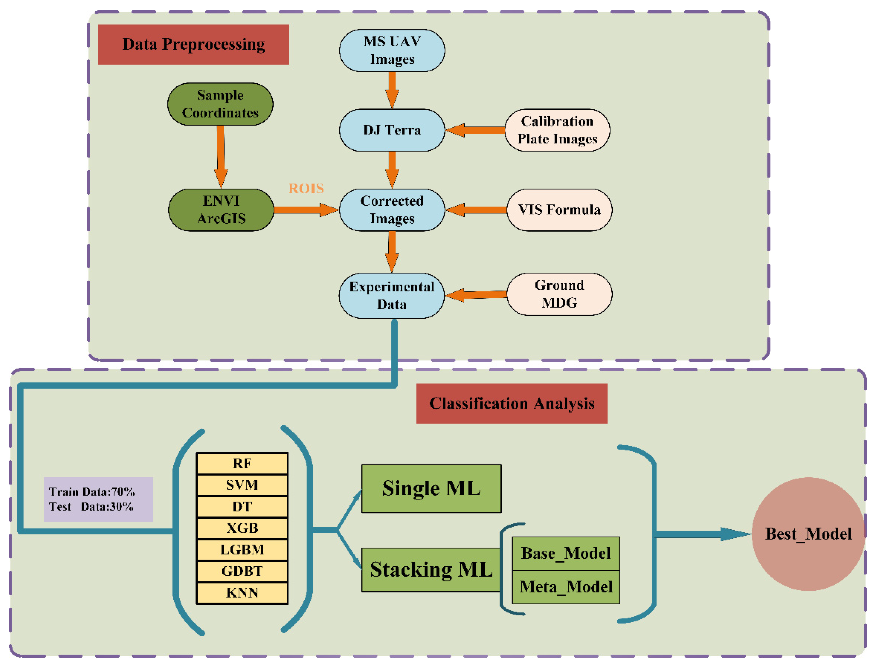
Multispectral UAV photos were input into DJI Terra v3.7.0 (DJI, Shenzhen, China), a UAV image stitching program optimized for DJI platforms. Calibration plate photos captured before each flight were also imported to perform radiometric calibration and ensure that the UAV images accurately represented surface reflectance. Because of the strong lighting conditions in Xinjiang, a calibration plate image was taken before each flight to maintain consistent stitching quality, and uniform lighting was selected for the reconstruction process. In farmland scenes, where smooth crop canopies can produce mirror-like reflection, this approach minimized brightness imbalance and improved image reconstruction quality. To ensure a coherent integration between UAV image acquisition and software processing, the entire workflow was designed as a continuous and reproducible process. Specifically, the multispectral UAV images collected using the Genie IV drone (DJI, Shenzhen, China) were first processed in DJI Terra for image stitching, radiometric calibration, and geometric correction to generate corrected single-band images. The corrected images were then imported into ArcGIS Pro v3.1 (Esri, Redlands, CA, USA) and ENVI v5.6.3 (L3Harris Geospatial, Broomfield, CO, USA), where the fixed ground sampling coordinates were used to define circular ROIs (radius 0.5 m). The mean reflectance of each ROI across the five spectral bands was calculated to form the experimental dataset. These reflectance values were then imported into Python v3.9.13 (Python Software Foundation, Wilmington, DE, USA) for vegetation index computation, feature normalization, and SHAP-based feature selection. This integrated procedure established a seamless link between UAV data acquisition, software preprocessing, and machine learning analysis, as summarized in Figure 4.
For reproducibility, the ROI of each sampling point was consistently defined as a circular area with a radius of 0.5 m centered on the fixed cotton plant. The mean reflectance R R O I for each spectral band was calculated using the following equation:
R R O I = 1 N i = 1 N R i
where R i is the reflectance of the i-th pixel in the ROI, and N is the total number of pixels. This procedure ensured consistent and reproducible extraction of spectral information for subsequent vegetation index calculations.

2.3. Construction and Selection of VIs

To identify the best vegetation index for assessing feasibility in the cotton boll stage, 52 vegetation indices were chosen based on prior research involving multispectral index computations; the corresponding calculation methods are provided in Table 3. Five individual multispectral bands that were radiometrically adjusted were used for all the vegetative indices. The primary inspiration for the SHAP value was from the Shapley value in cooperative game theory; Shapley proposed this variable in 1953 to gauge participants’ contributions and thus a procedure for allocating benefits [23]. In machine learning, SHAP values are used to quantify the eigenvalues of the contributions of inputs (importance) to the projected output [24]. The SHAP values of the model are computed in this study using SHAP-related Python tools [25].
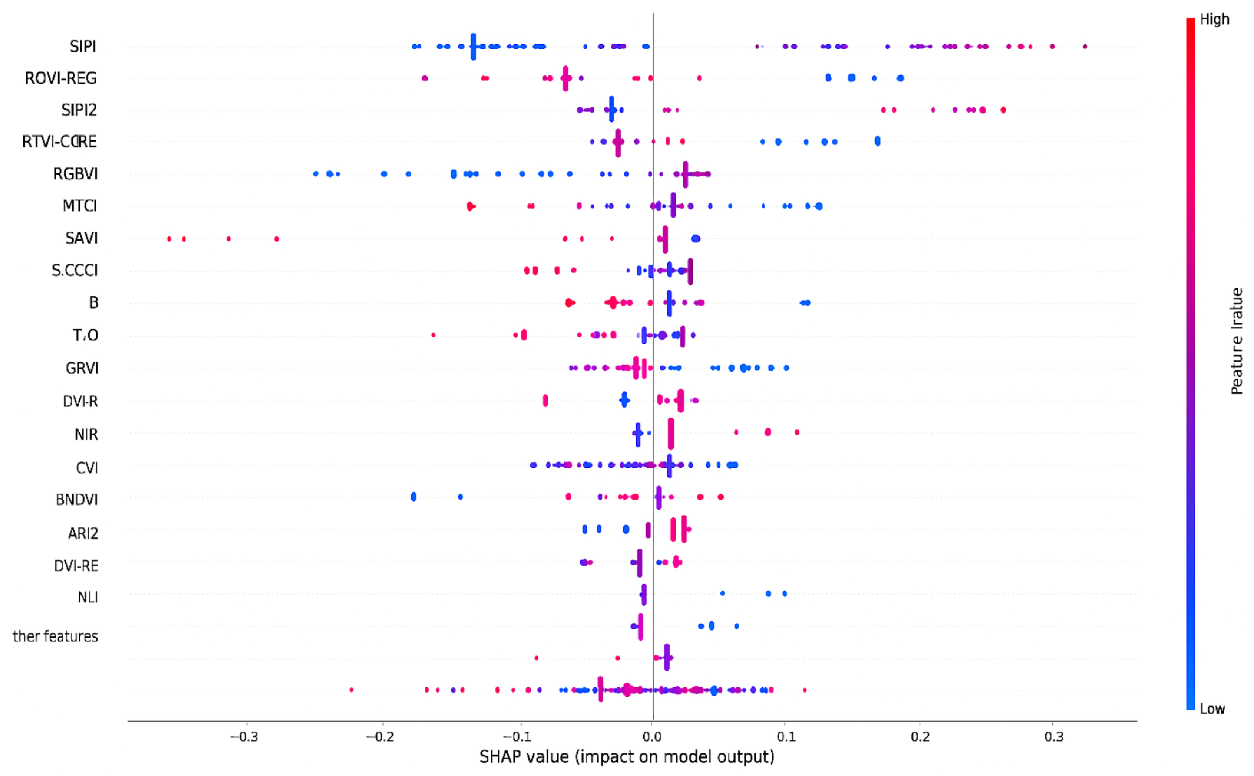
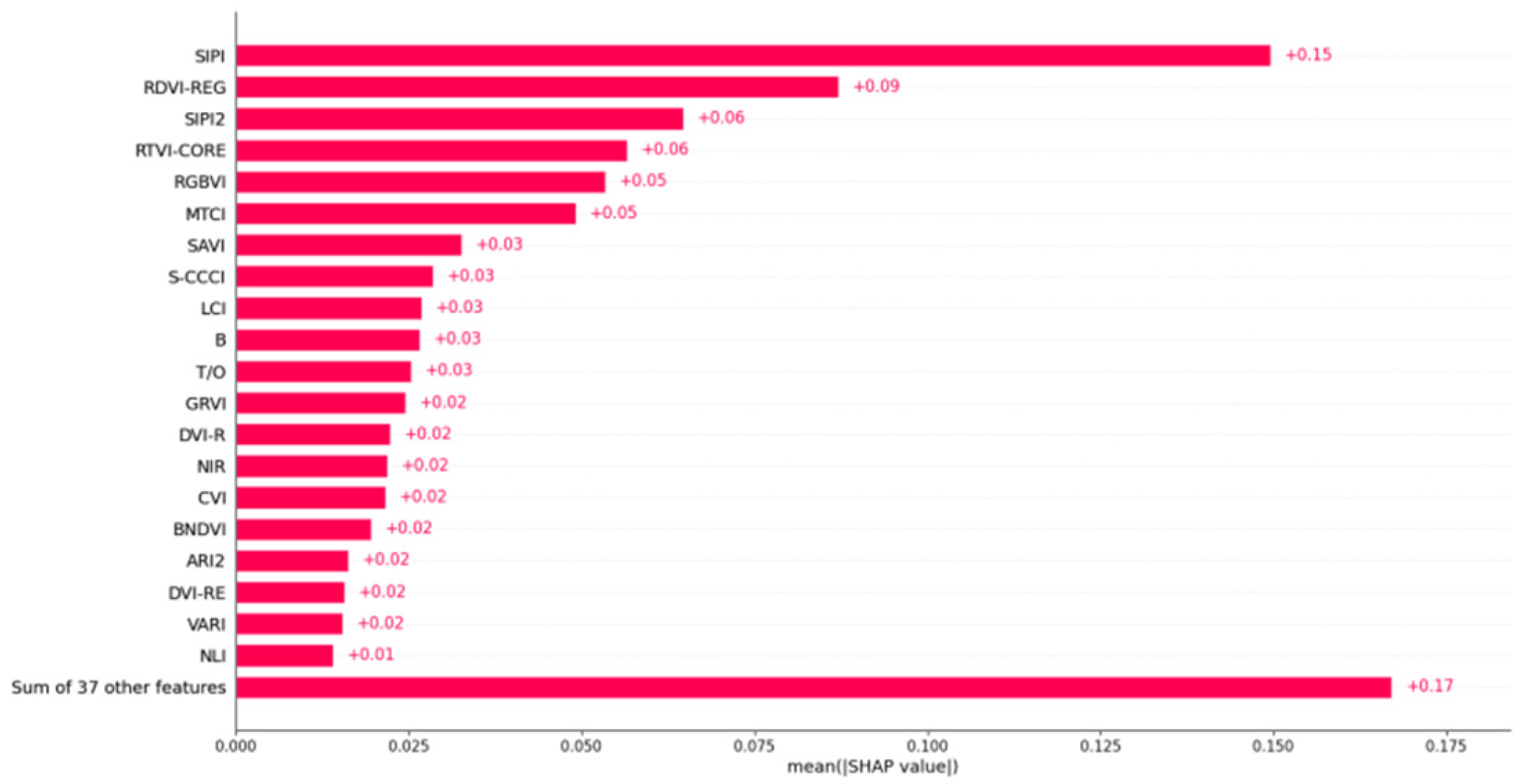
Figure 5 shows the distribution of various feature SHAP values across the entire sample. Each row in the figure represents a feature, and the horizontal coordinate is the SHAP value. The color denotes the effect of the magnitude of the feature value on the outcome, with the SHAP value or the weight of influence given on the horizontal axis, rather than the precise value of the feature (red indicates a large value, blue denotes a small value, and purple indicates values adjacent to the mean value). This graph is often wide at the top and narrow at the bottom because the larger the geographical distribution is, the greater the effect generally is (the influential factors are plotted at the top). It is clear that the model significantly benefits from the first six elements. The top N features that have the largest effects on the model are typically determined by averaging the absolute values of all features (abs()- > mean()); then, the absolute values are used to resolve positive and negative offsets and focus on the strength of the correlation. The results are given in Figure 5 without any statistical analysis. To determine the relative relevance of each variable to the model, we added the positive and negative impacts of each feature on the model. Consequently, unique SHAP values were obtained (Figure 6). Figure 6 shows that the first six SHAP values are considerably higher than the later SHAP values, as also supported by the results of the weighting analysis in Figure 5. Therefore, the first 6 features were chosen as model variables for further analysis.

2.4. Method

2.4.1. Classifier Model

Seven machine learning algorithms—Random Forest (RF), Support Vector Machine (SVM), Extreme Gradient Boosting (XGB), Light Gradient Boosting Machine (LGBM), K-Nearest Neighbors (KNN), Decision Tree (DT), and Gradient Boosting Decision Tree (GBDT)—were selected for comparison in this study. These models represent different learning paradigms (ensemble, kernel-based, instance-based, and tree-based approaches) and have been widely applied in UAV-based crop pest and disease classification tasks. The top-performing four models (XGB, GBDT, KNN, and DT) were later integrated into the stacking framework following the principle of model heterogeneity to enhance robustness and generalization. These traditional classification methods were used to build models for determining the levels of cotton leaf mite damage. For each approach, 10-fold cross-validation was used to increase generalizability and robustness, and GridSearchCV in the sklearn package of Python was used to optimize the hyperparameter search process. Permuting the potential values of each parameter and displaying all possible combinations result in a ‘grid’ during the grid search procedure. The models are then trained using the combinations of results, and cross-validation is performed to assess performance. The fitting function returns an appropriate classifier that automatically adapts to the optimal parameter combination after exploring all possible combinations of parameters. A grid search may take more time and require more computer memory resources than Bayesian optimization and random searches when determining the best optimization parameters, but locally optimal solutions are avoided, and the best parameters for the seven base classifiers considered in this study can be obtained. The ideal parameter values and the ideal search ranges for all parameters are listed in Table 4.

2.4.2. Stacking Model

Integrated learning is a machine learning paradigm, and stacking is a technique for integrated learning. In integrated learning, many models—often referred to as “weak learners”—are trained to address the same issue; then, these models are integrated to provide superior outcomes to those of individual models. Stacking is a machine learning approach based on integrated learning. The stacking approach provides a framework for hierarchical model integration, as shown in Figure 7. The initial data set is split into training and testing sets at a ratio of 70% to 30%. In this study, 10-fold cross-validation is employed. The training set is split into 10 points, and during each split, nine copies of the training set are made, with the remaining set used as the validation set. The validation set is used to obtain predictions with the model trained using the training set. The model obtained after training is also used for prediction, and predictions are compared to the values in the test set. The ten predictions for the validation set are then stitched together as the input values for the next stage of training, and the ten prediction outputs for the test set are averaged to create a new test set. The secondary learner is trained using the new training set and test set data. Overfitting is avoided to some extent because the training data varied and the resilience and generalizability of the model were enhanced.
It is noteworthy that the number of samples corresponding to different mite infestation levels was uneven, with a higher frequency of level 1 samples. To reduce the potential impact of class imbalance, 10-fold cross-validation and a stacked ensemble strategy were adopted to enhance the robustness and generalization of the model without introducing synthetic data, which is particularly important when the total number of samples is limited.

2.4.3. Accuracy Evaluation

Results of the evaluation experiment were assessed with standard multiclass evaluation indices, namely, accuracy, precision, recall, and F1-score, as this study involves a three-class problem. Specifically, these indices were used to thoroughly evaluate the stacking model for identifying and classifying cotton leaf mite infestation. In classification tasks, the F1-score is a popular assessment measure for evaluating the accuracy and recall of a model. The arithmetic mean values of the accuracy, recall, and F1-score for various categories are known as the macroaverages (Macro Avg). The overall performance of a classification model is frequently assessed using macroaveraging for various data sets. In a variation in macroaveraging known as weighted averaging (Weighted Avg), the proportion of samples from each category in the entire sample is considered when calculating the overall assessment indices.
The accuracy, macroaverage, and weighted average calculations are as follows:
A c c u r a c y = 1 k i = 1 k y i
P r e c i s i o n M a c r o   A v g = 1 k i = 1 k P i
P r e c i s i o n W e i g h t e d   A v g = i = 1 k P i   W i
The recall rate and F1 value formulas are the same as those for Macro Avg and Weighted Avg, where i is set as 1, 2, or 3 and Pi is the check rate (Precision) for cotton leaf mite damage at the levels considered in this study. Wi is the percentage of leaf mites associated with each class of damage.

3. Results

3.1. Single-Model Classification Results

The classification results of each individual model for the classification of leaf mites were obtained after hyperparameter optimization for each individual model based on a grid search process (see Table 4). As shown in Table 5, the accuracy of the seven base classification models, from high to low, was XGB: 0.825, GBDT: 0.810, KNN: 0.794, DT: 0.794, RF: 0.778, SVM: 0.762, and LGBM: 0.773. The most accurate model among the seven was XGB, and it consistently performed well in both macroaveraging and the weighted averaging. Comparatively, the DT and KNN algorithms yielded low accuracy in the case of macroaverage, mostly because more samples have a mite damage level of 1 than other damage levels, leading to skewed information gain in favor of more abundant features. Because of the wide region covered in aerial monitoring with the UAV and the high dependence on leaf surveys when confirming cotton leaf mite damage, in practice, some samples were likely labeled as class 1 mite infection that were not actually class 1. However, this inaccuracy was within the permitted limit of variation during classification.

3.2. Stacking and Integration of Individual Base Models

In general, the most robust and accurate classifiers are selected as the base model, which is the first layer of the stacked model, and less complex classifiers are typically used in the second layer. In the stacking process, the four most accurate single models (XGB, GBDT, KNN, and DT) were used as potential base and meta learners. Additionally, as shown in Table 6, we used a straightforward logistic linear regression (LLR) approach for the metamodel to provide different training effects, as described in prior research.
In the table, the results of the stacked models with single base models do not meet the relevant accuracy requirements. In these cases, the accuracy of the stacked models could not be increased with the LLR-based metamodel. This finding suggests that the stacked models developed in this study based on a single base model cannot satisfy the relevant classification accuracy requirements. However, it is also clear from the table that for the XGB, DT, and KNN models, the accuracy does not improve; additionally, the GBDT model performs poorly, with worse results than those of the single classification models. Thus, cases in which two, three, and four base models are stacked were explored to generate an effective model.

3.3. Stacked Integration of Two Base Models

Each classification evaluation index for the stacked models with two base models is greatly enhanced when DT and KNN metamodels are used. Additionally, XGB and KNN base models and DT and KNN metamodels yield the same results; these classification results are 6.7% more accurate than those of the individual XGB model, and the accuracy of the combined GBDT and KNN approach is 6.3% higher than that of the XGB model. The average accuracy is increased by 4.9% when the DT and KNN models are used together. Together with the single base model classification results in Table 6, these results suggest that the number of base models should be increased to improve model performance; still, no metamodels greatly improved the modeling effect. The precision of models that include a GBDT metamodel is comparatively low. Therefore, models using KNN or DT as the metamodel achieved relatively higher precision and overall stability, while those incorporating GBDT as the metamodel performed less effectively. These findings indicate that increasing the diversity and number of base models can further enhance the performance of the stacked framework, as discussed in the following section.

3.4. Stacked Integration of Multiple Base Models

In Table 7, the accuracy of the stacked integrated models with more than two base models remains the same and does not increase, indicating that increasing the number of base models will not necessarily produce better results in stacked learning and that only the right mix of base models and metamodels can be used to create a more effective integrated model. The accuracy of the stacked model with an LR metamodel increases with the number of base models, which may be because LR can lead to overfitting. The accuracy of the stacked models built with two base models among the XGB, GDBT, KNN, and DT models, as shown in Table 8, is consistent with the accuracy of the stacked models built with more base models in previous studies. For the case of this specific data set, the inclusion of extra base models beyond two provided no extra boost to accuracy.

3.5. Confusion Matrix Analysis

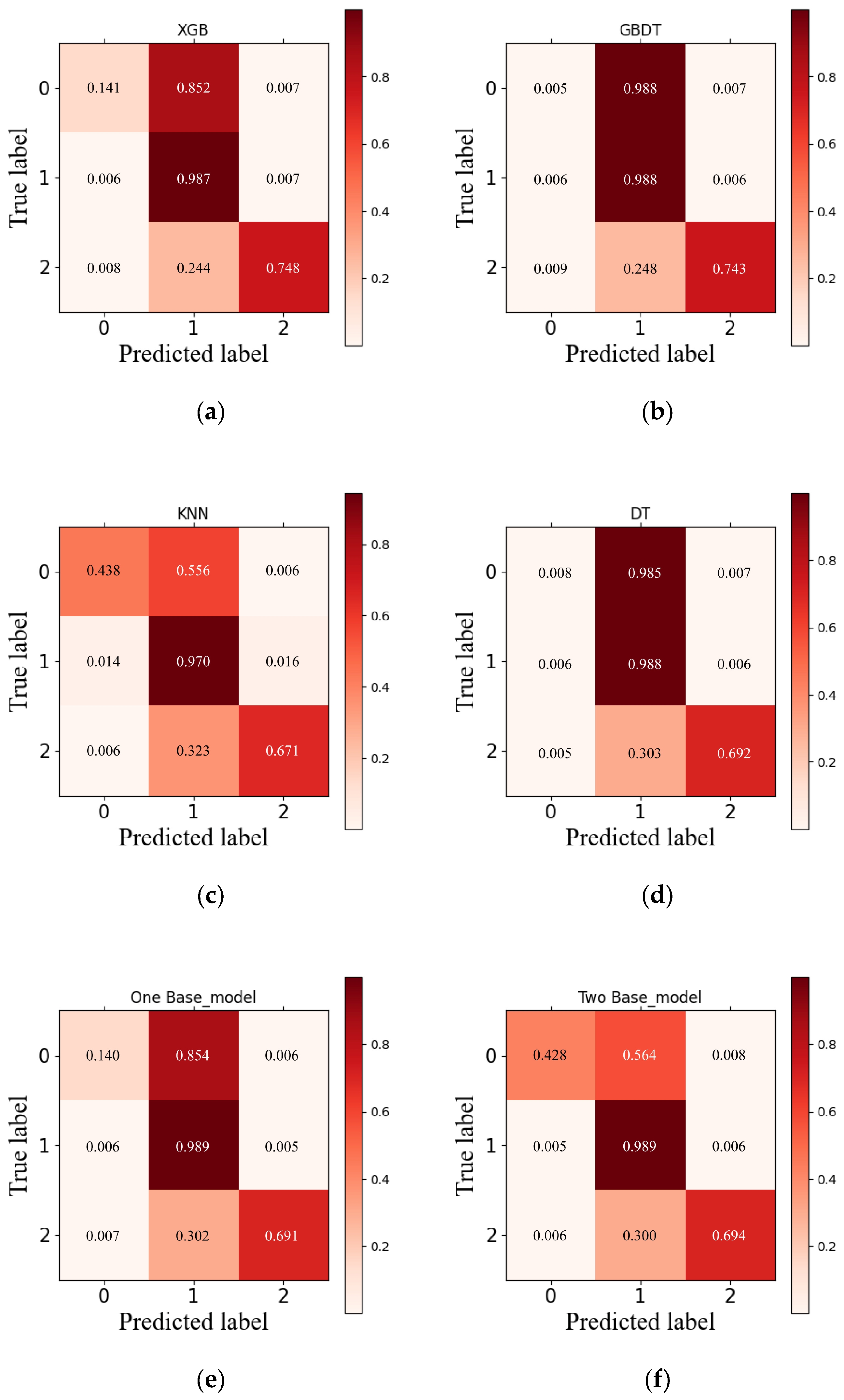
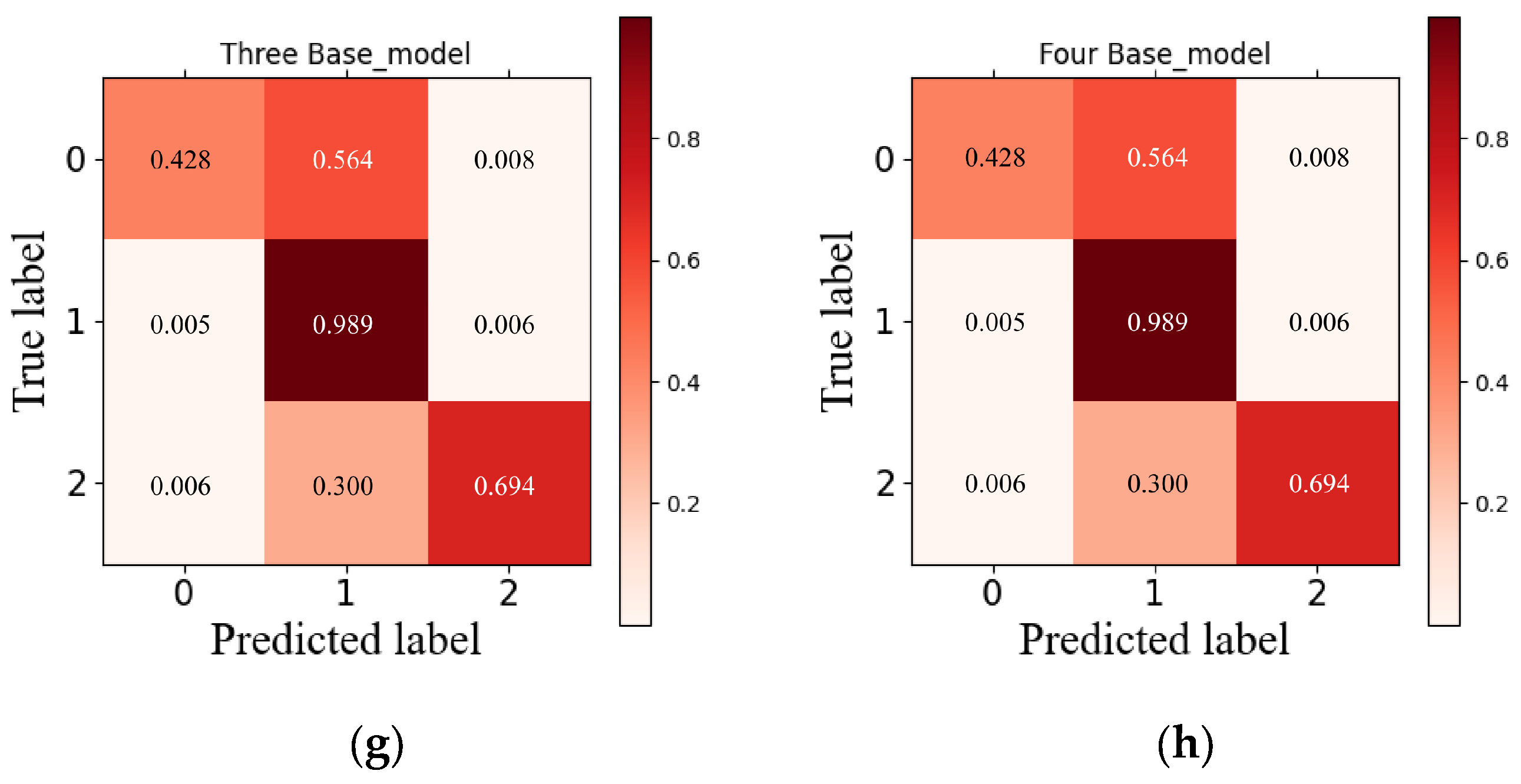
These confusion matrices (Figure 8) provide a clear visual interpretation of the classification performance, allowing direct comparison between the predicted and actual infestation levels. The diagonal line between X and Y roughly depicts the correlation between the actual and expected values. The x-axis represents the predicted outcomes, and the y-axis shows the actual values. The diagonal colors of the single GBDT and DT models in Figure 8b,d display differences and the differences remain consistent, indicating that some of the actual values for mite class 0 are predicted to be 1; additionally, the shades of the diagonal colors in Figure 8a,c show that the single XGB and KNN models are robust in the overall classification process. These models are more biased toward large samples with class 1 mites due to the limited number of samples for mite class 0. However, based on the overall classification accuracy of the GBDT and DT models in Table 5, these two single classification models still performed well overall. The classification of dangerous leaf mites, such as cotton leaf mites in classes 1 and 2, was highly accurate.
The confusion matrices in Figure 8e–h display higher accuracy and robustness than those for the single classification models, and the misclassification of level 0 mites as level 1 mites is mitigated. Figure 8e shows the result for a stacked model constructed from a single base model, and the accuracy and robustness of this model are lower than those of the single classification models. As shown in Figure 8, the most common off-diagonal misclassifications occur between level 0 and level 1 samples. In contrast, level 1 shows the highest classification accuracy among all classes, demonstrating the robustness of the proposed model. The stacked models with XGB and KNN base models and DT metamodels are the best performers in this study; however, increasing the number of models does not necessarily result in better results, particularly because computational memory use and resource use increase.

3.6. Visualization of Detection Results

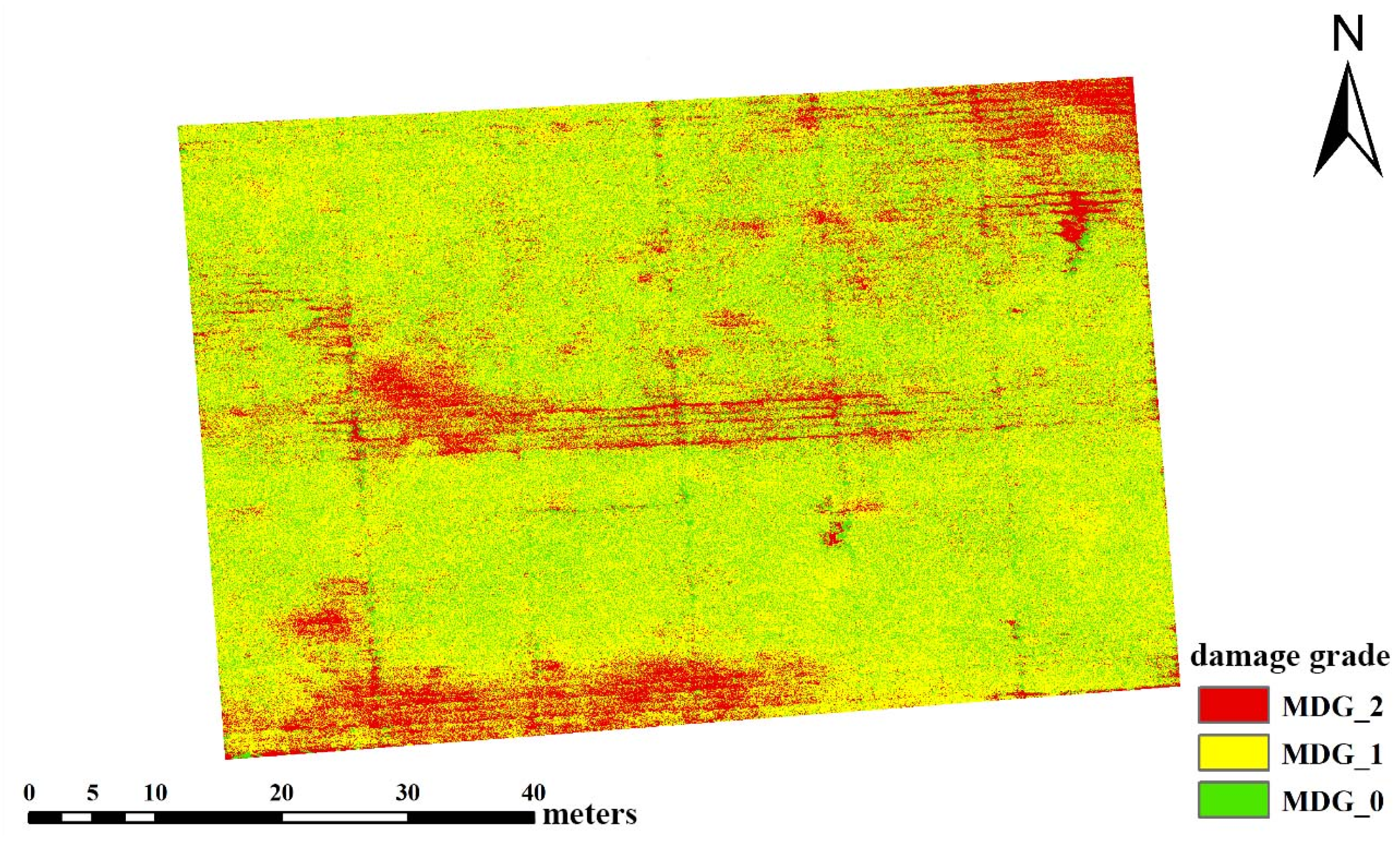
To further visually demonstrate the effectiveness of the optimal stacked model in detecting cotton leaf mite damage, the spatial distribution of the predicted infestation levels (MDG_0–MDG_2) was mapped using UAV multispectral data. As shown in Figure 9, The figure clearly demonstrates the model’s ability to identify and distinguish different degrees of mite damage across the study area, further confirming its effectiveness for UAV-based field-scale monitoring.

4. Discussion

4.1. Selection of the Optimal Base Model and Accuracy Evaluation

The most crucial factor in infestation analysis is not to identify a specific result for a certain crop but to build models with high generalizability and resilience in different detection cases. The selection of the base model is performed with the goal of creating classification models with broad applicability in different disciplines. The boosting algorithms considered were the XGB, GBDT, and LGBM algorithms; each weak learner is characterized by strong correlation dependence, and the weights of the subsequent learners are adjusted in accordance with the outcomes of the previous learners. For most data sets, boosting is more accurate than bagging, and the RF algorithm is a type of bagging algorithm.
Table 5 shows that the RF yields a lower accuracy than the boosting models, which is consistent with the outcomes of other experiments. For example, a similar result was obtained in an investigation of tomato pest diagnosis techniques based on data overlays [71]. The accuracy of single base models is typically lower than that of integrated algorithms when the DT, KNN, and SVM algorithms are used. However, an imbalance in sample data during classification and the bias in the DT and KNN methods may have resulted in higher accuracy for these methods in this study. Since the reflectance spectra of class 0 mite infestation and class 1 mite infestation are similar, it is likely that some of leaves were incorrectly classified, but the classification of class 0 as class 1 is within the allowable error range over the large monitored area. In this study, we extracted the average reflectance in the ROI of each sampling point as the spectral reflectance at that point.
When building stacked models, heterogeneity is frequently considered, and strong classifiers are chosen for the first layer while simpler classifiers are chosen for the second layer. For instance, when using integrated learning to estimate the maize LAI, a heterogeneous stacked integrated model with RF and MLR classifiers was used, and it achieved good results [72]. Although the RF and LGBM classifiers perform better than others in terms of macroaveraging and weighted averaging, they do not significantly increase the performance of the stacked models. Instead, the heterogeneous-based stacking models incorporate the advantages of each approach to provide a more complete model framework. The integrated XGB and GBDT models, which are boosting models, performed worse than the individual models, as seen in Table 6 and Table 8. This result further demonstrates that homogeneous stacking yields worse results than heterogeneous stacking. Therefore, the XGB, GDBT, KNN, and DT models were selected and integrated as base models in the stacked model.
The proposed stacked classification model, combining XGB and KNN as base learners and DT as the metamodel, achieved the highest performance, with an overall accuracy of 85.7% (macro-averaged F1-score: 78.2%; weighted-averaged F1-score: 84.7%). These results demonstrate that the model can effectively identify cotton leaf mite infestation levels using UAV multispectral imagery. Compared with previously published studies, the obtained accuracy is competitive or superior to most UAV- or machine-learning-based pest classification approaches. For example, Nguyen et al. [73] achieved monitoring accuracies of 60%, 71%, and 77% for early detection of wheat yellow rust at the tillering, heading, and flowering stages using multispectral UAV imagery combined with a 3D-CNN model. Cheney et al. [74] obtained an average identification accuracy of 83% for wheat canopy disease classification using hyperspectral reflectance derivatives with PLS and SVM models. Similarly, Aeberli et al. [75] reached a prediction accuracy of 86% for mite-infested banana plants using spectral feature selection and random forest classification. In contrast, the proposed stacking model integrates heterogeneous base learners (XGB, GBDT, KNN, and DT), which enhances robustness and adaptability under complex field conditions. This framework offers a well-balanced trade-off between accuracy and computational efficiency, making it highly suitable for practical and large-scale agricultural pest monitoring applications.

4.2. Discussion of Stacking Methods

There are three main stacking methods. The first one involves using a new training set obtained from the base model using cross-validation as the metamodel training set. The second method involves inputting the category probability values produced by all base classifiers in the first layer into the metamodel. To construct the training set for the metamodel, various features from several base models must be included, and a third parameter setting, namely, use_probas = True, is added to the StackingCVClassifier. Table 9 provides a comparison of the model findings for the second and third approaches. For the second method, the original spectral reflectance of the data is mapped to a probability interval based on the category probabilities created from the base model results, and this information is input into the metamodel. This approach may result in the loss of the characteristics of the original spectral reflectance, and the resulting model will be homogeneous in nature. The third construction method involves training with various features and base models to create new features for the metamodel in accordance with the distribution of SHAP values. However, in this study, the training results obtained with this approach were not as good as those for the ideal model, possibly because some features were not considered by certain base classifiers, which contributed to the poor overall performance of the integrated model.
The average mite damage level at 90 sampling points was examined in another cotton experimental plot to test the generalizability of the optimal proposed model. Figure 10 visually demonstrates the consistency between the predicted and observed infestation levels, confirming the effectiveness and reliability of the proposed stacking model. The overall accuracy was 82.2%, and the model may have been affected by human error in the manual surveys conducted at different times. The average mite damage level was incorrectly predicted at 16 sample locations. Although the validation dataset included only 90 points, these samples were collected from a plot with environmental and management conditions distinct from those used for model training. Therefore, the results provide preliminary evidence that the trained model can achieve satisfactory classification performance under different field conditions. Nevertheless, we acknowledge that a more extensive validation using multi-season and multi-location datasets is necessary to further confirm the model’s generalization ability, which will be the focus of future work.

4.3. Practical Usability and Runtime Analysis

To further evaluate the practical usability of the proposed stacking model, a runtime analysis was performed to measure both the training and inference efficiency. The experiments were conducted on a workstation equipped with an Intel Core i7-12700 CPU, 32 GB RAM, and an NVIDIA RTX 3060 GPU. The average inference time per image for the stacking model was approximately 0.18 s, which is only slightly higher than that of the single XGB model (0.14 s). This finding indicates that, although the stacked architecture introduces an additional computational layer, it still maintains acceptable efficiency for UAV-based near real-time monitoring applications. The training process of the stacking model required approximately 1.35 times the training time of a single model, mainly due to cross-validation and the combination of base learners. Nevertheless, the improvement in classification accuracy and robustness justifies this computational overhead. Overall, the runtime performance suggests that the proposed stacking model achieves a reasonable balance between accuracy and efficiency. In future work, model compression, pruning, and lightweight ensemble techniques will be explored to further reduce inference time while maintaining high accuracy.

4.4. Limitations of the Research

(1) Under high-temperature and extreme drought conditions, cotton leaf mites often move from the bottom to the top of the lowest leaves. As a result, water stress is likely to occur in areas where cotton leaf mites are severe, which is a concern for further research. Further studies employing penetrating LiDAR, or similar methods, can be performed in the future to explore dense cotton canopies and assess the ability of UAVs to monitor cotton leaf mite damage below the canopy.
(2) Although the proposed method achieved satisfactory performance in classifying cotton leaf mite infestation levels, certain limitations should be acknowledged. The dataset used in this study comprised only 90 sampling points, resulting in a relatively small number of samples for both training and testing. Such a limited sample size may restrict the representativeness of the dataset and introduce uncertainty in the estimation of model accuracy, leading to broader confidence intervals. Moreover, the class distribution of the dataset was imbalanced, with level 1 mite damage samples being predominant. This imbalance may have biased the learning process of individual classifiers. Although the number of ground survey samples was limited (n = 90), a 10-fold cross-validation and independent test evaluation were applied to reduce potential overfitting. To alleviate potential overfitting and mitigate the effects of data imbalance, a 10-fold cross-validation strategy and a stacked ensemble framework were adopted, which diversified the training subsets and enhanced model robustness. Nevertheless, the influence of imbalance on classification performance cannot be entirely ruled out. Future studies should consider expanding the sampling area, increasing the number of field samples, and employing class-balancing techniques such as SMOTE or cost-sensitive learning to further validate and strengthen the model’s generalizability.
(3) In this study, classes 0 (“No harm”) and 1 (“sporadic white dots”) were merged due to the difficulty of distinguishing them in UAV-based monitoring at low altitudes. While this simplification improves the robustness of classification under practical field conditions, it inevitably limits the model’s sensitivity to extremely early-stage infestations—precisely the stage when intervention is most efficient and cost-effective. Future work should focus on developing higher-resolution UAV imaging or hyperspectral sensing techniques to separate these subtle classes more accurately and enable earlier detection for more effective pest management.

5. Conclusions

This study developed a UAV multispectral image-based model for classifying cotton leaf mite infestation severity. By integrating SHAP value theory to screen key vegetation indices and combining multiple machine learning algorithms through a stacked ensemble framework, the proposed method effectively reduces feature redundancy and enhances model interpretability. Among the tested configurations, the stacked models constructed with XGB, KNN, and DT base learners achieved the highest classification accuracy and robustness, demonstrating superior performance over individual machine learning models. Compared with existing studies that mainly focus on binary pest detection, this research establishes a more refined and interpretable approach capable of distinguishing multiple infestation levels. The combination of SHAP-based feature selection and heterogeneous stacking enhances accuracy, generalization, and computational efficiency, providing a reliable foundation for UAV-based pest and disease monitoring in precision agriculture. Although the limited number of ground survey samples (n = 90) may introduce potential overfitting risks, 10-fold cross-validation and independent testing were employed to ensure model reliability. Future work will expand the dataset, explore temporal UAV imagery, and further optimize the ensemble structure to improve generalization. The proposed framework also holds promise for broader applications in UAV-assisted monitoring of other crop pests and diseases, contributing to data-driven sustainable crop management.

Author Contributions

Conceptualization, S.F.; methodology, S.F. and W.G.; software, Y.C.; validation, X.X. and W.G.; formal analysis, X.X.; investigation, Q.H.; resources, Y.L.; data curation, Q.H.; writing—original draft preparation, S.F.; writing—review and editing, H.Q.; visualization, Y.C. and X.X.; supervision, H.Q.; project administration, Y.L. and J.L.; funding acquisition, Y.L., J.L. and H.Q. All authors have read and agreed to the published version of the manuscript.

Funding

This study was funded by Key R&D projects during the 14th Five Year Plan period [2022YFD1400302] and the National Natural Science Foundation of China [U2003119].

Data Availability Statement

The data presented in this study are available on request from the corresponding author due to the data also form part of an ongoing study.

Conflicts of Interest

The authors declare no conflicts of interest.

References

  1. Li, Y.; Yang, J. Few-shot cotton pest recognition and terminal realization. Comput. Electron. Agric. 2020, 169, 105240. [Google Scholar] [CrossRef]
  2. Xu, W.; Yang, W.; Chen, S.; Wu, C.; Chen, P.; Lan, Y. Establishing a model to predict the single boll weight of cotton in northern Xinjiang by using high resolution UAV remote sensing data. Comput. Electron. Agric. 2020, 179, 105762. [Google Scholar] [CrossRef]
  3. He, L.; Shi, L.; Liu, G.; Liang, C.T. Occurrence and control of pests and diseases in the Northwest Inland Cotton Area of China. Phytoparasitica 2025, 53, 81. [Google Scholar] [CrossRef]
  4. Zhu, H.; Lin, C.; Liu, G.; Wang, D.; Qin, S.; Li, A.; Xu, J.L.; He, Y. Intelligent agriculture: Deep learning in UAV-based remote sensing imagery for crop diseases and pests detection. Front. Plant Sci. 2024, 15, 1435016. [Google Scholar] [CrossRef] [PubMed]
  5. Zhang, S.; Li, X.; Ba, Y.; Lyu, X.; Zhang, M.; Li, M. Banana Fusarium Wilt Disease Detection by Supervised and Unsupervised Methods from UAV-Based Multispectral Imagery. Remote Sens. 2022, 14, 1231. [Google Scholar] [CrossRef]
  6. Chen, P.; Xu, W.; Zhan, Y.; Wang, G.; Yang, W.; Lan, Y. Determining application volume of unmanned aerial spraying systems for cotton defoliation using remote sensing images. Comput. Electron. Agric. 2022, 196, 106912. [Google Scholar] [CrossRef]
  7. Yang, W.; Xu, W.; Wu, C.; Zhu, B.; Chen, P.; Zhang, L.; Lan, Y. Cotton hail disaster classification based on drone multispectral images at the flowering and boll stage. Comput. Electron. Agric. 2021, 180, 105866. [Google Scholar] [CrossRef]
  8. Huang, H.; Deng, J.; Lan, Y.; Yang, A.; Deng, X.; Zhang, L.; Wen, S.; Jiang, Y.; Suo, G.; Chen, P. A two-stage classification approach for the detection of spider mite- infested cotton using UAV multispectral imagery. Remote Sens. Lett. 2018, 9, 933–941. [Google Scholar] [CrossRef]
  9. Ren, C.N.; Liu, B.; Liang, Z.; Lin, Z.L.; Wang, W.; Wei, X.Z.; Li, X.J.; Zou, X.J. An Innovative Method of Monitoring Cotton Aphid Infestation Based on Data Fusion and Multi-Source Remote Sensing Using Unmanned Aerial Vehicles. Drones 2025, 9, 229. [Google Scholar] [CrossRef]
  10. Sun, C.L.; Bin, A.A.; Wang, Z.Y.; Gao, X.X.; Ding, K. YOLO-UP: A High-Throughput Pest Detection Model for Dense Cotton Crops Utilizing UAV-Captured Visible Light Imagery. IEEE Access 2025, 13, 19937–19945. [Google Scholar] [CrossRef]
  11. Ali, T.; Zakir, R.; Ayaz, M.; Murtaza, M.; Hijji, M.; Aggoune, E.M.H. Cotton crop disease detection and classification using statistical prediction model in deep learning approach. Multimed. Tools Appl. 2025. [Google Scholar] [CrossRef]
  12. Alves, A.N.; Souza, W.S.R.; Borges, D.L. Cotton pests classification in field-based images using deep residual networks. Comput. Electron. Agric. 2020, 174, 105488. [Google Scholar] [CrossRef]
  13. Zheng, Z.J.; Yuan, J.H.; Yao, W.; Kwan, P.; Yao, H.X.; Liu, Q.Z.; Guo, L.F. Fusion of UAV-Acquired Visible Images and Multispectral Data by Applying Machine-Learning Methods in Crop Classification. Agronomy 2024, 14, 2670. [Google Scholar] [CrossRef]
  14. Pandiyaraju, v.; Anusha, B.; Senthil Kumar, A.M.; Jaspin, K.; Venkatraman, S.; Kannan, A. Spatial attention-based hybrid VGG-SVM and VGG-RF frameworks for improved cotton leaf disease detection. Neural Comput. Appl. 2025, 37, 8309–8329. [Google Scholar] [CrossRef]
  15. Qiu, Z.; Ma, F.; Li, Z.; Xu, X.; Ge, H.; Du, C. Estimation of nitrogen nutrition index in rice from UAV RGB images coupled with machine learning algorithms. Comput. Electron. Agric. 2021, 189, 106421. [Google Scholar] [CrossRef]
  16. Healey, S.P.; Cohen, W.B.; Yang, Z.; Kenneth Brewer, C.; Brooks, E.B.; Gorelick, N.; Hernandez, A.J.; Huang, C.; Joseph Hughes, M.; Kennedy, R.E.; et al. Mapping forest change using stacked generalization: An ensemble approach. Remote Sens. Environ. 2018, 204, 717–728. [Google Scholar] [CrossRef]
  17. Xiao, Y.; Guo, Y.; Yin, G.; Zhang, X.; Shi, Y.; Hao, F.; Fu, Y. UAV Multispectral Image-Based Urban River Water Quality Monitoring Using Stacked Ensemble Machine Learning Algorithms—A Case Study of the Zhanghe River, China. Remote Sens. 2022, 14, 3272. [Google Scholar] [CrossRef]
  18. Fu, B.; He, X.; Yao, H.; Liang, Y.; Deng, T.; He, H.; Fan, D.; Lan, G.; He, W. Comparison of RFE-DL and stacking ensemble learning algorithms for classifying mangrove species on UAV multispectral images. Int. J. Appl. Earth Obs. Geoinf. 2022, 112, 102890. [Google Scholar] [CrossRef]
  19. Yang, M.D.; Hsu, Y.C.; Chen, Y.H.; Yang, C.Y.; Li, K.Y. Precision monitoring of rice nitrogen fertilizer levels based on machine learning and UAV multispectral imagery. Comput. Electron. Agric. 2025, 237, 110523. [Google Scholar] [CrossRef]
  20. Deng, L.Q.; Li, Y.Y.; Zhang, Z.M.; Mu, J.J.; Jia, S.J.; Yan, Y.Q.; Zhang, W.P. Sorghum yield prediction using UAV multispectral imaging and stacking ensemble learning in arid regions. Front. Plant Sci. 2025, 16, 1636015. [Google Scholar] [CrossRef]
  21. Du, R.Q.; Lu, J.S.; Xiang, Y.Z.; Zhang, F.C.; Chen, J.Y.; Tang, Z.J.; Shi, H.Z.; Wang, X.; Li, W.Y. Estimation of winter canola growth parameter from UAV multi-angular spectral-texture information using stacking-based ensemble learning model. Comput. Electron. Agric. 2024, 222, 109074. [Google Scholar] [CrossRef]
  22. GB/T 15802-2011; Technical Specification for Cotton Leaf Mite Detection and Reporting. Domestic—National Standards—State Administration of Market Supervision and Administration CN-GB: Beijing, China, 2011.
  23. Shapley, L.S. A value for n-person games. Class. Game Theory 1997, 69–79. [Google Scholar] [CrossRef]
  24. Wang, J.; Wiens, J.; Lundberg, S.M. Shapley Flow: A Graph-based Approach to Interpreting Model Predictions. Int. Conf. Artif. Intell. Stat. 2021, 130, 721–729. [Google Scholar]
  25. Lundberg, S.M.; Erion, G.; Chen, H.; DeGrave, A.; Prutkin, J.M.; Nair, B.; Katz, R.; Himmelfarb, J.; Bansal, N.; Lee, S.I. From Local Explanations to Global Understanding with Explainable AI for Trees. Nat. Mach. Intell. 2020, 2, 56–67. [Google Scholar] [CrossRef]
  26. Wang, F.; Yang, M.; Ma, L.; Zhang, T.; Qin, W.; Li, W.; Zhang, Y.; Sun, Z.; Wang, Z.; Li, F.; et al. Estimation of Above-Ground Biomass of Winter Wheat Based on Consumer-Grade Multi-Spectral UAV. Remote Sens. 2022, 14, 1251. [Google Scholar] [CrossRef]
  27. Gitelson, A.A.; Gritz, Y.; Merzlyak, M.N. Relationships between leaf chlorophyll content and spectral reflectance and algorithms for non-destructive chlorophyll assessment in higher plant leaves. J. Plant Physiol. 2003, 160, 271–282. [Google Scholar] [CrossRef]
  28. Qi, H.; Wu, Z.; Zhang, L.; Li, J.; Zhou, J.; Jun, Z.; Zhu, B. Monitoring of peanut leaves chlorophyll content based on drone-based multispectral image feature extraction. Comput. Electron. Agric. 2021, 187, 106292. [Google Scholar] [CrossRef]
  29. Xiao, Y.; Zhao, W.; Zhou, D.; Gong, H. Sensitivity Analysis of Vegetation Reflectance to Biochemical and Biophysical Variables at Leaf, Canopy, and Regional Scales. IEEE Trans. Geosci. Remote Sens. 2014, 52, 4014–4024. [Google Scholar] [CrossRef]
  30. Haboudane, D. Hyperspectral vegetation indices and novel algorithms for predicting green LAI of crop canopies: Modeling and validation in the context of precision agriculture. Remote Sens. Environ. 2004, 90, 337–352. [Google Scholar] [CrossRef]
  31. Gitelson, A.A.; Kaufman, Y.J.; Stark, R.; Rundquist, D. Novel algorithms for remote estimation of vegetation fraction. Remote Sens. Environ. 2002, 80, 76–87. [Google Scholar] [CrossRef]
  32. Ji, Y.; Chen, Z.; Cheng, Q.; Liu, R.; Li, M.; Yan, X.; Li, G.; Wang, D.; Fu, L.; Ma, Y.; et al. Estimation of plant height and yield based on UAV imagery in faba bean (Vicia faba L.). Plant Methods 2022, 18, 26. [Google Scholar] [CrossRef] [PubMed]
  33. Huete, A. A soil-adjusted vegetation index (SAVI). Remote Sens. Environ. 1988, 25, 295–309. [Google Scholar] [CrossRef]
  34. Zhen, Z.J.; Chen, S.B.; Yin, T.G.; Chavanon, E.; Lauret, N.; Guilleux, J.; Henke, M.; Qin, W.H.; Cao, L.S.; Li, J.; et al. the Negative Soil Adjustment Factor of Soil Adjusted Vegetation Index (SAVI) to Resist Saturation Effects and Estimate Leaf Area Index (LAI) in Dense Vegetation Areas. Sensors 2021, 21, 2115. [Google Scholar] [CrossRef] [PubMed]
  35. Ren, H.R.; Zhou, G.S.; Zhang, F. Using negative soil adjustment factor in soil-adjusted vegetation index (SAVI) for aboveground living biomass estimation in arid grasslands. Remote Sens. Environ. 2018, 209, 439–445. [Google Scholar] [CrossRef]
  36. Roujean, J.-L.; Breon, F.-M. Estimating PAR absorbed by vegetation from bidirectional reflectance measurements. Remote Sens. Environ. 1995, 51, 375–384. [Google Scholar] [CrossRef]
  37. Gitelson, A.A. Remote estimation of crop fractional vegetation cover: The use of noise equivalent as an indicator of performance of vegetation indices. Int. J. Remote Sens. 2013, 34, 6054–6066. [Google Scholar] [CrossRef]
  38. Bannari, A.; Asalhi, H.; Teillet, P.M. Transformed difference vegetation index (TDVI) for vegetation cover mapping. IEEE Int. Geosci. Remote Sens. Symp. 2002, 5, 3053–3055. [Google Scholar] [CrossRef]
  39. Jordan, C.F. Derivation of leaf-area index from quality of light on the forest floor. Ecology 1969, 50, 663–666. [Google Scholar] [CrossRef]
  40. Chen, J.M. Evaluation of Vegetation Indices and a Modified Simple Ratio for Boreal Applications. Can. J. Remote Sens. 2014, 22, 229–242. [Google Scholar] [CrossRef]
  41. Goel, N.S.; Qin, W. Influences of canopy architecture on relationships between various vegetation indices and LAI and Fpar: A computer simulation. Remote Sens. Rev. 1994, 10, 309–347. [Google Scholar] [CrossRef]
  42. Peng, G.; Ruiliang, P.; Biging, G.S.; Larrieu, M.R. Estimation of forest leaf area index using vegetation indices derived from hyperion hyperspectral data. IEEE Trans. Geosci. Remote Sens. 2003, 41, 1355–1362. [Google Scholar] [CrossRef]
  43. Su, J.; Yi, D.; Coombes, M.; Liu, C.; Zhai, X.; McDonald-Maier, K.; Chen, W.-H. Spectral analysis and mapping of blackgrass weed by leveraging machine learning and UAV multispectral imagery. Comput. Electron. Agric. 2022, 192, 106621. [Google Scholar] [CrossRef]
  44. Gitelson, A.A.; Merzlyak, M.N.; Chivkunova, O.B. Optical properties and nondestructive estimation of anthocyanin content in plant leaves. Photochem. Photobiol. 2001, 74, 38–45. [Google Scholar] [CrossRef] [PubMed]
  45. Gitelson, A.A.; Merzlyak, M.N.; Lichtenthaler, H.K. Detection of Red Edge Position and Chlorophyll Content by Reflectance Measurements Near 700 nm. J. Plant Physiol. 1996, 148, 501–508. [Google Scholar] [CrossRef]
  46. Siegmann, B.; Jarmer, T.; Lilienthal, H.; Richter, N.; Selige, T.; Höfled, B. Comparison of narrow band vegetation indices and empirical models from hyperspectral remote sensing data for the assessment of wheat nitrogen concentration. In Proceedings of the 8th EARSeL Workshop on Imaging Spectroscopy, Nantes, France, 8–10 April 2013; pp. 8–10. [Google Scholar]
  47. Hassan, M.; Yang, M.; Rasheed, A.; Jin, X.; Xia, X.; Xiao, Y.; He, Z. Time-Series Multispectral Indices from Unmanned Aerial Vehicle Imagery Reveal Senescence Rate in Bread Wheat. Remote Sens. 2018, 10, 809. [Google Scholar] [CrossRef]
  48. Wang, F.-m.; Huang, J.-f.; Tang, Y.-l.; Wang, X.-z. New Vegetation Index and Its Application in Estimating Leaf Area Index of Rice. Rice Sci. 2007, 14, 195–203. [Google Scholar] [CrossRef]
  49. Clevers, J.; Kooistra, L.; van den Brande, M. Using Sentinel-2 Data for Retrieving LAI and Leaf and Canopy Chlorophyll Content of a Potato Crop. Remote Sens. 2017, 9, 405. [Google Scholar] [CrossRef]
  50. Vincini, M.; Frazzi, E.; D’Alessio, P. A broad-band leaf chlorophyll vegetation index at the canopy scale. Precis. Agric. 2008, 9, 303–319. [Google Scholar] [CrossRef]
  51. Huete, A.; Didan, K.; Miura, T.; Rodriguez, E.P.; Gao, X.; Ferreira, L.G. Overview of the radiometric and biophysical performance of the MODIS vegetation indices. Remote Sens. Environ. 2002, 83, 195–213. [Google Scholar] [CrossRef]
  52. Jiang, Z.; Huete, A.; Didan, K.; Miura, T. Development of a two-band enhanced vegetation index without a blue band. Remote Sens. Environ. 2008, 112, 3833–3845. [Google Scholar] [CrossRef]
  53. Tucker, C.J. Red and photographic infrared linear combinations for monitoring vegetation. Remote Sens. Environ. 1979, 8, 127–150. [Google Scholar] [CrossRef]
  54. Daughtry, C.S.; Walthall, C.; Kim, M.; De Colstoun, E.B.; McMurtrey Iii, J. Estimating corn leaf chlorophyll concentration from leaf and canopy reflectance. Remote Sens. Environ. 2000, 74, 229–239. [Google Scholar] [CrossRef]
  55. García-Fernández, M.; Sanz-Ablanedo, E.; Rodríguez-Pérez, J.R. High-Resolution Drone-Acquired RGB Imagery to Estimate Spatial Grape Quality Variability. Agronomy 2021, 11, 655. [Google Scholar] [CrossRef]
  56. Dash, J.; Curran, P.J. The MERIS terrestrial chlorophyll index. Int. J. Remote Sens. 2010, 25, 5403–5413. [Google Scholar] [CrossRef]
  57. Gitelson, A.A.; Merzlyak, M.N. Remote estimation of chlorophyll content in higher plant leaves. Int. J. Remote Sens. 2010, 18, 2691–2697. [Google Scholar] [CrossRef]
  58. Agapiou, A.; Alexakis, D.D.; Stavrou, M.; Sarris, A.; Themistocleous, K.; Hadjimitsis, D.G. Prospects and limitations of vegetation indices in archeological research: The Neolithic Thessaly case study. Proc. SPIE Int. Soc. Opt. Eng. 2013, 8893, 969–970. [Google Scholar] [CrossRef]
  59. Parra, L.; Mostaza-Colado, D.; Marin, J.F.; Mauri, P.V.; Lloret, J. Methodology to Differentiate Legume Species in Intercropping Agroecosystems Based on UAV with RGB Camera. Electronics 2022, 11, 609. [Google Scholar] [CrossRef]
  60. Bendig, J.; Yu, K.; Aasen, H.; Bolten, A.; Bennertz, S.; Broscheit, J.; Gnyp, M.L.; Bareth, G. Combining UAV-based plant height from crop surface models, visible, and near infrared vegetation indices for biomass monitoring in barley. Int. J. Appl. Earth Obs. Geoinf. 2015, 39, 79–87. [Google Scholar] [CrossRef]
  61. Walsh, O.S.; Shafian, S.; Marshall, J.M.; Jackson, C.; McClintick-Chess, J.R.; Blanscet, S.M.; Swoboda, K.; Thompson, C.; Belmont, K.M.; Walsh, W.L. Assessment of UAV based vegetation indices for nitrogen concentration estimation in spring wheat. Adv. Remote Sens. 2018, 7, 71–90. [Google Scholar] [CrossRef]
  62. Verrelst, J.; Schaepman, M.E.; Koetz, B.; Kneubühler, M. Angular sensitivity analysis of vegetation indices derived from CHRIS/PROBA data. Remote Sens. Environ. 2008, 112, 2341–2353. [Google Scholar] [CrossRef]
  63. Raper, T.B.; Varco, J.J. Canopy-scale wavelength and vegetative index sensitivities to cotton growth parameters and nitrogen status. Precis. Agric. 2014, 16, 62–76. [Google Scholar] [CrossRef]
  64. Peñuelas, J.; Gamon, J.; Fredeen, A.; Merino, J.; Field, C. Reflectance indices associated with physiological changes in nitrogen-and water-limited sunflower leaves. Remote Sens. Environ. 1994, 48, 135–146. [Google Scholar] [CrossRef]
  65. Haboudane, D.; Miller, J.R.; Tremblay, N.; Zarco-Tejada, P.J.; Dextraze, L. Integrated narrow-band vegetation indices for prediction of crop chlorophyll content for application to precision agriculture. Remote Sens. Environ. 2002, 81, 416–426. [Google Scholar] [CrossRef]
  66. Broge, N.H.; Leblanc, E. Comparing prediction power and stability of broadband and hyperspectral vegetation indices for estimation of green leaf area index and canopy chlorophyll density. Remote Sens. Environ. 2001, 76, 156–172. [Google Scholar] [CrossRef]
  67. Velusamy, P.; Rajendran, S.; Mahendran, R.K.; Naseer, S.; Shafiq, M.; Choi, J.-G. Unmanned Aerial Vehicles (UAV) in Precision Agriculture: Applications and Challenges. Energies 2021, 15, 217. [Google Scholar] [CrossRef]
  68. Guo, A.; Huang, W.; Dong, Y.; Ye, H.; Ma, H.; Liu, B.; Wu, W.; Ren, Y.; Ruan, C.; Geng, Y. Wheat Yellow Rust Detection Using UAV-Based Hyperspectral Technology. Remote Sens. 2021, 13, 123. [Google Scholar] [CrossRef]
  69. Martin, D.E.; Latheef, M.A. Remote Sensing Evaluation of Two-spotted Spider Mite Damage on Greenhouse Cotton. J. Vis. Exp. 2017, 122, 54314. [Google Scholar] [CrossRef]
  70. Reid, A.M.; Chapman, W.K.; Prescott, C.E.; Nijland, W. Using excess greenness and green chromatic coordinate colour indices from aerial images to assess lodgepole pine vigour, mortality and disease occurrence. For. Ecol. Manag. 2016, 374, 146–153. [Google Scholar] [CrossRef]
  71. Xu, C.; Ding, J.; Qiao, Y.; Zhang, L. Tomato disease and pest diagnosis method based on the Stacking of prescription data. Comput. Electron. Agric. 2022, 197, 106997. [Google Scholar] [CrossRef]
  72. Cheng, Q.; Xu, H.; Fei, S.; Li, Z.; Chen, Z. Estimation of Maize LAI Using Ensemble Learning and UAV Multispectral Imagery under Different Water and Fertilizer Treatments. Agriculture 2022, 12, 1267. [Google Scholar] [CrossRef]
  73. Nguyen, C.; Sagan, V.; Skobalski, J.; Severo, J.I. Early detection of wheat yellow rust disease and its impact on terminal yield with multi-spectral uav-imagery. Remote Sens. 2023, 15, 3301. [Google Scholar] [CrossRef]
  74. Chen, J.; Saimi, A.; Zhang, M.; Liu, Q.; Ma, Z. Epidemic of Wheat Stripe Rust Detected by Hyperspectral Remote Sensing and Its Potential Correlation with Soil Nitrogen during Latent Period. Life 2022, 12, 1377. [Google Scholar] [CrossRef]
  75. Aeberli, A.; Robson, A.; Phinn, S.; Lamb, D.W.; Johansen, K. A Comparison of Analytical Approaches for the Spectral Discrimination and Characterisation of Mite Infestations on Banana Plants. Remote Sens. 2022, 14, 5467. [Google Scholar] [CrossRef]
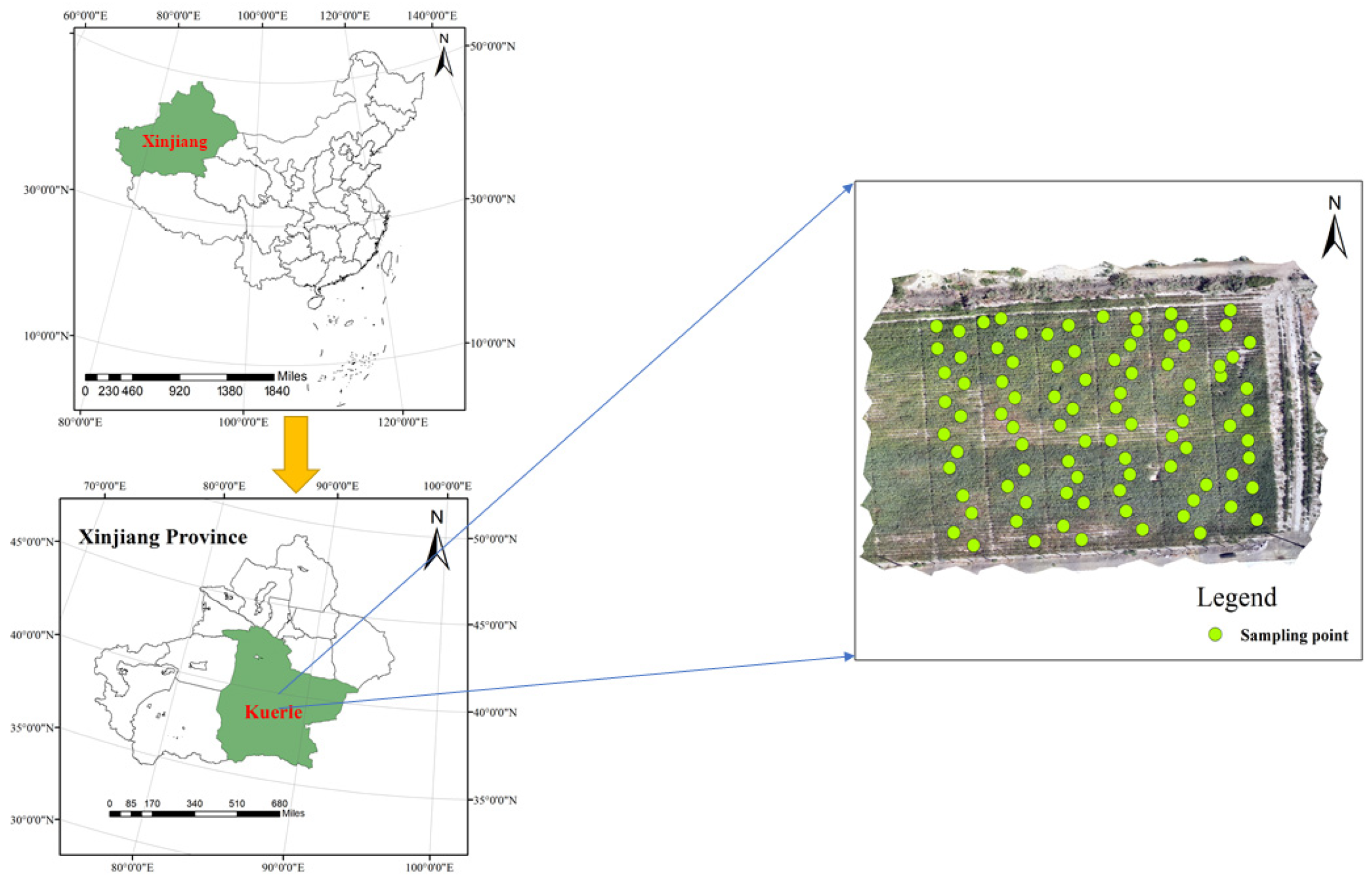
Figure 1. Experimental area.
Agriculture 15 02277 g001
Figure 2. Various degrees of mite infection on cotton leaves; the level is 0, 1, 2, and 3 in (ad), respectively.
Agriculture 15 02277 g002
Figure 3. Data collection: (a) MDG sample collection and (b) UAV data acquisition.
Agriculture 15 02277 g003
Figure 4. Data processing strategy.
Agriculture 15 02277 g004
Figure 5. Weights of the SHAP value.
Agriculture 15 02277 g005
Figure 6. SHAP values.
Agriculture 15 02277 g006
Figure 7. Flowchart of stacking.
Agriculture 15 02277 g007
Figure 8. Confusion matrices of the studied models (0: MDG_0 class, 1: MDG_1 class, 2: MDG_2 class).
Agriculture 15 02277 g008aAgriculture 15 02277 g008b
Figure 9. Spatial distribution map of cotton leaf mite damage grades based on the optimal classification model.
Agriculture 15 02277 g009
Figure 10. Model validation (0: MDG_0 class, 1: MDG_1 class, 2: MDG_2 class).
Agriculture 15 02277 g010
Table 1. Classification standard for spider mites.
Infestation ClassClassification Criteria
0No harm done
1Leaf blade intact; with sporadic white dots or with sporadic yellow spots on the bottom end of the leaf stem
2The leaf blade comprises less than one-third of the leaf area and is complete; seems slightly distorted or has noticeable yellow or red patches
3The cotton leaf has a large area of red or yellow spots that accounts for at least one-third of the leaf area, the leaf blade has a hole/holes or damage, or the leaf blade is twisted and distorted due to substantial damage
Table 2. UAV parameters.
Flight ParametersCamera Parameters
Takeoff weight1487 gFOV62.7°
Diagonal distance350 mmFocal length5.74 mm
Maximum flight height6000 mAperturef/2.2
Maximum ascent speed6 m/sRGB sensor ISO200–800
Maximum descent speed3 m/sMonochrome sensor gain1–8×
Maximum speed50 km/hMaximum image size1600 × 1300
Maximum flight time27 minPhoto formatJPEG/TIFF
Operating temperature0~40 °CFile system support≥32 GB
Operating frequency5.72~5.85 GHzOperating temperature0~40 °C
Table 3. Construction of vegetation indices.
NUMVegetation IndexFormulaReference
1NDVI(NIR − RED)/(NIR + RED)[26]
2GNDVI(NIR − GREEN)/(NIR + GREEN)[27]
3DVI-RNIR − RED[28]
4LCI(NIR − REG)/(NIR − RED)[29]
5MCARI2 3.75   N I R R E D 1.95     ( N I R G R E E N ) [ ( 2 N I R + 1 ) 2 ( 6 N I R 5 R E D 0.5 ) 0.5 ] 0.5 [30]
6VARI(GREEN − RED)/(GREEN + RED − BLUE)[31]
7SIPI2(NIR − GREEN)/(NIR − RED)[32]
8SAVI1.5(NIR − RED)/(NIR + RED + 0.5)[33,34,35]
9RDVI(NIR − RED)/(NIR + RED)1/2[36]
10WDRVI(0.2 ∗ NIR − RED)/(0.2 ∗ NIR + RED)[37]
11TDVI1.5 ∗ (NIR − RED)/(NIR ∗ NIR + R + 0.5)1/2[38]
12SRINIR/RED[39]
13MSRI(NIR/RED − 1)/(NIR/1)1/2 + 1[40]
14NLI(NIR ∗ NIR − RED)/(NIR ∗ NIR + RED)[41]
15MNLI-R1.5 ∗ (NIR ∗ NIR − RED)/(NIR ∗ NIR + R + 0.5)[42]
16GDVINIR − GREEN[43]
17ARI1(1/GREEN) − (1 REG)[44]
18ARI2NIR ∗ (1/GREEN − 1/REG)[44]
19CI-GREEN(NIR/GREEN) − 1[28]
20CI-ReEdge(NIR/REG) − 1[28]
21GARI N I R [ G R E E N 1.7     ( B L U E R E D ) ] N I R + [ G R E E N 1.7     ( B L U E R E D ) ] [45]
22GOSAVI(NIR − GREEN)/(NIR + GREEN + 0.16)[46]
23NDREI(REG − GREEN)/(REG + GREEN)[47]
24BNDVI(NIR − BLUE)/(NIR − BLUE)[48]
25CI-RED(NIR/RED) − 1[49]
26CVI(NIR/GREEN) ∗ (RED/GREEN)[50]
27DVI-GNIR − GREEN[27]
28DVI-RENIR − REG[27]
29EVI2.5 ∗ (NIR-RED)/(1 + NIR − 2.4*RED)[51]
30EVI22.5 ∗ (NIR-RED)/(1 + NIR + 2.4*RED)[52]
31GRVI(GREEN − RED)/(GREEN + RED)[53]
32MCARI11.2 ∗ [2.5 ∗ (NIR − RED) − 1.3(NIR − GREEN)][30]
33MCARI[(REG − RED) − 0.2(REG − GREEN) ∗ (REG/RED)][54]
34MNLI-G(1.5 ∗ NIR2 − 1.5 ∗ GREEN)/(NIR2 + RED + 0.5)[55]
35MSR[(NIR/RED) − 1]/[(NIR/RED) + 1]0.5[42]
36MSR-REG[(NIR/REG) − 1]/[(NIR/REG) + 1]0.5[40]
37MTCI(NIR − REG)/(NIR − RED)[56]
38NDRE(NIR − REG)/(NIR + REG)[57]
39NAVI1 − (RED/NIR)[58]
40OSAVI1.6 ∗ [(NIR − RED)/(NIR + RED + 0.16)][59]
41OSAVI-G1.6 ∗ [(NIR − GREEN)/(NIR + GREEN + 0.16)][36]
42OSAVI-REG1.6 ∗ [(NIR − REG)/(NIR + REG + 0.16)][60]
43RDVI-REG(NIR − REG)/(NIR + REG)1/2[61]
44RGBVI(GREEN2 − BLUE ∗ RED)/(GREEN2 + BLUE ∗ RED)[62]
45RTVI-CORE100(NIR − REG) − 10(NIR − GREEN)[63]
46SAVI-G1.5 ∗ (NIR − GREEN)/(NIR + GREEN + 0.5)[64]
47S-CCCINDRE/NDVI[65]
48SIPI(NIR − BLUE)(NIR − RED)[66]
49SR-REGNIR/REG[67]
50TCARI3[(REG − RED) − 0.2(REG − GREEN) ∗ (REG/RED)][68]
51T/OTCARI/OSAVI[69]
52TVI0.5[120(NIR − GREEN) − 200(RED − GREEN)][70]
Table 4. Classifier hyperparameters for optimal parameters.
ModelHyperparameter Optimization RangeOptimal Parameters
RFn_estimators: range (1, 200, 5)
min_samples_leaf: range (1, 10, 1)
min_samples_split: range (2, 10, 1)
max_depth: range (1, 30, 3)
max_features: range (1, 10, 1)
n_estimators = 45
max_depth = 6
min_samples_leaf = 6
min_samples_split = 2
max_features = 1
random_state = 5
SVMkernel: [‘linear’, ‘poly’, ‘rbf’, ‘sigmoid’]
C: [0.01, 0.1, 1, 10, 100]
gamma: [0.125, 0.25, 0.5, 1, 2, 4, 8, 16, 32, 64, 128]
kernel = ‘poly’
C = 100;
gamma = 4
DTcriterion: ‘gini’, ‘entropy’
max_depth: [3, 5, 8, 15, 25, 30, None]
min_samples_leaf: [1, 2, 5, 10]
min_samples_split: [2, 5, 10, 15, 100]
criterion: ‘gini’
max_depth = 1
min_samples_leaf = 1
min_samples_split = 2
random_state = 5
GBDTn_estimators: range (1, 50, 2)
max_depth: [2, 3, 4, 5, 6]
min_samples_split: range (2, 20, 2)
min_samples_leaf: range (1, 15, 1)
max_features: range (1, 5, 1)
subsample: [0.2, 0.3, 0.4, 0.5, 0.6, 0.7, 0.8]
n_estimators = 11
max_depth = 2
min_samples_split = 2
min_samples_leaf = 7
max_features = 4
subsample = 0.2
random_state = 5
XGBn_estimators: [30, 50, 100, 300, 500, 1000, 2000]
max_depth: [1, 2, 3, 4, 5, 6, 7, 8]
learning_rate: [0.01, 0.05, 0.1, 0.2, 0.3, 0.4, 0.5]
gamma: [0.1, 0.2, 0.3, 0.4, 0.5, 0.6, 0.7, 0.8, 0.9, 1]
reg_alpha: [0.0001, 0.001, 0.01, 0.1, 1, 100]
reg_lambda: [0.0001, 0.001, 0.01, 0.1, 1, 100]
min_child_weight: [2, 3, 4, 5, 6, 7, 8]
colsample_bytree: [0.6, 0.7, 0.8, 0.9]
subsample: [0.6, 0.7, 0.8, 0.9]
scale_pos_weight = 1
n_estimators = 8
max_depth = 2
learning_rate = 0.05
gamma = 1
reg_alpha = 0.0001
reg_lambda = 1
colsample_bytree = 0.75
min_child_weight = 1
subsample = 0.9
random_state = 5
KNNn_neighbors = range [1, 10]
weights = [‘uniform’, ‘distance’]
p = range [1, 5]
n_neighbors = 9
p = 3
weights = distance
LGBMmax_depth: range (2, 30, 1)
num_leaves: range (2, 12, 1)
min_data_in_leaf: range (1, 102, 10)
max_bin: range (5, 256, 10)
feature_fraction: [0.6, 0.7, 0.8, 0.9, 1.0]
bagging_fraction: [0.6, 0.7, 0.8, 0.9, 1.0]
bagging_freq: range (0,81, 10)
lambda_l1: [1 × 10⁻⁵, 1 × 10⁻³, 1 × 10⁻¹, 0.0, 0.1, 0.3, 0.5, 0.7, 0.9, 1.0]
lambda_l2: [1 × 10⁻⁵, 1 × 10⁻³, 1 × 10⁻¹, 0.0, 0.1, 0.3, 0.5, 0.7, 0.9, 1.0]
min_split_gain: [0.0, 0.1, 0.2, 0.3, 0.4, 0.5, 0.6, 0.7, 0.8, 0.9, 1.0]
n_estimators: range (1, 100, 5);
learning_rate: [0.008, 0.01, 0.02, 0.03, 0.04, 0.06, 0.08, 0.1]
max_depth = 2
num_leaves = 4
min_data_in_leaf = 41
max_bin = 55
feature_fraction = 0.9
bagging_fraction = 0.6
bagging_freq = 10
lambda_l1 = 1 × 10⁻⁵
lambda_l2 = 1 × 10⁻⁵
min_split_gain = 0.4
n_estimators = 100
learning_rate = 0.01
random_state = 5
Table 5. Single-model classification results.
ModelAccuracyMacro AvgWeighted Avg
PrecisionRecallF1PrecisionRecallF1
RF0.7780.9010.5810.6120.8440.7780.744
GBDT0.8100.5830.5830.5710.7460.8100.762
SVM0.7620.6900.6400.6550.7490.7620.752
XGB0.8250.9220.6910.6580.8260.8250.796
DT0.7940.5780.5670.5570.7370.7940.754
LGBM0.7460.7220.7910.7120.8450.7460.773
KNN0.7940.8110.6740.7170.8100.7940.783
Table 6. Results of the stacked models with a single base model.
Base ModelMetamodelAccuracyMacro AvgWeighted Avg
PrecisionRecallF1PrecisionRecallF1
XGBXGB0.8250.9220.6910.6580.8260.8250.796
GBDT0.5710.1900.3330.2420.3260.5710.416
DT0.8250.9220.6910.6580.8260.8250.796
KNN0.8250.9220.6910.6580.8260.8250.796
LR0.8100.5830.5830.5710.7460.8100.762
GBDTXGB0.7940.5780.5670.5570.7370.7940.745
GBDT0.5710.1900.3330.2420.3260.5710.416
DT0.7940.5780.5670.5570.7370.7940.745
KNN0.7940.5780.5670.5570.7370.7940.745
LR0.7940.5780.5670.5570.7370.7940.745
DTXGB0.7940.5780.5670.5570.7370.7940.745
GBDT0.5710.1900.3330.2420.3260.5710.416
DT0.7780.7180.6720.6850.8050.7780.781
KNN0.7940.5780.5670.5570.7370.7940.745
LR0.7940.5780.5670.5570.7370.7940.745
KNNXGB0.7940.8890.6670.7240.8300.7940.779
GBDT0.5710.1900.3330.2420.3260.5710.416
DT0.7940.8890.6670.7240.8300.7940.779
KNN0.7940.8890.6670.7240.8300.7940.779
LR0.7940.8890.6670.7240.8300.7940.779
Table 7. Results of the stacked models with multiple base models.
Base ModelMetamodelAccuracyMacro AvgWeighted Avg
PrecisionRecallF1PrecisionRecallF1
XGBXGB0.8250.9220.6310.6580.8660.8250.796
GDBTGDBT0.5710.1900.3330.2420.3270.5710.416
DTDT0.8250.9220.6310.6580.8660.8250.796
KNN0.8250.9220.6310.6580.8660.8250.796
LR0.8100.9170.6140.6440.8570.8100.779
XGBXGB0.8250.9220.6310.6580.8660.8250.796
GDBTGDBT0.5710.1900.3330.2420.3270.5710.416
KNNDT0.8570.9330.7260.7820.8860.8570.847
KNN0.8100.9170.6760.7360.8570.8100.795
LR0.8250.9220.6310.6580.8660.8250.796
GDBTXGB0.8250.9220.6310.6580.8660.8250.796
DTGDBT0.5710.1900.3330.2420.3270.5710.416
KNNDT0.7940.9120.6600.7190.8480.7940.776
KNN0.7780.9070.6120.6640.8400.7780.753
LR0.7620.9020.5950.6460.8320.7620.764
XGBXGB0.8410.9280.7100.7670.8410.8590.830
GDBTGDBT0.5710.1900.3330.2420.3270.5710.416
DTDT0.8570.9330.7260.7820.8860.8570.847
KNNKNN0.8100.9170.6760.7360.8570.8100.795
LR0.8410.9280.6790.7270.8760.8410.823
Table 8. Results from stacked models for double base models.
Base ModelMetamodelAccuracyMacro AvgWeighted Avg
PrecisionRecallF1PrecisionRecallF1
XGBXGB0.8100.5830.5830.5710.7460.8100.762
GBDTGBDT0.5710.1900.3330.2420.3260.5710.416
DT0.8250.9220.6910.6580.8260.8250.796
KNN0.8250.9220.6910.6580.8260.8250.796
LR0.8100.5830.5830.5710.7460.8100.762
XGBXGB0.8250.9220.6910.6580.8260.8250.796
DTGBDT0.5710.1900.3330.2420.3260.5710.416
DT0.8250.9220.6910.6580.8260.8250.796
KNN0.8100.9170.6140.6440.8570.8100.780
LR0.8100.9170.6140.6440.8570.8100.780
XGBXGB0.8250.9220.6310.6580.8660.8250.796
KNNGBDT0.5710.1900.3330.2420.3270.5710.416
DT0.8570.9330.7260.7820.8860.8570.847
KNN0.8410.9280.7100.7670.8760.8410.830
LR0.8250.9220.6310.6580.8660.8250.796
GBDTXGB0.7940.5780.5670.5570.7370.7940.745
DTGBDT0.5710.1900.3330.2420.3260.5710.416
DT0.7780.7180.6780.6850.8050.7780.781
KNN0.7780.7300.6720.6910.8000.7780.778
LR0.7780.5730.5500.5420.7290.7780.729
GBDTXGB0.7460.5410.5240.5140.6930.7460.696
KNNGBDT0.5710.1900.3330.2420.3260.5710.416
DT0.7940.8890.6670.7240.8300.7940.779
KNN0.8570.9180.7340.7820.8750.8540.846
LR0.7780.9070.6430.7010.8400.7780.757
DTXGB0.7780.8840.6190.6680.8210.7780.756
KNNGBDT0.5710.1900.3330.2420.3270.5710.416
DT0.7940.9120.6600.7190.8480.7940.776
KNN0.8410.9280.7100.7670.8760.8410.830
LR0.7780.9070.6120.6640.8400.7780.753
Table 9. Stacking integration with different construction methods.
Integration MethodBase ModelMetamodelAccuracyMacro AvgWeighted Avg
PrecisionRecallF1PrecisionRecallF1
Stacking (use_probas)XGB
GDBT
DT
KNN
LR0.8250.9220.6620.7120.8250.7300.807
Stacking (make_pipeline)XGB
KNN
DT0.8250.9220.6310.6580.8660.8250.796
Disclaimer/Publisher’s Note: The statements, opinions and data contained in all publications are solely those of the individual author(s) and contributor(s) and not of MDPI and/or the editor(s). MDPI and/or the editor(s) disclaim responsibility for any injury to people or property resulting from any ideas, methods, instructions or products referred to in the content.