Predictive Modelling of Maize Yield Under Different Crop Density Using a Machine Learning Approach

Abstract

In the face of increasing climate variability, understanding the dynamics of plant-to-plant interactions within crops is becoming increasingly important. This study aimed to examine plant responses to varying intensities of inter-plant competition, induced bz different planting densities, to enhance the accuracy of future yield prediction models. Six hybrids were grown at three planting densities (S1, S4, S7). Grain yield and yield components were estimated at four developmental points during grain filling (V1 to V4). These regression models and machine learning (ML) were applied to predict maize production under variable weather conditions. The factor year was the main source of variability, with less favourable conditions in the second year (G2) reducing yield by approximately 1–2%. Lower planting density (S1) improved individual plant development and yield components, while maximum density (S7) resulted in higher grain yield despite reduced individual performance. Hybrid H5 showed strong tolerance to high density, producing the highest yield under S7 conditions. Machine learning models accurately predicted key seed quality traits—moisture, oil, and protein—with performance metrics exceeding 80% accuracy. Specifically, R² values reached 0.82 for moisture content and 0.77 for oil concentration, indicating strong predictive capability. These findings support careful selection of hybrids and optimal planting density strategies in future cropping systems to increase yield and maintain seed quality in different environments.

1. Introduction

Maize (Zea mays L.) is cultivated worldwide under a variety of environmental conditions, making it the most widely grown crop [1]. As global climate change reduces the optimal ecological conditions for crop production, the structure and distribution of plant species are changing. Managing the negative impacts of the newly developed conditions is a challenge for contemporary agriculture in order to preserve the current crop production structure and quantity.

Current efforts are mainly focused on introducing new cultivation methods [2,3]. The number of plants per unit area is the most important factor in crop production and a basic requirement for high yields. Obtaining plant density in the field is one of the most effective methods for increasing maize production per unit area [4]. The number of plants is determined by sowing, but realized plant density relies on factors such as germination and emergence, meteorological conditions, and cultivation techniques. Maize breeding programs have developed hybrids that achieve the best performance at specific plant densities [5]. In the era of maize hybrids, densities have increased significantly, from around 30,000 plants ha⁻¹ in the 1950s to over 80,000 plants ha⁻¹ in some growing areas today [6]. Maize hybrids of recent breeding cycles are more water-efficient, use mineral nutrients more rationally and efficiently, and tolerate higher planting densities compared to earlier generations of hybrids [7,8]. Advancements in the performance of newly developed hybrids significantly enhance crop yield while promoting sustainability by reducing resource wastage. This dual focus on productivity and sustainability is essential in light of climate change and shifting crop structures. By adopting innovative practices, the agricultural sector can foster resilience and adaptability, thereby ensuring long-term food security [9,10,11]. Recommended plant density for a specific hybrid depends on numerous factors, i.e., the length of the hybrid’s vegetation period, morphological characteristics, plant growth pattern, available soil moisture, soil fertility, sowing time, and crop management. However, increasing the number of plants per unit area has its positive and negative aspects. A high maize planting density leads to a reduction in ear length, weight and number of grains per row, and root area [12,13]. This reduction can ultimately affect overall yield, as the plants intensively compete for nutrients and water. As a result, farmers must find a balance between plant density and resource availability in order to optimize growth and output. On the other hand, numerous results support the statement that increasing the number of plants per unit area may increase yield per ha [14,15]. The genetic and biological mechanisms that regulate yield potential are clearly different from those that control density tolerance [16]. Therefore, the problem of plant number per unit area must involve multiple factors such as soil quality, water availability, and nutrient management, which are essential for plant health and productivity. Further research is essential to unravel these complex interactions and develop strategies that maximise yield without compromising plant density [17].

In recent decades, numerous researchers have focused their efforts on developing monitoring techniques aimed at predicting crop yields [18]. Early and accurate crop yield prediction benefits the entire agri-food production chain, including individual producers, the processing industries, and regional governments [19]. Timely and reliable crop forecasts are vital for strengthening national and international food security policies, which are crucial for market stabilization and intervention planning in countries [20,21,22]. Timely yield forecasts may help producers to optimize agronomic management practices [23,24] and support the agri-food industry to refine food processing, storage, transportation, and marketing strategies [19,25,26,27]. A statistical prediction technique employs linear regression for processing data on morphological traits, yields, and meteorological factors. The relationship between these data sets provides a better understanding of how different elements and their interactions affect individual parameters and yield [28,29,30,31]. Applying machine learning and algorithms to heterogeneous data sets from different sources allows for deeper analyses of complex relationships and factors and generating predictions about them [32,33,34]. Forecasts show that one-third of the variance in global crop production is explained by climatic factors [35]. Along with weather factors, vegetation indices (VI) are another variable in the ability to predict yields, in many studies [28,36,37,38]. Accurate yield forecasting is crucial for the entire agri-food supply chain. However, the scope and level of precision required vary depending on the specific problem being studied [39].

This study aims to generate various predictors for yield prediction by investigating how different crop densities affect maize seed morphological traits and grain yield. Integration of field data with machine learning for maize yield prediction should introduce novel and impactful aspects that enhance accuracy, robustness, and practical utility.

2. Materials and Methods

2.1. Field Experiment and Plant Material

The field trial was set up at the experimental fields of Maize Research Institute Zemun Polje (MRIZP) (44°52′00″ N, 20°19′00″ E), the vicinity of Belgrade, during 2023 and 2024. The experiment was established as a split-plot in the Randomised Complete Block Design (RCBD) model with three replications (

Table 1. Elements of the experimental plot.

Element	Details
Blocks (Replications)	3 total; arranged vertically in the field layout.
Subplots per Block	3 per block, each representing one planting density S1: 40,816 plant ha−1, S4: 69,686 plant ha−1, S7: 98,522 plant ha−1.
Hybrids per Subplot	6 plots (H1–H6), randomized within each subplot.
Elementary Plot Size	0.196 m2 to 0.198 m2 (varies slightly by density).
Row Structure	Each hybrid sown in 3 rows per plot.
Row Length	14 m to 14.21 m (varies slightly by density).
Inter-row Spacing	70 cm between rows.
Intra-row (Plant) Spacing	S1 = 35 cm, S4 = 20.5 cm, S7 = 14.5 cm.

).

As plant material, six hybrids of different maturity groups (FAO 400 and 500) released at MRIZP were selected for the field experiment (H1 to H6). Sowing of the trial was carried out in three different crop densities, corresponding to the minimum, optimal, and maximum number of plants for the hybrids used in the trial (S1, S4, S7) (Figure 1).

According to USDA-NRCS (1999) [40], the soil was a slightly calcareous Chernozem (

Table 2. Soil quality parameters.

Parameter	Value/Description
Soil Classification (USDA-NRCS)	Slightly calcareous Chernozem (Molcal silt loam)
Soil Taxonomy	Coarse-loamy, mixed, superactive, mesic Vitrandic Calcixerolls
Soil Layer Analyzed	0–30 cm
Organic Matter	3.1%
Total Nitrogen (N)	0.23%
Organic Carbon (C)	1.8%
Accessible Phosphorus (P)	13 mg per 100 g soil
Available Potassium (K)	30 mg per 100 g soil
Total Calcium Carbonate (CaCO3)	9.5%
Soil pH	7.8
Soil Characteristics	Strong porosity, ideal heat and moisture regimes, high productive potential for maize and other cultivated crops
Source	USDA-NRCS (1999)

). This type of soil is characterized by strong porosity, ideal heat and moisture regimes, and a great potential for producing maize and other cultivated plants.

Conventional crop care and protection measures and soil cultivation were applied on the experimental plot during the growing season (

Table 3. Experimental field management.

Parameter	Details
Primary Tillage	Ploughing to a depth of 25–30 cm in autumn.
Seedbed Preparation	Spring tillage to a depth of 10–12 cm.
Fertiliser applied in Autumn	16.8 kg N ha−1 (2022)/18 kg N ha−1 (2023)
	67.2 kg P ha−1 (2022)/72 kg P ha−1 (2023)
	44.8 kg K ha−1 (2023)/36 kg K ha−1 (2023)
	Applied fertiliser: NPK 6:24:12; 300 kg ha−1
Fertiliser applied in spring	Applied fertiliser: Urea (46% N; carbamide); 280/300 kg ha−1
	280 kg ha−1 2023/300 kg ha−1 2024
Herbicide	Pre-emergence mixture: Adengo 0.44 L ha−1 + Glifomark 1.5 L ha−1.
	Post-emergence: Laudis 2 L ha−1

).

2.2. Chemical Analysis of Maize Kernels

Chemical analysis of maize kernels was performed using the non-destructive method Near-Infrared (NIR) spectroscopy to determine the content of starch (Skrob), protein (Protein), and oil (Ulja)) [40].

2.3. Grain Yield and Yield Components

Following ear harvesting, yield components were measured by creating ear samples from ten plants of each hybrid, with three replications. The samples were manually collected from each replication’s central row. The following traits were determined: CBL: cob length; NR: number of rows; NGR: number of grains per row; CBD: cob diameter; CCD: cob core diameter; CBM: cob mass; COM: cob core mass; MTG: mass of 1000 grains; and GY: grain yield. A calliper (accuracy 1/10 mm, range 0–150 mm; Kern, Ballingen, Germany) was used to measure the cob and the cob core diameter, and a precision meter was used for the cob length. The NR was counted on each cob from the sample, and the NGR was determined by counting three rows of grains on each cob. CBM was determined by weighing a sample of 10 cobs, which were crowned to measure COM, using a weighing scale (ET 1111, Technica, accuracy 0.01/01 g). The 1000-grain mass (MTG) was determined by the [41] International Seed Testing Association (ISTA) standard method.

The central row of each factor variant was harvested manually at the stage of full maturity to determine grain yield (YLD). Following the shelling of the cobs, the grain mass was measured. The values were then adjusted to a moisture content of 14% for the grain yield per hectare calculation.

The 15 days after pollination (DAP) stage and each subsequent 10-day interval are critical control points that coincide with key stages of grain development and grain filling. These parameters were monitored in the experiment as key points in the effective management of maize grain yield and quality. Grain filling monitoring and sampling were performed at stages V1: 15 (DAP), V2: 15–25 (DAP), V3: 25–35 (DAP), and V4: 35–45 (DAP).

Fifteen days after the pollination was finished, four sequential samplings were performed every ten days. Five plants from the third row were sampled in cycles called Time Treatments (V1–V4), which were used to evaluate SMZ—fresh grain mass, VSMZ—air-dry grain mass (60 °C); 105 mz—dry grain mass at temperature 105 °C. After removing the husk leaves, the seeds were taken from the ear cob, measured in a fresh state, and then dried in an oven (Memmert UN 110, Memmert GmbH, Schwabach, Germany) at a temperature of 60 °C for 24 h and 105 °C for 3 h.

2.4. Meteorological Conditions During the Experiment

The time frame during which the research was conducted (2023–2024) differed according to both observed parameters (temperature and precipitation). The first year of the research is characterised by higher precipitation and lower temperatures. Compared to the previous 30-year reference periods (1961-90-I, 1991-2000-II), the temperature in the growing season 2023–2024 increased by 1.6–3.8 °C and 2.8–5 °C, respectively. Precipitation in 2023 was lower by 7.7% and 52.6% compared to periods I and II, and in 2024 by 27.6% and 72.5%. Temperatures and precipitation were measured at the meteorological station of the Maize Research Institute Zemun Polje (

Table 4. Metrological data for the period 2023–2024.

	Monthly Mean Air Temperature (°C)
Year	April	May	June	July	Aug.	Sept.	Oct.	Average
2023	12.6	20.2	24.3	25.6	25.0	18.9	16.4	20.6
2024	16.52	19.21	24.98	27.45	27.87	20.92	15.92	21.8
Reference period of 30 years
I	11.4	16.6	19.6	21.1	20.6	16.9	11.5	16.8
II	13.6	18.2	21.9	23.8	23.7	18.5	13.3	19.0
	Monthly sum of precipitation (mm)
Year	April	May	June	July	Aug.	Sept.	Oct.	Sum
2023	64.9	94.6	63	66.7	58.2	54.3	23.6	425.3
2024	23.6	80.1	78.5	74.4	4	83.8	36	380.4
Reference period of 30 years
I	57.6	69.3	89.3	70.0	54.3	51.3	41.0	433.0
II	51.5	72.3	95.4	66.5	53.9	59.8	53.5	452.9

).

2.5. Statistical and Machine Learning Modeling

Measures of central tendency and measures of dispersion were used for data analysis. Data were analysed using the online application DataExplorer online [42] and locally adapted code in the Python programming language (version 3.12.0) with appropriate libraries for statistical data processing and machine learning (ML).

To evaluate the influence of three factors on grain moisture release parameters and yield, a three-way ANOVA was applied, where the factors analysed included the year of cultivation, planting density, and type of hybrid. Before conducting ANOVA, homogeneity of variance was checked using Levene’s test. In order to ensure the validity of the results, the normality of the data was checked using the Shapiro–Wilk test, which checked whether the data follow a Gaussian distribution. For post hoc analyses, Tukey’s HSD test was used. This test was applied to compare the means between all pairs of groups after a statistically significant difference was identified in the ANOVA analysis. In cases where the data violated the assumptions of normality or homogeneity of variances, the Kruskal–Wallis test was applied. For all statistical analyses, the level of significance p = 0.05 was used.

A principal component analysis (PCA) was used to fit the parameters to explore the main variances in the data and identify patterns between different factors. The results are presented through 2D and 3D PCA diagrams, which enable the visualization of the distribution of samples and the identification of key factors that influence variations in the data.

To evaluate the predictive potential of machine learning approaches, four regression models were applied: Linear Regression (LR), Quadratic Linear Regression (QLR), Random Forest (RF), and Extreme Gradient Boosting (XGBoost).

LR represents a fundamental statistical approach that models the relationship between input and target variables through a linear equation. QLR extends this concept by including polynomial terms, allowing the capture of moderate nonlinear dependencies. RF is an ensemble learning algorithm based on the aggregation of multiple decision trees trained on random subsets of data and features, providing improved predictive accuracy and robustness against overfitting. XGBoost is a gradient-boosting framework that sequentially builds decision trees, where each new tree corrects the errors of the previous ones through gradient optimization. It offers high performance on structured data and is particularly efficient for capturing complex nonlinear relationships. The selection of these algorithms ensured a balance between interpretability (LR, QLR) and predictive power (RF, XGBoost).

Categorical predictors (G, H) were one-hot encoded, while the numerical predictor (S) was retained in its original form. The dataset was divided into training (80%) and independent testing (20%) subsets using a random split with a fixed seed (random state = 42) to ensure reproducibility.

For model validation, a repeated 5-fold cross-validation with 10 repeats was performed on the training subset. This procedure provided reliable estimates of model stability and reduced the risk of overfitting. For each model, the mean R² across cross-validation folds (CV R²) and the R² value on the independent test set were determined. Models were then compared based on their cross-validation performance and independent test set R² values, and those with the most consistent and robust results were selected for further analysis.

To quantitatively evaluate model performance, several error-based metrics were employed, including the mean absolute error (MAE), mean bias error (MBE), root mean square error (RMSE), normalized root mean square error (NRMSE), and mean absolute percentage error (MAPE). These metrics are defined as follows:

$$MAE={\displaystyle \frac{1}{n}}\sum _{i=1}^n\left|y_i-{\widehat{y}}_i\right|$$

(1)

$$MBE={\displaystyle \frac{1}{n}}\sum _{i=1}^n\left(y_i-{\widehat{y}}_i\right)$$

(2)

$$RMSE=\sqrt{{\displaystyle \frac{1}{n}}\sum _{i=1}^n{\left(y_i-{\widehat{y}}_i\right)}^2}$$

(3)

$$NRMSE={\displaystyle \frac{RMSE}{\overline{y}}}\cdot 100$$

(4)

$$MAPE={\displaystyle \frac{100}{n}}\sum _{i=1}^n\left|{\displaystyle \frac{y_i-{\widehat{y}}_i}{y_i}}\right|$$

(5)

where $y_i$ and ${\widehat{y}}_i$ denote respectively the experimental (observed) and predicted values, $\overline{y}$ is the mean of observed values, and $n$ is the total number of data points.

In addition, model interpretability was addressed by analysing regression coefficients in the case of LR and QLR, while for RF and XGBoost, feature importance values and SHapley Additive exPlanations (SHAP) analyses were performed to quantify the contribution of each predictor variable to the model outputs.

Statistical and ML modelling were performed with the tools and support of the Atomistica.online platform (https://atomistica.online, accessed on 5 May 2025) [43,44,45,46,47].

3. Results

3.1. The Impact of Yield, Genotype and Density on the Expression of Average Yield Values and Yield Components

The highest average yield values were recorded for hybrid H5 across all three planting densities, suggesting a potential interaction between hybrid and density (S) and indicating that H5 is well-adapted to both low and high levels of crop competition. Morphological parameters related to the ear, including ear length, number of rows, number of grains per row, and ear weight, showed low to moderate standard deviation values, confirming good experimental reproducibility and consistent plant response or performance across treatments (Table S1.1).

Chemical grain parameters such as moisture content, protein levels, and starch and oil content showed low variability throughout the treatments (G-year, H-hybrids, S-density), indicating a high degree of homogeneity in the chemical composition of the grains within groups (Table S1.2).

Yield variability was moderate to high among different hybrids and planting densities. All tested hybrids achieved average yields ranging from 7.79 to 9.59 t/ha, with a coefficient of variation of less than 25%, indicating yield stability (Table S1.3).

Hybrids H5 and H6 showed the most favourable combination of high yield and low variability, while hybrid H1 expressed the highest variation (Table S1.3).

The mean values of the parameters SMZ, VZ, and 105 mz increase in later measurement terms (V1–V4), which indicates time-dependent changes that are statistically consistent. The standard deviation shows uniformity during all later terms (V2–V4), which suggests the same variability between samples over time (Table S1.4).

3.2. Assessment of the Influence of Year, Density and Hybrid on Yield and Yield Components

The significance of the examined factors was determined using three-factorial ANOVA. The normal distribution test results identified three parameters that were not suitable for ANOVA analysis. Parameters that did not meet the assumptions of normality and homogeneity (BR, BZR, and oil) were excluded from ANOVA (Table S2.1).

All three factors—year (G), density (S), and hybrid (H)—had a statistically significant effect on yield and yield components. The factor G exhibited the most substantial effect on the parameters PK, PKO, MK, MKO, M1000, moisture, proteins, starch, PVM, and PVK, which indicates that G is a significant source of variation. Factor density (S) affects several important components and quality traits (MK, MKO, PVM, PVK, starch, and protein), though its effect size appears smaller than G and H. Factor H demonstrated a statistically significant effect on nearly all parameters analysed, including DK, MKO, M1000, moisture, protein, and starch. Results indicate that the significant effects of the broad genetic influence of factor H imply that choosing the right hybrid matters for almost all traits. Among the interactions, G:H was significant for PRI, M1000, starch, and PVM, suggesting that the hybrid response varies across the cultivation years. Other interactions (G:S, S:H, G:S:H) did not reveal widespread significant effects on the parameters studied. The lack of significant interactions (G:S, S:H, G:S:H) implies that, for the majority of traits, hybrid and density effects are broadly consistent across environments. The statistical significance obtained by the analysis of variance justifies the choice of factorial variants and shows that the primary factors (G, S, H) can generally be treated independently in most cases. This independence simplifies the experimental design and allows for a clearer interpretation of the influence of each factor on the outcomes of the obtained results (

Table 5. The significance of the mean differences for grain yield and yield components.

Yield Components	p-Value
	G	S	H	G:S	G:H	S:H	G:S:H
DK	0.5310	<0.0001	<0.0001	0.0080	0.1950	0.8650	0.7440
PK	<0.0001	0.0650	0.0550	0.3770	0.2780	0.8400	0.5480
PKO	<0.0001	0.0950	0.0160	0.2900	0.7770	0.8030	0.8750
MK	<0.0001	0.0020	0.8480	0.0520	0.3520	0.7370	0.2880
MKO	<0.0001	0.0010	<0.0001	0.1460	0.2540	0.3100	0.2360
M1000	<0.0001	0.0120	<0.0001	0.1230	0.0190	0.0610	0.4000
Vlaga	<0.0001	0.5910	<0.0001	0.1700	0.1000	0.9220	0.6930
Protein	<0.0001	0.0340	<0.0001	0.0280	0.0590	0.9790	0.2230
Skrob	<0.0001	0.0010	<0.0001	0.0220	0.0440	0.7260	0.3920
PVM	<0.0001	0.0020	0.0010	0.1970	0.0040	0.4890	0.2330
PVK	<0.0001	0.0280	0.0010	0.6840	0.0220	0.6320	0.9630
PRI	0.6388	<0.0001	0.0021	0.7911	0.0071	0.4562	0.7871

Values of p < 0.05 are marked as statistically significant, while p < 0.0001 are marked as highly significant. DK—ear length, PK—ear diameter; PKO—ear core diameter; MK—ear mass; MKO—ear core mass; M1000—1000-kernel weight; Vlaga—moisture; Protein; Skrob—starch; PVM—height to tassel; PVK—height to ear; PRI—grain yield.

).

The Tukey HSD test revealed notable differences among specific groups of factors G, S, and H concerning the observed parameters. In DK, significant variations were identified between various planting densities (S1:S4 and S1:S7), in addition to differences among certain hybrids. For MK and MKO, marked differences were observed across cultivation years (G1:G2) and among individual hybrids. Furthermore, chemical grain parameters, including protein and starch content, exhibited significant differences across years (G1:G2), planting densities (S1:S7), and hybrids (Table S2.2).

Parameters that did not meet the assumptions of normality and homogeneity were analysed with the non-parametric Kruskal–Wallis test.

The Kruskal–Wallis test indicated a significant influence of factor H in all observed parameters except BR, where no statistical significance was recorded. Factor S showed a significant effect on BZR, while no statistical significance was found for the other parameters. On the other hand, the G factor had a statistically significant effect exclusively on the grain oil content (p < 0.0001) (

Table 6. Kruskal–Wallis test for yield and yield components by G, S, and H factors.

Parameter	Factor
	G	H	S
BR	0.124	<0.0001 **	0.8333
BZR	0.9877	0.0008	0.0002 *
Ulja	<0.0001 **	0.0057	0.7591

Values of * p < 0.05 are marked as statistically significant, while ** p < 0.0001 are marked as highly significant. BR—number of rows; BZR—number of grains per row; ulja—oil.

).

3.3. Multivariate Analysis of Yield, Yield Components and Chemical Grain Parameters

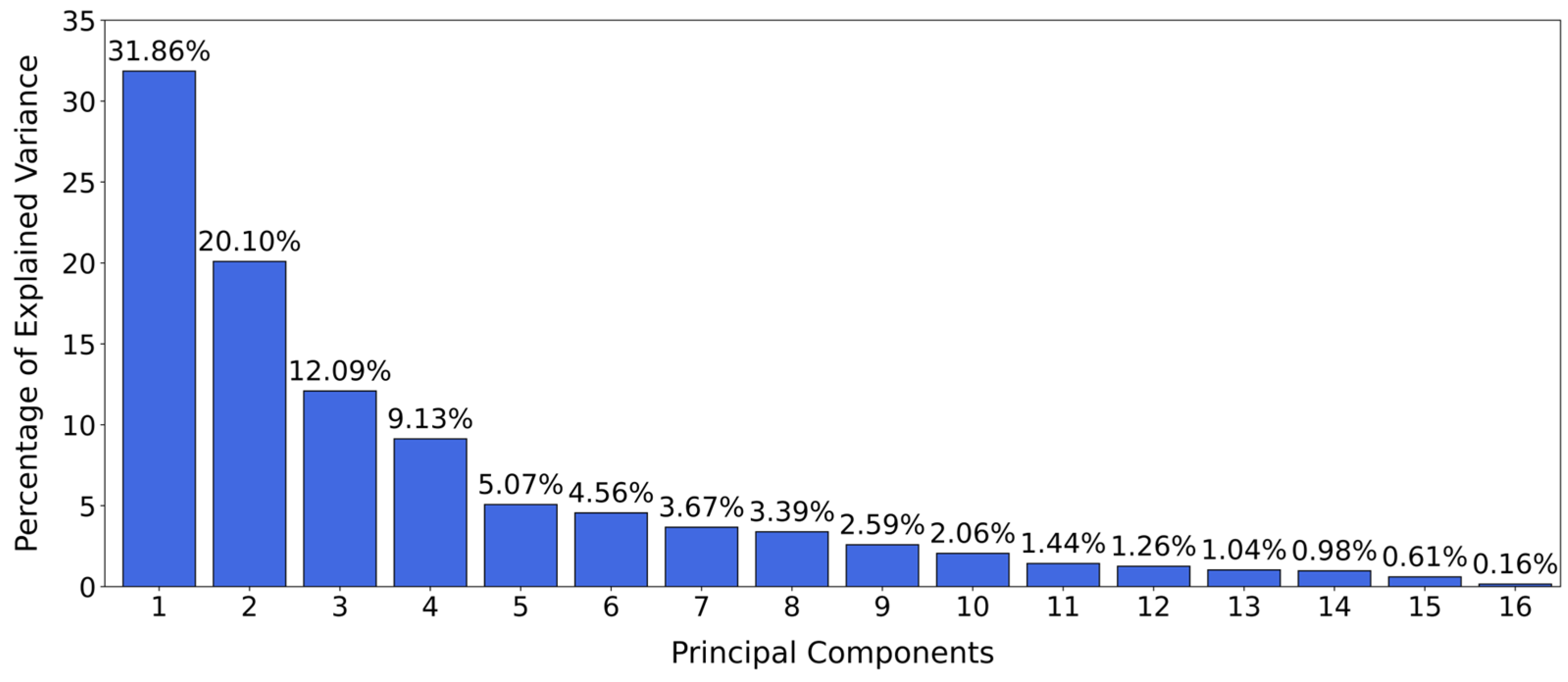
Principal component analysis (PCA) was utilized to examine the interrelationships among various samples. The initial three principal components explained 64.05% of the overall data variability regarding the yield, yield components, and chemical grain parameters (Figure 2).

Multivariate analysis, conducted within the PCA factor space, identified groups of traits based on the effects of year (G), hybrid (H), and planting density (S).

Regarding the production year factor (G), two clearly distinct variation groups were observed: G1 and G2. Group G1 had a dominant influence on yield, yield components, and grain chemical composition. In contrast, group G2 was associated with variability in BRZ and BZR, showing a negative correlation with starch accumulation. This may reflect the impact of environmental stress conditions that favour the formation of a higher number of grains at the expense of starch content per grain.

The planting density factor (S) showed moderate differences, particularly between groups S1:S4 and S7:S4. Although S4 remained undefined in relation to the other two densities, certain distinctions between S1 and S7 could be observed, especially in grain yield.

The hybrid factor (H) did not reveal clear differentiation, suggesting that the tested hybrids were phenotypically similar under the studied conditions. The absence of pronounced hybrid effects may indicate that the influence of year—and to a lesser extent, planting density—was substantially stronger than the effects attributable to hybrid variation (Figure 3e,f).

The Contribution of Traits to Particular Principal Component Variances.

The examination of vector lengths within the PCA framework revealed that the parameters MK, DK, MKO, BZR, and Moisture significantly influenced the differentiation of samples along the initial principal components (Table S3.1). Notably, moisture emerged as the most substantial contributor to the PC1 component, underscoring its critical role in distinguishing samples according to the primary variance direction. Furthermore, in relation to the contributions of the PC1 components, the M1000 and oil parameters were particularly prominent (Table S3.2).

Based on the 3D PCA analysis, the variables DK, BZR, PKO, and MK showed the largest total contributions in the principal components space (PC1–PC3), making them the most prominent for explaining the total variance of the data (Table S3.3). In addition, the variable Moisture had the largest single contribution to the PC1 component, thus confirming its key role in separating the samples along the main direction of variation (Table S3.4).

Considering the results of both 2D and 3D PCA analyses, the moisture parameter stood out as a variable of key importance for discriminating samples in principal component space.

3.4. Machine Learning (ML) Analysis for Predicting Yield and Yield Components

3.4.1. The Development of Predictive Models Utilizing Linear Regression

The predictive analysis for the data set “Yield, Yield component and Chemical grain parameters” was performed in relation to three predictors (G, H, S). For two parameters (moisture and oil), models of high accuracy and reliability (80%) were obtained, while the parameter protein achieved an accuracy limit of 50% (

Table 7. Model performance (test-set and CV R²) for predicting yield parameters based on G, S, and H.

Parameters	Model	R2	CV Mean R2
Vlaga	Linear Regression	0.8242	0.8920
Vlaga	Quadratic Linear Regression	0.7820	0.8570
Vlaga	Random Forest	0.7673	0.8391
Vlaga	XGBoost Regressor	0.7682	0.8405
Ulja	Linear Regression	0.7044	0.6850
Ulja	Quadratic Linear Regression	0.6839	0.6089
Ulja	Random Forest	0.6107	0.6111
Ulja	XGBoost Regressor	0.6786	0.6188
Protein	Linear Regression	0.4417	0.5048
Protein	Quadratic Linear Regression	0.2541	0.3910
Protein	Random Forest	0.3162	0.3904
Protein	XGBoost Regressor	0.2774	0.3757

The analysis was rated as acceptable for models with CV Mean R² ≥ 0.50, while models with CV Mean R² ≥ 0.80 were classified as excellent. The table shows only values for models whose CV Mean R² was ≥0.50. Models with CV Mean R² < 0.50 are due to insufficient predictive reliability. Vlaga—moisture; Ulja—oil; Protein—protein.

). The linear regression model appeared to be the most accurate approach and revealed that the PCA analysis successfully predicted the quantities most associated with the predictors.

Furthermore, there is currently no reliable and predictively applicable model for PRI utilizing these input predictors (G, H, S).

Among the modelled target variables, Vlaga (grain moisture content) and Ulja (grain oil content) demonstrated the most promising predictive performance across all applied ML models. In particular, LR achieved the highest independent test set R² values (0.824 for Vlaga and 0.704 for Ulja) and consistent cross-validation stability, outperforming more complex approaches such as random forest and XGBoost. By contrast, the prediction of protein content showed considerably weaker performance, with R² values not exceeding 0.45, indicating limited suitability of the selected descriptors for this property. Therefore, in the following sections we focus on Vlaga and Ulja as representative cases, providing a more detailed evaluation of their predictive models. For these two best-performing targets, additional error-based evaluation parameters (MAE, MBE, RMSE, NRMSE, and MAPE) are reported in a separate table to ensure a comprehensive assessment of accuracy and reliability.

According to the results presented in

Table 8. Error-based evaluation metrics (MAE, MBE, RMSE, NRMSE, and MAPE) for the two best-performing target variables (Vlaga and Ulja) obtained with the selected regression models.

Target	CV Mean R2	CV Std	Test R2	MAE	MBE	RMSE	NRMSE	MAPE (%)
Vlaga	0.8920	0.0382	0.8242	0.7072	0.0002	1.1162	0.0863	5.0431
Ulja	0.6854	0.1507	0.7044	0.2233	−0.0412	0.2811	0.0673	5.2367
Protein	0.5185	0.2461	0.4417	0.5227	−0.0049	0.6551	0.0659	5.3460

CV—coefficient of variation, MAE—Mean Average Error, MBE—Mean bias error, RMSE—Root Mean Squared Error, NRMSE—Calculates the Normalized Root Mean Squared Error, MAPE—Mean Absolute Percentage Error, grain moisture content (Vlaga), gain oil content (Ulja), grain protein content (Protein).

, Vlaga and Ulja are indeed two targets with reliable predictive performance. For Vlaga, the LR model achieved a high independent test set R² of 0.8242 with stable cross-validation (0.8920 ± 0.0382). The error parameters indicate excellent predictive quality, with low MAE (0.7072), minimal bias reflected in MBE (0.0002), and moderate absolute error as RMSE (1.1162). Both the relative error measures, NRMSE (0.0863) and MAPE (5.0431%), confirm robustness and accuracy. For Ulja, predictive performance was slightly lower but still satisfactory, with an independent R² of 0.7044 and a cross-validation mean of 0.6854 (±0.1507). Error analysis shows low MAE (0.2233), small negative bias (MBE = −0.0412), and low overall error (RMSE = 0.2811), with relative measures NRMSE (0.0673) and MAPE (5.2367%) confirming strong reliability.

To further illustrate the predictive relationship between the selected variables, the final regression equation for Vlaga is presented below, providing an interpretable representation of the contribution of each predictor (Equation (6)).

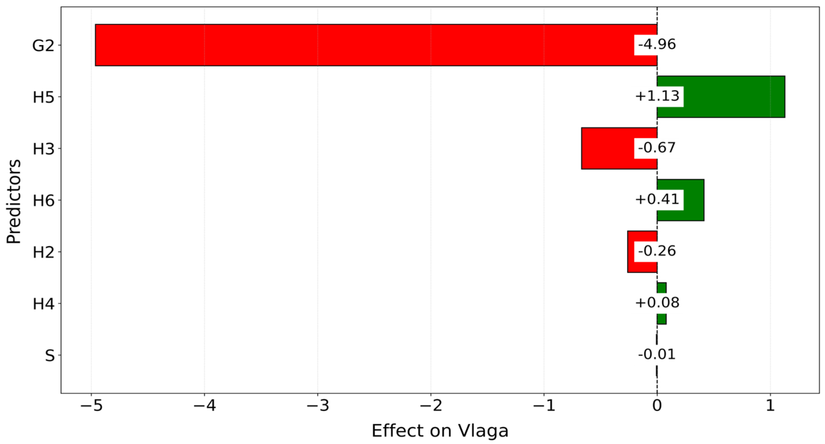
$$\begin{gathered} Vlaga=15.6219-4.9630·G2-0.2605·H2-0.6676·H3+0.0794·H4 + \\ 1.1284·H5+0.4142·H6-0.0068·S \end{gathered}$$

(6)

Examination of the key coefficients within the model shows that the year of production significantly affects the variation in grain moisture content. In this particular model, the difference between G1 and G2 is associated with an average decrease in moisture content of about 4.96 units. In addition, when considering the genotype-hybrid as a predictor in the prediction model, for hybrids H5 and H6, the estimate for grain moisture content shows an average increase of about 1.13 units, or 0.041, whereas hybrid H3 is linked to an average decrease in moisture by approximately 0.67 units. These findings suggest that the predicted moisture value is statistically more influenced by the experimental year and the selected hybrid than by the other predictors included in this model or crop density (Figure 4).

According to the results presented in Table 7, Ulja also demonstrated reliable predictive performance, although at a slightly lower level compared to Vlaga. The LR model achieved an independent test set R² of 0.7044, supported by a cross-validation mean of 0.6854 (±0.1507). The error parameters indicate satisfactory predictive quality, with low MAE (0.2233), a small negative bias reflected in MBE (−0.0412), and low absolute error as RMSE (0.2811). Both relative error measures, NRMSE (0.0673) and MAPE (5.2367%), further confirm the reliability and robustness of the model for predicting Ulja.

Same as for Vlaga, we are referring to the final regression equation for Ulja, providing an interpretable representation of the contribution of each predictor (Equation (7)).

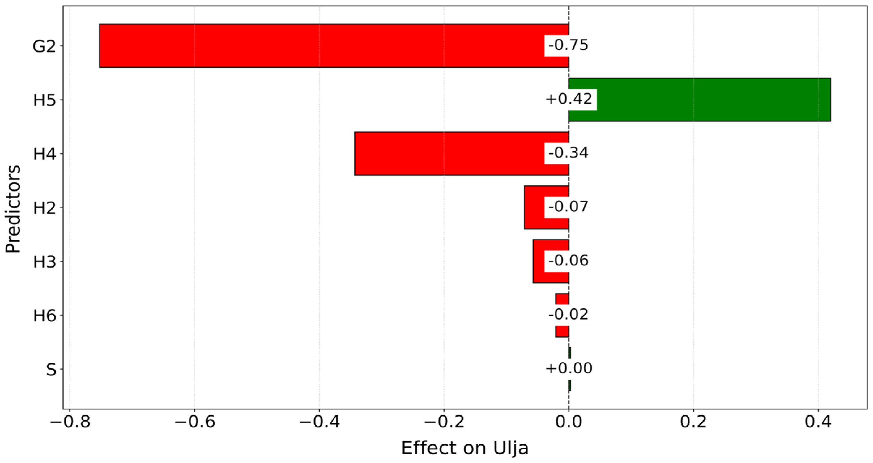
$$\begin{gathered} Ulja=4.5836-0.7521·G2-0.0712·H2-0.0569·H3-0.3430·H4 + \\ 0.4199·H5-0.0207·H6+0.0025 \end{gathered}$$

(7)

Examining the most prominent coefficients within the model reveals the significance of environmental conditions. Furthermore, the alteration in meteorological conditions during the vegetation season, particularly between the transition from G1 to G2, correlates with an average reduction in oil value of roughly 0.75 units. The findings from the projection of oil quantity in the grain, utilising the genotype (hybrid) as a predictor, clearly underscore the importance of this factor. Specifically, hybrid H5 shows an average increase in oil value of about 0.42 units, while hybrid H4 is associated with an average decrease in oil value of about 0.34 units. These results indicate that the year of the experiment and the choice of hybrid have a more pronounced statistical influence on the predicted oil value in relation to planting density (Figure 5).

The linear regression model created for analysing protein levels with the predictors G, S, and H yielded an R² value of 0.44. This indicates that roughly 44% of the variability in protein levels can be accounted for by the selected predictors (Table 7). Additionally, cross-validation resulted in an average R² of 0.50, which signifies a moderate degree of generalization performance. While the R² values do not suggest a fully dependable model, the cross-validation outcome and the slight difference in R² values between the test and cross-validation datasets imply that this model may possess some practical applicability, though it is limited.

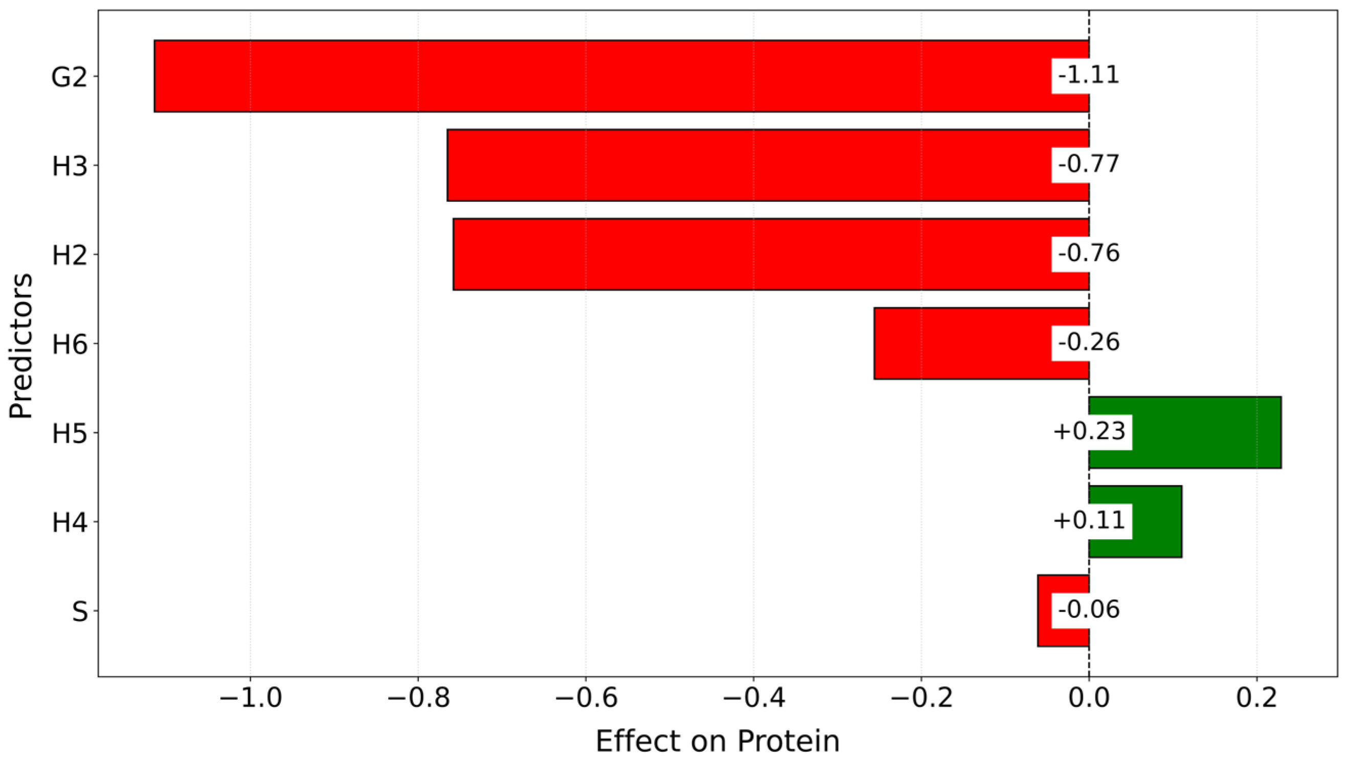
$$\begin{gathered} Protein=10.9944-1.1142·G2-0.7580·H2-0.7651·H3 + \\ 0.1104·H4+0.2289·H5-0.2561·H6-0.0611·S \end{gathered}$$

(8)

The analysis of the most important coefficients in the third prediction model indicates that, similar to previous models, the year of production significantly affected the variability of the protein trait. Furthermore, the production conditions during the transition from G1 to G2 were associated with an average reduction in protein values of about 1.11 units. The impact of different hybrids on the fluctuation of protein values varied according to their genetic foundation. Hybrid H3 exhibits an average decrease in protein of about 0.77 units, while hybrid H2 also corresponds to a decrease of roughly 0.77 units. Conversely, hybrids H4 and H5 demonstrate an increase in protein, with H5 showing a notably greater enhancement. These results imply that both the experimental year and the chosen hybrid have a statistically greater influence on the predicted protein value than does planting density, which appears to play a minor role according to this model (Figure 6).

3.4.2. Predictive Analysis of the Influence of G, H, and S on Moisture Release Parameters

PCA analysis identified grain moisture content as the primary factor influencing variability among all studied parameters. Based on this, moisture release properties (SMZ, VSMZ, 105 mz) were in the focus of predictive analysis. The predictive analysis of the “Moisture Release” dataset was conducted with respect to four predictors (G, H, S, and V), while all other numerical variables were treated as target variables. As in the case of the “Yield, Yield Component, and Chemical Grain Parameters” dataset, four ML models were tested against the target variables, and these results are summarized in Table S4.1.

Several target variables yielded models with exceptionally high accuracy and reliability. For the mentioned target quantities, in all cases the XGBoost machine learning model emerged as the most precise method, and PCA analysis effectively identified the maize characteristics most closely associated with the predictors. Notably, the model for the SMZ parameter exhibited remarkable performance, with R² (0.90) and CV Mean R² (0.93) values reflecting outstanding accuracy and consistency. Parameters—VSMZ and 105 mz—also achieved models with an accuracy of more than 80%. These models were subsequently analysed to elucidate the impact of the predictors on the measured variables (Table S4.1). Error-based parameters for these selected models are presented in

Table 9. Error-based evaluation metrics (MAE, MBE, RMSE, NRMSE, and MAPE) for the target variables (SMZ, VSMZ, and 105 mz) obtained with the XGBoost model.

Target	CV Mean R2	CV Std	Test R2	MAE	MBE	RMSE	NRMSE	MAPE (%)
SMZ	0.9346	0.0124	0.8975	4.3251	0.3572	5.4387	0.1514	13.7417
VSMZ	0.8952	0.0144	0.8625	2.2292	0.4112	2.8655	0.2583	29.6875
105 mz	0.8930	0.0153	0.8522	2.2307	0.4389	2.8498	0.2689	31.7272

CV—coefficient of variation, MAE—Mean Average Error, MBE—Mean bias error, RMSE—Root Mean Squared Error, NRMSE—Calculates the Normalized Root Mean Squared Error, MAPE—Mean Absolute Percentage Error, SMZ—Fresh Grain Mass, VSMZ—Air-dry Grain Mass, 105 mz—Grain mass after drying at 105 °C.

.

For SMZ, the model showed the most reliable results, with a high independent test set R² of 0.8975 and excellent cross-validation stability (CV mean R² = 0.9346, CV std = 0.0124). Error-based metrics further confirm accuracy, with low MAE (4.3251) and RMSE (5.4387), minimal bias (MBE = 0.3572), and acceptable relative error values (NRMSE = 0.1514, MAPE = 13.7417%). These results indicate that SMZ can be predicted with high confidence. For VSMZ, the model also performed well, with a test set R² of 0.8625 and a stable cross-validation mean of 0.8952 (±0.0144). Absolute error values were low (MAE = 2.2292, RMSE = 2.8655), while relative error measures (NRMSE = 0.2583, MAPE = 29.6875%) suggest that although the model successfully captured the underlying trend, small variations in the data may have contributed to slightly higher relative deviations. For 105 mz, predictive performance was comparable, with a test set R² of 0.8522 and cross-validation mean of 0.8930 (±0.0153). Absolute errors again remained low (MAE = 2.2307, RMSE = 2.8498), and relative errors (NRMSE = 0.2689, MAPE = 31.7272%) were somewhat higher but still within an acceptable range for complex biological datasets.

In the following section, we provide a more detailed analysis of these models, including an interpretation of feature importance and SHAP visualizations to better understand the contribution of individual predictors. We begin with a model for the SMZ parameter, whose results are summarized in Figure 7.

According to the results presented in Figure 7a, the main predictors identified are G and V. Notably, G2 and V4 each play a significant role in enhancing the model’s accuracy, exceeding 0.45. This indicates that the year of the experiment (G2) and the timing of sampling and measurement (V4) are crucial for predicting the SMZ value, with a joint significance level greater than 90%. According to the SHAP analysis presented in Figure 7b, V4 contributed to the increase of SMZ values for the mean value of 20 units, positioning it as the second most critical temporal factor. V2 and V3 exhibited a weak positive influence on SMZ. The predictor H provided a smaller yet noticeable contribution to the variability of SMZ. The other predictors demonstrate minimal relevance, and their effect on SMZ prediction is negligible when compared to G2 and V4. The mean values of the factor S are mostly at zero, indicating that it did not influence the change in the value of the SMZ. Other predictors also showed negligible influence on SMZ.

In Figure 8, we have summarised the feature importance and SHAP analysis in the case of the model for the VSMZ parameter.

According to the results presented in Figure 8a, the primary determinant for the VSMZ parameter was G2, which played a crucial role in enhancing the model’s accuracy, exhibiting an importance level exceeding 0.5, thereby underscoring the substantial impact of the second year of the experiment. The V4 ranked as the second most influential Time Treatments predictor, offering a moderate contribution, whereas V3 and V2 also add value to the model, although to a lesser degree. Conversely, all other predictors, including S and H of maize, held minimal relevance in this model with no significant contribution in forecasting the VSMZ value (Figure 8a).

According to the SHAP analysis presented in Figure 8b, predictor G2 has an extremely positive influence on the value of VSMZ. Of the Time Treatments predictors, V4 has the strongest positive influence on the VSMZ parameter, while both V3 and V2 show a moderate contribution to the increase. This trend is consistent with previous observations and points to a temporal component as an important factor. Hybrid H6 has a relatively pronounced negative impact, reducing the value of VSMZ. In certain other instances involving the application of the hybrid H5, a beneficial contribution was noted, suggesting a potentially favourable influence of the factor H. The predictor S exhibited a neutral effect in the majority of cases, with minor fluctuations in both directions (Figure 8b).

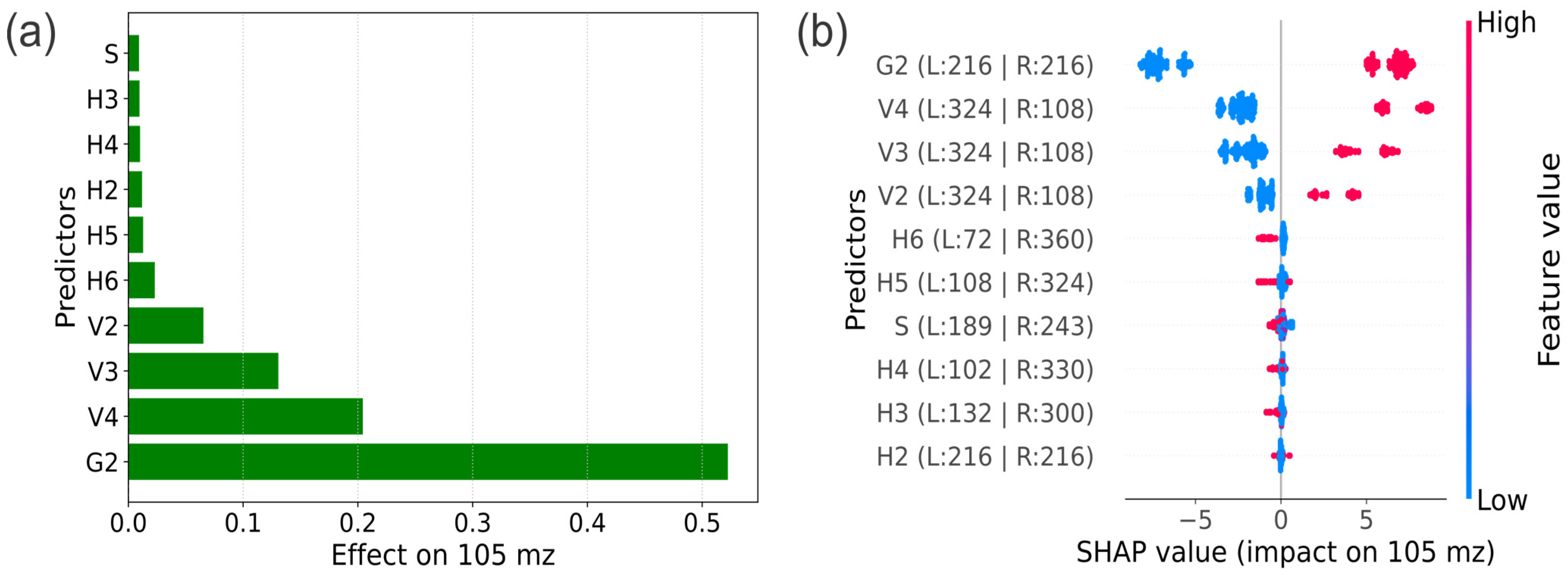
Finally, in Figure 9 we are presenting feature importance and SHAP analysis in the case of the model for predicting the 105 mz parameter.

The feature importance in the case of the model for the 105 mz parameter (Figure 9a) indicates that the primary predictors were G and V. Variation in the levels of these factors leads to measurable differences in the variable. Factor G2 emerged as the most critical predictor influencing the model’s accuracy, followed by V4 as the second most significant predictor. Additionally, V3 and V2 provided some contribution, whereas the predictors related to hybrids and planting density were of minimal relevance in comparison to those previously identified (Figure 9a).

According to the SHAP analysis for the model related to 105 mz parameter (Figure 9b), the presence of predictor G2 has evidently resulted in an increase of the 105 mz parameter. The SHAP values associated with G2 were consistently positive, ranging from approximately +5 to +7.5, which signified a reliable positive influence of the second year on the variable 105 mz. Predictors V4, V3, and to a lesser extent V2, exhibited a trend towards increasing the value at 105 mz, with V4 making the most significant contribution, characterized by its notably positive SHAP values. V4 expressed a pre-dominantly positive effect, while V3 offered a moderate positive contribution. On the other hand, V2 had a weak impact. In contrast, the factors H and S showed a variable influence, with some leading to an increase in a on the one hand, and a decrease in the value to 105 mz on the other hand. Additionally, predictor S played a dual role, contributing to both the increase and decrease of the 105 mz parameter.

4. Discussion

4.1. The Impact of Yield, Hybrid and Density Factors on the Expression of Average Yield Values and Yield Components

Developing hybrids that can withstand high plant density and applying suitable crop management techniques can alleviate the negative impacts associated with increased plant density [48,49]. A two-year study revealed that the year of production, planting density, and hybrid significantly impact yield and its components, with the relationship between yield and plant density being complex and influenced by several interacting variables [50].

Studies indicate that a reduction in precipitation in the second production year—G2—during the winter (84.4 mm) and growing season (44.9 mm), combined with an increase in temperature of approximately 2.7 °C during the sowing–emergence–fertilisation period, can reduce yield by 1–2%. This decline is accompanied by reductions in grain weight, grain number, protein and oil content, and other traits such as DK, MK, MKO, M1000, VL, PVM, and PVK. These findings emphasise the need to regulate both the amount and timing of precipitation as well as the temperatures during critical growth stages.

Maitah et al. [51] reported a moderate to strong positive correlation between maize yield and July precipitation (r = 0.54–0.79) and a negative correlation with mean August temperatures (r ≈ −0.4 to −0.5). Under elevated temperature stress, yield losses can reach 30–40%, significantly impacting the expression of yield-related traits [52].

In response to plant density, yield, yield components, and chemical grain parameters followed a normal distribution. Increasing density to 98,522 plants ha⁻¹ resulted in higher yield, while other traits reached optimal values at lower, less competitive densities (e.g., 40,816 plants ha⁻¹). The interaction between year and planting density significantly influenced the chemical composition of seeds, including VL, Protein, Ulja (oil), Skrob (starch), VM, and PVK.

However, certain traits such as ear length and weight showed minimal variability across environments, indicating stability. In this context, hybrids H1 and H6 demonstrated greater stability for traits such as DK, BRZ, MK, MKO, and VL, whereas H2 and H3 showed higher variability, as reflected in their DK, PKO, and MK values.

4.2. Multivariate Analysis of Yield and Yield Components

Principal component analysis (PCA) revealed patterns in trait behaviour by year (G) and density (S), while hybrid (H) showed minimal differentiation. The strongest phenotypic shifts—particularly in traits such as starch (Skrob), BRZ, BZR, and PKO—were observed between years, reflecting significant environmental influence on trait expression [53,54,55,56]. This aligns with Jiang et al. [57], who used PCA to improve yield and protein predictions via vegetation indices across growth stages, reinforcing the value of environment-aware strategies and hybrids that can adapt to changing environments [58]. Yield response to density was shaped by environmental conditions and plant interactions. Planting density showed minimal differentiation of traits based on different plant numbers in the experiment. This underscores the complexity of ecological dynamics, where multiple factors can either enhance or diminish trait effects. Understanding these interactions is vital for optimising crop productivity and sustainability [59,60].

These findings support earlier research on genotype × environment × management (G × E × M) interactions. Lobel et al. [61] and Rufo et al. [62] emphasised that the benefits of higher density depend on environmental stress and complementary management practices. Thus, plant density reflects the system’s ecological “carrying capacity” and must be optimised in relation to hybrid choice, soil, and water availability [63].

4.3. Machine Learning (ML) Analysis for Predicting Yield and Yield Components

Yield prediction models are often unreliable because yield is influenced by changes in meteorological conditions, differences in soil composition, the response of hybrids to different environments, and the interactions among these factors. In comparison, seed quality traits were easier to predict since they had more stable relationships with the available variables.

The integration of machine learning with large agricultural datasets has great potential to reveal patterns, though predictive accuracy often suffers due to high data variability [64,65,66]. However, when data from multiple phenological stages are included, a more complete picture of maize development emerges [67,68]. Among various models tested, linear regression provided the most accurate predictions for grain properties based on experimental data. Three maize grain traits—moisture, oil content, and protein—were reliably predicted, while models for other traits and overall yield were less dependable.

In this study, year of production and plant density were the most significant predictors of maize grain moisture. Jiang et al. [67] found that sowing date, hybrid type, and environmental factors such as density significantly influenced maize kernel moisture dynamics. Environmental conditions like humidity and temperature during the growing season greatly affect initial grain moisture content due to the hygroscopic nature of maize kernels and their tendency to gain or lose moisture until they reach equilibrium with ambient air [69].

Further analysis of moisture release revealed highly accurate models (>80%) for SMZ, VSMZ, and 105 mz. The production year appeared to be a key factor affecting grain moisture dynamics in all predictive models. In both agricultural engineering and food science, understanding moisture kinetics during drying is essential for improving product quality. As such, machine learning is increasingly used to estimate maize moisture content [54,70] and determine the optimal timing for harvest as a crucial step for seed quality enhancement.

The model further indicates different levels of effects of the genotype factor, predicting a positive contribution of H5 (+0.42 units) and a negative contribution of genotype H4 (–0.34 units) to grain oil content. These findings are consistent with factorial regression and AMMI analyses, confirming that environmental variability and genotype–environment interactions have a significantly greater impact on grain oil and protein content than agronomic factors such as planting density [71,72,73]. The linear regression model for oil prediction is comparable to results reported in soybean oil content prediction models, which often show predictive accuracy in the range of 0.6–0.8 under similar modelling approaches [73,74].

Analysis of key coefficients in the third predictive model for protein content shows that year of production significantly influenced the variability of protein, which is consistent with the findings reporting highly significant main and interaction effects of year and genotype on grain protein content (p < 0.01) [75,76].

The predictive power of the third model is comparable to accepted field reference values [77]. Although not high enough for accurate individual prediction of grain protein content in maize, it is useful for screening or trend analysis, especially when used in breeding or agronomic optimisation. Analysis of the regression coefficients in King et al. [78], in models that included genotype and environmental factors, reveals that the R² values of the regression coefficients are in the range of 0.49, which is almost identical to the performance of the results presented in this paper.

Planting density can affect yield components; its effect on protein concentration is usually indirect.

The limited effect of crop density is in accordance with the agronomic literature. Protein concentration is more sensitive to genetic and environmental factors than to the number and arrangement of plants, as confirmed by the results of Laidig et al. and King et al. [79,80], where density is not recognised as a reliable predictor in the regression models for protein.

While machine learning offers powerful tools for seed yield prediction, the reliability still heavily depends on data quality, model choice, and understanding of underlying biological and environmental processes. To enhance the reliability and accuracy of yield prediction models, future work should be based on combining machine learning with domain expertise and high-quality, comprehensive data.

5. Conclusions

The study examined the influence of different factors (G, H, S) on yield, yield components, and chemical grain parameters in six maize hybrids. The highest average yield was recorded for the H5 hybrid at the S1 planting density, indicating that H5 performs best under conditions of reduced resource competition. This hybrid consistently demonstrated superior performance across all years and densities examined, making it an excellent candidate for production in the diverse agro-climatic environments.

This research identified seed moisture content as the key trait for predicting maize yield patterns, significantly influenced by G and to a lesser extent by S. This conclusion was supported by regression and machine learning methods, which highlighted its role in distinguishing between samples.

Different machine learning models showed significant variability depending on the selected predictors. Reliable prediction models were obtained for the relationship between moisture, oil, and protein in relation to G, H, and S factors. The results showed a high level of predictive accuracy for moisture and oil, highlighting the importance of experimental year and hybrid selection. This study’s ML approach provides a useful guideline for breeders to focus on seed moisture content as a selection parameter, predict superior breeding material, speed up the breeding process, and create more resilient and productive maize hybrids. On the other hand, practical benefits for farmers include the ability to predict outcomes, select optimal hybrids for specific densities, adapt to environmental variability, and improve overall maize production efficiency and quality.

References

1. Anjum, S.A.; Ashraf, U.; Tanveer, M.; Khan, I.; Hussain, S.; Shahzad, B.; Zohaib, A.; Abbas, F.; Saleem, M.F.; Ali, I. Drought Induced Changes in Growth, Osmolyte Accumulation and Antioxidant Metabolism of Three Maize Hybrids. Front. Plant Sci. 2017, 8, 69. [Google Scholar] [CrossRef] [PubMed]
2. Martins, M.A.; Tomasella, J.; Dias, C.G. Maize Yield under a Changing Climate in the Brazilian Northeast: Impacts and Adaptation. Agric. Water Manag. 2019, 216, 339–350. [Google Scholar] [CrossRef]
3. Hussen, A. Review on: Response of Cereal Crops to Climate Change. Adv. Biosci. Bioeng. 2020, 8, 10-11648. [Google Scholar] [CrossRef]
4. Dhaliwal, D.S.; Williams, M.M. Understanding Variability in Optimum Plant Density and Recommendation Domains for Crowding Stress Tolerant Processing Sweet Corn. PLoS ONE 2020, 15, e0228809. [Google Scholar]
5. Lobell, D.B.; Azzari, G. Satellite Detection of Rising Maize Yield Heterogeneity in the US Midwest. Environ. Res. Lett. 2017, 12, 014014. [Google Scholar] [CrossRef]
6. Lee, E.A.; Tollenaar, M. Physiological Basis of Successful Breeding Strategies for Maize Grain Yield. Crop Sci. 2007, 47, S-202–S-215. [Google Scholar] [CrossRef]
7. Djalovic, I.; Prasad, P.V.; Dunđerski, D.; Katanski, S.; Latković, D.; Kolarić, L. Optimal Plant Density Is Key for Maximizing Maize Yield in Calcareous Soil of the South Pannonian Basin. Plants 2024, 13, 1799. [Google Scholar] [CrossRef]
8. Wang Kai, W.K.; Wang KeRu, W.K.; Wang YongHong, W.Y.; Zhao Jian, Z.J.; Zhao RuLang, Z.R.; Wang XiMei, W.X.; Li Jian, L.J.; Liang MingXi, L.M.; Li ShaoKun, L.S. Effects of Density on Maize Yield and Yield Components. Sci. Agric. Sin. 2012, 45, 3437–3445. [Google Scholar]
9. Tekichi, S. Advancements in Crop Production and Resource Management: Sustainable Solutions. J. Hortic. 2024, 11, 354. Available online: https://www.longdom.org/archive/horticulture-volume-11-issue-4-year-2024.html (accessed on 28 July 2025).
10. Mešić, A.; Jurić, M.; Donsì, F.; Maslov Bandić, L.; Jurić, S. Advancing Climate Resilience: Technological Innovations in Plant-Based, Alternative and Sustainable Food Production Systems. Discov. Sustain. 2024, 5, 423. [Google Scholar] [CrossRef]
11. Phiri, M.; Martinsen, V.; Simusokwe, G.; Smebye, A.B.; Obia, A.; Shitumbanuma, V.; Selby, J.; Cornelissen, G.; Makate, C.; Mulder, J. Enhancing Yields and Climate Resilience through Conservation Agriculture: Multi-Year Regional on-Farm Trials in Zambia. Plant Soil 2025, 513, 489–505. [Google Scholar] [CrossRef]
12. Testa, F.; Heras-Saizarbitoria, I.; Daddi, T.; Boiral, O.; Iraldo, F. Public Regulatory Relief and the Adoption of Environmental Management Systems: A European Survey. J. Environ. Plan. Manag. 2016, 59, 2231–2250. [Google Scholar] [CrossRef]
13. Yan, P.; Pan, J.; Zhang, W.; Shi, J.; Chen, X.; Cui, Z. A High Plant Density Reduces the Ability of Maize to Use Soil Nitrogen. PLoS ONE 2017, 12, e0172717. [Google Scholar]
14. Cazarim, P.H.; Shimizu, G.D.; Fantin, L.H.; de Aguiar, M.A.; Zucareli, C. Desempenho Produtivo Do Milho Em Diferentes Arranjos de Plantas. Rev. Caatinga 2023, 36, 532–542. [Google Scholar]
15. Shen, D.; Wang, K.; Zhou, L.; Fang, L.; Wang, Z.; Fu, J.; Zhang, T.; Liang, Z.; Xie, R.; Ming, B. Increasing Planting Density and Optimizing Irrigation to Improve Maize Yield and Water-Use Efficiency in Northeast China. Agronomy 2024, 14, 400. [Google Scholar] [CrossRef]
16. Gonzalez, V.H.; Tollenaar, M.; Bowman, A.; Good, B.; Lee, E.A. Maize Yield Potential and Density Tolerance. Crop Sci. 2018, 58, 472–485. [Google Scholar] [CrossRef]
17. Winans, E.T.; Beyrer, T.A.; Below, F.E. Managing Density Stress to Close the Maize Yield Gap. Front. Plant Sci. 2021, 12, 767465. [Google Scholar] [CrossRef]
18. Liu, J.; Shang, J.; Qian, B.; Huffman, T.; Zhang, Y.; Dong, T.; Jing, Q.; Martin, T. Crop Yield Estimation Using Time-Series MODIS Data and the Effects of Cropland Masks in Ontario, Canada. Remote Sens. 2019, 11, 2419. [Google Scholar]
19. Basso, B.; Liu, L. Seasonal Crop Yield Forecast: Methods, Applications, and Accuracies. Adv. Agron. 2019, 154, 201–255. [Google Scholar]
20. Funk, C.; Shukla, S.; Thiaw, W.M.; Rowland, J.; Hoell, A.; McNally, A.; Husak, G.; Novella, N.; Budde, M.; Peters-Lidard, C. Recognizing the Famine Early Warning Systems Network: Over 30 Years of Drought Early Warning Science Advances and Partnerships Promoting Global Food Security. Bull. Am. Meteorol. Soc. 2019, 100, 1011–1027. [Google Scholar] [CrossRef]
21. Ben-Ari, T.; Boé, J.; Ciais, P.; Lecerf, R.; Van der Velde, M.; Makowski, D. Causes and Implications of the Unforeseen 2016 Extreme Yield Loss in the Breadbasket of France. Nat. Commun. 2018, 9, 1627. [Google Scholar] [CrossRef]
22. Rejeb, A.; Rejeb, K.; Zailani, S. Big Data for Sustainable Agri--food Supply Chains: A Review and Future Research Perspectives. J. Data Inf. Manag. 2021, 3, 167–182. [Google Scholar] [CrossRef]
23. Wolfert, S.; Ge, L.; Verdouw, C.; Bogaardt, M.-J. Big Data in Smart Farming—A Review. Agric. Syst. 2017, 153, 69–80. [Google Scholar]
24. Mundi, I.; Alemany, M.M.E.; Poler, R.; Fuertes-Miquel, V.S. Review of Mathematical Models for Production Planning under Uncertainty Due to Lack of Homogeneity: Proposal of a Conceptual Model. Int. J. Prod. Res. 2019, 57, 5239–5283. [Google Scholar] [CrossRef]
25. Esteso, A.; Alemany Díaz, M.d.M.; Ortiz Bas, Á. Deterministic and Uncertain Methods and Models for Managing Agri-Food Supply Chain. Dir. Y Organ. 2017, 62, 41–46. [Google Scholar]
26. Esteso, A.; Alemany, M.M.E.; Ortiz, A. Conceptual Framework for Designing Agri-Food Supply Chains under Uncertainty by Mathematical Programming Models. Int. J. Prod. Res. 2018, 56, 4418–4446. [Google Scholar] [CrossRef]
27. Mondino, P.; Gonzalez-Andujar, J.L. Evaluation of a Decision Support System for Crop Protection in Apple Orchards. Comput. Ind. 2019, 107, 99–103. [Google Scholar] [CrossRef]
28. Becker-Reshef, I.; Vermote, E.; Lindeman, M.; Justice, C. A Generalized Regression-Based Model for Forecasting Winter Wheat Yields in Kansas and Ukraine Using MODIS Data. Remote Sens. Environ. 2010, 114, 1312–1323. [Google Scholar]
29. Franch, B.; Vermote, E.F.; Becker-Reshef, I.; Claverie, M.; Huang, J.; Zhang, J.; Justice, C.; Sobrino, J.A. Improving the Timeliness of Winter Wheat Production Forecast in the United States of America, Ukraine and China Using MODIS Data and NCAR Growing Degree Day Information. Remote Sens. Environ. 2015, 161, 131–148. [Google Scholar]
30. Doraiswamy, P.C.; Hatfield, J.L.; Jackson, T.J.; Akhmedov, B.; Prueger, J.; Stern, A. Crop Condition and Yield Simulations Using Landsat and MODIS. Remote Sens. Environ. 2004, 92, 548–559. [Google Scholar]
31. Fang, H.; Liang, S.; Hoogenboom, G. Integration of MODIS LAI and Vegetation Index Products with the CSM–CERES–Maize Model for Corn Yield Estimation. Int. J. Remote Sens. 2011, 32, 1039–1065. [Google Scholar] [CrossRef]
32. Benos, L.; Tagarakis, A.C.; Dolias, G.; Berruto, R.; Kateris, D.; Bochtis, D. Machine Learning in Agriculture: A Comprehensive Updated Review. Sensors 2021, 21, 3758. [Google Scholar] [CrossRef] [PubMed]
33. Van Klompenburg, T.; Kassahun, A.; Catal, C. Crop Yield Prediction Using Machine Learning: A Systematic Literature Review. Comput. Electron. Agric. 2020, 177, 105709. [Google Scholar] [CrossRef]
34. Han, J.; Zhang, Z.; Cao, J.; Luo, Y.; Zhang, L.; Li, Z.; Zhang, J. Prediction of Winter Wheat Yield Based on Multi-Source Data and Machine Learning in China. Remote Sens. 2020, 12, 236. [Google Scholar]
35. Ray, D.K.; Gerber, J.S.; MacDonald, G.K.; West, P.C. Climate Variation Explains a Third of Global Crop Yield Variability. Nat. Commun. 2015, 6, 5989. [Google Scholar] [CrossRef]
36. Guan, K.; Wu, J.; Kimball, J.S.; Anderson, M.C.; Frolking, S.; Li, B.; Hain, C.R.; Lobell, D.B. The Shared and Unique Values of Optical, Fluorescence, Thermal and Microwave Satellite Data for Estimating Large-Scale Crop Yields. Remote Sens. Environ. 2017, 199, 333–349. [Google Scholar]
37. Johnson, D.M. An Assessment of Pre-and within-Season Remotely Sensed Variables for Forecasting Corn and Soybean Yields in the United States. Remote Sens. Environ. 2014, 141, 116–128. [Google Scholar] [CrossRef]
38. Peng, B.; Guan, K.; Pan, M.; Li, Y. Benefits of Seasonal Climate Prediction and Satellite Data for Forecasting U.S. Maize Yield. Geophys. Res. Lett. 2018, 45, 9662–9671. [Google Scholar] [CrossRef]
39. Nachtergaele, F. Soil Taxonomy—A Basic System of Soil Classification for Making and Interpreting Soil Surveys. Geoderma 2001, 99, 336–337. [Google Scholar] [CrossRef]
40. Berardo, N.; Mazzinelli, G.; Valoti, P.; Laganà, P.; Redaelli, R. Characterization of Maize Germplasm for the Chemical Composition of the Grain. J. Agric. Food Chem. 2009, 57, 2378–2384. [Google Scholar] [CrossRef]
41. International Seed Testing Association. International Rules Seed Testing|Official ISTA Guidelines. Available online: https://www.seedtest.org/en/publications/international-rules-seed-testing.html (accessed on 28 July 2025).
42. DataExplorer. (n.d.). DataExplorer online. Available online: https://atomistica.online/dataexplorer-online/ (accessed on 20 April 2025).
43. Perić, M.; Savanović, M.M.; Bilić, A.; Armaković, S.J.; Armaković, S. Comparative analysis and validation of analytical techniques for quantification active component in pharmaceuticals: Green approach. J. Indian Chem. Soc. 2024, 101, 101173. [Google Scholar] [CrossRef]
44. Armaković, S.; Armaković, S.J. Predicting Properties of Imidazolium-Based Ionic Liquids via Atomistica Online: Machine Learning Models and Web Tools. Computation 2025, 13, 216. [Google Scholar] [CrossRef]
45. Armaković, S.; Armaković, S.J. Online and Desktop Graphical User Interfaces for Xtb Programme from Atomistica.Online Platform. Mol. Simul. 2024, 50, 560–570. [Google Scholar] [CrossRef]
46. Armaković, S.; Armaković, S.J. Atomistica.Online—Web Application for Generating Input Files for ORCA Molecular Modelling Package Made with the Anvil Platform. Mol. Simul. 2023, 49, 117–123. [Google Scholar] [CrossRef]
47. Armaković, S.; Armaković, S. Recent Developments in Atomistic Modeling: Machine Learning Models and Datasets, Methods, Software Releases, and Scientific Events. AIDASCO Rev. 2025, 3, 21–35. [Google Scholar] [CrossRef]
48. Jia, Q.; Sun, L.; Mou, H.; Ali, S.; Liu, D.; Zhang, Y.; Zhang, P.; Ren, X.; Jia, Z. Effects of Planting Patterns and Sowing Densities on Grain-Filling, Radiation Use Efficiency and Yield of Maize (Zea mays L.) in Semi-Arid Regions. Agric. Water Manag. 2018, 201, 287–298. [Google Scholar] [CrossRef]
49. Nyakudya, I.W.; Stroosnijder, L. Effect of Rooting Depth, Plant Density and Planting Date on Maize (Zea mays L.) Yield and Water Use Efficiency in Semi-Arid Zimbabwe: Modelling with AquaCrop. Agric. Water Manag. 2014, 146, 280–296. [Google Scholar] [CrossRef]
50. Assefa, Y.; Vara Prasad, P.V.; Carter, P.; Hinds, M.; Bhalla, G.; Schon, R.; Jeschke, M.; Paszkiewicz, S.; Ciampitti, I.A. Yield Responses to Planting Density for US Modern Corn Hybrids: A Synthesis—Analysis. Crop Sci. 2016, 56, 2802–2817. [Google Scholar] [CrossRef]
51. Maitah, M.; Malec, K.; Maitah, K. Influence of Precipitation and Temperature on Maize Production in the Czech Republic from 2002 to 2019. Sci. Rep. 2021, 11, 10467. [Google Scholar] [CrossRef]
52. Niu, S.; Yu, L.; Li, J.; Qu, L.; Wang, Z.; Li, G.; Guo, J.; Lu, D. Effect of High Temperature on Maize Yield and Grain Components: A Meta-Analysis. Sci. Total Environ. 2024, 952, 175898. [Google Scholar] [CrossRef]
53. Paponov, I.A.; Paponov, M.; Sambo, P.; Engels, C. Differential Regulation of Kernel Set and Potential Kernel Weight by Nitrogen Supply and Carbohydrate Availability in Maize Genotypes Contrasting in Nitrogen Use Efficiency. Front. Plant Sci. 2020, 11, 586. [Google Scholar] [CrossRef]
54. Yang, M.-D.; Hsu, Y.-C.; Liu, T.-T.; Huang, H.-H. Enhancing Grain Moisture Prediction in Multiple Crop Seasons Using Domain Adaptation AI. Comput. Electron. Agric. 2025, 231, 110058. [Google Scholar] [CrossRef]
55. Ortez, O.A.; McMechan, A.J.; Hoegemeyer, T.; Ciampitti, I.A.; Nielsen, R.L.; Thomison, P.R.; Abendroth, L.J.; Elmore, R.W. Conditions Potentially Affecting Corn Ear Formation, Yield, and Abnormal Ears: A Review. Crop Forage Turfgrass Mgmt 2022, 8, e20173. [Google Scholar] [CrossRef]
56. Babić, V.; Nikolić, V.; Babić, M.; Kravić, N.; Pavlov, J.; Žilić, S.; Čamdžija, Z.; Filipović, M. Elite Maize Lines Having Variability in Quality Parameters—A Valuable Starting Material for Grain Quality-Oriented Breeding Programs. Agriculture 2024, 14, 2122. [Google Scholar] [CrossRef]
57. Jiang, Y.; Wei, H.; Hou, S.; Yin, X.; Wei, S.; Jiang, D. Estimation of Maize Yield and Protein Content under Different Density and N Rate Conditions Based on UAV Multi-Spectral Images. Agronomy 2023, 13, 421. [Google Scholar] [CrossRef]
58. Chen, X.; Cui, Z.; Fan, M.; Vitousek, P.; Zhao, M.; Ma, W.; Wang, Z.; Zhang, W.; Yan, X.; Yang, J. Producing More Grain with Lower Environmental Costs. Nature 2014, 514, 486–489. [Google Scholar] [CrossRef] [PubMed]
59. Zhu, S.-G.; Cheng, Z.-G.; Yin, H.-H.; Zhou, R.; Yang, Y.-M.; Wang, J.; Zhu, H.; Wang, W.; Wang, B.-Z.; Li, W.-B.; et al. Transition in Plant–Plant Facilitation in Response to Soil Water and Phosphorus Availability in a Legume-Cereal Intercropping System. BMC Plant Biol. 2022, 22, 311. [Google Scholar] [CrossRef]
60. Barker, H.L.; Holeski, L.M.; Lindroth, R.L. Independent and Interactive Effects of Plant Genotype and Environment on Plant Traits and Insect Herbivore Performance: A Meta-analysis with Salicaceae. Funct. Ecol. 2019, 33, 422–435. [Google Scholar] [CrossRef]
61. Lobell, D.B.; Roberts, M.J.; Schlenker, W.; Braun, N.; Little, B.B.; Rejesus, R.M.; Hammer, G.L. Greater Sensitivity to Drought Accompanies Maize Yield Increase in the U.S. Midwest. Science 2014, 344, 516–519. [Google Scholar] [CrossRef]
62. Ruffo, M.L.; Gentry, L.F.; Henninger, A.S.; Seebauer, J.R.; Below, F.E. Evaluating Management Factor Contributions to Reduce Corn Yield Gaps. Agron. J. 2015, 107, 495–505. [Google Scholar] [CrossRef]
63. Ngoune Tandzi, L.; Mutengwa, C.S. Estimation of Maize (Zea mays L.) Yield per Harvest Area: Appropriate Methods. Agronomy 2019, 10, 29. [Google Scholar] [CrossRef]
64. Li, Y.; Guan, K.; Yu, A.; Peng, B.; Zhao, L.; Li, B.; Peng, J. Toward Building a Transparent Statistical Model for Improving Crop Yield Prediction: Modeling Rainfed Corn in the U.S. Field Crops Res. 2019, 234, 55–65. [Google Scholar] [CrossRef]
65. Nielsen, D.C.; Halvorson, A.D.; Vigil, M.F. Critical Precipitation Period for Dryland Maize Production. Field Crops Res. 2010, 118, 259–263. [Google Scholar] [CrossRef]
66. Stratonovitch, P.; Semenov, M.A. Heat Tolerance around Flowering in Wheat Identified as a Key Trait for Increased Yield Potential in Europe under Climate Change. J. Exp. Bot. 2015, 66, 3599–3609. [Google Scholar] [CrossRef]
67. Jiang, H.; Hu, H.; Zhong, R.; Xu, J.; Xu, J.; Huang, J.; Wang, S.; Ying, Y.; Lin, T. A Deep Learning Approach to Conflating Heterogeneous Geospatial Data for Corn Yield Estimation: A Case Study of the US Corn Belt at the County Level. Glob. Change Biol. 2020, 26, 1754–1766. [Google Scholar] [CrossRef]
68. Feng, P.; Wang, B.; Li Liu, D.; Waters, C.; Xiao, D.; Shi, L.; Yu, Q. Dynamic Wheat Yield Forecasts Are Improved by a Hybrid Approach Using a Biophysical Model and Machine Learning Technique. Agric. For. Meteorol. 2020, 285, 107922. [Google Scholar] [CrossRef]
69. Sadak, M.S. Nitric Oxide and Hydrogen Peroxide as Signaling Molecules for Better Growth and Yield of Wheat Plant Exposed to Water Deficiency. Egypt. J. Chem. 2022, 65, 209–223. [Google Scholar] [CrossRef]
70. Jjagwe, P.; Chandel, A.K.; Langston, D. Pre-Harvest Corn Grain Moisture Estimation Using Aerial Multispectral Imagery and Machine Learning Techniques. Land 2023, 12, 2188. [Google Scholar] [CrossRef]
71. Pavlov, J.; Delić, N.; Čamdžija, Z.; Branković, G.; Milosavljević, N.; Grčić, N.; Božinović, S. Modelling of Genotype × Environment Interaction for Grain Yield of Late Maturity Maize Hybrids in Serbia by Climate Variables. Chil. J. Agric. Res. 2024, 84, 144–153. [Google Scholar]
72. Katsenios, N.; Sparangis, P.; Chanioti, S.; Giannoglou, M.; Leonidakis, D.; Christopoulos, M.V.; Katsaros, G.; Efthimiadou, A. Genotype × Environment Interaction of Yield and Grain Quality Traits of Maize Hybrids in Greece. Agronomy 2021, 11, 357. [Google Scholar] [CrossRef]
73. Moghaddam, M.J.; Pourdad, S.S. Genotype × Environment Interactions and Simultaneous Selection for High Oil Yield and Stability in Rainfed Warm Areas Rapeseed (Brassica napus L.) from Iran. Euphytica 2011, 180, 321–335. [Google Scholar] [CrossRef]
74. Li, W.; Yoo, E.; Lee, S.; Sung, J.; Noh, H.J.; Hwang, S.J.; Desta, K.T.; Lee, G.-A. Seed Weight and Genotype Influence the Total Oil Content and Fatty Acid Composition of Peanut Seeds. Foods 2022, 11, 3463. [Google Scholar] [CrossRef]
75. Wang, Z.; Huang, W.; Li, J.; Liu, S.; Fan, S. Assessment of Protein Content and Insect Infestation of Maize Seeds Based on On-Line near-Infrared Spectroscopy and Machine Learning. Comput. Electron. Agric. 2023, 211, 107969. [Google Scholar] [CrossRef]
76. Bocianowski, J.; Nowosad, K.; Rejek, D. Genotype-Environment Interaction for Grain Yield in Maize (Zea mays L.) Using the Additive Main Effects and Multiplicative Interaction (AMMI) Model. J. Appl. Genetics 2024, 65, 653–664. [Google Scholar] [CrossRef] [PubMed]
77. Voss-Fels, K.P.; Stahl, A.; Wittkop, B.; Lichthardt, C.; Nagler, S.; Rose, T.; Chen, T.-W.; Zetzsche, H.; Seddig, S.; Majid Baig, M. Breeding Improves Wheat Productivity under Contrasting Agrochemical Input Levels. Nat. Plants 2019, 5, 706–714. [Google Scholar] [CrossRef] [PubMed]
78. King, J.; Dreisigacker, S.; Reynolds, M.; Bandyopadhyay, A.; Braun, H.; Crespo--Herrera, L.; Crossa, J.; Govindan, V.; Huerta, J.; Ibba, M.I.; et al. Wheat Genetic Resources Have Avoided Disease Pandemics, Improved Food Security, and Reduced Environmental Footprints: A Review of Historical Impacts and Future Opportunities. Glob. Change Biol. 2024, 30, e17440. [Google Scholar] [CrossRef] [PubMed]
79. King, K.A.; Archontoulis, S.V.; Baum, M.E.; Edwards, J.W. From a Point to a Range of Optimum Estimates for Maize Plant Density and Nitrogen Rate Recommendations. Agron. J. 2024, 116, 598–611. [Google Scholar] [CrossRef]
80. Laidig, F.; Piepho, H.-P.; Rentel, D.; Drobek, T.; Meyer, U.; Huesken, A. Breeding Progress, Variation, and Correlation of Grain and Quality Traits in Winter Rye Hybrid and Population Varieties and National on-Farm Progress in Germany over 26 Years. Theor. Appl. Genet. 2017, 130, 981–998. [Google Scholar] [CrossRef]
Figure 1. Experimental field design: split-plot randomised complete block design (RCBD).
Agriculture 15 02138 g001
Figure 2. Distribution of yield variance across principal components.
Agriculture 15 02138 g002
Figure 3. 2D/3D principal component analysis (PCA) illustrating the variation in yield and yield components with respect to: (a,b) year (G), (c,d) hybrid (H), and (e,f) plant density (S).
Agriculture 15 02138 g003
Figure 4. Regression analysis of year (G), hybrid (H), and density (S) impact on grain moisture content (Vlaga).
Agriculture 15 02138 g004
Figure 5. Regression analysis of year (G), hybrid (H), and density (S) impact on the grain oil content (Ulja).
Agriculture 15 02138 g005
Figure 6. Regression analysis of year (G), hybrid (H), and density (S) impact on grain protein content (protein).
Agriculture 15 02138 g006
Figure 7. SHAP analysis for predictors: year (G), hybrid (H), density (D), and time sampling (V); (a) effect on fresh grain mass (SMZ) and (b) impact direction.
Agriculture 15 02138 g007
Figure 8. SHAP analysis for predictors: Year (G), hybrid (H), density (D), and time sampling (V); (a) effect on air-dry grain mass (VSMZ); and (b) impact direction.
Agriculture 15 02138 g008
Figure 9. SHAP analysis for predictors: Year (G), hybrid (H), density (D), and time sampling (V); (a) effect on grain mass after drying at 105 °C (105 mz); and (b) impact direction.
Agriculture 15 02138 g009