Article

Parameter Calibration Method for Discrete Element Simulation of Soil–Wheat Crop Residues in Saline–Alkali Coastal Land

1
College of Mechanical and Electrical Engineering, Qingdao Agricultural University, Qingdao 266109, China
2
Yellow River Delta Intelligent Agricultural Machinery Equipment Industry Academy, Dongying 257300, China
3
Shandong Saline-Alkali Land Modern Agriculture Limited Liability Company, Dongying 257300, China
4
College of Mechanical and Electronic Engineering, Shandong Agricultural University, Taian 271018, China
*
Authors to whom correspondence should be addressed.
Agriculture 2025, 15(2), 129; https://doi.org/10.3390/agriculture15020129
Submission received: 23 December 2024 / Revised: 3 January 2025 / Accepted: 7 January 2025 / Published: 9 January 2025
(This article belongs to the Section Agricultural Soils)

Abstract

:
After wheat harvesting in coastal saline–alkali land, when the straw is returned to the field and the soil is rotary tilled, the lack of reliable discrete element simulation parameter models restricts the optimization and improvement of special tillage and land preparation equipment for saline–alkali land to some extent. In this study, the Hertz–Mindlin with JKR model was used to calibrate the discrete element simulation parameters. Taking the soil-wheat crop residue mixture’s angle of repose as the test index, four groups of parameters that significantly affect the angle of repose and their optimal value ranges were screened out through the Plackett–Burman test and the steepest ascent test. Then, the Box–Behnken test was conducted to obtain the quadratic regression model of the significant parameters and the angle of repose, and the optimal values of the significant parameters were obtained. The optimal parameter combination was used for simulation tests, and the relative errors between the measured values and the simulation test values of the angle of repose and the wheat residue coverage rate were 0.74% and 1.34%. The reliable parameters provide a theoretical basis for the optimization and improvement of the equipment for soil preparation in saline–alkali land.

1. Introduction

As an important underutilized land resource in our country, coastal saline–alkali land has great development potential and economic value. The rational development and utilization of these lands are key strategies to solve the shortage of land resources and ensure food security. Straw returning to the field can effectively improve soil structure, reduce soil bulk density, improve soil permeability, significantly conserve soil moisture, inhibit salt surface accumulation, promote crop growth and development, and increase crop yield [1]. However, during the process of returning straw to the field and rotary tillage, there are problems such as high operational resistance and entanglement of the previous wheat crop with the soil contact components. Therefore, it is of great significance to study the interaction laws between soil and the previous wheat crop by using the discrete element simulation method for the protection of soil in saline–alkali land and the practice of returning straw to the field.
In recent years, some scholars have conducted research on the calibration of simulation parameters for different soils, crop residues, and soil-contacting operation components. For instance, Shi Ruijie et al. [2] addressed the lack of discrete element research on key aspects such as the posture change and motion characteristics of flax stalks during the harvesting process. They constructed a flexible model of flax stalks using the discrete element method bonding model, providing a reference for the discrete element simulation of flax stalks. Song Shaolong et al. [3] took the soil in Xinjiang cotton fields after ploughing as the research object and conducted simulation parameter calibration through the general rotary center combination test method, providing a theoretical basis and technical support for research on reducing the resistance of stratified fertilization devices in cotton fields. Zhou Hua et al. [4] took the typical soil in the plough layer of corn fields as the research object and, based on the Hertz–Mindlin (no-slip) contact model, used the central combination test design method to calibrate a discrete element model that can be used to construct the typical soil in the plough layer of corn fields, providing a theoretical basis for the construction of soil models in the plough layer of corn fields. Zhao Zhihao et al. [5] selected the Hertz–Mindlin with JKR model as the soil simulation contact model to calibrate the simulation parameters of soil–rice stubble, and carried out a trajectory analysis of rotary tillage soil–rice stubble based on MBD-DEM, verifying the accuracy of the simulation parameter calibration, providing reliable contact parameters for the discrete element simulation analysis of the rice stubble rotary tillage trajectory regulation process. Xia Junfang et al. [6] took rice straw as the research object, based on the Hertz–Mindlin with bonding contact model, used the particle replacement method to construct a discrete element flexible model of rice straw, and conducted the calibration of discrete element contact model parameters and the verification of multi-condition tests, providing a reference for the optimal design of rotary tillage components of straw-returning machinery.
Although a large number of studies have been conducted by domestic and foreign scholars on the calibration of discrete element simulation parameters for different types of soil and straw [7,8,9,10,11,12,13], there is a lack of accurate discrete element simulation models for the high resistance, difficult soil fragmentation, and previous crop entanglement problems in coastal saline–alkali land operations. To address these issues, this study selected a soil–straw mixture after wheat harvest on the coastal saline land of the Yellow River Delta as the research object, and obtained the basic physical parameters and contact parameters through experiments. The angle of repose of the soil–straw mixture was used as the parameter calibration test index. Through the Plackett–Burman test, the factors with significant influence on the angle of repose were screened out. Then, the optimal value range of the significant factors was determined by the steepest ascent test. Finally, through the Box–Behnken test, a quadratic regression model of the significant parameters and the angle of repose was obtained. The significant parameters were optimized with the measured angle of repose as the target value to obtain the optimal combination of discrete element simulation parameters for the soil–straw mixture. The parameters were verified through field experiments, and the accuracy of the discrete element model was verified by comparing and analyzing the relative errors of the test results. The aim is to establish a precise discrete element model of the soil–straw mixture in the tillage layer of coastal saline–alkali land, providing a reference for the establishment of discrete element simulation models of the interaction process between soil and straw and the soil-breaking and stubble-killing components of special tillage and soil preparation machinery for saline–alkali land, optimizing the soil-breaking and stubble-killing components, reducing operation energy consumption, and improving the adaptability and work efficiency of tillage and soil preparation machinery in saline–alkali environments.

2. Soil Parameter Determination of the Previous Crop of Wheat

2.1. Soil–Wheat Crop Residue Sampling

In this study, a soil–wheat crop residue mixture was selected as the research object. The sampling site was located at the saline–alkali agricultural experimental demonstration base in Huangtriangle Agricultural High Zone, Dongying City, Shandong Province (geographical coordinates: 37.297° N, 118.648° E), and the soil pH value in this area was 8.3. According to the principle of “random, equal amount and multiple points”, the experiment adopted a five-point sampling method to collect 0–150 mm mixed soil–wheat crop residue materials from the tillage layer in the stubble field before rotary tillage after wheat harvest as research samples. Then, the physical parameters and contact parameters of soil and wheat crop residues were determined, respectively.

2.2. Experiment on the Determination of the Basic Physical Parameters of Soil–Wheat Crop Residues

2.2.1. Soil Density and Particle Size Distribution

In order to determine the physical properties of the soil, a ring knife with a volume of 200 cm3 was used to obtain soil samples from five different areas. According to the calculation formula of soil density (1), the average density of the soil measured was 2.18 × 10³ kg/m3. By using a TOP CLOUD-AGRITECHNOLOGYCO environmental monitoring instrument and a soil moisture sensor (Figure 1a), the average soil moisture content was measured to be 21.79%. The test data are shown in Table 1. The 500 g experimental soil sample was dried, and the soil screening test was carried out by using a standardized test screen. After the sample was treated with a uniform vibrating screen for 10 min, the soil particles of different particle sizes on each screen tray were accurately weighed. The sieved particles are shown in Figure 1b, and the particle size distribution data are shown in Table 2.
ρ = m m 1 V
where ρ is soil density, kg/m3; m is the total mass of the ring cutter and soil sample, kg; m1 is the mass of the ring knife, kg; and V is the ring tool volume, cm3.

2.2.2. Soil Direct Shear Test

Poisson’s ratio is a physical quantity that characterizes the change degree of transverse size relative to longitudinal size when a material is subjected to axial tensile or compressive stress. It is of great significance for studying the deformation characteristics of materials under the action of force. A ZJ-1B strain-controlled direct shear instrument was used to test the soil. The measured soil direct shear test is shown in Figure 2. Normal stresses of 100 KPa, 200 Kpa, and 300 KPa and a shear rate of 0.5 mm/min were used for the test. With soil shear displacement as the horizontal coordinate and shear stress τ as the vertical coordinate, curves of soil shear stress and shear displacement were drawn, as shown in Figure 3. The peak value of each line in Figure 3 is selected as the corresponding shear strength under normal stress, and the Mohr–Coulomb strength envelope [14] is drawn, as shown in Figure 4. The angle between the line and the horizontal coordinate is the internal friction angle δ, and the intercept of the line on the vertical coordinate is the soil cohesion force c [15].
The shear stress is calculated as follows:
τ = C 0 R
where τ is the shear stress in kPa; C0 is the calibration coefficient of the force ring, taking 153.25 kPa/mm; and R is the maximum reading of the force ring micrometer at shear, mm.
The formula for calculating soil shear strength is
τ f = c + tan δ
where τf is soil shear strength, kPa; c is soil cohesion, kPa; and δ is the internal friction angle of the soil (°).
The calculation formula of the soil Poisson ratio is as follows:
K = 1 sin δ
  υ = K 1 + K
where K is the soil pressure measurement coefficient; δ is the internal friction angle of the soil, (°); and υ is the Poisson ratio of the soil.
According to Figure 4 and Equation (3), the internal friction angle of the soil is 31.93°, and according to Equations (4) and (5), the Poisson ratio of the soil is 0.32.
In the elastic deformation stage of a material, the shear modulus is the ratio of the shear stress to the corresponding shear strain. During the test, vernier calipers were first used to accurately measure the thickness L of the soil sample before compression [16]. Subsequently, the soil sample was naturally placed on the platform of the electronic universal testing machine, and the pressure was applied at a constant loading rate of 0.1 mm/s with a circular indenter. By recording the data of force F and deformation ΔL of the soil sample, in order to ensure the reliability of the data, the test process was repeated 5 times. According to Formulas (6)–(9), the average value of the elastic modulus is 3.168 × 10⁶ kPa and the average value of the shear modulus is 1.2 × 10⁶ kPa.
ε = Δ L L
A = π D 2 2
E = F A × ε
G = E 2 × ( 1 + ν )
where ε is the soil strain; ΔL is the deformation amount of the soil sample after compression, mm; L is the initial height of the soil sample, mm; D is the diameter of the soil sample, mm; A is the contact area between the soil sample and indenter, mm2; F is the axial load on the soil sample, N; E is the elastic modulus, kPa; G is the shear modulus, kPa.

2.2.3. Test of Wheat Crop Residues’ Physical Parameters

To determine the physical properties of the wheat crop residues, the wheat crop residue samples were first subjected to soil removal, washing, and cutting. Then, the samples were precisely weighed using an electronic balance, and a 1000 mL measuring cylinder was selected. After adding an appropriate amount of water, the initial liquid level was recorded. After the liquid level stabilized, the weighed wheat crop residue samples were added to the measuring cylinder, and the liquid level was recorded again. The experiment is shown in Figure 5. After repeating the experiment five times, with the results detailed in Table 3, the average density of the wheat crop residues was calculated using the density calculation formula, which was found to be 241 kg/m3. Due to the small size of the wheat crop residues, it was difficult to measure their shear modulus and Poisson’s ratio in the experiment, so the Poisson’s ratio and shear modulus of wheat crop residues were obtained from the literature [17,18,19] and were found to be 0.39 and 5.52 × 10⁶ kPa, respectively.

2.3. Determination of Soil–Wheat Crop Residue Contact Parameters

When constructing the soil–wheat crop residue mixed material model, in addition to considering the physical characteristics of soil and wheat crop residues individually, it is necessary to pay attention to the contact parameters of their interaction, which is crucial for the accuracy of the model [20]. Therefore, the static friction factor, rolling friction factor, and collision recovery coefficient between soil and wheat crop residues must be accurately determined before the discrete element simulation and calibration work.

2.3.1. Static Friction Factor Test

The static friction factor is defined as the ratio of the maximum static friction force to the positive pressure between two objects in contact. In the preparation stage of the experiment, soil and wheat crop residues were uniformly adhered to the substrate separately to prepare the soil substrate and wheat crop residues required for collision, and the soil and straw test sample blocks were prepared. During the measurement process, the test samples were placed in containers with both ends open successively, and a high-precision universal level was fixed on the substrate and calibrated [21]. We slowly lifted the container so that it was separated from the contact plate but the test sample inside did not flow out of the container. At this time, we slowly turned the operating handle and increased the inclination angle at a constant speed until angle α was recorded when the sample block rolled. In order to ensure the reliability of the data, each experiment group was repeated five times to calculate the corresponding range of static friction factors between soil–wheat crop residues, 65Mn steel itself, and between each other. The rolling friction factor is calculated according to Equation (10), and the results are shown in Table 4. The measuring device and force analysis are shown in Figure 6.
μ = f F N = G p sin a G p cos a = tan a
where μ is the static friction factor; f is the sliding force, N; FN is the supporting force of the plate on the static friction material, N; Gp is the static friction material gravity, N; and a is the plate inclination angle at the moment when the static friction material starts to move (°).

2.3.2. Test of Rolling Friction Factor

The phenomenon of rolling friction involves the force that impedes rolling due to the deformation of the contact part when an object rolls without sliding or shows a rolling tendency on the surface of another object. The magnitude of the force is usually characterized by the ratio of the rolling friction moment to the positive pressure. In this study, the object to be measured is placed horizontally on the horizontal substrate, and the substrate is slowly lifted by shaking the handle. When it is observed that the object to be measured only rolls purely on the substrate, the handle is stopped from shaking [22]. At this time, the tilt angle θ of the substrate is accurately measured by a high-precision universal level. In order to ensure the reliability of the data, each group of experiments was repeated 5 times to calculate the corresponding range of rolling friction factors of soil–wheat crop residues, 65Mn steel itself, and their combinations with each other. The rolling friction factor is calculated according to Equations (11)–(14), and the results are shown in Table 5. The principle is shown in Figure 7.
M = f k F N 1
F N 1 = G 1 cos θ
M = G 1 r sin θ
f k = M F N 1 = r tan θ
where M is the rolling friction torque, N/m; fk is the rolling friction factor; FN1 is the supporting force of the inclined plane on the rolling friction material, N; G1 is the gravity of the rolling friction material, kg; θ is the critical angle of rolling friction of the material, (°); and r is the radius of rolling friction material, mm.

2.3.3. Collision Recovery Coefficient Measurement Test

The collision recovery coefficient is defined as the ratio of the normal velocity of the center of mass at the moment of collision termination to the normal velocity of the center of mass before the collision. This coefficient is a key parameter to evaluate the ability of objects to recover after deformation. During the experiment, the cropped wheat crop residues and pre-prepared soil samples fell free without initial velocity from a height of 200 mm above the collision plate, and then collided with different collision plates directly below [23]. The impact plate was made of soil, 65Mn steel, and wheat crop residues. The sample testing was carried out with a flat throwing motion and finally landed on the receiving plate, and the contact spring height was recorded by a high-speed camera [24]. The experiment was repeated 5 times, and the corresponding collision recovery coefficients of soil, wheat crop residues, 65Mn steel itself, and combinations with each other were calculated. The collision recovery coefficient is calculated according to Equations (15)–(21), and the results are shown in Table 6. The measuring device and test principle are shown in Figure 8.
e = V n V n
V n = V 1 cos π 2 a + arctan V y V x
V n = V 0 sin π 2 a
V 1 = V x 2 + V y 2
V 0 = 2 g H 0
H 1 = V y t + 1 2 g t 2
S 1 = V x t
where e is the collision recovery coefficient; Vn is the normal velocity before the collision between the collision material and the collision plate, m/s; Vn′ is the normal velocity after the collision between the collision material and the collision plate, m/s; V0 is the velocity of the collision material when it reaches the collision point, m/s; H0 is the vertical distance between the initial position of the collision material and the collision plate, mm; H1 is the vertical distance between the collision point of the collision material and the receiving plate, mm; and S1 is the horizontal distance between the impact point of the collision material and the landing point of the receiving plate, mm.

3. Simulation Calibration of Contact Parameters for the Mixed Materials of Soil and Wheat Crop Residues

In EDEM 2021.1 software, the Hertz–Mindlin model was adopted to treat basic particles as steel bodies for calculation [25]. This model subdivided the contact motion between particles into tangential motion and normal rolling, and decomposed the force into a parallel combination of tangential and radial spring damping and a viscous pot effect. This model can reflect the extrusion action and the mechanical properties of steel collision between soil and wheat grains in a more accurate way [26,27]. In addition, the Hertz–Mindlin with JKR model can simulate the bonding and agglomeration effects of clay soil by endowing particles with surface energy [28]. In view of this, the Hertz–Mindlin with JKR model was selected as the soil simulation contact model in this study.

3.1. Test on Angle of Repose of Soil–Wheat Crop Residue Mixture

As a standard for evaluating material parameters, the angle of repose can directly reflect the friction characteristics and fluidity between particles [29]. In this study, the angle of repose of the soil–wheat crop residue mixture was measured by the cylinder lifting method. The test device was composed of a 65Mn steel cylinder with an inner diameter of 60 mm and a square 65Mn steel plate base. Before the experiment began, a quantitative amount of loose soil–wheat crop residue mixture was used to fill a cylinder that was closely fitted to the contact surface of the base. Then, the cylinder was slowly raised until all the mixture had completely fallen onto the base, forming a conical pile. After the material particles were stabilized, the angle β between the cone busbar and the horizontal plane was measured with a high-precision universal level, that is, the angle of repose. The test principle is shown in Figure 9. To ensure the reliability of the data, the experiment was repeated five times, and the results are shown in Table 7. The average angle of repose β of the soil–wheat crop residue mixture was 35.12°.

3.2. Plackett–Burman Test

In order to ensure consistency between the simulation stacking effect and the experimental results, the angle of repose should be used as an evaluation index to accurately calibrate the model parameters [30]. In view of the large number of unknown parameters in the simulation process, this study first used Design-Expert 13.1.0 software to design the Plackett–Burman test to screen out the factors that have a significant impact on the simulation process of the angle of repose [31]. In the process of simulation of the angle of repose of mixed soil–wheat crop residue materials, the physical parameters between soil, wheat crop residues, and 65Mn steel were directly determined and quoted in the previous test, and the parameters of their mutual contact were selected in the corresponding range for the significance analysis test. The soil surface of the JKR model could be the reference value of EDEM software’s GEMM database. Table 8 lists the value range of Plackett–Burman test parameters, which involve 10 influencing factors and 1 virtual parameter. The specific test scheme and results are shown in Table 9.
As shown in Table 10, the overall model has a significant impact. The coefficient of determination R2 = 0.9996 indicates that the test model is suitable for 99.96% of the test data. The F-value of the model is 251.8, indicating that the model is significant, and the probability of such a large F-value arising from the error is only 4.90%. A p-value less than 0.05 indicates that the item is significant; under this condition, X1, X4, X7, X8, and X10 are significant items, and a p-value greater than 0.1000 indicates that the item is not significant. Due to the excessive number of significant factors, it is difficult to carry out the multi-factor orthogonal test. In order to reduce the analysis of influencing factors, it is found that the X8 F-value is smaller than the model value, indicating that the difference is not significant at the current significance level, so only significant factors X1, X4, X7, and X10 are selected to conduct the steepest climb test for further optimization and calibration [32].

3.3. Steepest Climb Test Design

In order to identify the optimal values of extremely significant factors (soil–soil collision recovery coefficient X1, soil–wheat crop residue collision recovery coefficient X4, wheat crop residue–wheat crop residue collision recovery coefficient X7 and soil surface energy X10), the remaining parameters were set as the intermediate-level values, and the steepest climb test was designed, as shown in Table 11 [33]. As the values of factors X1, X4, X7, and X10 increase, the angle of repose obtained by the simulation test gradually increases, while the relative error of the angle of repose between the simulation test and the real test decreases first and then increases. The error of test 2 reached the minimum value, and the angle of repose value of the simulation test was slightly larger than that of the real test. Therefore, in the subsequent setting of the factor level of the Box–Behnken test, level No. 2 of the steepest climb test was selected as the intermediate level [34].

3.4. Box–Behnken Test Design

The Box–Behnken experiment was designed using Design-Expert software, and the quadratic regression model of the angle of repose between X1, X4, X7, and X10 and the target value was obtained [35]. The levels of test factors are shown in Table 12, and the test scheme and results are shown in Table 13.
Through multiple regression fitting analysis on the test results, a second-order regression model was obtained for the angle of repose of mixed soil–wheat crop residue materials and four significant parameters. The regression equation is as follows:
β = 35.12 − 0.243X1 + 0.0425X4 − 0.3125X7 + 0.0050X10 + 0.3825X1X4 − 0.075X1X7 − 0.2875X1X10 + 0.1600X4X7 +
0.0800X4X10 − 0.6075X7X10 + 0.6823X12 + 0.5535X42 − 0.1965X72 − 0.1078X10².
Table 14 shows the ANOVA results of the quadratic polynomial regression model. The p-value of this model is less than 0.05, indicating that this model is extremely significant, and X1, X7, X1X4, X1X10, X4X7, X7X10, X12, X42, and X72 are significant items. The determination coefficient R2 = 0.9717, the correction determination coefficient R2adj = 0.9434, and the F-value of the missing fit term is 1.13, indicating that the missing fit term is not significant compared with the pure error. The results showed that the model was meaningful and reliable, and could accurately analyze and predict the key parameters of the soil–wheat crop residue mixture.

3.5. Optimal Parameter Sets and Physical Characteristic Verification for Simulation of Mixed Soil–Wheat Crop Residue Materials

Design-Expert software was used to conduct a quadratic multiple regression analysis on the model data to obtain the response surface diagram of the interaction between parameters that affect the angle of repose of the objective function, as shown in Figure 10. For factors X1, X4, X7, and X10, there are certain differences in the variation trend of the angle of repose. With an increase in X1 and X4, the angle of repose decreases first and then increases, while with an increase in X7, the angle of repose decreases. With an increase in X10, the angle of repose increases.
The Optimization Numerical optimization module in Design-Expert software was used to optimize the parameters that affect the angle of repose of mixed soil–wheat crop residue materials, and 49 groups of optimal solutions were obtained successfully. These optimal solutions were verified through simulation tests, and compared with the actual angle of repose, the optimal angle of repose solution was finally determined [36]. At this time, the optimal parameter combination of soil–wheat crop residue mix was as follows: the soil–soil collision recovery coefficient was 0.237, the soil–wheat crop residue collision recovery coefficient was 0.311, the wheat crop residue–wheat crop residue collision recovery coefficient was 0.575, and the soil surface energy was 3.94 J/m2. Under this parameter, the angle of repose of the soil–wheat crop residue mix is 35.38°, and the relative error between the measured average angle of repose of 35.12° is 0.74%. As shown in Figure 11, by comparing the angle of repose of the measured soil–wheat crop residue mix with the simulation test results, it is found that there is no significant difference in the angle of repose and shape between the two, which indicates that the setting of simulation parameters has a high accuracy [37].

4. Test Verification

To verify the rationality of the simulation parameters, experiments were conducted with surface flatness and the coverage rate of the wheat crop residues as the test indicators.

4.1. Simulation Test

As shown in Figure 12, the optimal combination parameters of the soil–wheat crop residue mix were selected. A 3600 mm × 2500 mm × 300 mm (length, width, height) particle bed of soil–wheat crop residue mix was established in EDEM for simulation tests. The physical parameters were obtained from the previous experiments and references, and the contact parameters, except for the significant ones, were taken as the median values of the previous measurement results. The data are shown in Table 15 and Table 16.

4.1.1. Surface Roughness Simulation Test

After the simulation, the simulation cross-section perpendicular to the forward direction of the cutter roll is selected as shown in Figure 13. This section uses the grid partitioning function of the Grid Bin Group module of the EDEM2021.1 software, and the height of the grid is set at 30 mm. According to the GB T5668-2017; Quality Standard for Rotary Tiller Operation. Standardization Administration of China: Beijing, China, 2017. According to the observation of the cross-section of the simulation test, it is found that the surface contours of the simulated soil are all in the top grid unit, that is, the surface roughness is less than 30 mm, and the rotary tillage operation meets the current Chinese standard of surface roughness of less than 50 mm after rotary tillage [38].

4.1.2. Simulation Test of Straw Covering Rate

As shown in Figure 14a, after the simulation, the surface of the particle bed was divided into 10 sections laterally. Five sections were randomly selected, and the wheat crop residues exposed on the surface of the grain bed in each section were counted manually. Then, all the wheat crop residues in the corresponding sections were counted, as shown in Figure 14b, and the overlying rate of wheat crop residues was calculated. The results are shown in Table 17.

4.2. Field Trial

The field experiment was conducted in the saline–alkali agricultural test and demonstration base of Huangtriangle Agricultural High Zone, Dongying City, Shandong Province. The supporting power of the whole machine is the JM1854 tractor produced by Shandong Juming Machinery Co, Ltd., Zibo, China, which was connected to a Henan Haofeng Agricultural Equipment Co, Ltd., Xuchang, China, 1 GKN-350 K rotary tiller. The advance speed of the test unit was set at 2 km/h, and the PTO speed of the tractor was 750 r/min. Test equipment included a tape measure, steel plate teeth, an electronic scale, a soil frame, etc. The test site is shown in Figure 15.

4.2.1. Field Test of Surface Roughness

Along the direction perpendicular to the unit, we took a horizontal reference line whose length was the width of the machine at the highest point on the surface as the reference, divided it into 10 equal points, measured the distance from each equal point to the surface, and took the average as the result of the travel. A total of 5 trips were tested. The standard deviation is calculated according to Formulas (22) and (23), and the flatness is represented by the average standard deviation. The results are shown in Table 18.
Z = Z i N
S b = ( Z i Z ¯ ) 2 N 1
where Zi is the height of the ground surface measurement point, cm; N is the number of points; Z is the average height of the surface measuring point, cm; and Sb is the standard deviation of surface roughness, cm.

4.2.2. Field Test of Straw Cover Rate

In the study area, five sampling points were selected along the diagonal direction, and each point was sampled in an area of 1 m2. Then, the quality of wheat crop residue samples collected was measured, and the quality of wheat crop residues at five sampling points was calculated based on the data. Finally, according to Formula (24), the overlying rate of wheat crop residues was calculated. The results are shown in Table 19.
F b = m q m h m q × 100 %
where Fb is the coverage rate of wheat crop residues, %; mq is the average value of wheat crop residues before tillage, kg; and mh is the average value of wheat crop residues after ploughing, kg.

4.3. Results and Analysis

The comparison between the field experiment and the simulation experiment showed that the simulated and measured average values of surface roughness were within 30 mm, which met the current Chinese standard of surface roughness no more than 50 mm after rototiller tillage. The error between the measured value and the simulated value of wheat crop residue overlay rate was 1.34%, which was within the acceptable range. The results show that the characteristic parameters of soil–wheat crop residue mixture in simulation tests are basically the same as those in field experiments. The discrete element simulation parameter calibration method for soil–wheat crop residues in coastal saline–alkali land is reliable and accurate.

5. Conclusions

(1) The physical parameters of soil–wheat crop residues were measured, and the average density of soil was 2.18 × 10³ Kg/m3, soil water content was 21.79%, Poisson’s ratio was 0.32, the shear modulus was 1.2 × 10⁶ kPa, and the average density of wheat crop residues was 241 Kg/m2. The friction parameters and collision recovery coefficient of soil–wheat crop residue mixture were measured.
(2) Taking the angle of repose as the response variable, the Plackett–Burman test was used to screen out the factors that had a highly significant impact on the angle of repose: soil–soil collision recovery coefficient X1, soil–wheat crop residue collision recovery coefficient X4, wheat crop residue–wheat crop residue collision recovery coefficient X7, and soil JKR surface energy X10. Based on this, the steepest ascent test and Box–Behnken test were further used to determine the optimal value range of these highly significant factors, and a quadratic regression model between the angle of repose and significant factors was established. The Design-Expert software’s Optimization Numerical optimization module was used to optimize the parameters of the soil–wheat crop residue mixture’s angle of repose, successfully obtaining 49 sets of optimal solutions. These optimal solutions were verified through simulation tests and compared with the actual angle of repose. Finally, the optimal values of the significant parameters were determined. The measurement results are detailed in Table 16 of the previous text.
(3) The accuracy of the simulation parameter calibration was verified by comparing the results of the field rotary farming experiment and simulation experiment. The results show that both the simulated value and the measured mean value of surface roughness are within 30 mm, which meets the current standard of surface roughness less than 50 mm after rototiller farming in China. The error between the measured and simulated values of the wheat crop residue coverage rate is 1.34%, which is within the acceptable range. The results show that the parameter calibration method of discrete element simulation for soil–wheat crop residues in coastal saline–alkali land is feasible.
(4) This research can accurately reflect the real mechanical relationships such as friction and adhesion between soil particles, and the simulated soil deformation, displacement, and pore changes are highly consistent with the actual field scenarios. In the tillage and land preparation operations in saline–alkali land, agricultural machinery faces challenges such as high resistance, easy sinking, difficulty in soil fragmentation, and entanglement with the wheat crop residues. After precise parameter calibration, the interaction between the soil fragmentation and stubble destruction components of the tillage and land preparation equipment and the saline–alkali soil–wheat stubble is simulated. Based on this, the design is optimized to reduce operational energy consumption and improve the adaptability and work efficiency of agricultural machinery in saline–alkali environments.

Author Contributions

Conceptualization, J.L. and Z.Z.; methodology, J.L.; software, T.L. and S.Z.; validation, J.L. and Z.Z.; formal analysis, J.L.; investigation, J.L., M.H. and M.T.; resources, Z.Z.; data curation, Z.Z. and J.L.; writing—original draft preparation, J.L.; writing—review and editing, D.W. and Z.Z.; visualization, J.L.; supervision, Z.Z. and H.L.; project administration, Z.Z., X.H. and Y.T.; funding acquisition, Z.Z. and D.W. All authors have read and agreed to the published version of the manuscript.

Funding

National Key R & D Program project (2022YFD2300089), Shandong Key R & D Program Project (2021CXGC010813), Shandong Key R & D Program (Science and Technology Demonstration Project) project (2024SFGC0405), and Shandong Agricultural Machinery R & D Manufacturing Promotion and application integration project (NJYTHSD-202314).

Institutional Review Board Statement

Not applicable.

Data Availability Statement

The data presented in this paper are available on request from the authors.

Conflicts of Interest

Author Hongxiu Li was employed by the company Shandong Saline-Alkali Land Modern Agriculture Limited Liability Company. The remaining authors declare that the research was conducted in the absence of any commercial or financial relationships that could be construed as a potential conflict of interest.

Abbreviations

The following abbreviations are used in this manuscript:
EDEMExperts in Discrete Element Modeling
JKRJohnson–Kendall–Roberts
MBDMultibody Dynamics
DEMDiscrete element method
GEMMCustom-made Material Model

References

  1. Pan, T.L. Effects of Straw Return on Carbon Sequestration in CoastalSaline-Sodic Soils. Master’s Thesis, Shandong Agricultural University, Tanan, China, 2024. [Google Scholar]
  2. Shi, R.J.; Dai, F.; Zhao, W.Y.; Zhang, F.W.; Shi, L.R.; Guo, J.H. Establishment of discrete element flexible model and verification of contact parameters of flax stem. Trans. Chin. Soc. Agric. Mach. 2022, 53, 146–155. [Google Scholar]
  3. Song, S.L.; Tang, Z.H.; Zhang, X.; Liu, J.B.; Meng, X.J.; Liang, Y.C. Calibration of the discrete element parameters for the soil model of cotton field after plowing in Xinjiang of China. Trans. Chin. Soc. Agric. Eng. 2021, 37, 63–70. [Google Scholar]
  4. Zhou, H.; Che, H.L.; Geng, D.Y.; Chen, M.Z.; Zhang, Y.P. Discrete element modeling and parameter calibration of typical soil in maize fieldtillage layer. Chin. Soc. Agric. Mach. 2023, 54, 49–60. [Google Scholar]
  5. Zhao, Z.H.; Wu, M.L.; Xie, S.P.; Luo, H.F.; Li, P.C.; Zeng, Y.; Jiang, X.H. Parameter calibration for the discrete element simulation of soil-preceding rice stubble and its rotary tillage trajectory. Trans. Chin. Soc. Agric. Eng. 2024, 40, 72–82. [Google Scholar]
  6. Xia, J.F.; Zhang, P.; Yuan, H.W.; Du, J.; Zheng, K.; Li, Y.F. Calibration and Verification of Flexible Rice Straw Model by Discrete Element Method. Chin. Soc. Agric. Mach. 2024, 55, 174–184. [Google Scholar]
  7. Tian, X.L.; Cong, X.; Qi, J.T.; Guo, H.; Li, M.; Fan, X.H. Parameter calibration of discrete element model of corn straw-soil mixturein black soil areas. Chin. Soc. Agric. Mach. 2021, 52, 100–108. [Google Scholar]
  8. Wang, D.W.; Lu, T.; Zhao, Z.; Shang, S.Q.; Zheng, S.; Liu, J. Calibration of Discrete Element Simulation Parameters for Cultivated Soil Layer inCoastal Saline alkali Soil. Chin. Soc. Agric. Mach. 2024, 55, 240–249. [Google Scholar]
  9. Shan, H.Y.; Yan, Y.N.; Liu, X.J.; Zhang, J.; Han, X.; Shi, L.; Liu, J.; Shen, Y. Calibration of discrete element parameters in wheat-corn farming strawmixed soil returning mode. Agric. Eng. 2024, 14, 72–81. [Google Scholar]
  10. Zhang, B.; Yang, X.S.; Wang, J.Y.; Chen, J.; Shen, W.M. Construction of a rheological model based on discrete element parameterscalibration of clay from sugarcane cultivated land. Trans. Chin. Soc. Agric. Eng. 2024, 40, 36–44. [Google Scholar]
  11. Shi, L.R.; Zhao, W.Y.; Sun, W. Parameter calibration of soil particles contact model of farmland soil in northwest aridregion based on discrete element method. Trans. Chin. Soc. Agric. Eng. 2017, 33, 181–187. [Google Scholar]
  12. Wu, Z.Y. Research on Tillage Resistance of Double-wing Subsoiler Based on Discrete Element Method. Master’s Thesis, Hunan Agricultural University, Changsha, China, 2021. [Google Scholar]
  13. Xiang, W.; Wu, M.L.; Lv, J.N.; Quan, W.; Ma, L.; Liu, J.J. Calibration of simulation physical parameters of clay loam based on soil accumulation test. Trans. Chin. Soc. Agric. Eng. 2019, 35, 116–123. [Google Scholar]
  14. Liu, F.Y. Discrete Element Modelling of the Wheat Particles and Short Straw in Cleaning Devices. Ph.D. Thesis, Northwest A&F University, Yangling, China, 2018. [Google Scholar]
  15. Zhou, H.; Zhang, J.M.; Zhu, Y.H.; Zhang, C.L.; Tahir, H.M.; Xia, J.F. Design and experiment of combined tillage machine for subsoiling and rotary burying of straw incorporated into soil. Trans. Chin. Soc. Agric. Eng. 2017, 33, 17–26. [Google Scholar]
  16. Fang, H.M. Research on the Straw-Soil-Rotary Blade Interaction Using Discrete Element Method. Ph.D. Thesis, Nanjing Agricultural University, Nanjing, China, 2016. [Google Scholar]
  17. Pan, H.R. Design and Parameter Optimization of Biaxial Rotary Stubble Machine Based on Discrete Element. Master’s Thesis, Jiangsu University, Zhenjiang, China, 2020. [Google Scholar]
  18. He, Y.M.; Xiang, W.; Wu, M.L.; Quan, W.; Chen, C.P. Parameters calibration of loam soil for discrete element simulation based on the repose angle of particle heap. J. Hunan Agric. Univ. Nat. Sci. 2018, 44, 216–220. [Google Scholar]
  19. Diao, H.L.; Zhang, Y.P.; Diao, P.S.; Zhao, N. Design and experiment of a no-tillage and wide band wheat planter with subsoilsbased on EDEM. J. Agric. Mech. Res. 2017, 39, 58–62. [Google Scholar]
  20. Liao, Q.X.; Xie, H.M.; Zhang, Q.S.; Zhang, J.Q.; Ao, Q.; Wang, L. Design and experiment of driven disc plow and double-edged rotary tillagecombined tiller. Chin. Soc. Agric. Mach. 2023, 54, 99–110. [Google Scholar]
  21. Li, J.W.; Tong, J.; Hu, B.; Wang, H.B.; Mao, C.Y.; Ma, Y.H. Calibration of parameters of interaction between clayey black soil with different moisture content soil-engaging component northeast China. Trans. Chin. Soc. Agric. Eng. 2019, 35, 130–140. [Google Scholar]
  22. Zhou, H.; Li, D.; Liu, Z.Y.; Li, Z.Y.; Luo, S.C.; Xia, J.F. Simulation and experiment of spatial distribution effect after straw incorporation into soil by rotary burial. Trans. Chin. Soc. Agric. Mach. 2019, 50, 69–77. [Google Scholar]
  23. Wang, X.L.; Hu, H.; Wang, Q.J.; Li, H.W.; He, J.; Chen, W.Z. Calibration method of soil contact characteristic parameters based on DEM theory. Trans. Chin. Soc. Agric. Mach. 2017, 48, 78–85. [Google Scholar]
  24. Song, Z.H.; Li, H.; Yan, Y.F.; Tian, F.Y.; Li, Y.D.; Li, F.D. Calibration method of contact characteristic parameters of soil in mulberryfield based on unequal-diameter particles DEM theory. Chin. Soc. Agric. Mach. 2022, 53, 21–33. [Google Scholar]
  25. Sun, J.B.; Liu, Q.; Yang, F.Z.; Liu, Z.J.; Wang, Z. Calibration of discrete element simulation parameters of sloping soil onLoess Plateau and its interaction with rotary tillage components. Chin. Soc. Agric. Mach. 2022, 53, 63–73. [Google Scholar]
  26. Zeng, Z.W.; Ma, X.; Cao, X.L.; Li, Z.H.; Wang, X.C. Critical review of applications of discrete element method in agricultural engineering. Chin. Soc. Agric. Mach. 2021, 52, 1–20. [Google Scholar]
  27. Yu, W.; Liu, R.; Yang, W. Parameter Calibration of Pig Manure with Discrete Element Method Based on JKR Contact Model. AgriEngineering 2020, 2, 367–377. [Google Scholar] [CrossRef]
  28. Zhao, J.Z. Simulation and Experimental Investigation of Potato Digging Shovel Working Resistance Based on Discrete Element Method. Master’s Thesis, Shenyang Agricultural University, Shenyang, China, 2017. [Google Scholar]
  29. Zhang, R.; Han, D.L.; Ji, Q.L.; He, Y.; Li, J.Q. Calibration methods of sandy soil parameters in simulation of discrete element method. Trans. Chin. Soc. Agric. Mach. 2017, 48, 49–56. [Google Scholar]
  30. Zhang, C.; Fan, X.H.; Li, M.S.; Li, G.; Zhao, C.K.; Sun, W.L. Simulation analysis and experiment of soil disturbance by chisel plow based on EDEM. Chin. Soc. Agric. Mach. 2022, 52, 52–59. [Google Scholar]
  31. Jiang, Y.X.; Qu, H.; Liu, X.F.; Zhang, H.C.; ZHOU, X.; Zhang, L. Design and Simulation of Spade Tooth Film Lifting Device for Residual Film Recycling Machine. Chin. Soc. Agric. Mach 2024, 12, 1–10. [Google Scholar]
  32. Dai, F.; Song, X.F.; Zhao, W.Y.; Zhang, F.W.; Ma, H.j.; Ma, M.Y. Simulative calibration on contact parameters of discrete elements for covering soil on whole plastic film mulching on double ridges. Chin. Soc. Agric. Mach. 2019, 50, 49–56. [Google Scholar]
  33. Wang, W.W.; Zhu, C.X.; Chen, L.Q.; Li, Z.D.; Huang, X.; Li, J.C. Design and experiment of active staw-removing anti-blocking device for maize no-tillage planter. Trans. Chin. Soc. Agric. Eng. 2017, 33, 10–17. [Google Scholar]
  34. Wang, F.A.; Wen, B.; Xie, X.H.; Xie, K.T.; Guo, S.W.; Zhang, Z.G. Operation mechanism analysis and parameter optimization of conveying and separating device of Panax Notoginseng harvester. Chin. Soc. Agric. Mach. 2023, 54, 201–211. [Google Scholar]
  35. Lu, Q.; Liu, F.J.; Liu, L.J.; Liu, Z.J.; Liu, Y.Q. Establishment and verification of discrete element model for seed furrow soil—seed—covering device. Chin. Soc. Agric. Mach. 2023, 54, 46–57. [Google Scholar]
  36. Xie, W.; Peng, L.; Jiang, P.; Meng, D.X.; Wang, X.S. Discrete element model building and optimization of double-layer bonding of rapeshoots stems at harvest stage. Trans. Chin. Soc. Agric. Eng. 2023, 54, 112–120. [Google Scholar]
  37. Wang, W.Z.; Liu, W.R.; Yuan, L.H.; Qu, Z.; He, X.; Lv, Y.L. Simulation and experiment of single longitudinal axial material movement and establishment of wheat plants model. Chin. Soc. Agric. Mach. 2020, 51, 170–180. [Google Scholar]
  38. Zhang, X.M. Tudy on Working Mechanism and Experimental of Rotary Tiller for High Straw Returning. Ph.D. Thesis, Huazhong Agricultural University, Wuhan, China, 2017. [Google Scholar]
Figure 1. Soil moisture content and particle size distribution test. (a) Soil moisture determination; (b) soil screening test.
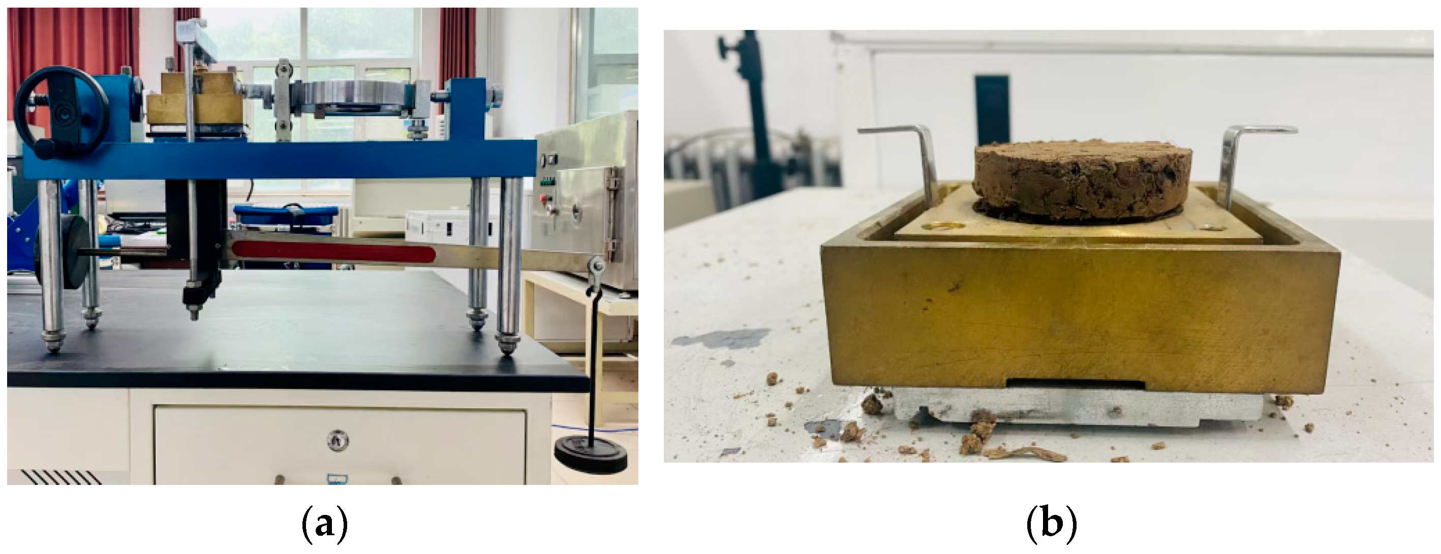
Agriculture 15 00129 g001
Figure 2. Direct shear test on soil. (a) ZJ-1B strain-controlled direct shear instrument; (b) test soil sample.
Agriculture 15 00129 g002
Figure 3. Curves of soil shear stress and shear displacement.
Agriculture 15 00129 g003
Figure 4. Mohr–Coulomb strength envelope diagram.
Agriculture 15 00129 g004
Figure 5. Test of wheat crop residue density.
Agriculture 15 00129 g005
Figure 6. Test for determining the soil static friction coefficient. (a) Test bench for the determination of the static friction factor; (b) Schematic diagram of static friction factor measurement test. 1. High-precision universal level; 2. test sample; 3. test sample container; 4. substrate; 5. handle adjustment.
Agriculture 15 00129 g006
Figure 7. Schematic diagram of rolling friction factor measurement test.
Agriculture 15 00129 g007
Figure 8. Collision recovery coefficient measurement test. (a) Test bench for determination of collision recovery coefficient; (b) Schematic diagram of collision recovery coefficient measurement.
Agriculture 15 00129 g008
Figure 9. Measurement principle of angle of repose.
Agriculture 15 00129 g009
Figure 10. Response surface diagram of the interaction between parameters that affect the angle of repose. (a) Response surface diagram of the interaction of X1 and X4 factors on the angle of repose. (b) Response surface diagram of the interaction of X1 and X7 factors on the angle of repose. (c) Response surface diagram of interaction between X1 and X10 factors on angle of repose. (d) Response surface diagram of the interaction of X4 and X7 factors on the angle of repose. (e) Response surface diagram of the interaction of X4 and X10 factors with respect to the angle of repose. (f) Response surface diagram of X7 and X10 factors interacting with the angle of repose.
Agriculture 15 00129 g010aAgriculture 15 00129 g010b
Figure 11. Soil angle of repose test. (a) Field test; (b) simulation test.
Agriculture 15 00129 g011
Figure 12. Particle bed for simulation test.
Agriculture 15 00129 g012
Figure 13. Surface roughness simulation cross-section.
Agriculture 15 00129 g013
Figure 14. Simulation cross-section of wheat crop residue coverage. (a) Particle bed surface after simulation; (b) grain distribution of wheat crop residues after soil particles were hidden.
Agriculture 15 00129 g014
Figure 15. Field trial.
Agriculture 15 00129 g015
Table 1. Measurement results of soil density and moisture content.
Test NumberSoil Density (kg/m3)Soil Moisture Content/%
12.23 × 10325.31
22.19 × 10321.85
32.13 × 10319.78
42.17 × 10321.47
52.20 × 10320.56
Mean value2.18 × 10321.79
Table 2. Soil particle size distribution.
Particle Size/mmAverage Mass/gPercentage/%
0~0.2558.4011.68
0.25~0.59.101.82
0.5~182.2516.45
1~225.205.04
2~3115.3023.06
>3209.7541.95
Table 3. Measurement results of wheat crop residue density.
Test NumberWheat Crop Residue Density (kg/m3)
1239
2243
3245
4236
5242
Mean value241
Table 4. Results of static friction factor measurement.
ContactStatic Friction Factor
Soil–65Mn steel0.57–0.91
Soil–soil0.25–0.85
Wheat crop residues–65Mn steel0.62–0.85
Soil–wheat crop residues0.60–0.80
Wheat crop residues–wheat crop residues0.20–1.16
Table 5. Test results of rolling friction factor.
ContactRolling Friction Factor
Soil–65Mn steel0.19–0.57
Soil–soil0.05–0.25
Wheat crop residues–65Mn steel0.30–0.62
Soil–wheat crop residues0.05–0.10
Wheat crop residues–wheat crop residues0.05–0.15
Table 6. Results of collision recovery coefficient measurement.
ContactCollision Recovery Coefficient
Soil–65Mn steel0.16–0.41
Soil–soil0.15–0.65
Wheat crop residues–65Mn steel0.21–0.35
Soil–wheat crop residues0.15–0.75
Wheat crop residues–wheat crop residues0.20–0.70
Table 7. Experimental results of the angle of repose for soil–wheat crop residues.
Test NumberAngle of Repose β/(°)
136.80
234.22
335.35
434.91
534.32
Mean value35.12
Table 8. Plackett–Burman test parameters of soil–wheat crop residue mix.
ArgumentParameter NameLevel
−1+1
X1Soil–soil collision recovery coefficient0.150.65
X2Soil–static friction factor of soil0.250.85
X3Soil–soil rolling friction factor0.050.25
X4Soil–wheat crop residue collision recovery coefficient0.150.75
X5Soil–wheat static friction factor of previous crop0.600.80
X6Soil–wheat crop residue rolling friction factor0.050.10
X7Coefficient of restitution for wheat stubble–wheat stubble collision0.200.70
X8Wheat crop residue–static friction factor of wheat crop residues0.201.16
X9Wheat crop residue–wheat crop residue rolling friction factor0.050.15
X10Soil surface energy (J·m−2)28
X11Virtual parameter--
Table 9. Plackett–Burman test scheme and results of soil–wheat crop residue mix.
IDX1X2X3X4X5X6X7X8X9X10Angle of Repose/(°)
10.150.850.250.150.80.10.70.20.05236.2
20.650.250.250.750.60.10.71.160.05239.6
30.150.250.050.150.60.050.20.20.05230.5
40.150.250.050.750.60.10.70.20.15832.2
50.650.250.250.750.80.050.20.20.15234.5
60.150.850.250.750.60.050.21.160.05836.4
70.650.850.050.750.80.10.20.20.05836.2
80.650.850.250.150.60.050.70.20.15847.7
90.650.850.050.150.60.10.21.160.15238.8
100.150.850.050.750.80.050.71.160.15235.1
110.150.250.250.150.80.10.21.160.15837.5
120.40.550.150.450.70.0750.450.680.1527.5
130.650.250.050.150.80.050.71.160.05847.3
Table 10. Significance analysis of Plackett–Burman feature parameters.
Source of VarianceSum of SquaresDegrees of FreedomMean Square ValueFp
model302.171030.22251.810.0490
X1109.201109.20910.030.0211
X26.4516.4553.780.0863
X311.60111.6096.690.0645
X448.00148.00400.000.0318
X50.213310.21331.780.4097
X610.08110.0884.030.0692
X748.80148.80406.690.0315
X825.23125.23210.250.0438
X90.013310.01330.11110.7952
X1042.56142.56354.690.0338
Table 11. Test design and results of steepest climb.
Serial NumberX1X4X7X10Angle of Repose/(°)Relative Error/%
10.1500.750.2002.032.577.26
20.2750.600.3253.536.584.16
30.4000.450.4505.038.168.66
40.5250.300.5756.539.0511.19
50.6500.150.7008.039.7113.07
Table 12. Box–Behnken test parameters of soil–wheat crop residue mix.
LevelExperimental Factor
X1X4X7X10
−10.2120.5250.3003.00
00.2750.6000.3253.50
10.3380.6750.3504.00
Table 13. Box–Behnken scheme and results.
Serial NumberX1X4X7X10Angle of Repose/(°)
1−110036.11
2011035.46
3000035.01
40−10−135.52
5110036.45
6−100−135.76
701−1135.81
80−11034.89
9−101035.73
10000035.05
11011−135.46
12000135.06
13−1−10036.97
14000035.01
15010135.81
1601−1035.75
17−10−1036.01
1800−1−134.6
19100−135.79
20000035.33
21001−134.98
22−100136.18
230−10135.55
240−1−1035.82
25000133.76
2610−1035.67
271−10035.78
28101035.09
29000035.19
Table 14. Analysis of variance of Box–Behnken regression model.
Source of VarianceSum of SquaresDegree of FreedomMean SquareF-NumberP-Number
model10.17140.726134.06<0.0001
X10.710510.710533.33<0.0001
X40.021710.02171.020.3304
X71.1811.1855.27<0.0001
X100.000210.00020.00980.9227
X1X40.585210.585227.450.0001
X1X70.022510.02251.060.3217
X1X100.330610.330615.510.0015
X4X70.102410.10244.800.0458
X4X100.025610.02561.200.2916
X7X101.4611.4668.68<0.0001
X123.0213.02141.46<0.0001
X421.9811.9893.08<0.0001
X720.248310.248311.650.0042
X1020.074110.07413.480.0833
Residual error0.2984140.0213
Missing fit0.2204100.02201.130.4934
Pure error0.078140.0195
total10.4628
Table 15. Physical parameters of soil–wheat crop residue mixture simulation.
ArgumentSoilWheat Crop Residues
Poisson’s ratio0.320.39
Density (kg/m3)2.18 × 103241
Shear modulus (kPa)1.2 × 1065.52 × 106
Surface energy (J·m−2)3.94-
Table 16. Simulation test contact parameters of soil–wheat crop residue mixture.
ContactStatic Friction FactorRolling Friction FactorCollision Recovery Coefficient
Soil–65Mn steel0.740.380.285
Soil–soil0.550.150.237
Wheat crop residues–65Mn steel0.740.460.280
Soil–wheat crop residues0.70.080.311
Wheat crop residues–wheat crop residues0.680.100.575
Table 17. The statistical results of the simulation experiment on the straw mulching rate.
Test NumberCover Rate of Wheat Crop Residues/%
189.1
282.5
383.7
481.6
584.4
Mean value84.26
Table 18. Results of surface roughness test.
Test NumberStandard Deviation of Surface Roughness/cm
12.59
21.82
32.11
41.96
52.30
Mean value2.16
Table 19. Results of straw burying rate in field trials.
Test NumberCoverage Rate of Wheat Crop Residues/%
182.3
275.1
386.5
483.1
587.6
Mean value82.92
Disclaimer/Publisher’s Note: The statements, opinions and data contained in all publications are solely those of the individual author(s) and contributor(s) and not of MDPI and/or the editor(s). MDPI and/or the editor(s) disclaim responsibility for any injury to people or property resulting from any ideas, methods, instructions or products referred to in the content.

