Assessing the Influence of Temperature and Precipitation on the Yield and Losses of Key Highland Crops in Ecuador

Abstract

Food production systems in Ecuador’s high Andean region are pivotal for food security, rural livelihoods, and agrobiodiversity, yet they are increasingly exposed to climate stress. We assessed four representative crops (tree tomato, quinoa, potato, and maize) across three Andean zones (North, Center, South) in 2015–2022 using monthly NASA POWER (MERRA-2) climate fields. After confirming non-normality, Spearman correlations and multiple linear regressions with leave-one-year-out validation were applied to quantify the influence of maximum/minimum temperature and precipitation on cultivated and harvested area, production, sales, and loss categories. To place monthly signals in a process context, daily extreme-event diagnostics (ETCCDI-style) were also computed: heat days ($\mathrm{TX}90$), ≥5-day dry spells, and the annual maximum consecutive dry days (${\mathrm{CDD}}_{max}$). Models explained a wide range of variability across crops and zones (approx. $R^2\sim 0.55$–0.99), with quinoa showing the most consistent fits (several outcomes $R^2>0.90$). Extremes provide an eye-catching, actionable picture: the Southern zone concentrated dryness hazards, with 1–5 dry spells $\ge 5$ days per year and ${\mathrm{CDD}}_{max}$ up to ∼8 days, while heat-day frequency showed non-significant declines across zones in 2015–2022. Reanalysis frost days were virtually zero—consistent with under-detection of local valley frosts at coarse resolution—so frost risk was interpreted via monthly signals and reported losses. Overall, the results show precipitation-driven vulnerabilities in the South and support quinoa’s role as a resilient option under increasing climate stress, offering concrete guidance for water management and climate-smart planning in mountain agroecosystems.

1. Introduction

High Andean Agri-food Systems (HAFS; Spanish: Sistemas Agroalimentarios Altoandinos, SAS) in Ecuador, located above 2500 m.a.s.l. [1], represent strategic territories for food security, agroecological sovereignty, and preservation of agrobiodiversity [2,3]. These mountainous areas, characterized by rugged topography and steep altitudinal gradients, generate a wide range of microclimates that enable the cultivation of numerous agricultural species adapted to extreme conditions [4,5,6]. Among the main crops, corn, potato, tree tomato, and, quinoa stand out.

SASs embody a profound body of agroecological knowledge, developed over centuries by Indigenous peoples and peasant communities [7,8,9]. This expertise is reflected in traditional practices such as crop rotation and intercropping, the construction of agricultural terraces to prevent soil erosion, and water management through canals, reservoirs, and gravity-fed irrigation systems [7,8,10]. Additionally, the raising of pigs, chickens, llamas, sheep, and guinea pigs supplements both household diets and family economies. Recognized by the Food and Agriculture Organization (FAO) as Globally Important Agricultural Heritage Systems (GIAHS), these systems uniquely integrate biodiversity, culture, and sustainability [11,12,13].

However, climate change is increasingly disrupting the stability and functioning of these systems. Interannual variability in rainfall, rising mean temperatures, and intensification of extreme events such as prolonged droughts or early frosts are reducing agricultural productivity, heightening pressure on water resources, and undermining rural livelihoods [14,15,16]. Projections for the tropical Andes indicate a massive warming on the order of 4–5 °C by the end of the 21st century under high-emission scenarios, alongside shifting precipitation patterns, which would severely threaten water supplies and crop viability. Recent studies warn of significant losses of suitable areas for climate-sensitive crops such as maize, with reductions exceeding 50% by mid-century under pessimistic scenarios [16,17]. By contrast, certain native crops like quinoa exhibit greater ecological plasticity and tolerance to abiotic stress [18,19,20]. Quinoa is notably resilient to drought, soil salinity, and frost, and it can thrive in marginal soils under harsh climatic conditions—attributes that give it a comparative advantage as climates become more extreme [18,19,20].

In this setting, quinoa emerges as a key crop for enhancing food resilience in the Andes. Its adaptability to marginal soils, drought tolerance, and high nutritional value—characterized by elevated protein, amino acid, fiber, and mineral contents—have driven its international promotion, particularly since its designation as an emblematic crop during the International Year of Quinoa in 2013 [21,22,23]. In Ecuador, quinoa is traditionally cultivated in Indigenous communities of the Central and Southern Highlands, where it offers a viable alternative to the decline of other climate-sensitive crops [19,22]. Furthermore, its growing international demand has created opportunities to improve rural incomes and strengthen short, sustainable marketing circuits. Beyond its economic value, quinoa holds deep cultural significance in high Andean territories, embedded in ritual agricultural practices, seed systems, and local knowledge that guide sowing, harvesting, and conservation [24,25]. Its cultivation also aligns with agroecological principles, facilitating crop rotations with legumes and enhancing soil fertility, thereby contributing to more resilient and sustainable farming systems [23,26].

In this context, the present study examines the productive efficiency and climate vulnerability of Ecuador’s high Andean agri-food systems in the face of climate change, focusing on four crops: tree tomato, potato, corn, and quinoa. Recent assessments conducted in Tungurahua have modeled how climate scenarios for 2050 may impact productivity of tree tomato, corn, and potato by integrating water availability, temperature, and extreme event projections [27]. A systematic statistical analysis is conducted to identify potential trends or fit adjustments to simple and multiple linear regression models. Based on the regression outcomes, trends are identified regarding the influence of specific independent (climatic) variables on dependent (agro-productive) variables. Although the analysis encompasses four high Andean products, detailed results are presented for quinoa, given its growing nutritional, ecological, and commercial relevance, as well as its adaptive capacity under adverse climatic conditions. The eco-efficiency of smallholder quinoa production in Andean systems has been recently quantified using life-cycle assessment and data envelopment approaches, providing a framework for evaluating both environmental and production resilience [28]. Details for the other crops are provided as supplementary material in the Appendix A, Appendix B, Appendix C and Appendix D section.

This article is structured as follows: Section 2 outlines the methodology applied for data collection and statistical analysis. This section presents agricultural variables for the four high Andean products, alongside climatic variables from Ecuador’s highland region, are subdivided into three subzones. Section 3 provides a descriptive statistical analysis of climatic variables to contextualize the study conditions. Section 4 reports the correlation analysis results between dependent and independent variables, displayed using heatmaps as a visual resource. Section 5 describes the proposed approach, which involves generating linear regressions between agricultural and climatic variables. Using the $R^2$ values from these regressions, those with higher coefficients (greater than 0.5) are selected to develop multiple linear regressions, thereby quantitatively assessing the influence of independent variables on dependent variables and evaluating the feasibility of employing the resulting equations as predictive tools. Finally, Section 6 summarizes the key conclusions drawn from the findings.

2. Methodology

To assess the efficiency of SASs and their relationship with climate change, we propose a methodology that integrates verified data from national statistical databases with satellite-based climatic information, identifying the dependent and independent variables of the study. Subsequently, statistical tools are employed to determine correlations among related variables. The variables are detailed as follows:

• Dependent variables: Cultivated Area (C.A.), Harvested Area (H.A.), Production (P.), Sales (S.), Losses due to drought (L.Drought), losses due to frost (L.Frost), losses due to pests (L.Pests), losses due to diseases (L.Diseases), losses due to flooding (L.Flooding), total losses (T.L.), and losses due to other reasons (L.O.R.), denote non-climatic drivers of agricultural losses, including logistic disruptions, market failures, and theft, as classified by ESPAC [29].
• Independent variables: maximum temperature (MaxTemp), minimum temperature (MinTemp), precipitation, northern zone (ZN), central zone (ZC), and southern zone (ZS).

Finally, multiple linear regressions are generated to provide insights into the relationships among variables and the influence of each.

2.1. Trends and Losses of High Andean Crops in Ecuador (2015–2022)

For this study, data on cultivated area, harvested area, production, sales, and losses due to various causes were used for soft corn, potato, quinoa, and tree tomato crops in Ecuador, covering the period from 2015 to 2022. These data were obtained from official sources (National Institute of Statistics and Census) (https://www.ecuadorencifras.gob.ec/encuesta-de-superficie-y-produccion-agropecuaria-continua-2014/, (accessed on 4 May 2023)), specifically from the Continuous Agricultural Area and Production Survey (ESPAC) (https://www.ecuadorencifras.gob.ec/encuesta-superficie-produccion-agropecuaria-continua-2021/, (accessed on 4 May 2023)). Based on this information, tables were prepared detailing the year-by-year evolution of the crops, both in terms of production and in losses caused by different factors.

2.1.1. Corn Production Information

According to ESPAC reports (as shown in

Table 1. Cultivated area, harvested area, production, sales, and losses due to different causes for soft corn during the period of 2015–2022 in Ecuador.

Year	2015	2016	2017	2018	2019	2020	2021	2022
Cultivated area (ha)	126,461	80,249	89,890	74,961	67,620	74,017	75,877	57,309
Harvested area (ha)	107,993	68,313	81,851	66,989	63,258	69,131	69,123	50,376
Production (t)	138,647	99,257	120,028	117,641	135,599	142,336	127,631	83,852
Sales (t)	102,459	75,649	89,042	88,351	108,177	115,311	98,571	64,300
Total losses	18,468	11,936	8039	7972	4361	4887	6754	6932
Losses due to drought	8841	6568	2081	5501	2311	2195	1493	1369
Losses due to frost	1597	1035	1394	894	487	733	2257	2046
Losses due to pests	2970	2862	1705	1010	1200	1205	1832	1517
Losses due to diseases	388	351	208	70	159	123	120	144
Losses due to flooding	129	51	1308	66	43	163	380	1522
Losses due to other reasons	4543	1068	1343	431	162	468	672	335

), between 2015 and 2022, the cultivated area of soft corn in Ecuador decreased by 55%. In contrast, higher yields per unit area were observed, indicating more efficient production practices among farmers. Nevertheless, the yield of soft corn in Ecuador remains below that reported by Peru and Bolivia, at 9.37 tonnes per hectare (t/ha) and 4.07 t/ha, respectively (https://sipa.agricultura.gob.ec/index.php/situacionales-agricolas/situacional-maiz-suave, (accessed on 4 May 2023)).

Losses in cultivated area for corn are primarily associated with climatic factors—drought, frost, and flooding—which have caused damage to 34 thousand hectares of crops between 2015 and 2022 [30].

2.1.2. Potato Production Information

During the period from 2015 to 2022, the cultivated area of potato in Ecuador decreased by 39.48%, according to ESPAC data. Despite this reduction, yields per hectare increased, particularly in 2020 and 2022. It is noteworthy that the crop faces significant losses due to factors such as frost and pests, as detailed in

Table 2. Cultivated area, harvested area, production, sales, and losses due to different causes for soft potato during the period of 2015–2022 in Ecuador.

Year	2015	2016	2017	2018	2019	2020	2021	2022
Cultivated area (ha)	32,036	32,741	32,187	23,974	20,626	25,923	20,950	19,390
Harvested area (ha)	29,703	29,634	29,532	22,099	19,675	24,882	19,088	17,926
Production (t)	397,520	422,589	377,243	269,200	275,345	408,313	244,748	251,433
Sales (t)	341,849	378,853	343,764	239,609	253,706	374,009	219,550	232,513
Total losses	2333	3107	2655	1875	951	1041	1861	1464
Losses due to drought	977	773	932	690	141	98	124	151
Losses due to frost	387	621	858	582	156	375	936	810
Losses due to pests	441	1344	333	190	420	306	537	199
Losses due to diseases	183	253	104	245	218	61	83	117
Losses due to flooding	39	10	185	94	13	28	72	154
Losses due to other reasons	304	104	240	71	—	170	108	31

.

According to farmers’ statements, pest-related losses have been the most significant, especially in Cotopaxi and Chimborazo. Furthermore, Castillo et al. [31] report that in the provinces of Carchi, Imbabura, Pichincha, and Cotopaxi, total losses of potato plots were recorded between 2014 and 2018, associated with the “Punta Morada” disease.

Freezing damage caused by so-called “frost events” is also highly detrimental, as plants cease photosynthetic activity [32], and in many cases, the damage is irreversible. In 2019, no other reasons for potato losses were reported, whereas in other years analyzed, they were linked to the use of common (non-certified) seed and inadequate cultivation practices.

2.1.3. Tree Tomato Production Information

According to ESPAC data, between 2015 and 2018, the cultivated area of tree tomato remained at approximately 2000 hectares. However, during the 2019–2021 period, this figure declined, followed by an increase in 2022. Notably, in 2016, losses exceeded 1000 hectares, mainly due to the adverse effects of drought, frost, pests, and diseases, making it the year with the most severe nationwide damage to this crop, as shown in

Table 3. Cultivated area, harvested area, production, sales, and losses due to different causes for soft tree tomato during the period of 2015–2022 in Ecuador.

Year	2015	2016	2017	2018	2019	2020	2021	2022
Cultivated area (ha)	1982	2075	1952	2026	1685	1044	1009	1364
Harvested area (ha)	1982	2075	1952	2026	1685	1044	1009	1364
Production (t)	16,175	28,512	20,212	22,343	24,316	10,605	6742	18,031
Sales (t)	15,779	28,018	19,715	22,081	23,904	10,472	6350	17,750
Total losses	241	2360	187	149	135	41	137	66
Losses due to drought	30	118	22	22	—	—	—	—
Losses due to frost	6	428	6	1	1	—	7	—
Losses due to pests	54	425	66	26	16	9	109	36
Losses due to diseases	36	162	66	40	69	2	21	13
Losses due to flooding	—	28	12	—	—	—	—	13
Losses due to other reasons	116	1200	15	61	48	30	1	4

.

Tree tomato production is distributed throughout Ecuador’s inter-Andean region, with Tungurahua being the province with the largest cultivated area. The crop requires approximately 125 mm/month of precipitation for optimal growth; however, in 2016, average precipitation reached only 67.85 mm/month in Imbabura and 45.70 mm/month in Tungurahua, leading to severe drought damage [33].

As with potato cultivation, the primary phytosanitary issue currently affecting tree tomato—and the cause of substantial losses—is “Punta Morada”, caused by Candidatus Liberibacter solanacearum (CaLso) and transmitted by the vector Bactericera cockerelli. This disease leads to flower abortion, fruit malformation, and a reduction in the size of the fruits that do develop [34].

2.1.4. Quinoa Production Information

Quinoa cultivation in Ecuador, according to ESPAC data, has shown marked instability in recent years. In 2015, 7886 hectares were planted; however, this figure progressively declined to 5365 hectares in 2020. By 2022, the cultivated area had dropped even further, reaching only 885 hectares. As shown in

Table 4. Cultivated area, harvested area, production, sales, and losses due to different causes for soft quinoa during the period of 2015–2022 in Ecuador.

Year	2015	2016	2017	2018	2019	2020	2021	2022
Cultivated area (ha)	7886	2765	1424	2215	2957	5365	2940	885
Harvested area (ha)	7148	2214	882	2048	2559	5267	2390	837
Production (t)	12,707	3903	1286	2146	4505	4903	1482	884
Sales (t)	10,739	3559	1128	2039	2603	4538	875	765
Total losses	738	552	542	167	399	98	550	49
Losses due to drought	534	65	—	63	—	51	60	—
Losses due to frost	47	54	2	—	75	10	420	23
Losses due to pests	—	282	—	—	—	37	9	26
Losses due to diseases	—	—	14	—	—	—	—	—
Losses due to flooding	126	1	507	86	—	—	60	—
Losses due to other reasons	31	150	20	19	323	—	—	—

, the crop has faced severe setbacks due to drought, frost, and pest outbreaks in various years, which have been the primary drivers of its negative trend.

According to data reported by the Ministry of Agriculture and Livestock (MAG) [35], quinoa production is concentrated mainly in the provinces of Cotopaxi and Chimborazo, where the lack of irrigation water and prolonged dry seasons represent critical constraints [36].

2.2. Climate Information

Meteorological data were retrieved from the NASA POWER Project (https://power.larc.nasa.gov/data-access-viewer, (accessed on 4 May 2023)), which provides variables from the MERRA-2 atmospheric reanalysis produced by the Global Modeling and Assimilation Office (GMAO). POWER/MERRA-2 provides temporally averaged, two-dimensional monthly means. We used bias-corrected precipitation from M2TMNXLFO [37] and 2 m maximum and minimum air temperatures from M2TMNXSLV [38] (

Table 5. Climatic datasets and variables used (NASA POWER/MERRA-2). All variables are temporally averaged, two-dimensional monthly means.

Variable	POWER/MERRA-2	Source	Temporal Support	Notes/IDs/Citations
Precipitation (bias-corrected)	M2TMNXLFO	NASA POWER (GMAO MERRA-2)	Monthly mean	Bias-corrected precipitation; dataset ID M2TMNXLFO [37].
Maximum air temperature (2 m)	M2TMNXSLV	NASA POWER (GMAO MERRA-2)	Monthly mean	Single-level product; dataset ID M2TMNXSLV [38].
Minimum air temperature (2 m)	M2TMNXSLV	NASA POWER (GMAO MERRA-2)	Monthly mean	Single-level product; dataset ID M2TMNXSLV [38].

).

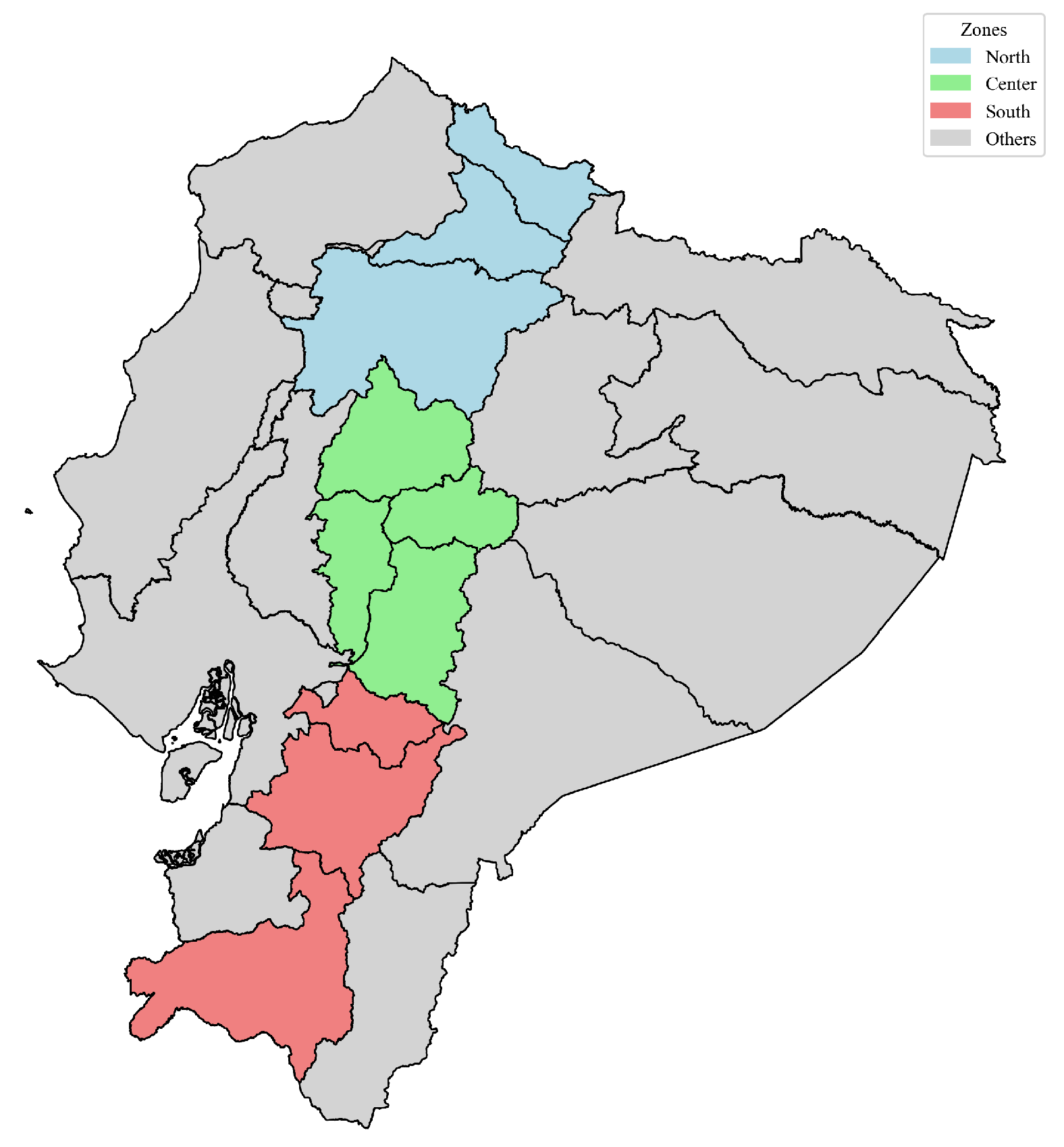
Given the strong environmental heterogeneity of the Andean cordillera, the Ecuadorian highlands were partitioned into three contiguous regions (North, Center, South) to reduce spatial confounding and provide zone-level controls in the models. This division is shown in Figure 1, and the details of the provinces that make up each region are shown in the table.

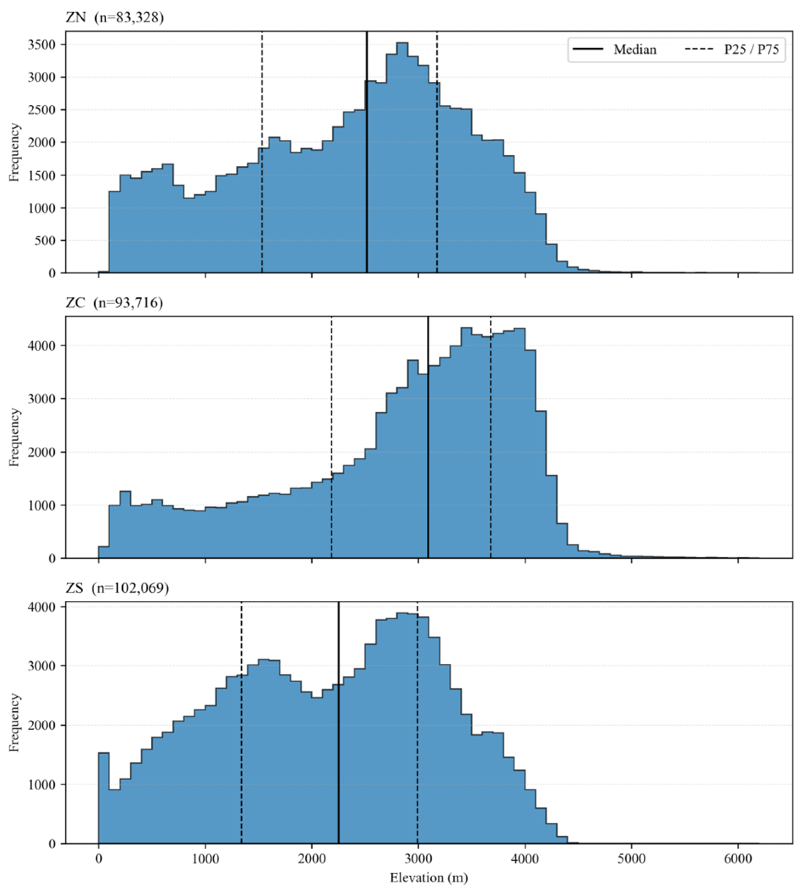
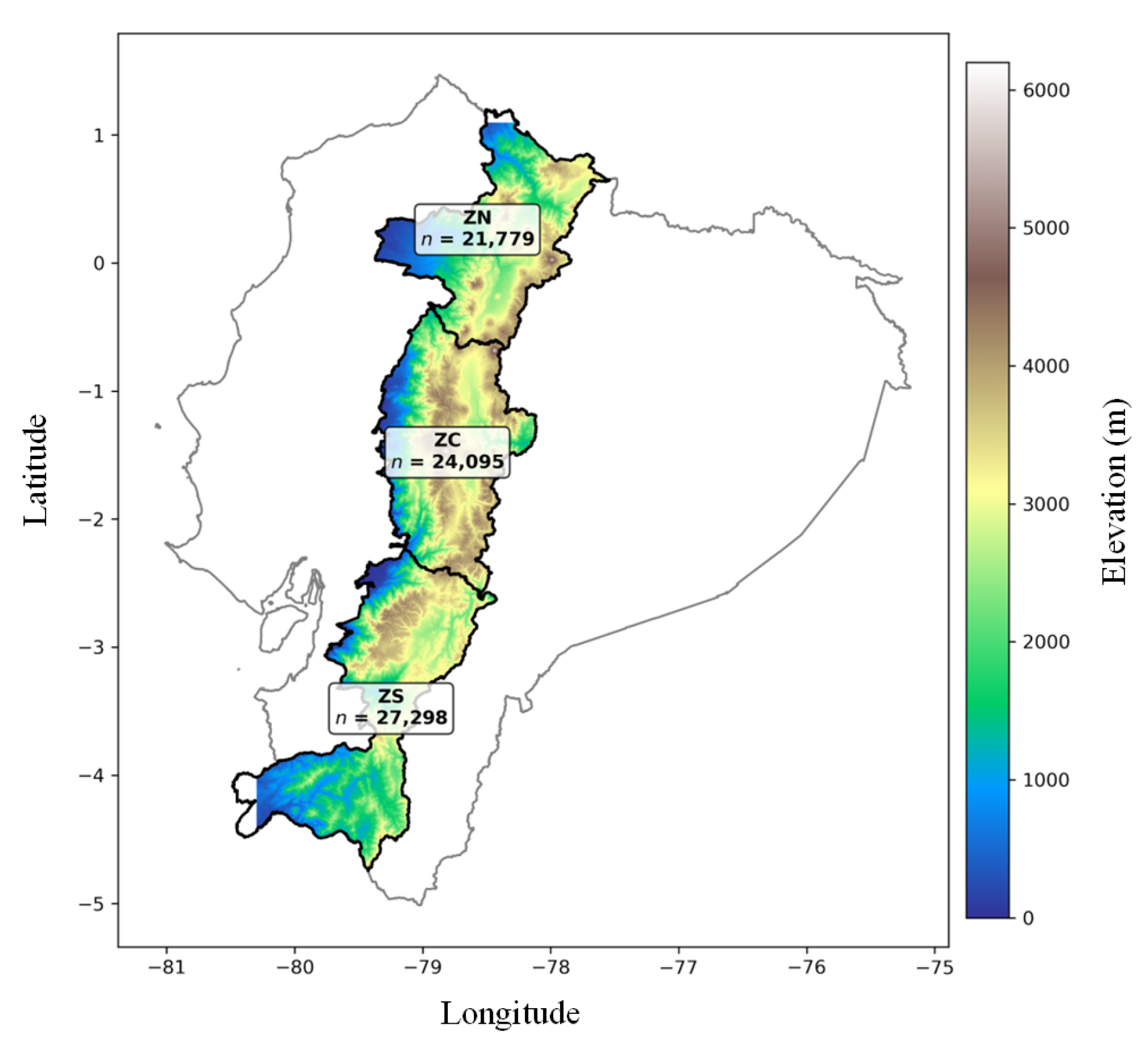
The regionalization follows continuous Andean provinces and is also compatible with administrative reporting units for agricultural statistics (

Table 6. Study area regionalization of the Ecuadorian highlands (N–C–S).

Region	Provinces
North (ZN)	Carchi, Imbabura, Pichincha.
Center (ZC)	Cotopaxi, Tungurahua, Chimborazo, Bolívar.
South (ZS)	Cañar, Azuay, Loja.

). To explicitly document intra-regional topographic variability, Figure 2 overlays the three zones on a SRTM15+ DEM; Supplementary Figure A1 shows altitude histograms (median and IQR) per zone; and

Table A1. Hypsometric summary by region based on SRTM15+ clipped to the Ecuadorian highlands.

Region	Min (m)	P25 (m)	Median (m)	P75 (m)	Max (m)	Mean (m)
ZN	90	1532	2520	3175	5654	2342
ZC	40	2188	3092	3678	6188	2823
ZS	15	1341	2254	2995	4429	2166

reports hypsometric summaries (min, P25, median, P75, max, mean).

Climate covariates were computed by spatially averaging all valid POWER/MERRA-2 grid cells intersecting each zone mask (all_touched=true) for every month in 2015–2022, then aggregating to the annual metrics used in the regressions. In this setup, the “sampling points” are the centroids of those intersecting grid cells.

Table 7. Sampling lattice and number of grid cells (“sampling points”) per region.

Grid (Product)	ZN	ZC	ZS	Definition/Note
MERRA-2 native (0.5° × 0.625°)	11	12	17	Sampling points are the centroids of all valid grid cells intersecting each region mask (all_touched=true); counts correspond to the spatial lattice used to extract monthly values (2015–2022).
POWER regridded (0.5° × 0.5°)	15	16	18	Same definition; shown for completeness given the 0.5° POWER grid commonly used in applications.

reports the number of sampling points per region using the native MERRA-2 grid (0.5° × 0.625°) and the commonly used POWER 0.5° × 0.5° lattice. For visual reference, Figure 2 also labels the count of a 1 km fishnet that tessellates the three zones (this fishnet is used only for visualization; statistical analyses use the POWER/MERRA-2 grids).

2.2.1. Validation of POWER/MERRA-2 Against in Situ Stations

To assess the suitability of the reanalysis data used in our models, we validated POWER/MERRA-2 monthly series against in situ observations within the Andean highlands for 2015–2022. We queried stations available through the Meteostat interface (which aggregates national and GHCN records), retained those located inside the highlands mask (ZN, ZC, ZS) and with ≥80% monthly coverage, and paired each station with the colocated POWER/MERRA-2 series (T_max, T_min, precipitation). Station observations were aggregated to monthly means (temperatures) and monthly totals (precipitation). Figure 3 shows the point-by-point comparison;

Table 8. Validation of POWER/MERRA-2 against in situ stations (monthly, 2015–2022). Median skill by region. RMSE/bias in °C for temperature and mm/month for precipitation.

Variable	Region	n Stations	r (Median)	RMSE	Bias	KGE
Tmax	ZN	2	0.56	1.65	1.19	0.40
Tmax	ZC	1	0.63	1.65	−1.21	0.37
Tmax	ZS	2	0.39	2.19	1.32	0.27
Tmin	ZN	2	0.54	2.41	2.16	0.43
Tmin	ZC	1	0.55	1.30	−0.45	0.43
Tmin	ZS	2	0.29	1.57	0.74	0.23
Precip	ZN	2	0.48	73.89	40.11	0.16
Precip	ZC	1	0.23	125.61	71.05	−0.57
Precip	ZS	2	0.41	77.75	33.06	−0.28

reports median skill by region (Spearman’s r, RMSE, bias, KGE).

T_max displays a strong linear correspondence with small, mostly additive, zone-dependent biases (slightly warm in the south and cool in the central zone). T_min also agrees well, with a modest cold bias in the northern/central zones. Monthly precipitation shows larger dispersion, with a typical drizzle bias in dry months and underestimation during wet months. Overall, the validation indicates that POWER/MERRA-2 provides reliable temperature covariates at the monthly scale and acceptable precipitation coherence for regional analyses (see Table 8 for exact metrics).

This validation is presented to demonstrate the adequacy of the climate inputs. As a robustness note, the observed temperature biases are mainly additive (offset), and precipitation errors are largely multiplicative; applying simple climatological bias corrections does not change the sign or statistical significance of our coefficients.

2.2.2. Scope of Climate Covariates and Control for Unobserved Factors

Our objective is to estimate first-order associations between climate and agro-production outcomes using covariates that are complete and comparable across all zones and years (2015–2022). We therefore restrict the climate inputs to three widely available POWER/MERRA-2 exposures: precipitation (P) and 2 m air temperatures ($T_{max},T_{min}$). This triad summarizes the dominant physical axes (water and energy) while avoiding comparability issues that would arise from adding covariates with spatial/temporal gaps (e.g., radiation, wind, relative humidity, irrigation or inputs), which lack homogeneous coverage by province and year in our study area.

To mitigate omitted-variable bias without altering the core dataset, we rely on a design with the following elements:

• Zone and year fixed effects: The econometric models include zone fixed effects (ZN, ZC, ZS) and year fixed effects, which absorb, respectively, time-invariant geographic heterogeneity (typical soils, mean elevation, persistent production systems) and year-specific national shocks (ENSO, macro events, prices). Thus, climate coefficients are identified from within-zone interannual variation.
• Topographic and microclimatic characterization: We explicitly document intra-regional heterogeneity by overlaying the three regions on a SRTM15+ DEM (Figure 2) and presenting hypsometric histograms by zone (Figure A1), with summary statistics (Table A1). These materials show that the regions are not topographically homogeneous and justify the inclusion of zone fixed effects.
• Sampling lattice and spatial support: We clarify that the “sampling points” used to compute zonal climate are the centroids of all valid POWER/MERRA-2 grid cells whose area intersects each regional mask (“all touched” convention). Per-region counts are as follows: native MERRA-2 grid (0.5° × 0.625°): ZN = 11, ZC = 12, ZS = 17; POWER 0.5° × 0.5° (regridded, reported for completeness): ZN = 15, ZC = 16, ZS = 18. The shapefile of zones and the CSV of grid-cell centroids are provided as Appendix A.
• External validation of the climate series: We validated monthly $T_{max}$, $T_{min}$, and P from POWER/MERRA-2 against in situ observations (via Meteostat) at stations within the highlands (2015–2022). Scatterplots are shown in Figure 3, and per-region median skill (Spearman’s r, RMSE, bias, KGE) is reported in Table 8. Temperatures show strong correspondence with small, mostly additive biases; precipitation exhibits larger dispersion with drizzle bias in dry months and underestimation in wet months, consistent with regional-scale use. These results support the suitability of the POWER/MERRA-2 series as zone-level climate exposures.
• Statistical handling consistent with the data: Given the non-normality of precipitation, descriptive analysis and nonparametric correlations (Spearman) are reported where appropriate. Climate regressors are centered and standardized (zero mean, unit variance) to facilitate interpretation and reduce scaling issues; multicollinearity was examined using variance-inflation factors (VIF) on standardized variables and found not to be problematic.

This deliberately parsimonious yet robust choice of covariates, together with fixed effects and explicit documentation of topographic structure and sampling support, controls in practice for a broad set of unobserved factors without introducing additional, heterogeneous, or potentially endogenous covariates (e.g., management or irrigation reacting to climate), which could induce post-treatment bias. Accordingly, we interpret coefficients as associations conditional on the specified controls rather than structural causal effects. The figures and tables (Figure 2, Figure 3 and Figure A1; Table A1 and Table 8) document the spatial structure and the validity of the climate series used, addressing the reviewers’ recommendation while keeping unchanged the data and the main analytical process.

2.2.3. Climate Information for the Northern Region

Climatic data for the northern region of the country are presented in

Table 9. Maximum temperature, minimum temperature, and precipitation values for the northern region.

Variable	Year	Jan	Feb	Mar	Apr	May	Jun	Jul	Aug	Sep	Oct	Nov	Dec	Mean
Maximum temperature (°C)	2015	24.92	24.45	25.17	24.57	24.73	24.79	25.28	26.05	26.52	26.10	25.57	26.56	25.39
	2016	25.90	26.10	25.59	25.46	25.38	24.42	24.66	26.28	25.67	25.40	24.40	23.39	25.22
	2017	24.10	24.21	23.50	24.01	23.80	23.74	23.75	24.16	24.54	25.36	22.91	23.57	23.97
	2018	23.25	23.60	24.17	24.19	23.91	23.95	23.95	24.40	25.18	24.49	24.24	24.17	24.12
	2019	25.07	24.01	25.13	24.52	24.43	24.65	24.34	25.29	25.68	24.02	24.08	24.34	24.63
	2020	25.12	24.92	24.23	24.33	24.76	23.96	24.31	25.63	25.60	26.05	24.76	23.62	24.77
	2021	24.30	23.77	23.80	23.13	24.00	23.64	24.03	24.50	24.75	25.22	23.25	23.46	23.99
	2022	23.85	22.22	22.25	23.47	24.02	22.54	23.61	24.18	24.52	24.37	23.55	23.33	23.49
Minimum temperature (°C)	2015	10.55	11.07	11.61	11.28	11.04	9.78	10.00	9.87	9.82	11.04	9.89	10.39	10.53
	2016	11.38	11.50	12.10	11.27	11.68	9.70	9.67	8.83	10.02	9.84	10.86	11.03	10.66
	2017	9.84	11.63	11.77	11.56	10.64	10.37	8.87	8.44	9.27	11.29	11.06	10.53	10.44
	2018	10.59	11.06	10.98	11.04	10.89	9.23	9.35	9.06	8.78	10.61	11.29	9.66	10.21
	2019	10.58	11.40	11.74	11.83	10.86	10.49	9.37	9.03	10.16	10.72	11.30	11.33	10.73
	2020	9.69	10.15	11.27	10.73	11.03	10.04	9.33	8.89	10.14	10.51	9.44	11.54	10.23
	2021	9.99	12.01	11.22	11.38	10.71	9.66	8.22	8.79	9.44	10.94	10.52	11.15	10.34
	2022	9.94	10.73	11.51	10.46	10.16	9.10	9.37	8.70	9.08	9.24	10.54	9.99	9.90
Precipitation (mm/day)	2015	14.36	13.38	13.55	13.30	13.69	15.01	15.29	16.18	16.71	15.06	15.68	16.16	14.86
	2016	14.53	14.60	13.49	14.19	13.70	14.73	14.99	17.44	15.65	15.56	13.53	12.36	14.56
	2017	14.26	12.58	11.73	12.45	13.16	13.36	14.89	15.72	15.27	14.07	11.86	13.04	13.53
	2018	12.66	12.54	13.18	13.16	13.02	14.71	14.59	15.34	16.39	13.88	12.94	14.51	13.91
	2019	14.49	12.61	13.38	12.69	13.56	14.17	14.98	16.26	15.52	13.30	12.79	13.01	13.90
	2020	15.43	14.76	12.97	13.61	13.73	13.92	14.98	16.73	15.46	15.54	15.32	12.08	14.54
	2021	14.31	11.76	12.59	11.75	13.29	13.98	15.80	15.71	15.31	14.28	12.73	12.31	13.65
	2022	13.91	11.48	10.73	13.01	13.86	13.44	14.25	15.48	15.44	15.12	13.00	13.34	13.59

. Average maximum temperature remains relatively stable throughout the year, with values around 26 °C. A slight increase is observed from January to May, reaching a peak in April and May. Subsequently, temperatures remain elevated during the summer months and decline slightly towards the end of the year.

Minimum temperature exhibits a more pronounced seasonal variation. It starts at approximately 10 °C in January, rises modestly to about 12 °C by April, and then decreases again towards year’s end. Summer months (June, July, August) record the lowest minimum temperatures, with August marking the lowest point.

Precipitation shows substantial variation over the annual cycle. March and April register the highest levels, close to 5 mm. Summer months display minimal precipitation, generally below 1 mm. An increase is recorded again in October and November, ranging from 2 mm to 4 mm.

Based on these data, Figure 4 presents a combined chart illustrating temperature and precipitation variations.

2.2.4. Climate Information for the Central Region

Climatic data for the central region of the country are presented in

Table 10. Maximum temperature, minimum temperature, and precipitation values for the central region.

Variable	Year	Jan	Feb	Mar	Apr	May	Jun	Jul	Aug	Sep	Oct	Nov	Dec	Mean
Maximum temperature (°C)	2015	22.35	21.45	21.40	21.11	21.07	20.67	21.63	22.16	23.65	23.34	23.15	23.26	22.10
	2016	22.94	22.03	22.32	21.61	21.47	20.60	20.89	22.79	22.53	22.89	23.20	22.03	22.11
	2017	22.10	20.63	20.08	20.74	20.32	20.50	21.43	21.90	22.23	22.95	22.01	22.29	21.43
	2018	21.39	21.53	21.15	20.92	21.09	21.18	20.82	21.52	22.81	22.23	22.68	21.65	21.58
	2019	22.11	21.08	20.96	21.46	21.13	20.86	21.49	22.05	23.09	22.17	22.50	22.29	21.76
	2020	23.15	22.18	21.77	21.45	22.30	21.41	21.15	22.99	23.46	23.65	23.63	21.72	22.40
	2021	20.54	20.71	20.52	20.55	21.14	20.75	20.86	21.69	22.33	22.96	21.91	22.08	21.34
	2022	22.25	20.36	20.61	20.66	21.00	20.11	20.80	22.13	22.80	23.39	22.40	22.30	21.57
Minimum temperature (°C)	2015	17.79	17.42	18.06	18.19	17.90	17.08	16.46	16.98	17.30	18.28	17.30	18.08	17.57
	2016	19.08	18.91	18.31	17.76	17.48	16.30	17.23	16.40	17.07	16.37	16.22	17.72	17.40
	2017	17.23	17.94	17.99	17.68	16.82	16.66	15.56	15.79	16.05	17.41	16.15	17.55	16.90
	2018	17.38	17.94	17.77	17.23	17.33	15.65	16.25	16.62	16.48	16.51	17.42	17.30	16.99
	2019	18.15	17.94	18.55	17.99	17.63	16.62	16.09	15.76	16.65	17.33	17.26	17.53	17.29
	2020	16.76	18.31	18.18	17.88	17.26	16.98	16.06	15.09	16.64	16.94	16.43	17.52	17.00
	2021	17.63	18.35	17.33	17.75	16.59	15.55	14.06	16.15	16.20	17.05	16.40	16.61	16.64
	2022	16.30	17.38	17.74	16.87	16.27	15.17	15.86	15.78	15.68	16.44	16.21	16.15	16.32
Precipitation (mm/day)	2015	15.54	13.48	12.73	11.97	12.00	13.87	16.67	17.27	17.66	17.09	15.83	16.41	15.04
	2016	13.66	11.30	11.61	11.98	13.20	15.98	15.41	19.16	17.36	16.90	16.56	14.46	14.80
	2017	14.98	10.84	10.55	11.36	11.80	12.32	14.91	16.77	16.98	17.23	15.34	14.45	13.96
	2018	13.32	13.05	11.98	13.01	12.74	16.42	16.52	17.40	18.37	15.62	14.66	14.48	14.80
	2019	13.55	11.20	10.45	10.62	11.84	14.01	16.34	18.63	18.42	15.55	15.14	15.47	14.27
	2020	16.96	12.01	11.05	11.55	14.70	14.83	16.65	19.20	16.48	17.39	15.72	13.34	14.99
	2021	10.92	9.90	11.06	10.80	12.87	13.99	17.59	16.45	17.64	16.11	14.46	14.34	13.84
	2022	15.51	10.55	9.34	12.36	13.09	14.50	15.93	17.27	18.45	18.10	15.96	15.53	14.72

. Average maximum temperature remains relatively stable, ranging from 17 °C to 20 °C. A slight increase is observed from May through September, peaking in September before declining modestly towards the year’s end.

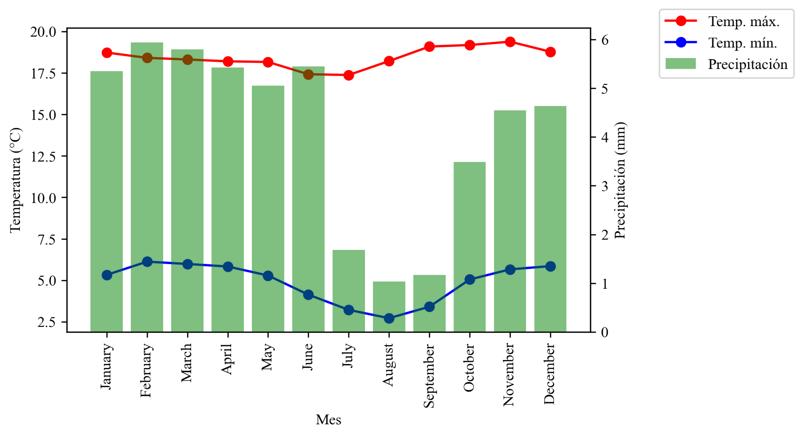
Average minimum temperature exhibits seasonal fluctuations. It starts at approximately 5 °C in January and remains relatively low during the first half of the year. In the summer months (June, July, August), minimum temperature decreases further, reaching its lowest point in July. From September onward, it shows a gradual increase.

Precipitation also displays marked variation throughout the year. The highest values occur in January, March, April, and December, ranging from 5 mm to 6 mm. Summer months register the lowest precipitation levels, generally below 1 mm. From September, rainfall increases, reaching a secondary peak in October and November.

Using these data, a combined temperature–precipitation chart was generated for the annual cycle, as shown in Figure 5.

2.2.5. Climate Information for the Southern Region

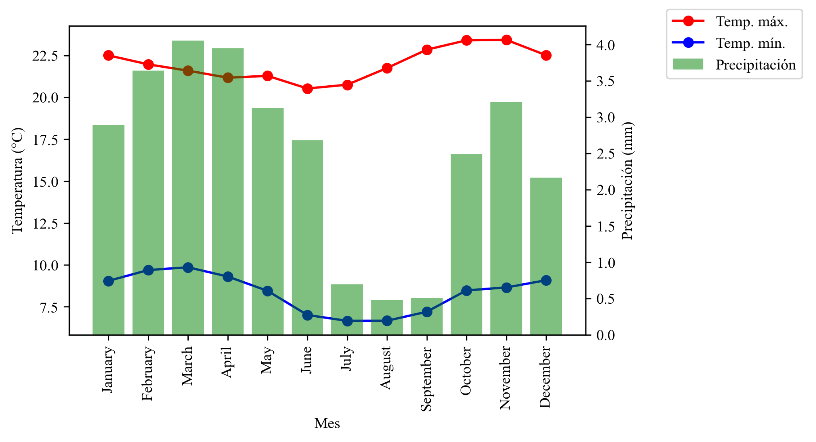
Climatic data for the southern region of the country are presented in

Table 11. Maximum temperature, minimum temperature, and precipitation values for the southern region.

Variable	Year	Jan	Feb	Mar	Apr	May	Jun	Jul	Aug	Sep	Oct	Nov	Dec	Mean
Maximum temperature (°C)	2015	24.01	23.46	23.37	22.15	22.32	22.27	23.51	24.06	25.67	24.85	25.12	25.45	23.85
	2016	25.61	24.56	24.31	23.20	23.36	21.93	22.44	24.20	24.61	25.09	25.61	23.56	24.04
	2017	23.41	22.32	21.80	22.00	21.38	21.93	22.57	23.40	24.39	24.61	24.32	24.13	23.02
	2018	23.79	23.16	23.35	22.81	23.17	22.85	22.77	23.13	24.39	24.42	24.10	23.20	23.43
	2019	24.29	22.98	23.00	23.06	23.46	22.83	23.51	23.42	24.62	23.56	24.20	23.76	23.56
	2020	24.47	24.04	23.24	22.98	23.70	23.27	22.38	24.36	24.85	25.41	25.46	23.37	23.96
	2021	22.98	23.39	21.81	22.29	22.86	22.42	22.44	23.57	24.34	25.37	23.40	23.76	23.22
	2022	23.36	22.38	22.02	22.20	22.38	21.77	22.39	23.38	24.68	25.61	24.66	24.67	23.29
Minimum temperature (°C)	2015	10.28	10.34	10.96	10.60	9.58	9.10	8.44	8.77	8.05	10.32	9.57	9.40	9.62
	2016	11.07	11.19	11.85	10.69	9.17	8.82	8.16	7.49	8.81	8.32	8.52	9.90	9.50
	2017	10.11	9.64	10.64	10.51	9.18	8.10	6.83	7.69	8.60	9.61	8.86	10.13	9.16
	2018	9.80	10.40	10.50	10.31	9.73	6.59	7.73	8.07	6.13	9.72	10.85	9.51	9.11
	2019	10.12	11.58	10.71	11.07	10.01	8.22	7.82	7.47	8.76	9.75	9.24	10.58	9.61
	2020	10.17	10.30	10.65	8.77	10.30	8.42	8.46	8.40	9.28	8.89	9.14	10.79	9.47
	2021	9.82	10.69	10.21	10.36	9.44	8.72	7.27	7.86	8.33	10.24	9.69	10.34	9.41
	2022	9.20	10.44	10.29	9.82	8.52	6.63	8.17	7.06	8.20	8.95	9.59	9.22	8.84
Precipitation (mm/day)	2015	12.68	12.73	11.62	12.38	13.30	14.67	15.51	15.29	17.61	14.53	15.55	16.04	14.33
	2016	13.59	12.22	12.14	14.14	13.20	14.41	17.24	16.71	15.80	16.77	17.09	13.66	14.75
	2017	11.98	10.52	10.92	11.47	12.91	14.98	15.44	15.71	15.79	15.00	15.46	14.01	13.68
	2018	12.52	13.31	12.43	13.75	16.22	16.02	15.36	15.07	18.26	14.70	13.25	13.69	14.55
	2019	11.13	11.81	11.86	13.41	15.06	15.48	16.09	15.95	15.86	13.81	14.96	13.18	14.05
	2020	13.89	12.66	13.58	12.95	14.85	14.31	16.60	15.96	15.57	16.52	16.31	12.58	14.65
	2021	12.60	10.73	11.80	13.59	13.85	15.85	14.72	15.72	16.01	15.14	13.71	13.42	13.93
	2022	10.65	10.09	12.58	13.55	15.04	14.73	16.57	16.32	16.49	16.66	15.07	15.45	14.43

. Average maximum temperature shows slight variation throughout the year. It starts at approximately 22 °C in January, remains relatively steady until May, then increases gradually from June, peaking around September and October with values close to 24 °C. After October, maximum temperatures gradually decline towards the end of the year.

Average minimum temperature exhibits a more pronounced seasonal pattern. It begins at about 7.5 °C in January, rises slightly to around 9 °C in April, and then decreases to its lowest point in July and August, with values near 6 °C. From September onward, minimum temperature gradually increases again.

Precipitation varies considerably over the annual cycle. March and April record the highest values, around 4 mm. Summer months (June, July, August) register the lowest precipitation, with values below 1 mm. Rainfall rises again from October, reaching nearly 3 mm in November.

The combined temperature–precipitation chart for the southern region is shown in Figure 6.

2.3. Operational Early-Warning Thresholds

To provide operational value, we derived general early-warning thresholds per crop. Based on the strongest climate–yield associations detected in our regressions and heatmaps, we identified critical climatic ranges that consistently led to yield reductions or increased losses. For each crop, thresholds were defined in terms of high or low percentiles (≈P75, P90, P95) of monthly temperature or precipitation, corresponding to “yellow” (increased vigilance), “orange” (≈10% yield loss), and “red” (>10% loss) alert levels. These thresholds were then matched with the main phenological phases to suggest practical management actions.

Table 12. Proposed early-warning thresholds by crop, based on percentile ranges of critical climatic variables. Thresholds are general by crop and phenological stage, with suggested management actions.

Crop	Critical Phenology	Sensitive Variable	Yellow (≈P75)	Orange (≈P90)	Red (≈P95)	Main Risk	Recommended Action
Quinoa	Flowering–grain filling	Precipitation (excess)/Tmin (low)	≥P75 rain/≤P25 Tmin	≥P90 rain/≤P10 Tmin	≥P95 rain/Tmin extremes	Flooding, pests, frost	Drainage, row covers, adjust planting dates
Corn	Sowing–flowering	Precipitation (deficit/excess)/Tmax (high)	≤P25 (drought)/≥P75 (rain)	≤P10/≥P90	≤P5/≥P95	Drought, flooding, heat stress	Irrigation, drainage, staggered planting dates
Potato	Tuber initiation–bulking	Tmin (frost)/Precipitation (excess)	Tmin ≤ P25/P75 rain	Tmin ≤ P10/P90 rain	Tmin ≤ P5/P95 rain	Frost, fungal diseases	Anti-frost covers, fungicide application
Tree tomato	Flowering–fruiting	Precipitation (high)/Tmin (low)	≥P75 rain	≥P90 rain	≥P95 rain	Fungal diseases, flower abortion	Preventive fungicide, pruning, ventilation

summarizes the proposed thresholds by crop. For quinoa, excess rainfall during the rainy season and extreme temperature drops in reproductive stages were the main risk triggers. For corn, both drought and flooding extremes during establishment and flowering phases defined alert levels. For potato, frost events and excess rainfall during tuber initiation and bulking emerged as critical thresholds. For tree tomato, high rainfall during flowering and fruit set phases increased the probability of disease outbreaks. These thresholds provide general yet actionable rules to guide early-warning systems in the Andean highlands.

In all cases, we applied the same methodology uniformly, without any modifications between datasets or zones. This consistency ensures that observed differences in results arise from the data themselves and not from analytical inconsistencies. For example, both the NASA POWER (0.5° × 0.5°) and MERRA-2 (0.5° × 0.625°) climate data were processed with identical procedures (e.g., the same aggregation of grid cells per zone and the same trend or regression analyses). Maintaining a uniform approach across data sources is important for robust comparisons [39]. Other studies have successfully utilized reanalysis datasets like ERA-Interim or MERRA-2 for agricultural analyses without altering the methodology per region, emphasizing that a consistent framework can be applied even if the data have coarse resolution [40]. By not introducing case-specific adjustments, we avoid potential bias and follow best practices for multi-region climate analysis. This approach is further justified by literature showing that despite some limitations (e.g., reanalyses’ lower spatial resolution), these datasets can reliably be used for climate and agriculture studies when handled consistently [41].

3. Statistical Analysis of Climate Variables

A descriptive statistical analysis of the independent (climatic) variables was first conducted to identify trends or patterns potentially relevant for subsequent correlation assessments with the remaining variables. Although the combined charts already provide valuable insights, a more detailed exploration was performed using box-and-whisker plots, enabling the identification of additional information regarding value distributions and the months exhibiting the greatest variability.

3.1. Variations in Maximum Temperature Values

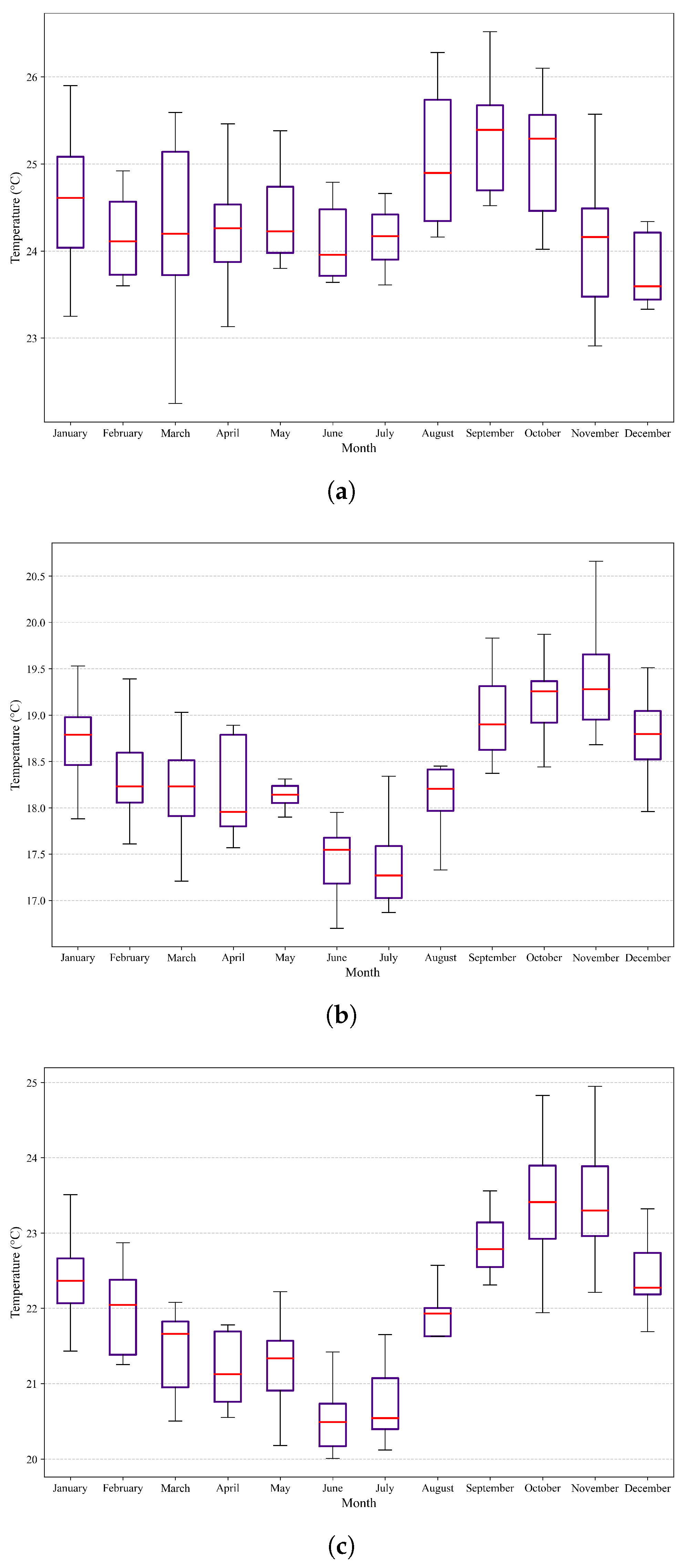
In the northern region (Figure 7a), maximum temperatures range from 15 °C to 20 °C throughout the year. The median shows a slight increase during the summer months (June to August) and a decrease during winter (December to February). Notable dispersion in maximum temperatures is observed, particularly in May and from September to November, suggesting greater climatic variability during these periods. Outliers are also recorded in January, March, and October, indicating the occurrence of unusual weather events. The region’s altitudinal diversity, encompassing both high Andean areas and lower-altitude zones, contributes to this variability in temperature.

The central region (Figure 7b) exhibits lower maximum temperatures, with median values ranging from 10 °C to 15 °C year-round. The narrower interquartile ranges in the boxplots indicate reduced variability compared to the northern region. Fewer outliers are observed, suggesting a more stable and predictable climate. The presence of high elevations and mountain ranges, including Chimborazo and Cotopaxi, plays a significant role in maintaining low and stable temperatures in this area.

In the southern region (Figure 7c), maximum temperatures range from 12 °C to 18 °C. A marked increase is observed towards the end of the year, particularly from October to December. Similar to the central region, variability is relatively low, as indicated by the narrower interquartile ranges in the boxplots. Nevertheless, some outliers are recorded, especially in June and December, pointing to the occurrence of extreme weather events. The region’s varied topography, encompassing both mountainous areas and valleys, influences these temperature variations.

Figure 7 compares the three regions. The northern region exhibits the greatest variability and the most outliers in maximum temperature, influenced by its altitudinal diversity. The central region presents lower maximum temperatures and fewer fluctuations, largely due to its high elevations. In contrast, the southern region, characterized by varied topography, shows a notable increase in maximum temperatures towards the year’s end and moderate variability overall. These findings highlight the role of geography and altitude in shaping maximum temperature patterns across different regions of Ecuador.

3.2. Variations in Minimum Temperature Values

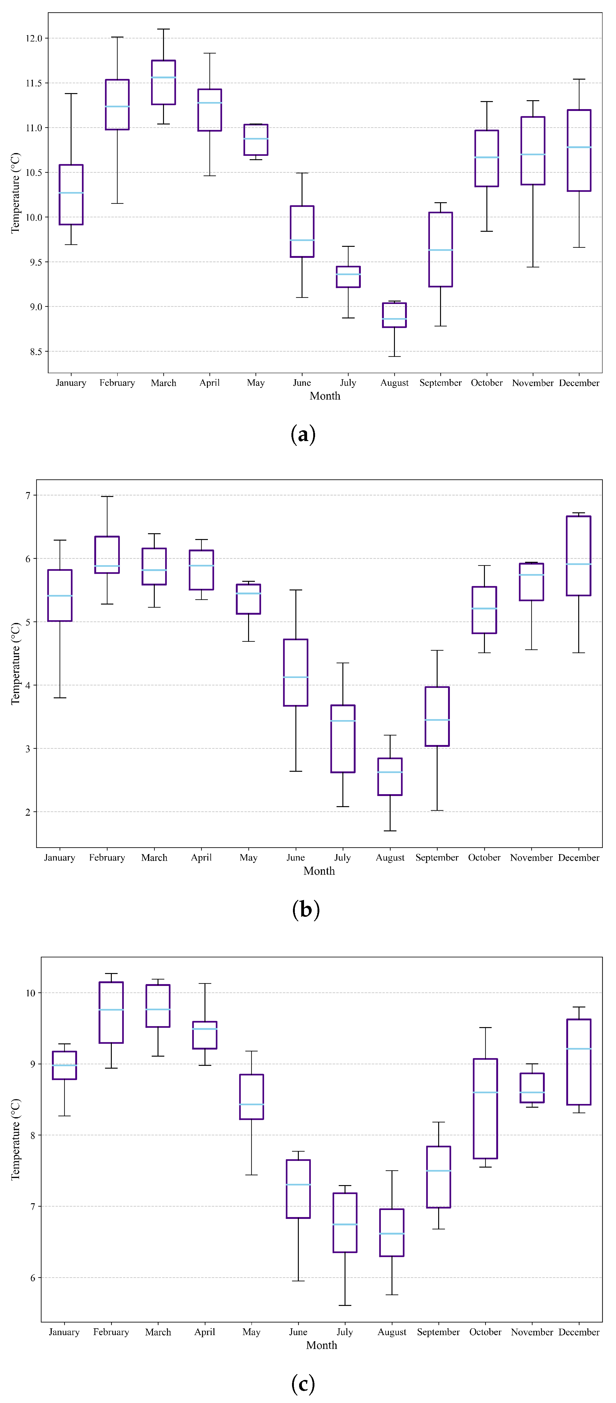
In the northern region (Figure 8a), minimum temperatures range from approximately 7 °C to 12 °C throughout the year. The median shows a slight increase during the summer months (June to August) and a decrease during winter (December to February). Considerable dispersion is observed in minimum temperatures, particularly in May and from September to November, suggesting greater climatic variability during these periods. Outliers recorded in January and October indicate the occurrence of unusual weather events. The altitudinal diversity of this region contributes to the observed variability in minimum temperatures.

The central region (Figure 8b) exhibits lower minimum temperatures, with median values ranging from 5 °C to 10 °C throughout the year. The relatively narrow interquartile ranges in the boxplots indicate reduced variability compared to the northern region. Fewer outliers are observed, suggesting a more stable and predictable climate. The presence of high elevations and mountain ranges, including Chimborazo and Cotopaxi, plays a significant role in maintaining low and stable temperatures in this area.

In the southern region of Ecuador (Figure 8c), encompassing the provinces of Cañar, Azuay, and Loja, minimum temperatures range from 5 °C to 10 °C. A marked increase is observed towards the end of the year, particularly from October to December. Similar to the central region, variability is relatively low, as reflected in the narrower boxplots. Nevertheless, some outliers are recorded, especially in June and December, pointing to the occurrence of extreme weather events. The region’s varied topography, including mountainous areas and valleys, influences these temperature variations.

Figure 8 compares the three regions. The northern region shows the greatest variability and the most outliers in minimum temperatures, influenced by its altitudinal diversity. The central region records lower minimum temperatures and fewer fluctuations due to its elevated terrain. In contrast, the southern region, characterized by varied topography, displays a notable increase in minimum temperatures towards year’s end and moderate variability. These findings underscore the influence of geography and altitude on minimum temperature patterns across Ecuador’s regions.

3.3. Variations in Precipitation Values

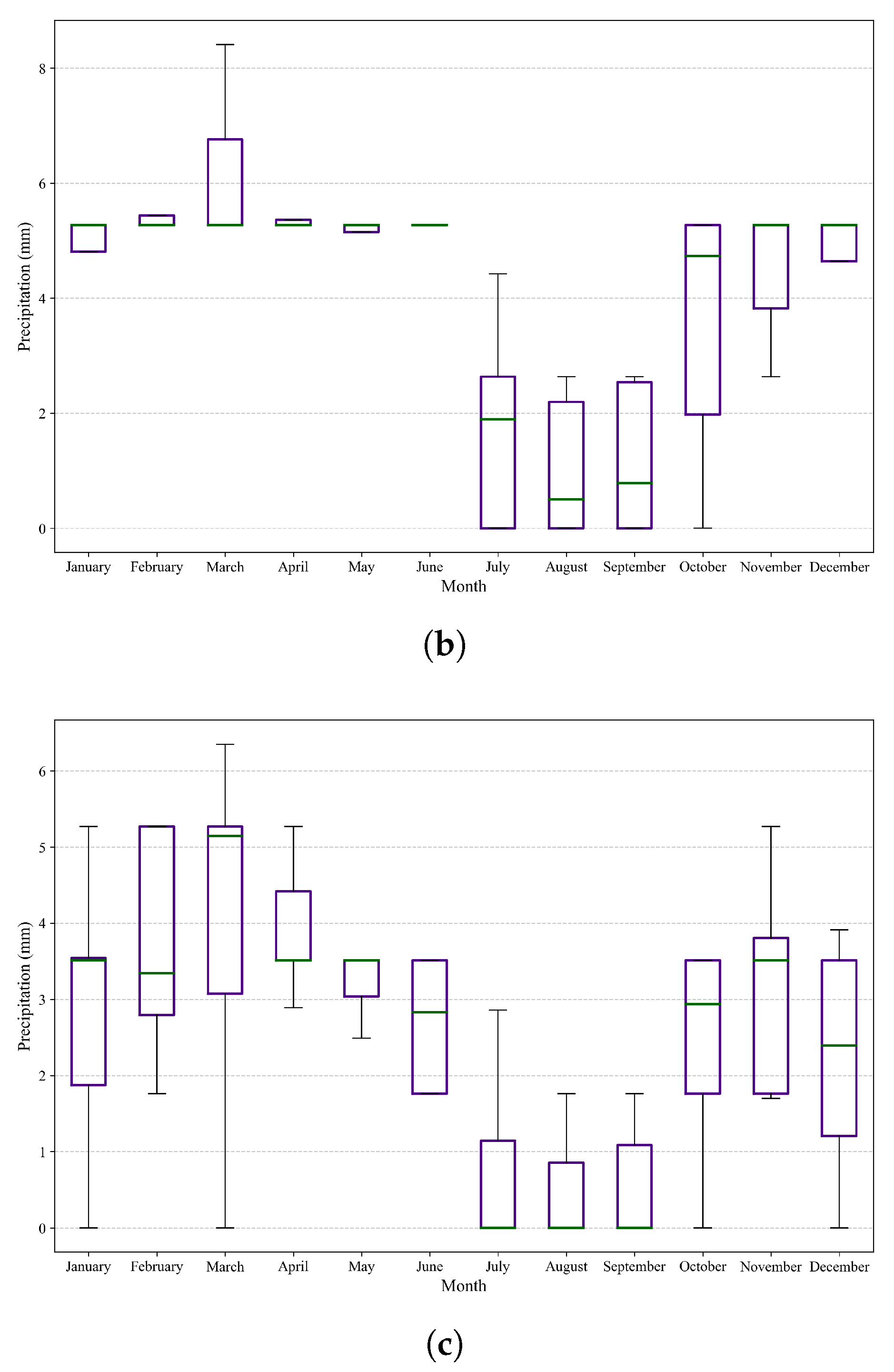
In the northern zone (Figure 9a), precipitation varies significantly throughout the year. The median precipitation values are higher from January to April and from October to December. The boxplots display wider boxes during these months, indicating greater variability in rainfall. Extreme values are observed in almost all months, particularly in January, March, and October, suggesting the occurrence of extreme weather events. The altitudinal diversity of this region, which includes both high Andean lands and lower areas, contributes to the variability in precipitation.

The central zone (Figure 9b) exhibits lower precipitation variability compared to the northern zone. The medians show higher values from January to May and from October to December, while the months from June to September register significantly lower precipitation. The boxplots are narrower during the dry season (June to September), indicating reduced variability. However, extreme values are observed, especially in March and October, suggesting the occurrence of unusual climatic events. The high altitudes of this region influence the distribution of precipitation.

In the southern zone (Figure 9c), precipitation shows greater variability during the winter months (December to April) and a notable decrease during the summer months (June to August). The boxplots display wider boxes from December to April, indicating higher variability in rainfall. Several extreme values are observed in January and March, suggesting the occurrence of extreme weather events. The varied topography of this region, which includes mountainous areas and valleys, influences these variations in precipitation.

When comparing the three zones (Figure 9), the northern zone exhibits the greatest variability and extreme precipitation values, influenced by its altitudinal diversity. The central zone has a more balanced precipitation distribution, with lower variability during the dry season and higher values during the rainy months, due to its elevated altitudes. In contrast, the southern zone shows marked seasonality, with higher precipitation and variability in the winter months and a decrease during summer, influenced by its varied topography. These observations reflect how geography and altitude affect precipitation across different regions of Ecuador.

4. Correlation Analysis Between Variables

Prior to conducting the correlation analysis among the study variables, it is essential to determine whether parametric or non-parametric statistical tests should be applied. Based on the visual inspection of the box-and-whisker plots presented in Section 2.2, the median appears non-centralized, and the whiskers show unequal lengths. This suggests that the data distribution may deviate from normality, implying the need for non-parametric tests. Nonetheless, to ensure this conclusion, a formal normality assessment through statistical testing is required.

4.1. Normality Analysis of Variables

Shapiro–Wilk (SW) and Anderson–Darling (AD) tests are applied to assess the normality of the data. These tests are performed on both the dependent and independent variables.

4.1.1. Production Variables for the Four Key Highland Crops

Table 13. Normality tests for production variables of the four key highland crops. Shapiro–Wilk test (p-value), Anderson–Darling statistic.

Crop	Variable	Result	Shapiro–Wilk (p)	Anderson–Darling	Notes
Corn	L.Flooding	Non-normal	0.0033	1.0882	Deviates in both tests
	L.O.R.	Non-normal	0.00088	1.1922	Deviates in both tests
	L.Drought	Marginal normality	0.0522	N/A	Close to threshold
	T.L.	Marginal normality	0.0590	N/A	Close to threshold
	C.A.	Marginal normality	0.0667	N/A	Close to threshold
Potato	L.Frost	Non-normal	0.0289	0.7350	Deviates in both tests
	L.Diseases	Non-normal	0.0035	0.9779	Deviates in both tests
	P.	Marginal normality	0.0545	N/A	Near 5% threshold
Tomato	L.Drought	Non-normal	<0.00001	1.9850	Strong deviation
	L.Frost	Non-normal	0.00079	1.1826	Deviates in both tests
	L.Pests	Non-normal	0.0000017	2.3017	Strong deviation
	L.Diseases	Non-normal	0.00032	1.3429	Deviates in both tests
	L.O.R.	Non-normal	0.00379	1.0514	Deviates in both tests
	T.L.	Non-normal	0.0000101	1.9479	Deviates in both tests
	L.Flooding	Marginal normality	0.0722	N/A	Close to threshold
Quinoa	P.	Non-normal	0.0129	0.7792	—
	S.	Non-normal	0.0135	0.7631	—
	L.Frost	Non-normal	0.0000558	1.6378	Strong deviation
	L.Pests	Non-normal	0.00013	1.4794	Strong deviation
	L.Diseases	Non-normal	0.0000251	1.7634	Strong deviation
	L.Flooding	Non-normal	0.0000115	1.9325	Strong deviation
	L.O.R.	Non-normal	0.0347	0.6522	—
	T.L.	Non-normal	0.00429	0.9853	—

reports the results of normality tests for the production variables of corn, potato, tomato, and quinoa. Both Shapiro–Wilk and Anderson–Darling statistics are presented, providing an assessment of the distributional assumptions required for further parametric analyses.

4.1.2. Normality Tests for Maximum Temperature

Table 14. Normality tests for maximum temperature. Shapiro–Wilk test (p-value), Anderson–Darling statistic.

Zone	Variable	Result	SW p	AD
North	December	Non-normal	0.00220	1.0447
	All others	Normal	>0.05	<0.709
Central	February	Marginal normality	0.0991	–
	April	Marginal normality	0.0602	–
	All others	Normal	>0.05	<0.709
South	April	Marginal normality	0.0776	–
South	All others	Normal	>0.05	<0.709

summarizes the outcomes of normality tests applied to maximum temperature data across the three regions. The results highlight months with deviations from normality, which are relevant for climate trend evaluation.

4.1.3. Normality Tests for Minimum Temperature

Table 15. Normality tests for minimum temperature. Shapiro–Wilk test (p-value), Anderson–Darling statistic.

Zone	Variable	Result	SW p	AD
North	All variables	Normal	>0.05	<0.709
Central	All variables	Normal	>0.05	<0.709
South	June	Non-normal	0.0354	0.7165
	Annual mean	Marginal	0.0543	–
	Others	Normal	>0.05	<0.709

presents the normality assessment of minimum temperature data for the northern, central, and southern regions. While most variables comply with normality, certain cases exhibit marginal or significant deviations.

4.1.4. Normality Tests for Precipitation

Table 16. Normality tests for precipitation. Shapiro–Wilk test (p-value), Anderson–Darling statistic.

Zone	Month/Variable	Result	SW p	AD
North	Jan, Mar, Apr, Jun, Jul, Aug, Sep, Oct	Non-normal	<0.05	Up to 2.1909
	Feb, May, Nov, Dec	Normal	>0.05	<0.709
Central	Jan, Feb, Apr, May, Jun, Aug, Sep, Oct, Nov, Dec	Non-normal	<0.05	Up to 1.7882
	Mar, Jul, Annual mean	Normal	>0.05	<0.709
South	Apr, May, Jun, Jul, Aug, Sep, Oct	Non-normal	<0.05	Up to 1.2214
	Jan, Feb, Mar, Nov, Dec, annual mean	Normal	>0.05	<0.709

displays the results of normality tests for monthly and annual precipitation values across regions. The findings reveal notable departures from normality in several months, particularly in the northern and central zones.

On the one hand, the results indicate that while some variables, such as cultivated area and losses due to drought, follow normal distributions, others, such as production and sales, do not exhibit normality. On the other hand, within the climate data matrices, only maximum temperature records in the northern zone during December show normality with adequate statistical significance.

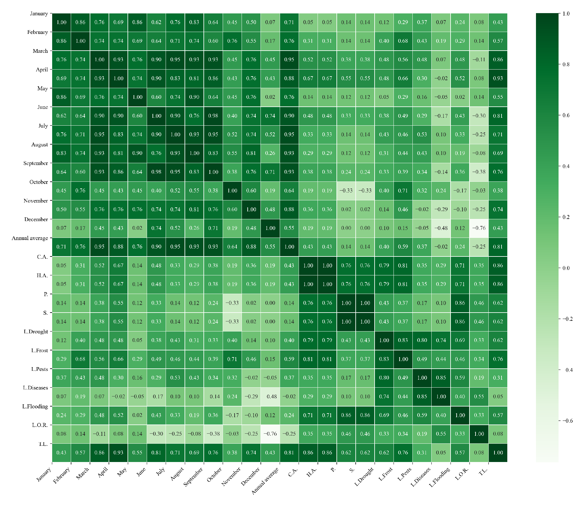
Given these results, non-parametric tests were applied to perform the statistical analysis, specifically the Spearman correlation. This analysis is crucial for understanding how climatic variations can influence agriculture and for developing adaptation and mitigation strategies in response to climate change. For conciseness, the detailed analysis is presented only for quinoa cultivation, while the results for corn, potato, and tree tomato are included in the appendices.

4.2. Correlation Analysis of Quinoa Variables

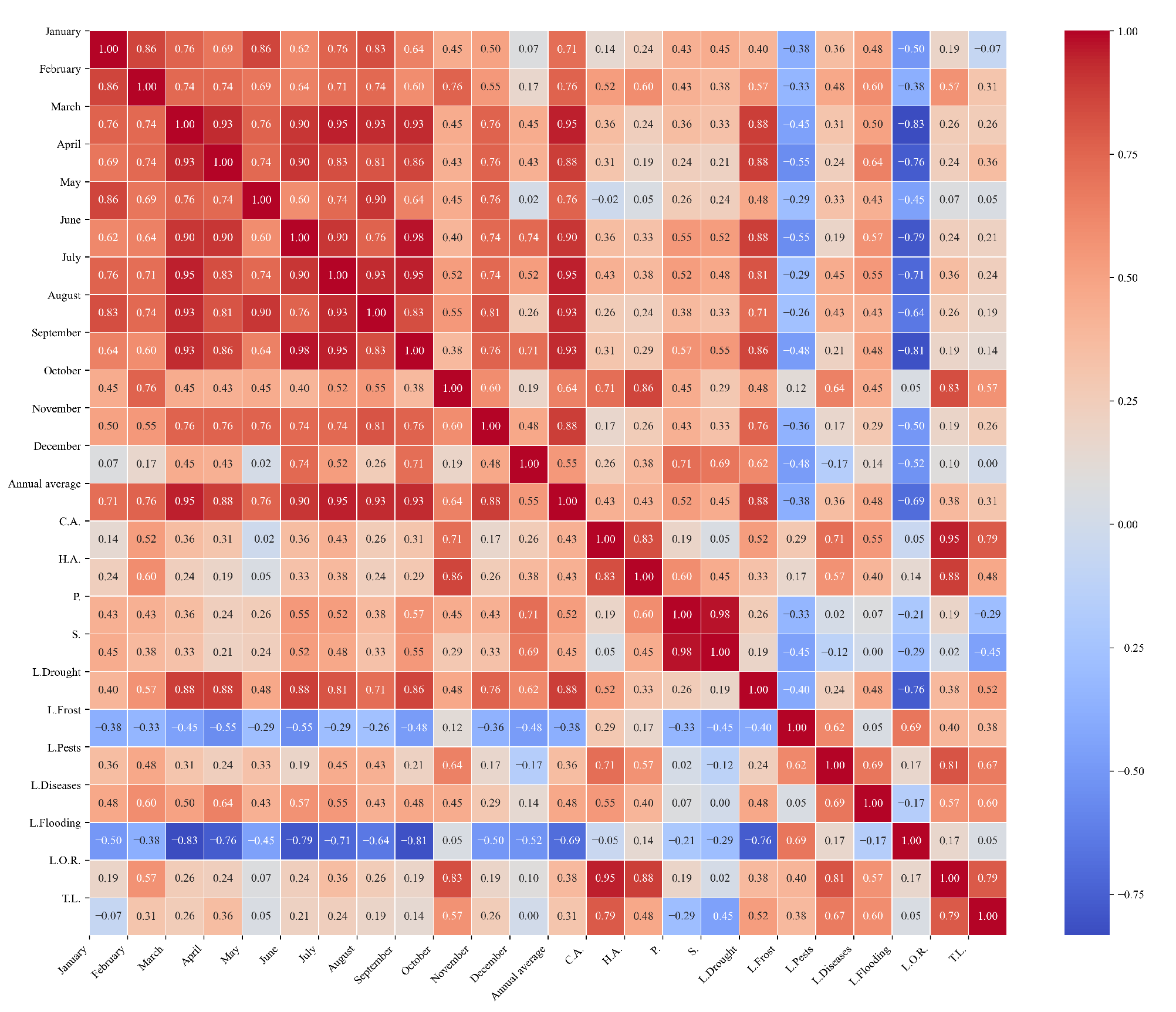
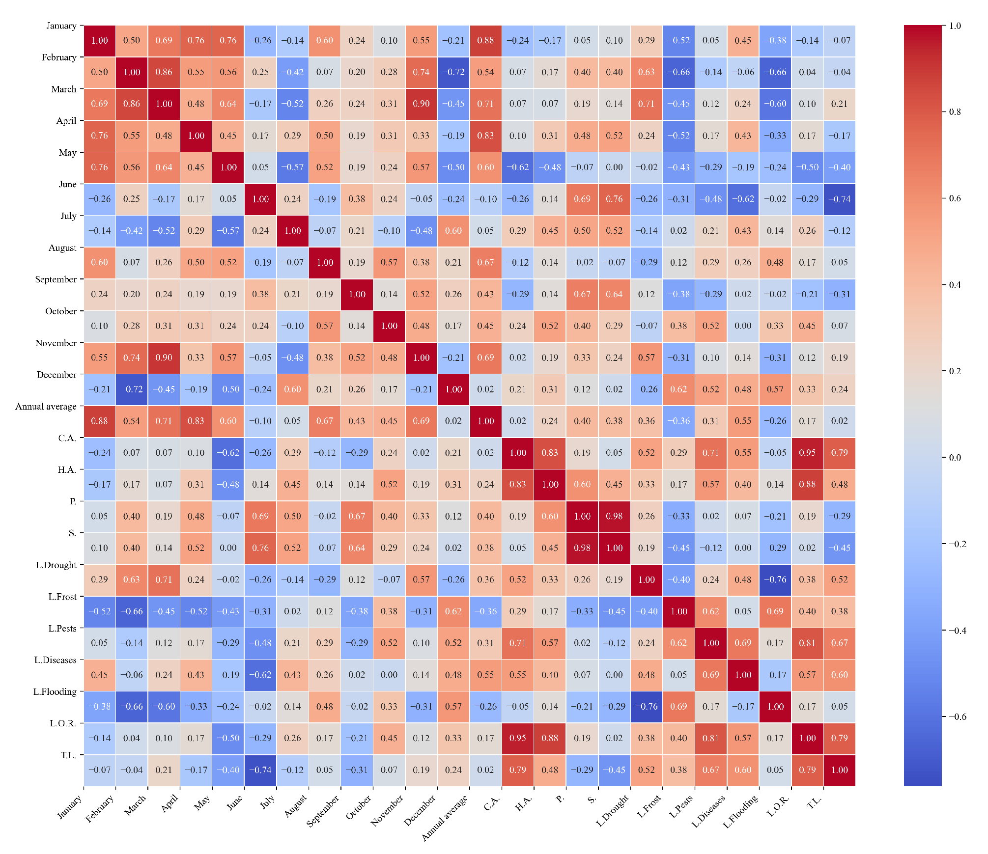
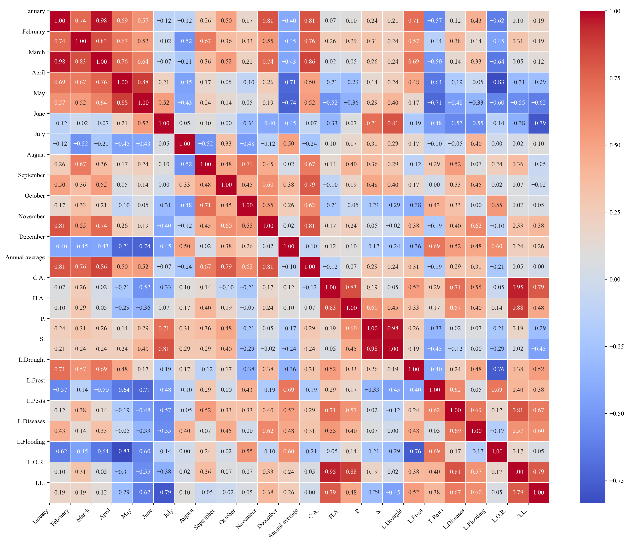
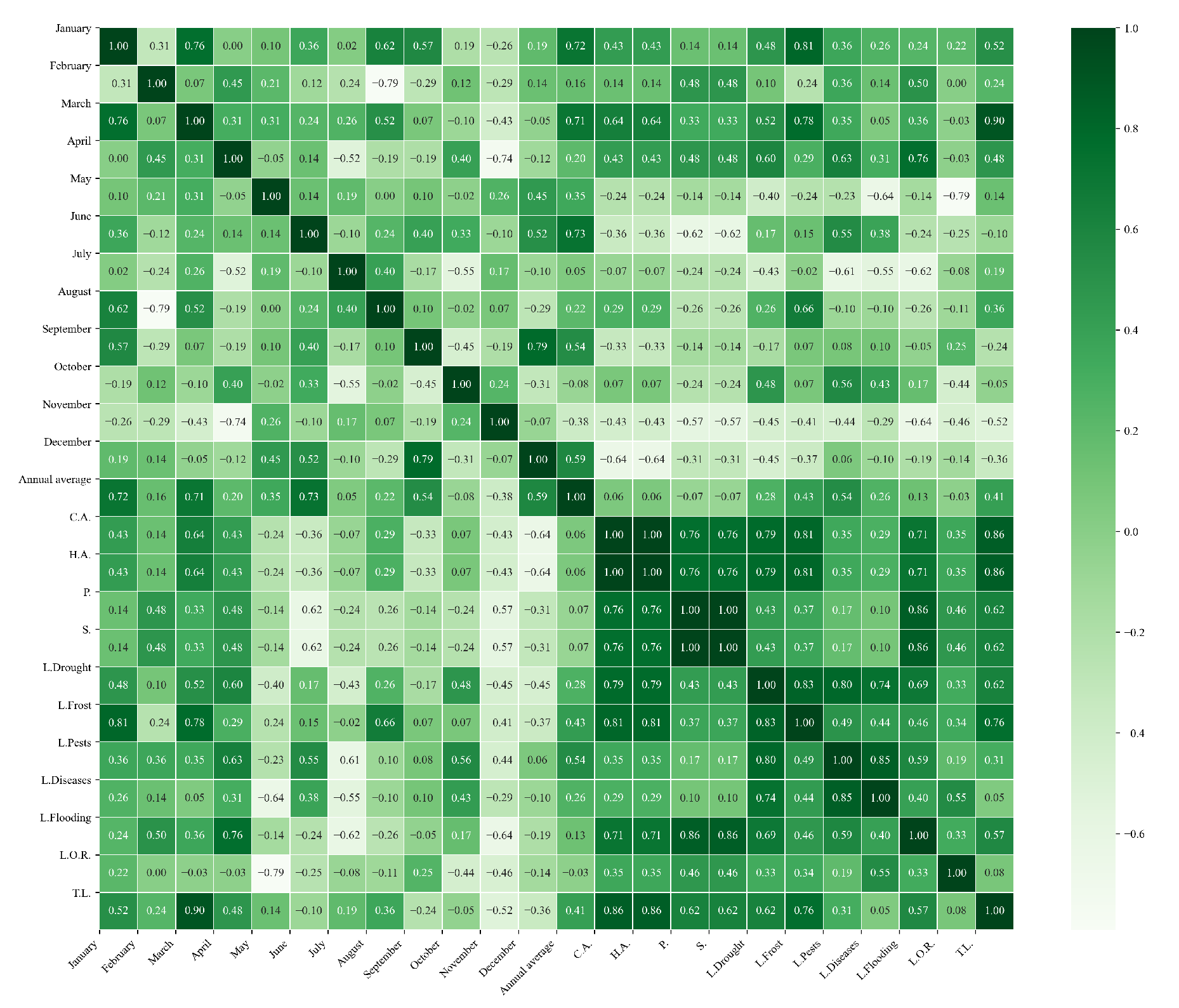
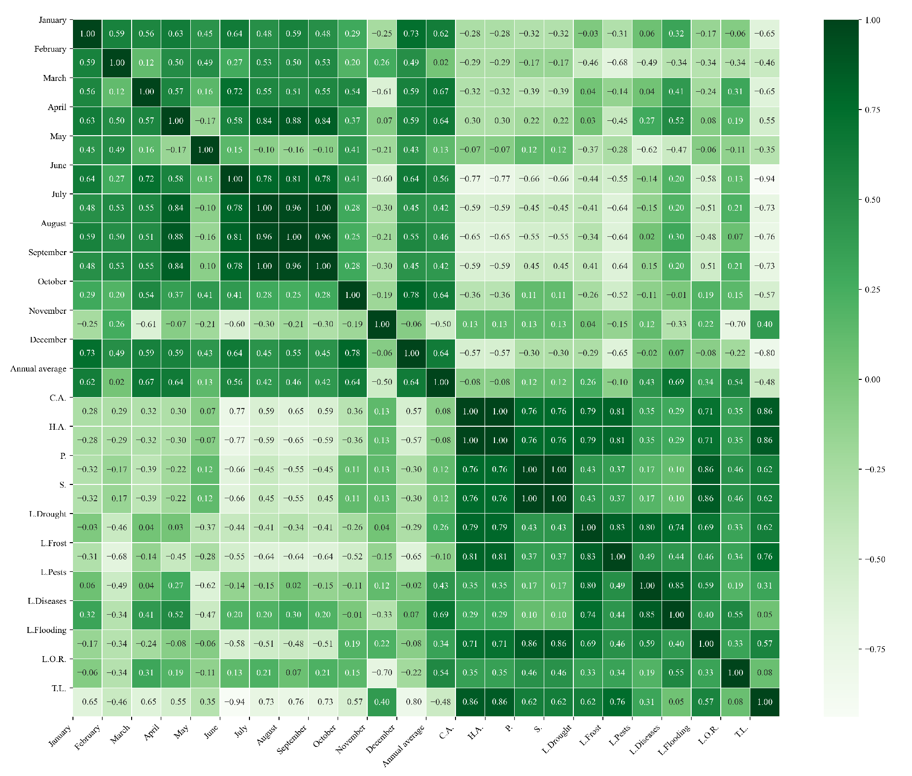
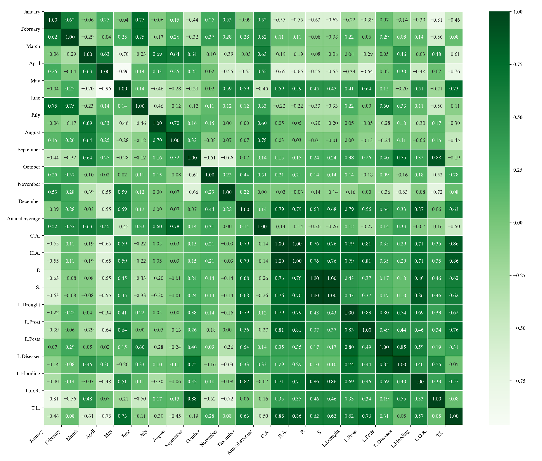
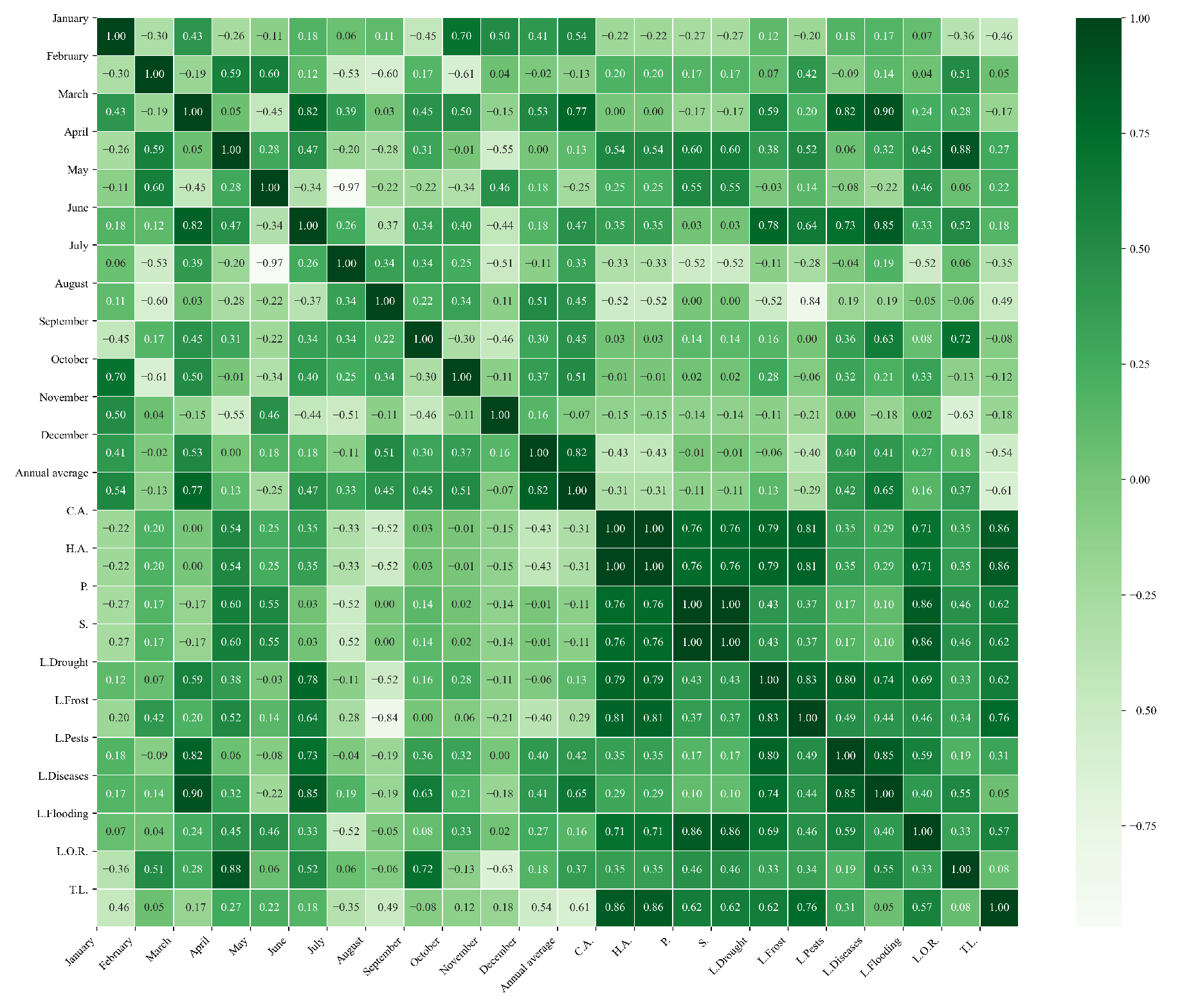
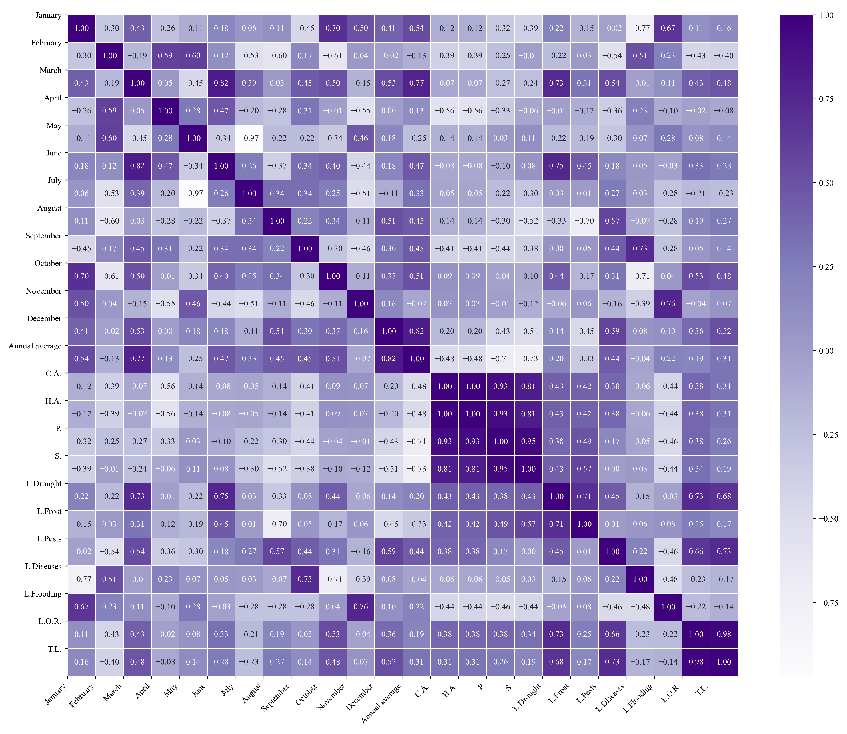
This section presents the correlations between maximum temperature, minimum temperature, and average precipitation in different months of the year and various variables related to quinoa production in the northern, central, and southern zones of Ecuador. Correlation values range from −1 to 1, where 1 indicates a perfect positive correlation, −1 indicates a perfect negative correlation, and 0 indicates no correlation. The analysis focuses on strong positive correlations with a minimum threshold of 0.8 and strong negative correlations with a maximum threshold of −0.8.

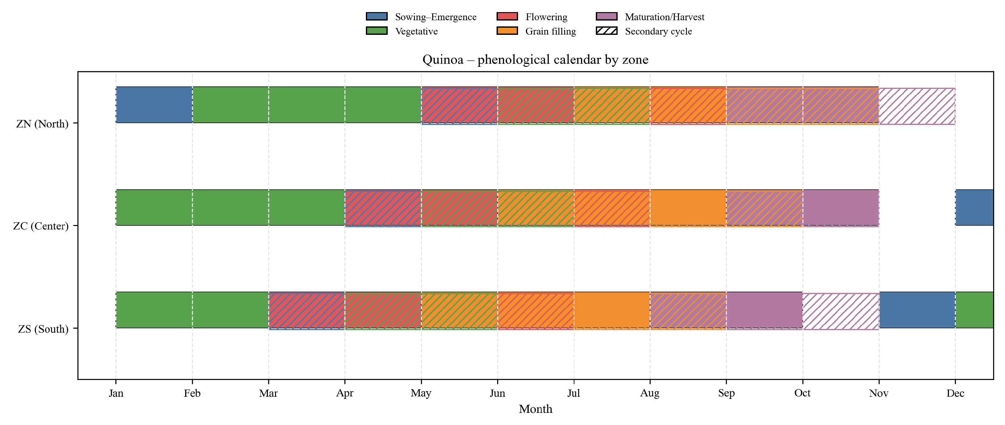
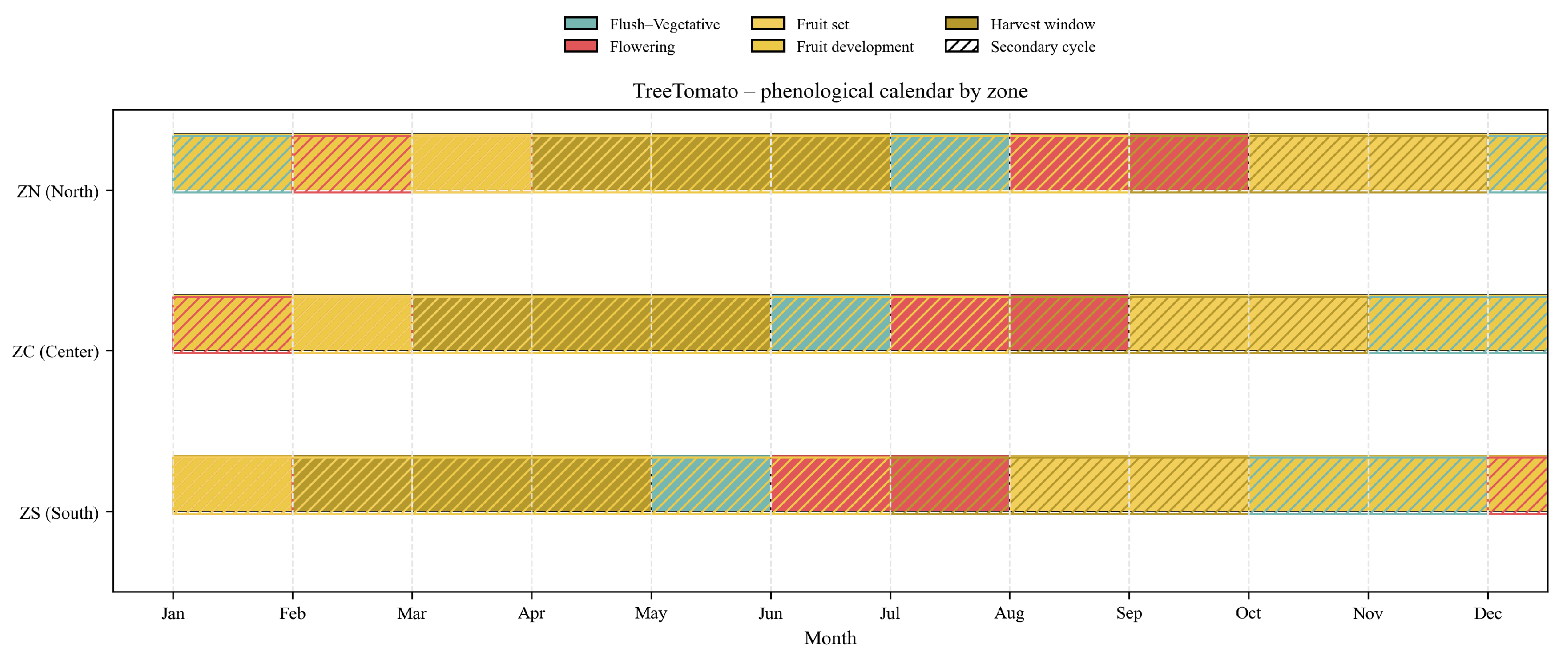
To provide a process-based explanation of significant associations, we align each monthly predictor with quinoa phenology in the Andean highlands. We consider the following phases: sowing–emergence (0–15 DAS), vegetative growth (15–55 DAS), flowering (55–85 DAS), grain filling (85–115 DAS), and maturation/harvest (115–150 DAS). Because cropping calendars vary with altitude and farmer practice, zones typically show (i) a main cycle anchored to the rainy season and (ii) secondary/off-season plantings (including irrigated fields). We therefore interpret each significant month by the phase it most likely overlaps according to the zone-specific calendars (

Table A2. Quinoa phenological calendar by zone (main and secondary cycles). Windows are indicative and may shift with altitude, cultivar, and management.

Zone	Cycle	Sowing–Emergence	Vegetative	Flowering	Grain Filling	Maturation/Harvest
ZN	Main	Jan–Feb	Feb–Apr	May–Jun	Jul–Aug	Sep–Oct
ZN	Secondary	May	Jun–Jul	Aug	Sep–Oct	Nov
ZC	Main	Dec–Dec; Jan–Jan	Jan–Mar	Apr–May	Jun–Aug	Sep–Oct
ZC	Secondary	Apr	May–Jun	Jul	Aug–Sep	Oct
ZS	Main	Nov–Dec	Dec–Dec; Jan–Feb	Mar–Apr	May–Jul	Aug–Sep
ZS	Secondary	Mar	Apr–May	Jun	Jul–Aug	Sep–Oct

, Figure A2). This mapping is used only to contextualize correlations and does not alter the statistical results.

4.2.1. Maximum Temperature in the Northern, Central, and Southern Zones

• Northern zone

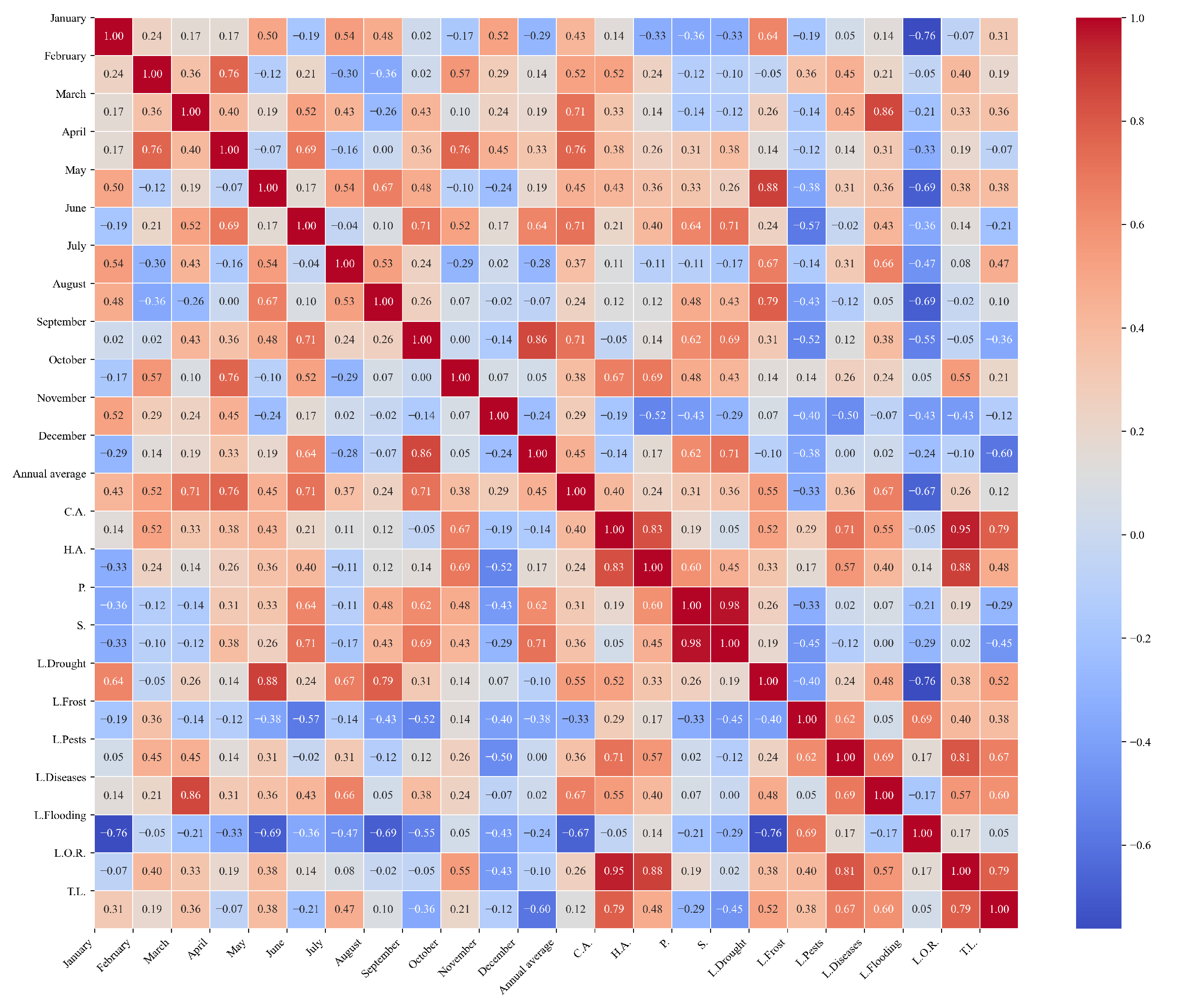
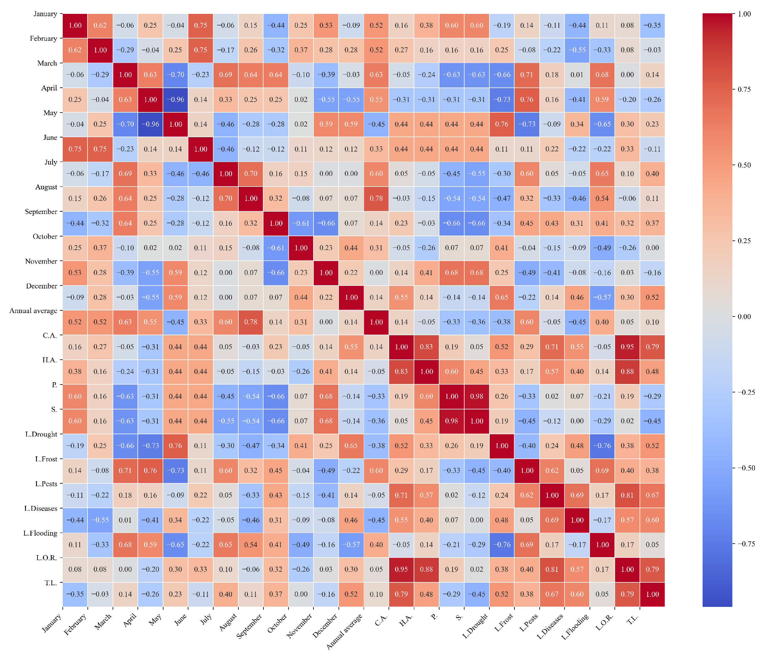
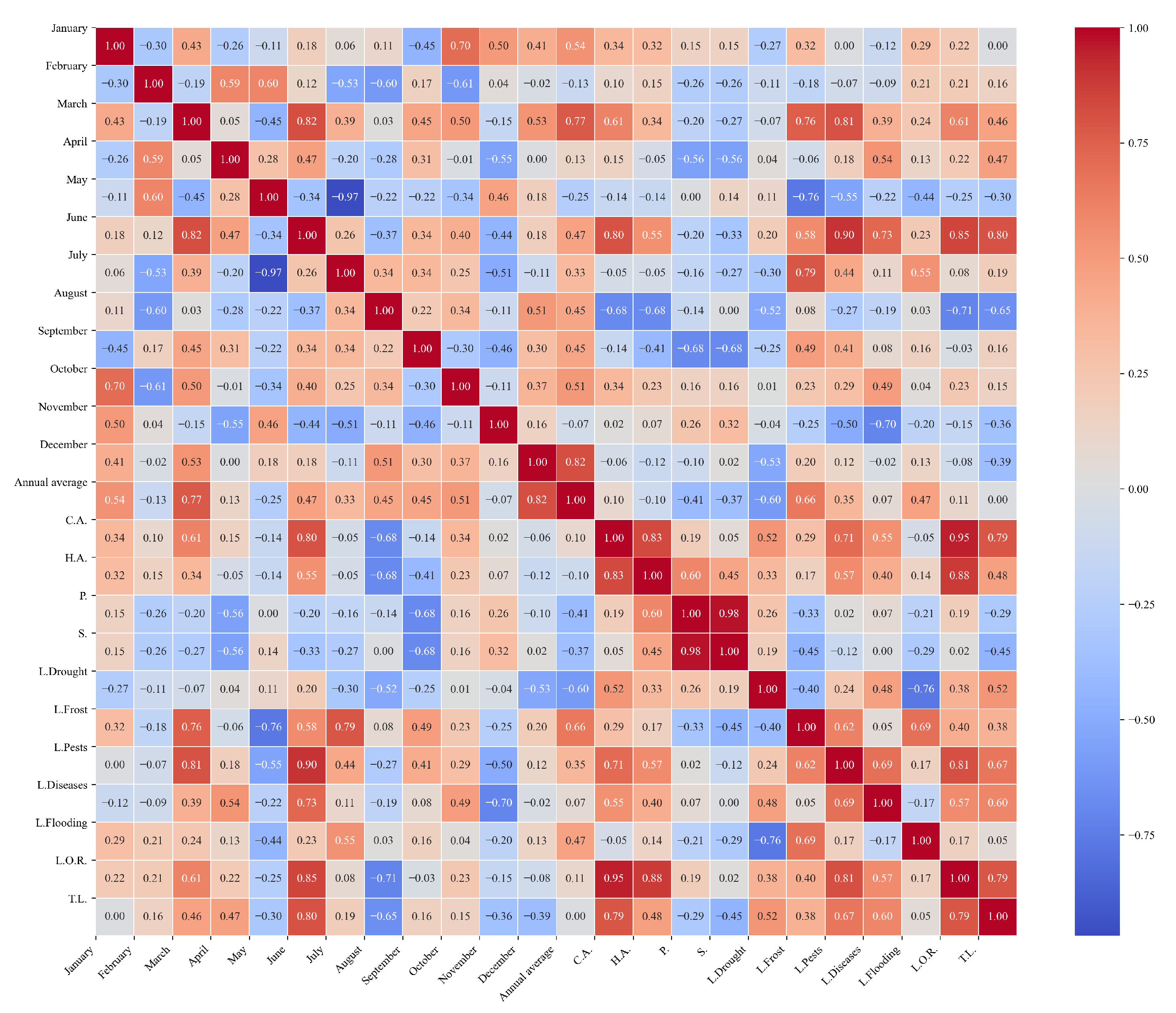
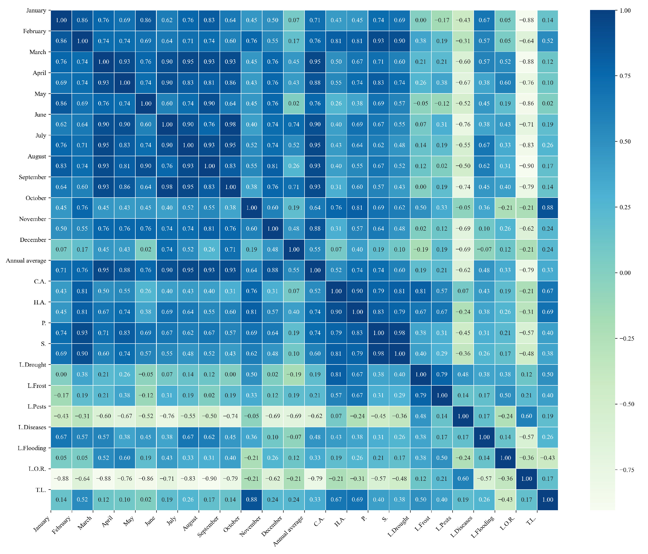
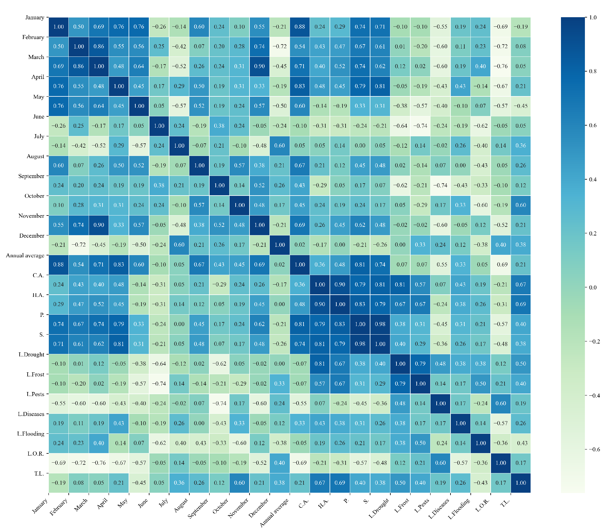
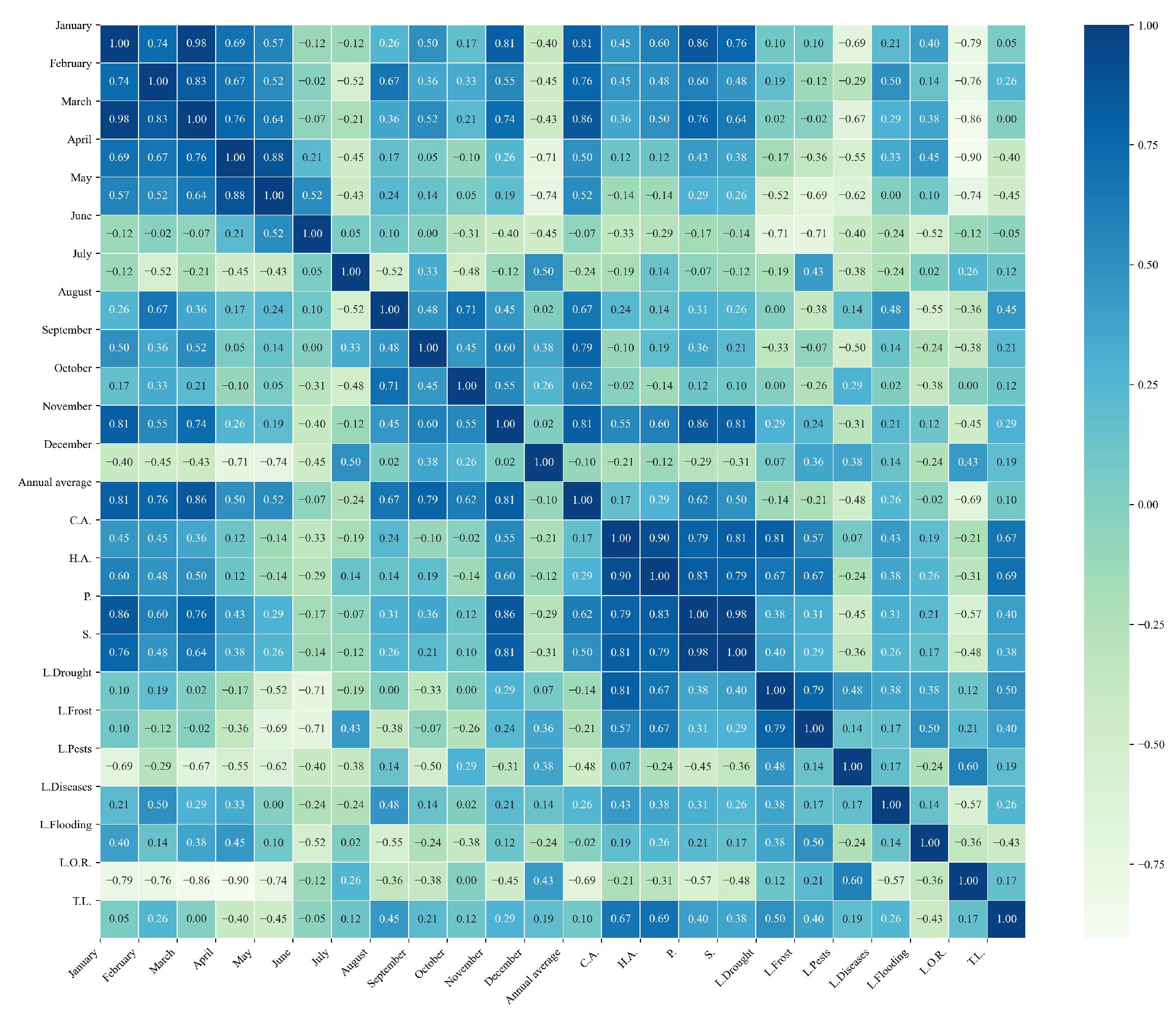
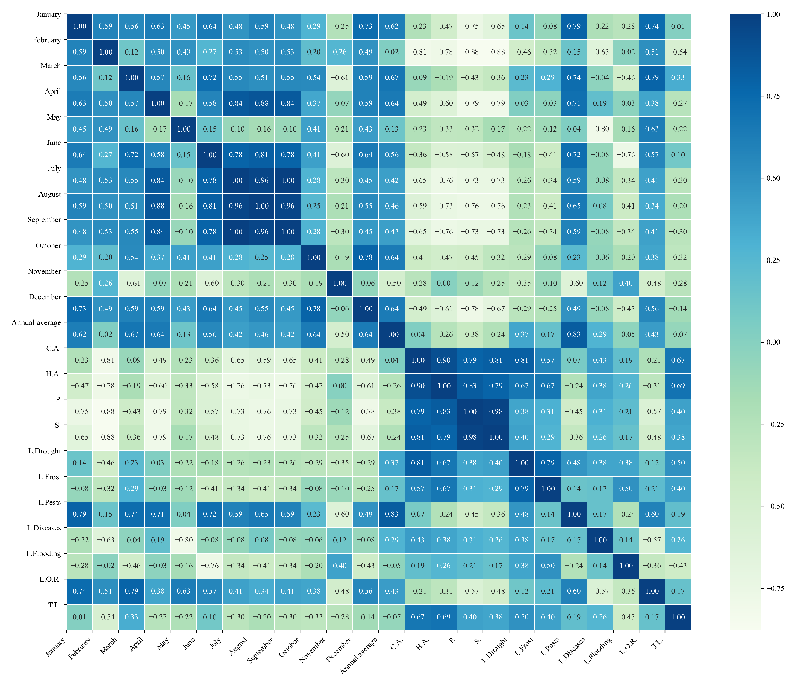
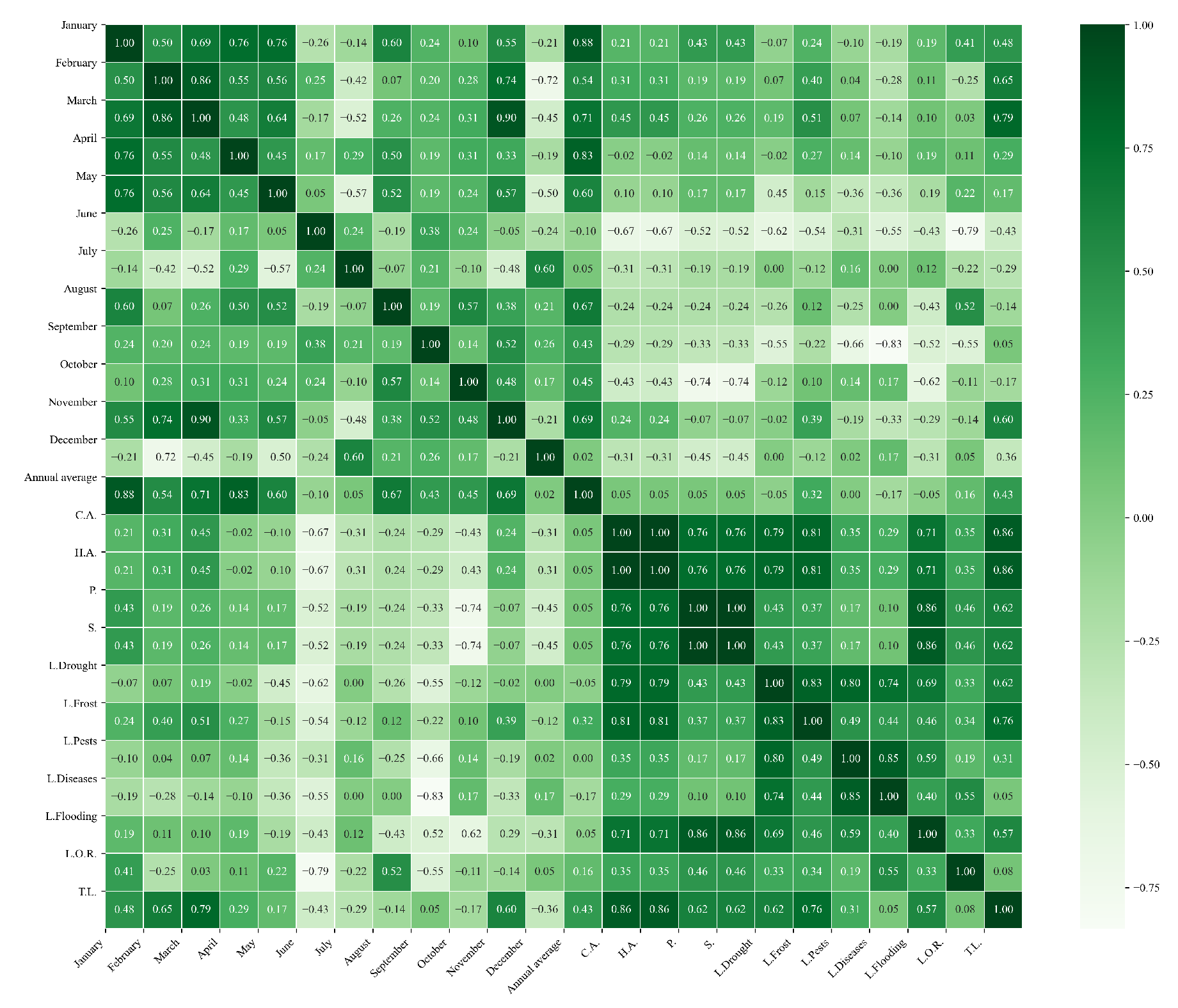
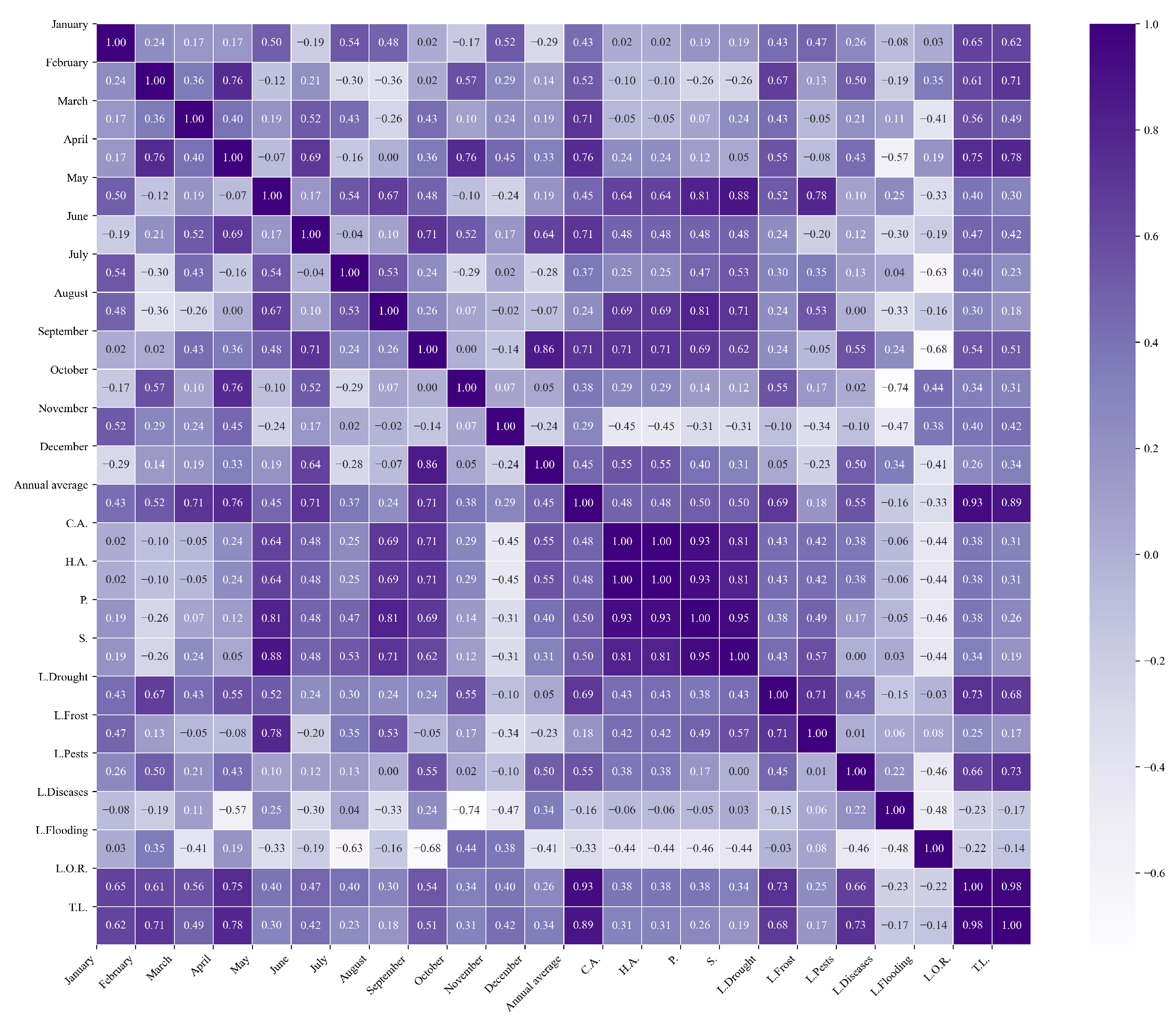
Figure 10, shows the correlations of the variables in the northern zone. Significant correlations were identified between maximum temperatures and the agricultural variables C.A., H.A., P., and S. in the months of July, September, and November. These strong correlations suggest that maximum temperatures during these months have a direct impact on quinoa yield. For instance, higher temperatures in July may be associated with larger cultivated and harvested areas, directly influencing production and sales. Similarly, the correlations observed in September and November highlight the importance of these months in the quinoa growth and harvest cycle, where higher temperatures may play a crucial role in maximizing agricultural yield.

In ZN, the months highlighted by the analysis (July, September, November) most often overlap with late vegetative to early flowering (July), peak flowering/early grain filling (Sep), and late filling to pre-harvest (Nov) in the dominant calendars (Table A2). Within agronomic ranges, warmer daytime conditions in these windows enhance thermal time accumulation, reduce frost exposure at critical reproductive stages, and help reach physiological maturity, which is consistent with the positive correlations with C.A., H.A., P., and S.

In addition, significant correlations are observed between maximum temperatures in different months. The correlation of $0.908$ between January and May suggests continuity in high temperatures during these months, indicating that climatic conditions in January are likely to influence temperatures observed in May. This pattern is relevant for agricultural planning, as it enables forecasting of the potential impact that high temperatures at the beginning of the year may have on the subsequent season. Likewise, the correlation of $0.880$ between January and August reinforces the idea that high temperatures in January have a prolonged effect on the annual climate cycle. Furthermore, the correlation of $0.953$ between March and June highlights the importance of monitoring conditions during the sowing and growth season, as it suggests that maximum temperatures in March may directly influence those in June, a crucial month for quinoa development. Additionally, the correlation of $0.957$ between May and August underscores the relationship between temperatures in these key months, which can affect the final cultivation phase and preparation for harvest.

The strong associations between L.Frost and several months align with the mechanistic role of temperature at reproductive stages: higher Tmax during late winter–spring reduces the probability of damaging night frosts around flowering and early filling, thereby lowering losses and supporting higher production and sales.

• Central zone

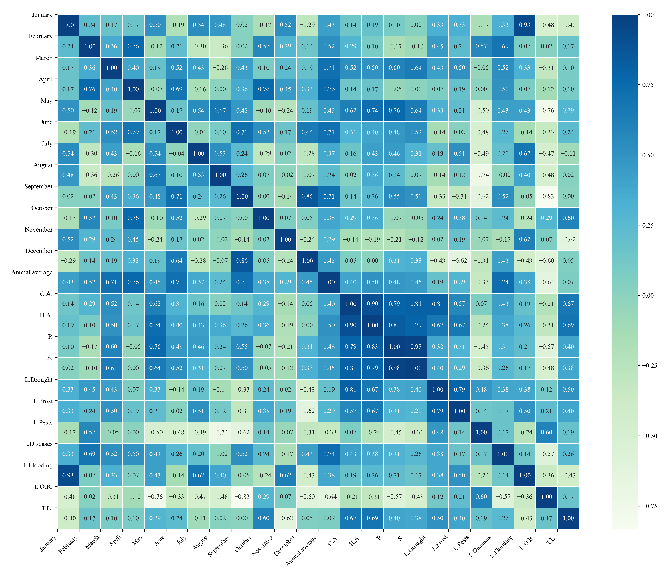
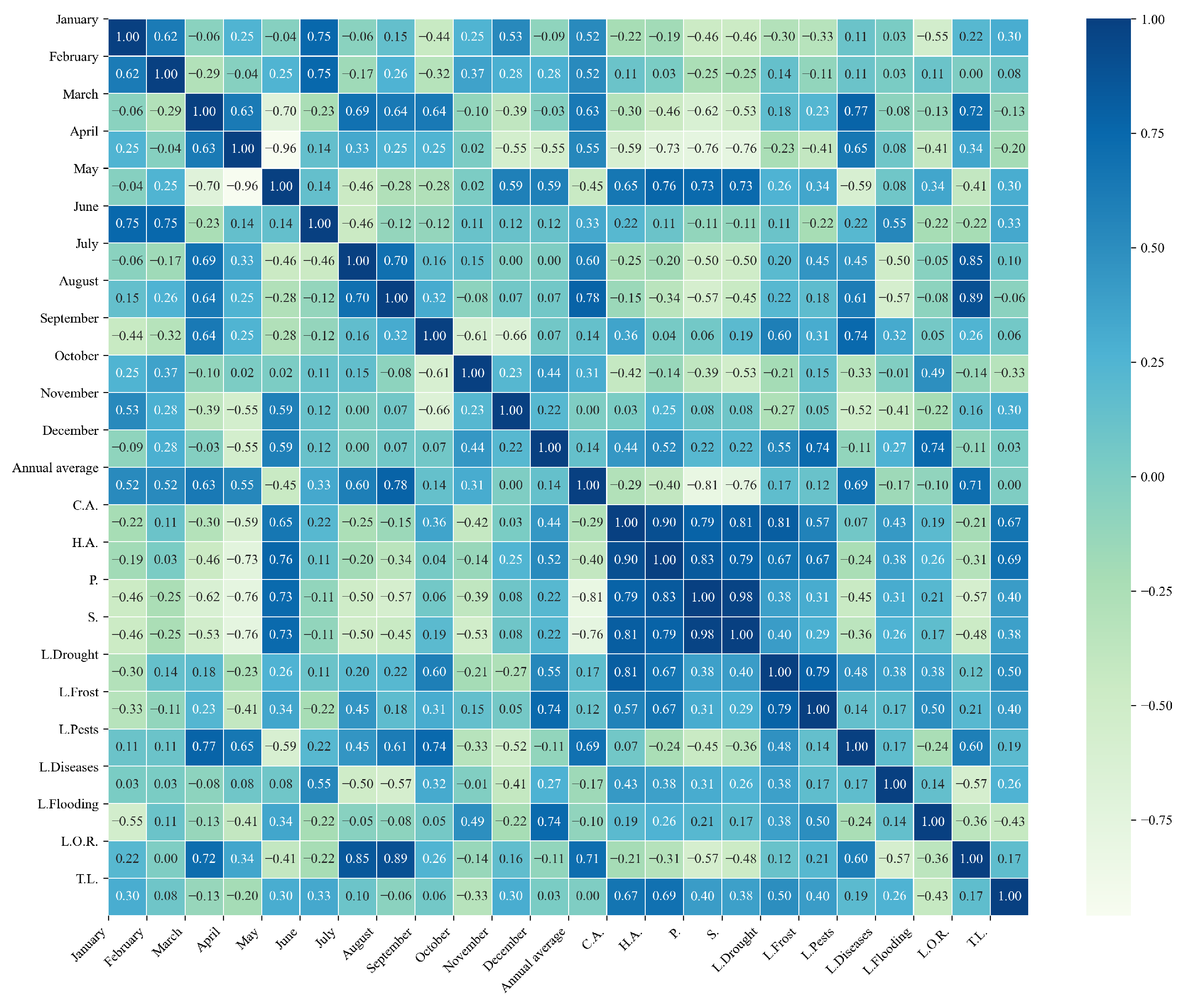
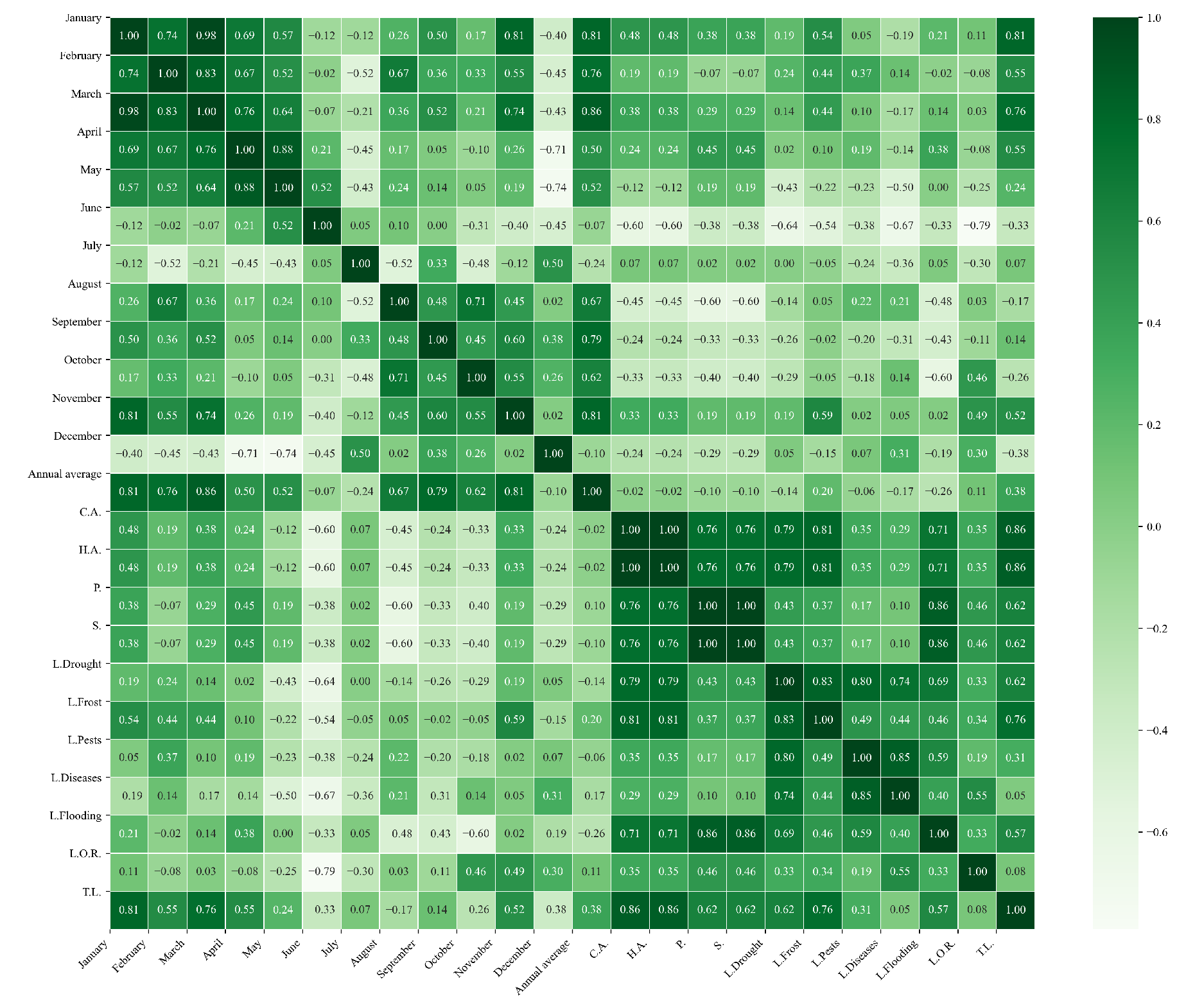
In the central zone, maximum temperatures also show notable correlations, as illustrated in Figure 11. Temperatures in certain months are highly correlated, suggesting that climatic conditions in one month can have a prolonged effect on subsequent months. For example, a correlation of $0.8616$ between February and March indicates continuity in climatic conditions between these two months, which are crucial for the early development of quinoa. Similarly, the correlation of $0.8079$ between January and April suggests that temperatures at the beginning of the year may influence spring climatic conditions, affecting soil preparation and sowing.

These correlations between temperatures are important because they reflect the climatic stability or variability that farmers must consider when planning the crop cycle. The ability to anticipate how conditions in one month will influence the following months enables farmers to adjust crop management strategies to optimize yields during the season.

In ZC, February–March typically straddle late vegetative to floral initiation, while August often coincides with grain filling or late reproductive development for the main cycle and with vegetative stages in off-season plantings. The observed links between Tmax (Feb–Mar, Aug) and production/sales are therefore consistent with thermal requirements during reproductive development and the completion of grain filling.

Regarding the agricultural variables, significant correlations are observed, particularly between L.Frost and the variables C.A., H.A., P., and S. These correlations indicate that frost losses have a strong relationship with cultivated area, harvested area, production, and sales.

For example, a high correlation between L.Frost and C.A. suggests that as the area dedicated to cultivation increases, exposure to frost losses also rises. This could be due to greater vulnerability in extensive areas or the difficulty of effectively implementing preventive measures on a large scale.

Similarly, the strong correlation between L.Frost and P. indicates that frost events directly impact crop yield. These losses affect not only production but also S., underscoring the importance of managing climatic risks to safeguard the profitability of quinoa cultivation.

Temperatures also show some correlations with agricultural variables. Although no extremely high correlations were found, identifying relationships such as the correlation between temperatures in certain months and variables like P. or L.Drought can be useful for adjusting management strategies during the season.

These correlations underscore the importance of efficient climate management during key months of the agricultural cycle. Decisions made in critical periods can influence the final yield and the profitability of the crop.

• Southern zone

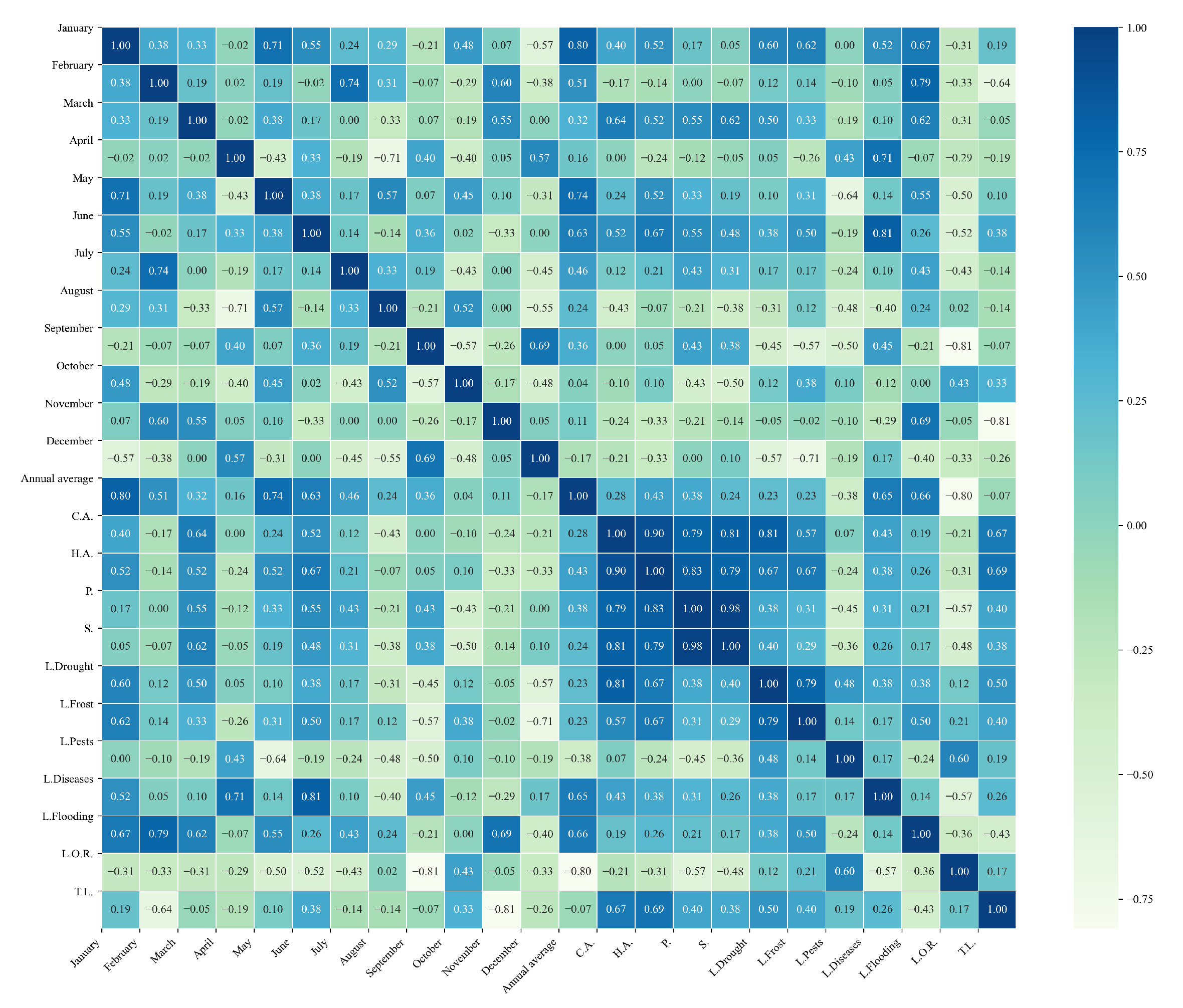
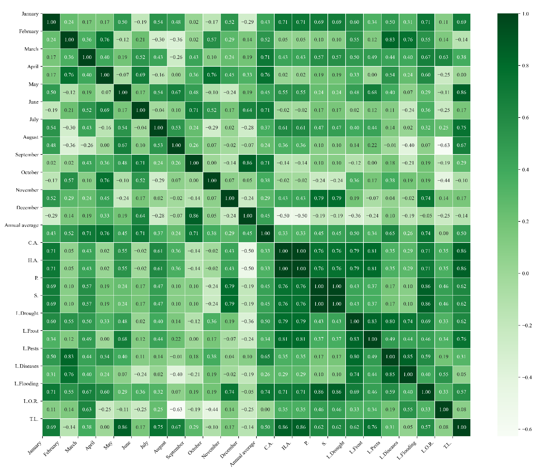
In the southern zone, Figure 12 shows that maximum temperatures exhibit significant correlations with several agronomic variables. Temperatures in certain months are highly correlated, suggesting that climatic conditions in one month can have a direct impact on the following months. A notable example is the correlation of $0.9201$ between January and March, indicating that temperatures at the beginning of the year have a prolonged influence until the third month, which can be critical for the crop establishment stage. January–April in ZS commonly span establishment (Jan) through vegetative growth and flowering (Mar–Apr). Positive associations of Tmax in these months with production variables are consistent with faster canopy development and timely transition to reproduction, provided temperatures remain within crop optima. Additionally, the correlation of $0.8050$ between March and April reinforces this idea, showing continuity in climatic conditions during the transition to spring.

Another significant correlation is found between April and May ($0.8397$), suggesting that early spring climatic conditions have a lasting impact on the climate of subsequent months, which is critical for soil preparation and the initial growth phases of quinoa.

In this dataset, strong correlations were identified between L.Frost and the variables C.A., H.A., P., and S. This indicates that frost losses have a direct impact on cultivated area, harvested area, production, and sales. As frost events intensify, a decrease in these agricultural variables is observed, underscoring the vulnerability of quinoa cultivation to extreme climatic conditions.

In addition, a significant correlation is identified between L.O.R. and T.L. This relationship suggests that external factors, such as logistical or management issues, have a considerable impact on total losses, highlighting the need for mitigation strategies that address not only climatic risks but also other operational factors.

Although no extremely high correlations have been identified between temperatures and agricultural variables, the influence of climatic conditions on frost losses underscores the importance of effective climate management. The continuity of climatic conditions throughout the months can indirectly influence agricultural yield, particularly with respect to temperatures during critical months of the quinoa crop cycle.

4.2.2. Minimum Temperature in the Northern, Central, and Southern Zones

• Northern zone

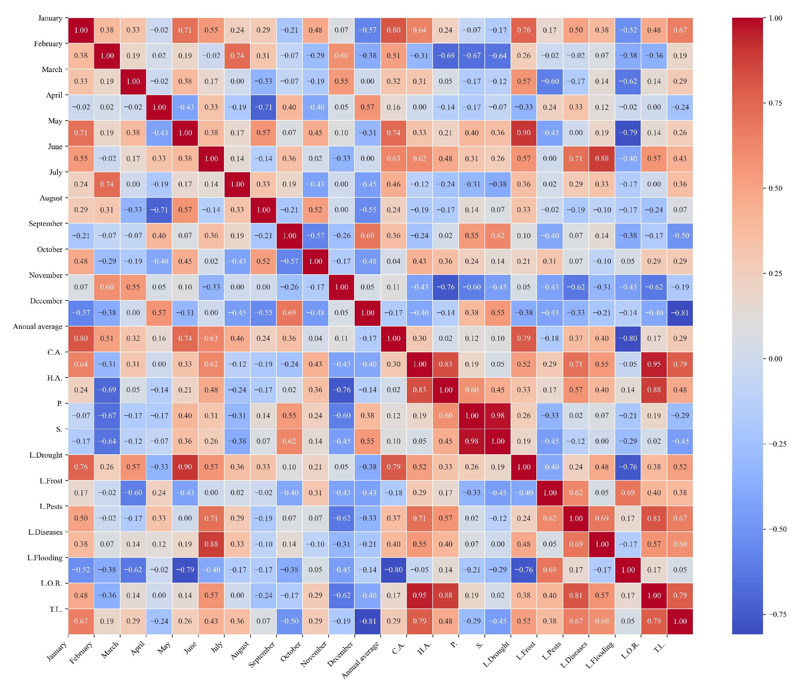
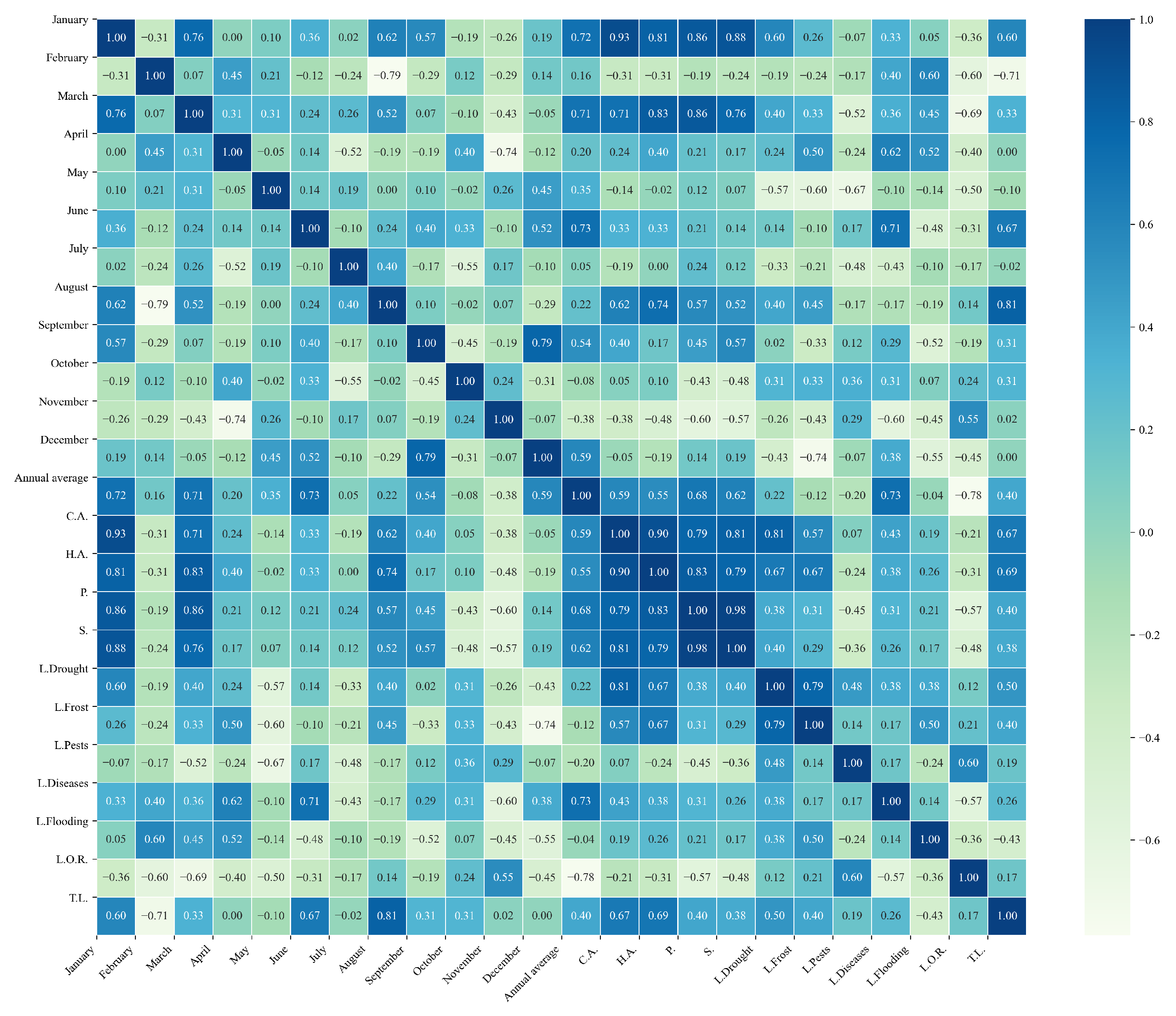
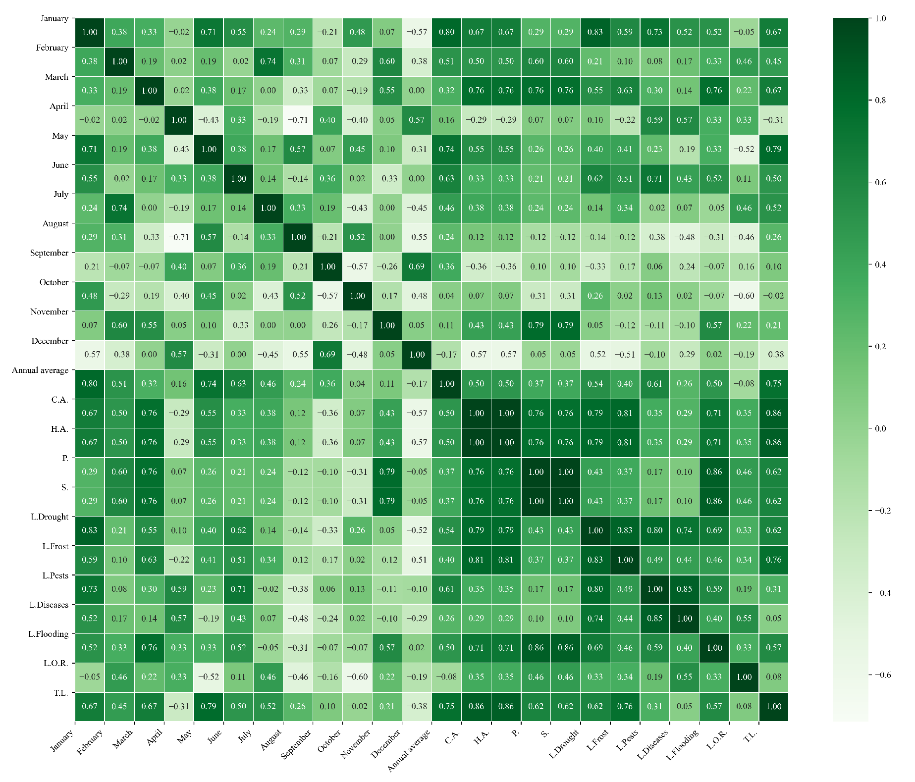
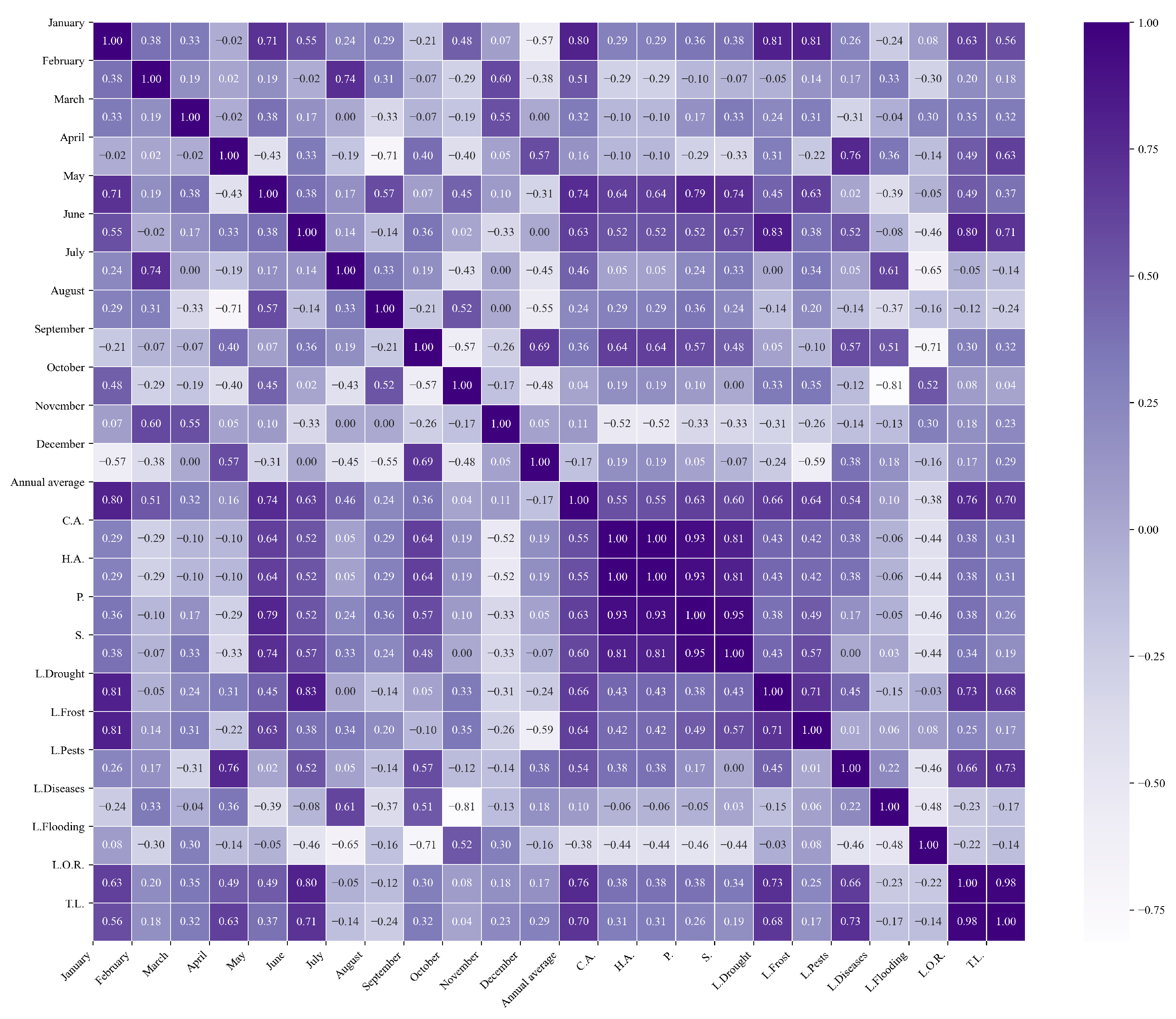
In the northern zone, minimum temperatures show moderate to strong correlations with certain variables, as illustrated in Figure 13. Average minimum temperatures in different months present some significant correlations. For example, a correlation of $0.8622$ is observed between April temperatures and the annual mean. This value indicates that April conditions are strongly aligned with the annual climatic behavior in the analyzed zones. Similarly, December and September temperatures have a correlation of $0.8535$, suggesting that end-of-year climate influences September conditions, which may have implications for crop preparation for the next cycle.

These correlations are important because they reflect climatic stability or variability at different times of the year, which is crucial for farmers when planning cultivation activities. The ability to predict how climatic conditions in one month may affect subsequent months allows for more effective adjustment of crop management strategies.

Regarding the agricultural variables, a strong correlation of $0.9944$ is observed between C.A. and H.A., suggesting high efficiency in land management. This value indicates that most of the area allocated to quinoa cultivation is harvested, reinforcing the importance of effective planning from the beginning of the agricultural cycle.

Another notable correlation is between P. and S., with a value of 0.9880. This shows that production is closely linked to sales, consistent with the expectation that production determines the supply available to the market. In addition, the correlation of 0.9191 between L.Frost and production suggests that frost has a significant impact on the final quantity of quinoa produced. This underscores the need for strategies to mitigate the negative effects of frost.

Temperatures also show significant correlations with agricultural variables. For example, the correlation of 0.9118 between August temperatures and P. indicates that climatic conditions in August influence quinoa yield. This month, which is crucial for quinoa development, can determine the final quantity produced. Similarly, August temperatures are correlated with L.Frost ($0.8177$), highlighting the importance of climatic conditions during this period.

• Central zone

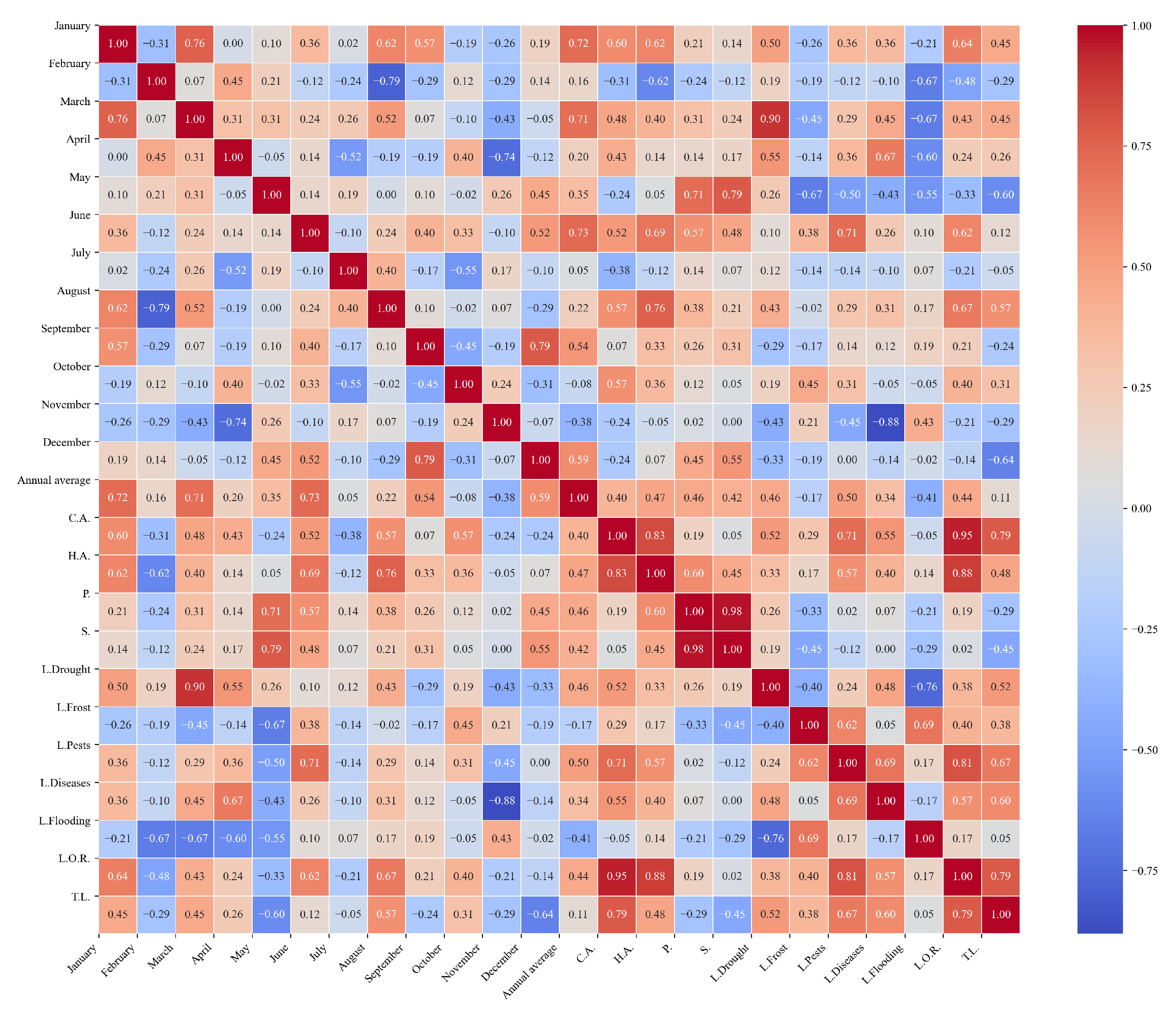
In the central zone, as shown in Figure 14, minimum temperatures also show significant relationships. The correlation of $0.8484$ between L.Frost and C.A. suggests that as the area dedicated to cultivation expands, frost losses also increase. This indicates that larger-scale production is directly associated with greater vulnerability to frost, which may pose additional risks for large-scale production. Similarly, the correlation of $0.8177$ between L.Frost and H.A. reflects that larger harvested areas are also exposed to greater frost losses, underscoring the importance of planning climate mitigation strategies as production expands.

In ZC, March and August align with floral development and early filling in the main cycle. Higher Tmin in March is associated with increased disease pressure (favorable humidity and night-time leaf wetness), whereas warmer Tmin in August supports grain filling; both patterns are coherent with the signs and magnitudes observed for losses and production/sales.

P. shows a correlation of $0.9191$ with losses due to frost, indicating that this climatic phenomenon has a significant impact on agricultural yield. As production increases, so does the risk that frost will negatively affect outcomes, reinforcing the need for effective climate management. Likewise, the correlation of $0.9292$ between L.Frost and S. demonstrates that frost not only impacts production but also has a direct effect on product marketing, affecting revenue from sales.

On the other hand, the negative correlation of $-0.8651$ between L.Diseases and October temperatures suggests that crop diseases tend to decrease during this month. This pattern may be related to seasonal factors that reduce the incidence of diseases, potentially due to changes in climatic conditions or in agricultural practices implemented during this period.

Regarding the relationship between temperatures and agricultural variables, the correlation of $0.8033$ between P. and August temperatures stands out. This finding suggests that climatic conditions in August are favorable for quinoa crop development, directly impacting the quantity of harvested product. Similarly, the correlation of $0.8004$ between S. and August temperatures reinforces the idea that climatic conditions in this month are critical not only for production but also for crop marketing.

The correlation of $0.8004$ between L.Drought and June temperatures indicates that this month is crucial for climate risk management. Droughts in June can have a considerable impact on agricultural losses, underscoring the need for preventive planning during this key month. In addition, the correlation of $0.8188$ between L.Diseases and March temperatures suggests that this period is critical for the onset of diseases affecting quinoa cultivation. Minimum temperatures in March appear to be associated with an increase in losses due to diseases, highlighting the importance of sanitary management during this month to minimize adverse effects on production.

• Southern zone

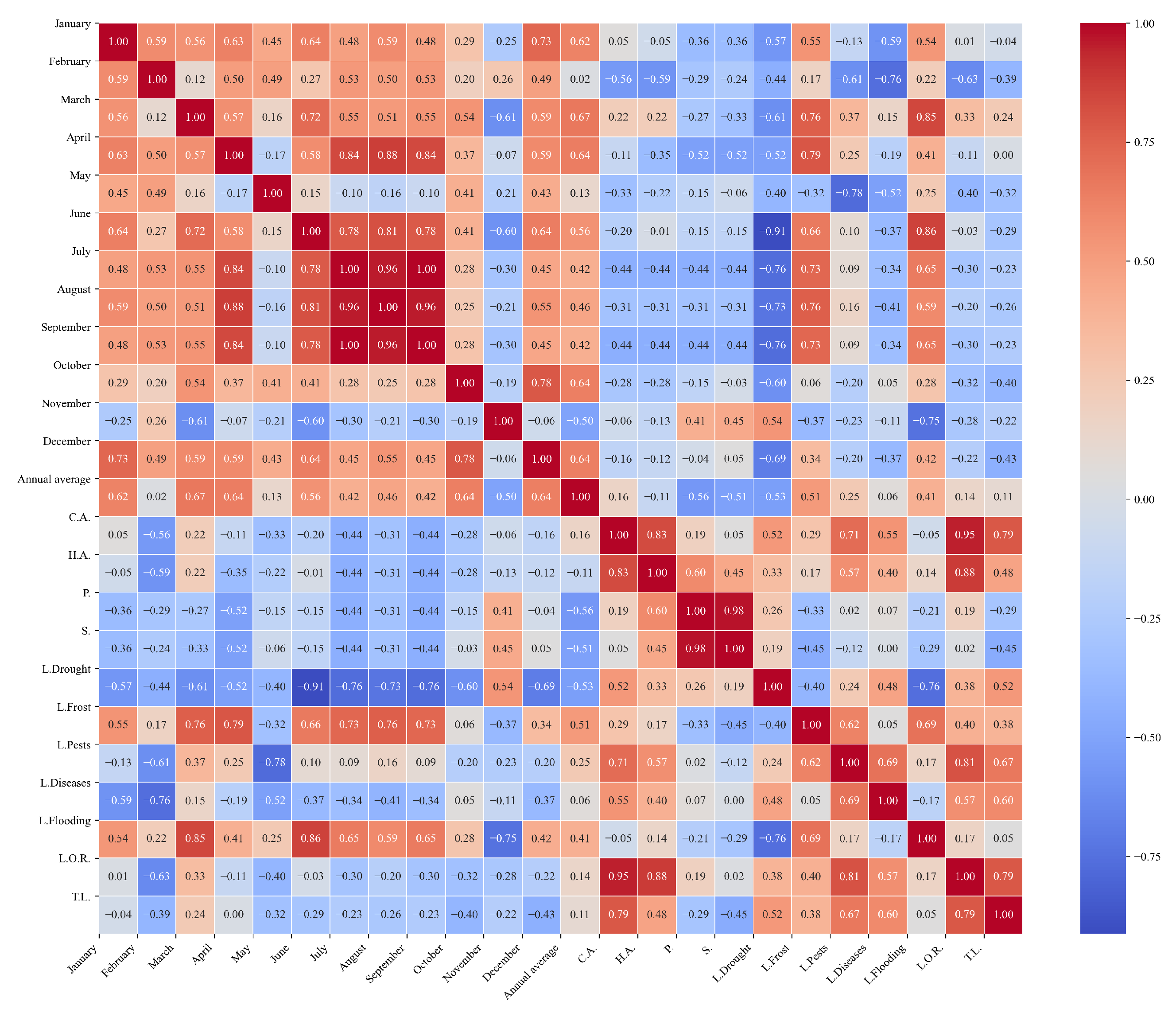
In the southern zone, Figure 15 shows that minimum temperatures present some noteworthy correlations. The correlation of $0.9542$ between L.O.R. and T.L. indicates that a large share of total losses in quinoa cultivation is attributable to non-specific factors, such as logistical, operational, or management issues. This finding highlights the need to focus efforts not only on mitigating direct losses from climate, pests, or diseases but also on improving processes and infrastructure that indirectly affect agricultural yield.

In ZS, January corresponds to establishment–early vegetative growth; higher Tmin in this period favors pathogen development and survival, which is consistent with the positive association between January Tmin and L.Diseases. Conversely, warmer September nights during the late season reduce flooding-related losses, as the rainy peak weakens and evaporative demand increases.

Regarding Losses due to Frost (L.Frost), a high correlation is observed with the main production variables: C.A. ($0.8484$), H.A. ($0.8177$), P. ($0.9191$), and S. ($0.9292$). These relationships suggest that frost has a considerable impact on all stages of quinoa production and marketing. As the scale of production increases, so does exposure to frost risk, underscoring the importance of implementing preventive measures and climate risk mitigation strategies to protect large-scale production.

The analysis also highlights the correlation of $0.8186$ between January and L.Diseases, suggesting that climatic conditions in January are strongly related to the incidence of diseases in quinoa crops. This positive correlation indicates that an increase in temperature severity in January could be associated with a higher risk of diseases, emphasizing the need for proactive sanitary management during this critical month of the agricultural cycle.

On the other hand, the negative correlation of $-0.8480$ between September and L.Flooding suggests that warmer temperatures in September are associated with reduced flooding losses. This finding indicates that during this month, climatic conditions tend to be more favorable, potentially lowering the risk of water damage and providing a more stable environment for crop growth.

4.2.3. Average Precipitation in the Northern, Central, and Southern Zones

• Northern zone

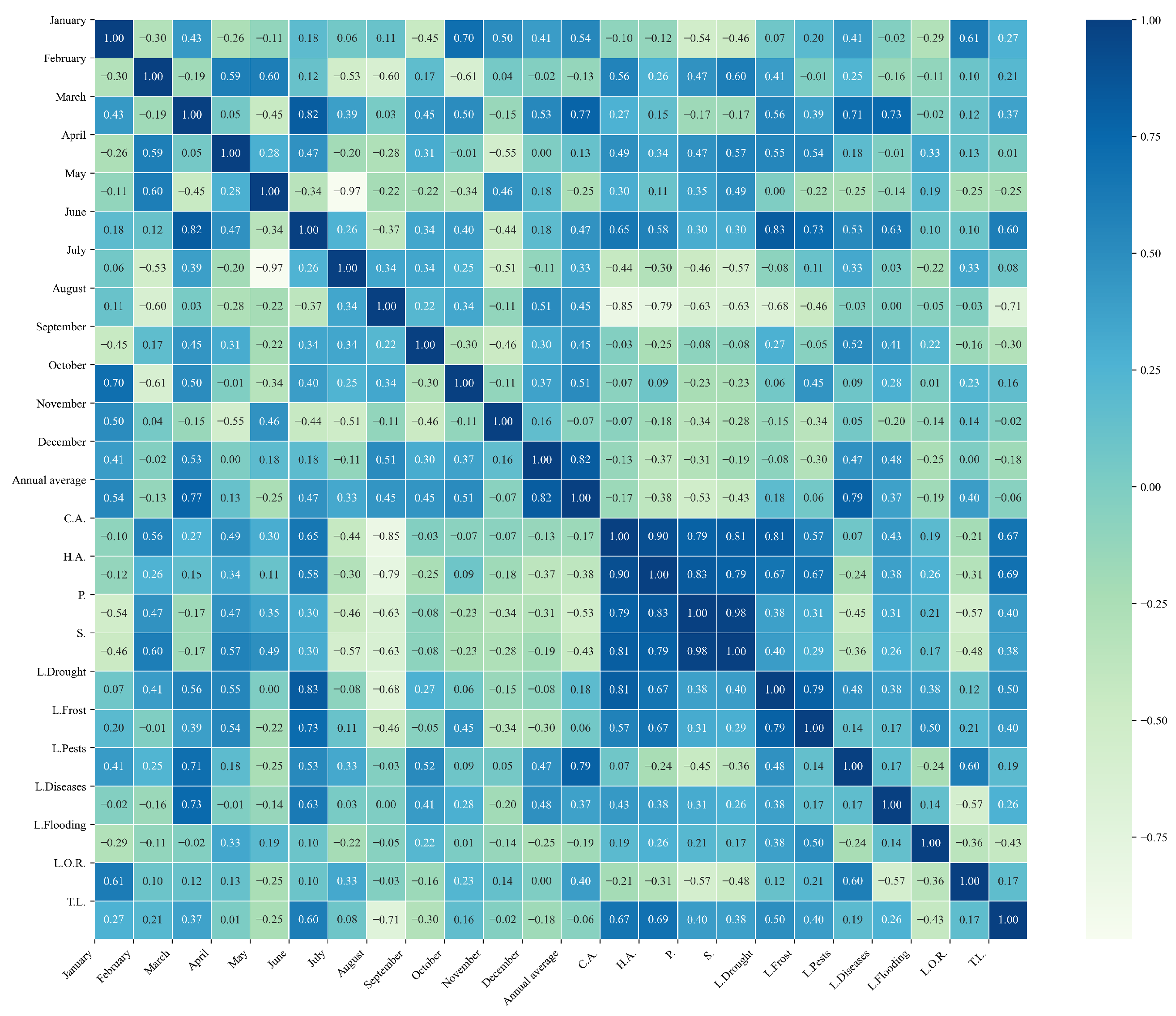
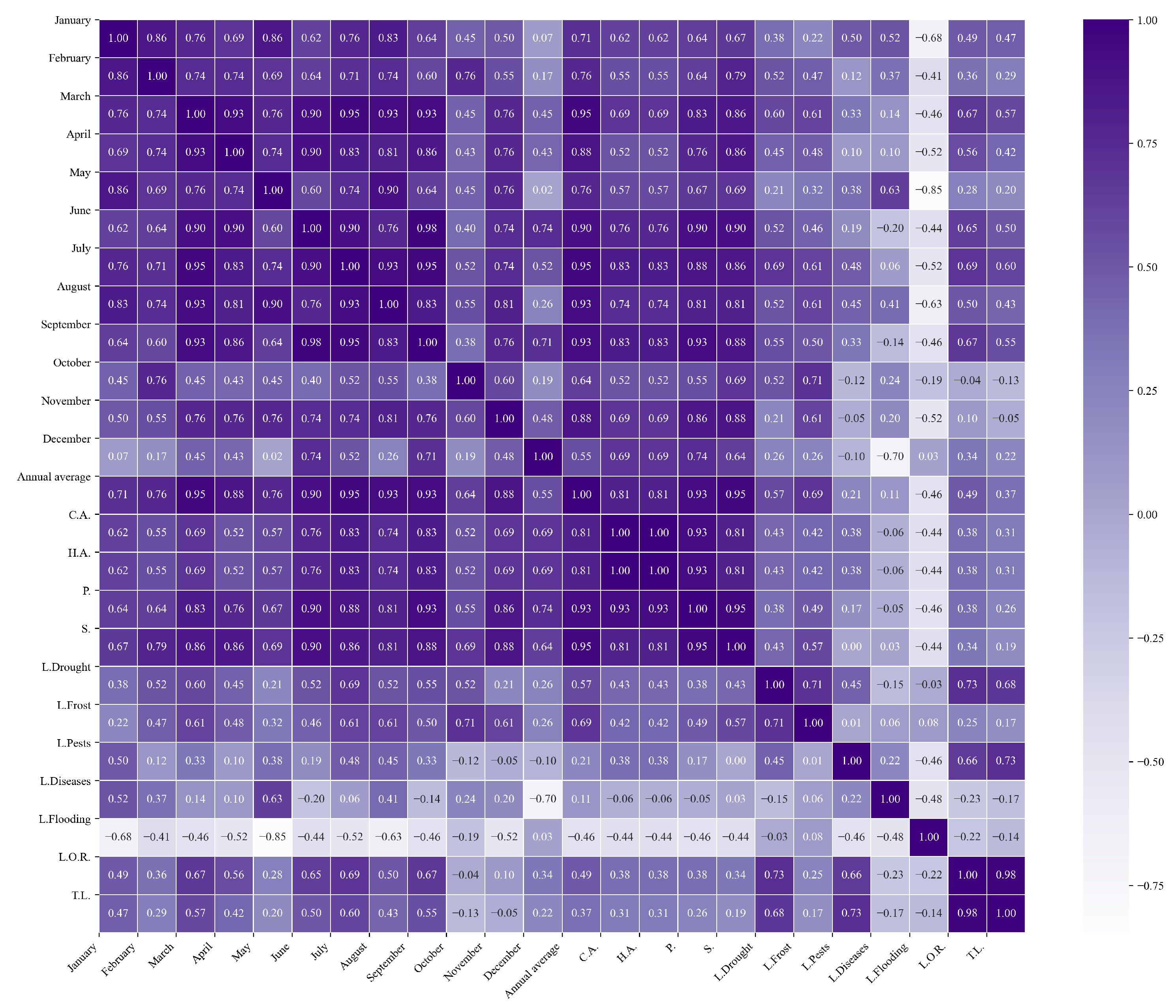
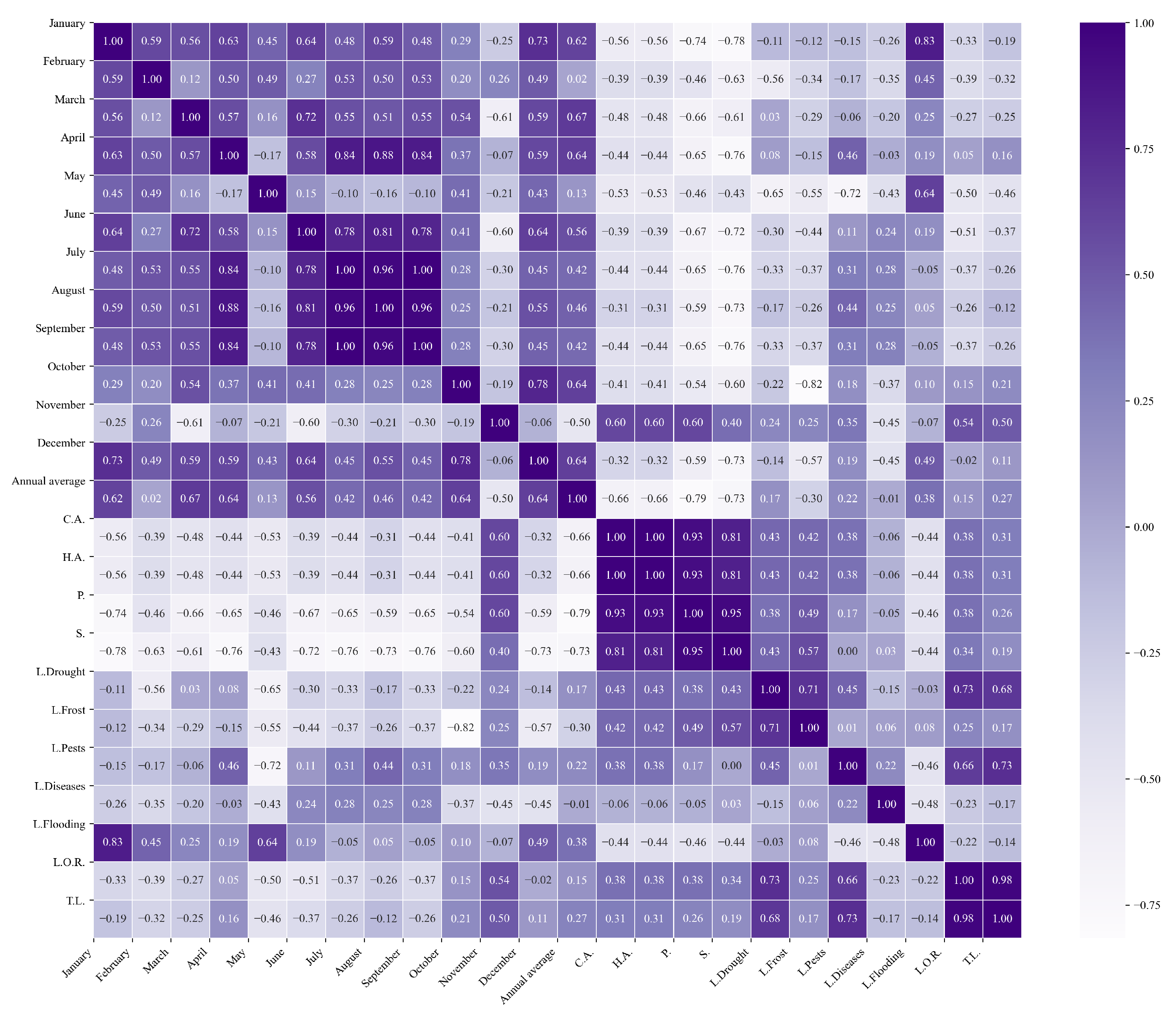
In the northern zone, average precipitation shows varied correlations with production variables, as illustrated in Figure 16. A strong correlation of $0.9542$ is observed between L.O.R. and T.L. This suggests that a significant portion of total losses in quinoa cultivation is attributable not to climatic or biological factors but to other causes, such as logistical, operational, or management issues. This finding highlights the importance of improving internal processes and infrastructure to reduce losses that are not directly related to environmental conditions.

On the other hand, L.Frost show important correlations with several agricultural variables: C.A. ($0.8484$), H.A. ($0.8177$), P. ($0.9191$), and S. ($0.9292$). These correlations indicate that frost significantly affects all aspects of quinoa production and marketing. As the scale of production increases, so does exposure to frost risk, suggesting the need to implement climate risk mitigation strategies to protect crop yield.

Regarding precipitation, a correlation of $0.8214$ between January and December stands out, indicating continuity in precipitation conditions between these two months. This relationship suggests that January precipitation is related to December precipitation, which may influence the crop growth cycle during year-to-year transitions.

In addition, significant correlations are observed between September and other months: July ($0.8373$) and August ($0.9924$). These correlations suggest that precipitation conditions in September are closely related to those in the preceding months, which may indicate climatic stability during this critical period of the agricultural cycle. This information is crucial for planning, as it allows for forecasting of how precipitation in one month may influence conditions in the following month.

The strong January–December and July–September–October precipitation coherence indicates seasonal memory across the end and middle of the hydrological year. For quinoa, establishment and early vegetative stages benefit from adequate soil moisture, while excess rainfall near flowering increases lodging and disease risk; the signs observed for losses in these windows are consistent with that trade-off.

• Central zone

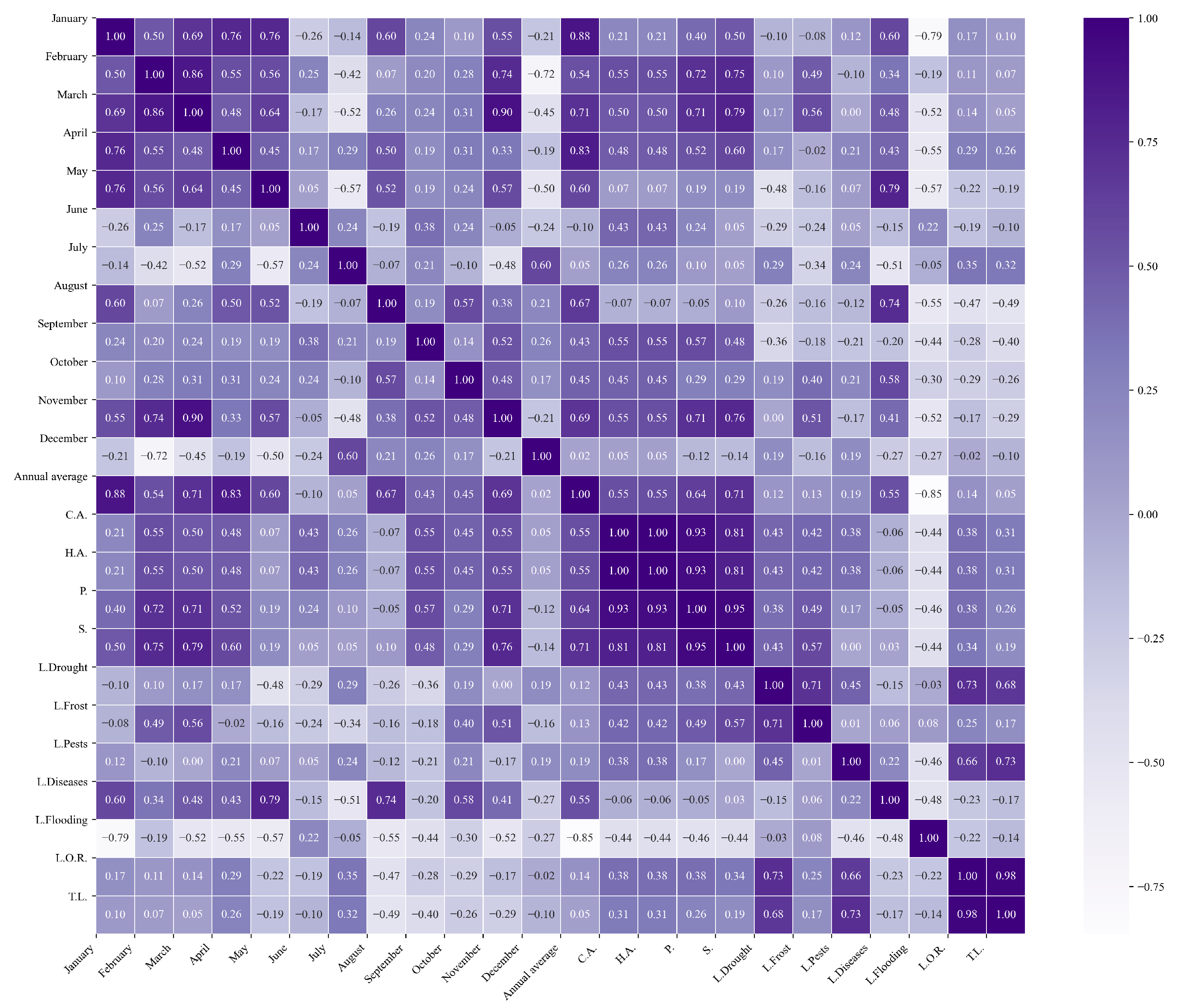
Figure 17 shows the correlations for the central zone. The correlation of $0.9944$ between C.A. and H.A. suggests that almost all the land allocated to cultivation is harvested, reflecting efficient land management. In addition, the strong correlations between C.A. and P. ($0.9315$) and S. ($0.9360$) demonstrate that cultivated area directly influences production and sales. Likewise, H.A. shows a significant correlation with P. ($0.9118$) and S. ($0.9211$), confirming that harvested area impacts the quantity produced and sold. The correlation of $0.9880$ between P. and S. reinforces the expected relationship between production and sales, highlighting that any increase in production translates into higher sales.

On the other hand, a significant correlation of $0.9542$ is observed between L.O.R. and T.L., suggesting that a large portion of total losses is related to non-climatic and non-biological factors, such as logistical or management issues. This finding underscores the need to optimize internal processes and improve infrastructure to reduce losses that are not directly related to environmental conditions. In addition, L.Frost show important correlations with variables such as C.A. ($0.8484$), H.A. ($0.8177$), P. ($0.9191$), and S. ($0.9292$), indicating that frost considerably affects the production and marketing of quinoa. As the scale of production increases, so does exposure to frost risk, highlighting the need to implement climate risk mitigation strategies.

Precipitation also plays a crucial role in agricultural yield. L.Pests shows a correlation of $0.8530$ with January, $0.8955$ with April, and an even higher correlation of $0.9623$ with June, indicating that precipitation conditions in these months are associated with the occurrence of pests that affect the crop. This suggests the need for proactive pest management during these critical months to mitigate the negative impact on production. February precipitation frequently overlaps with the flowering or early reproductive stages in ZC; heavy rains at this time explain the tight link with L.Flooding. Likewise, the January–June rainfall pattern aligns with pest outbreaks favored by high humidity and host tissue availability during the expansion of the canopy leaf area. Likewise, the correlation of $0.9715$ between L.Flooding and February highlights the importance of implementing measures to manage excess water during this period, as heavy rains in February are strongly related to flooding losses.

• Southern zone

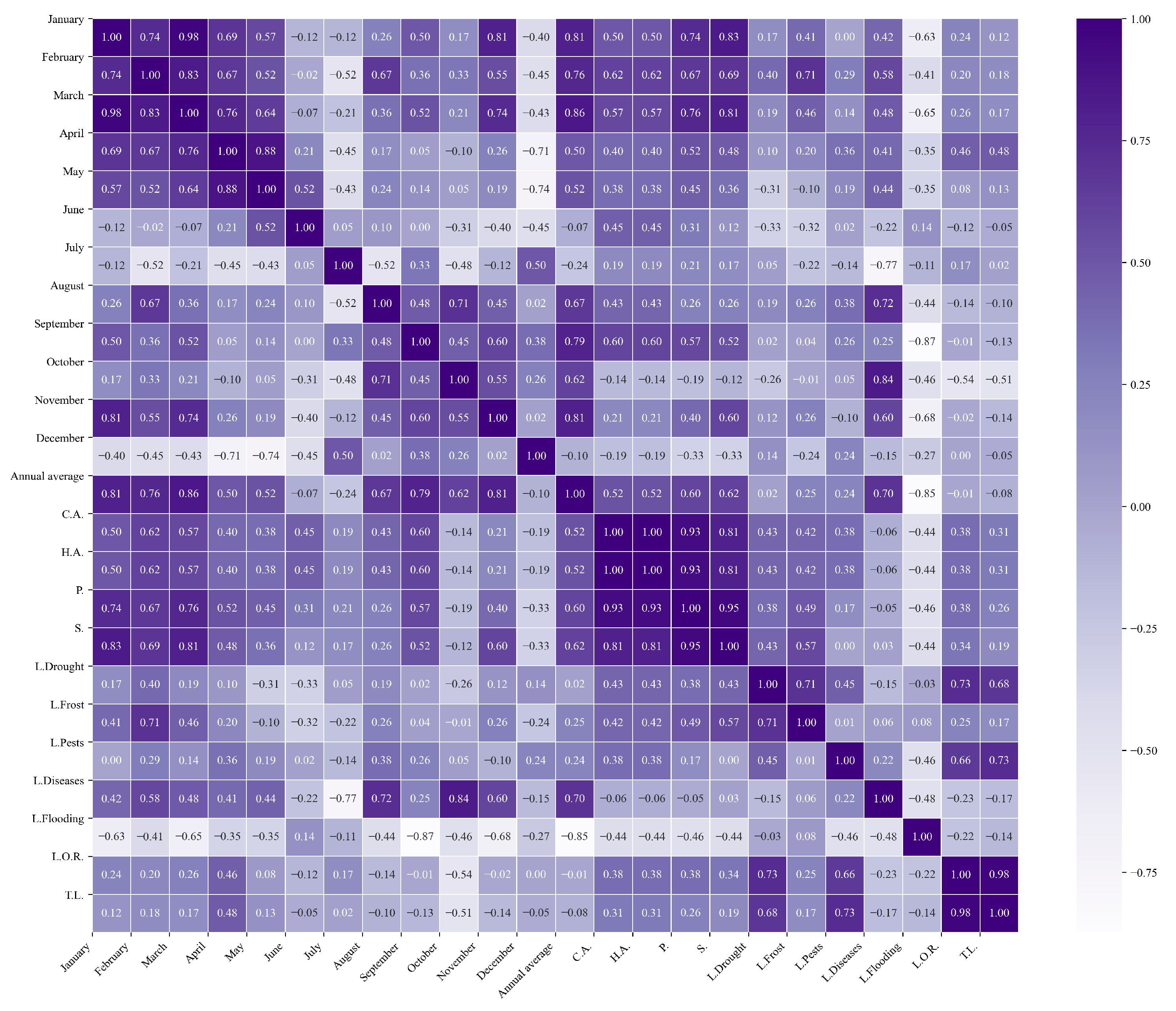
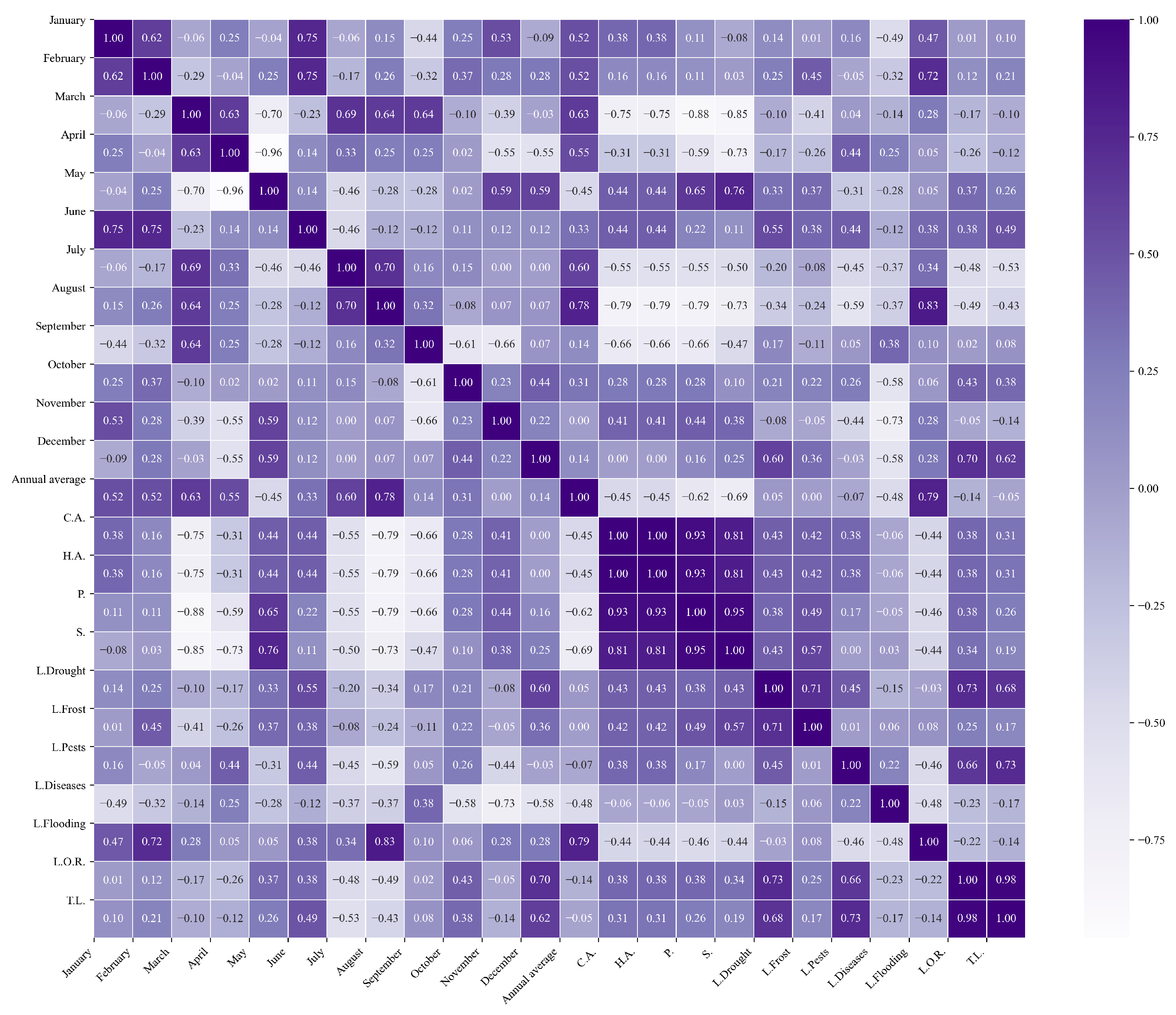
In the southern zone, Figure 18 shows the correlations for this region. Among the most notable is the correlation of $0.9542$ between L.O.R. and T.L. This finding suggests that a large share of total losses in quinoa cultivation is related to non-climatic and non-biological factors, such as logistical or management issues. This correlation reinforces the importance of optimizing internal processes and improving infrastructure to reduce losses that are not directly related to environmental conditions.

On the other hand, L.Frost show significant correlations with various agricultural variables: C.A. ($0.8484$), H.A. ($0.8177$), P. ($0.9191$), and S. ($0.9292$). These correlations indicate that frost has a considerable impact on quinoa production and marketing. As the scale of production increases, so does exposure to frost risk, underscoring the need to implement climate risk mitigation strategies to protect crop yield.

Regarding precipitation, a positive correlation of $0.8685$ is observed between Annual average and March. This indicates that years with higher average precipitation also tend to have higher precipitation in March, which could influence crop growth conditions during this critical phase of the agricultural cycle.

Precipitation is also related to agricultural losses, as observed in the correlations between rainfall and L.Frost. These correlations suggest that climate planning is essential to reduce the impact of frost and optimize production. The correlations between precipitation in different months and agricultural losses underscore the importance of integrated climate management to mitigate risks and maximize yields.

In ZS, March typically sits at the late vegetative–flowering stage; higher seasonal precipitation combined with March peaks improves water status for reproductive initiation, while late-season reductions in rainfall coincide with the decline of flooding losses and favor maturation.

Scope and Limitations

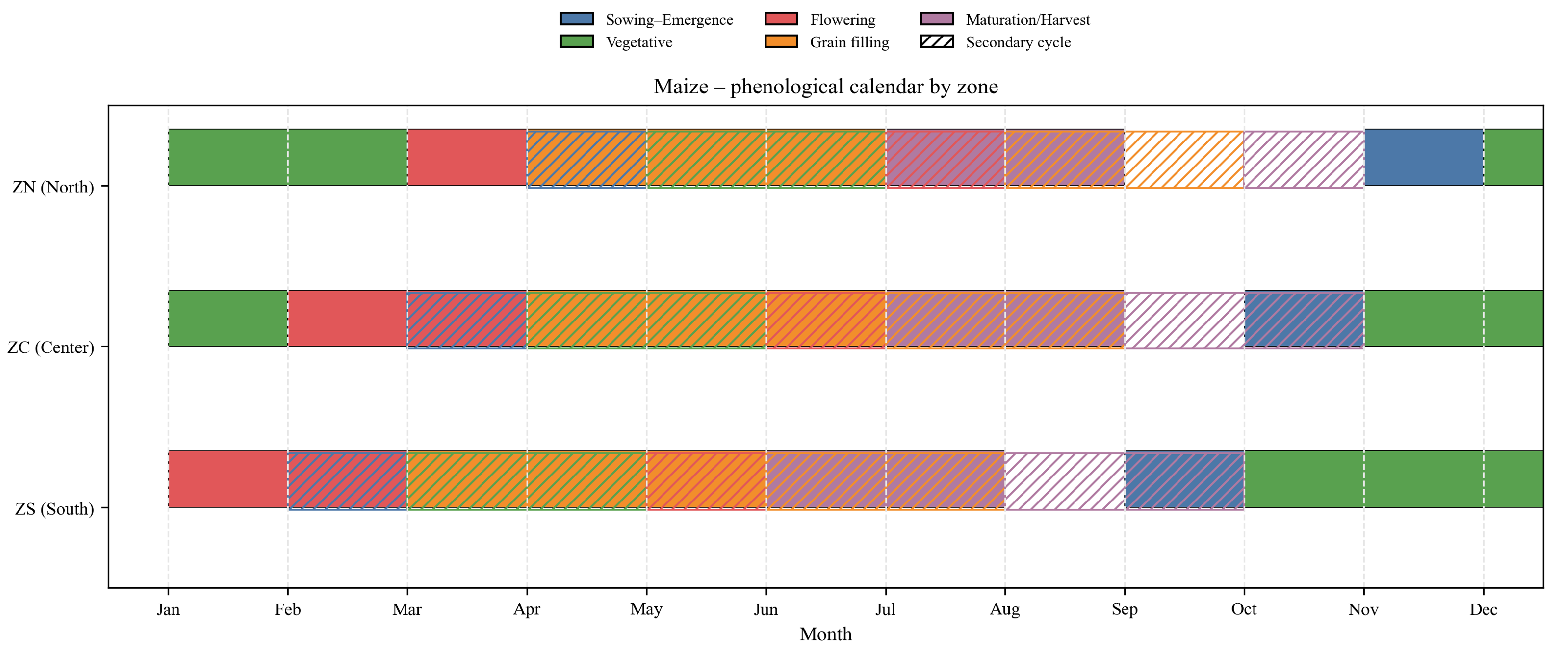
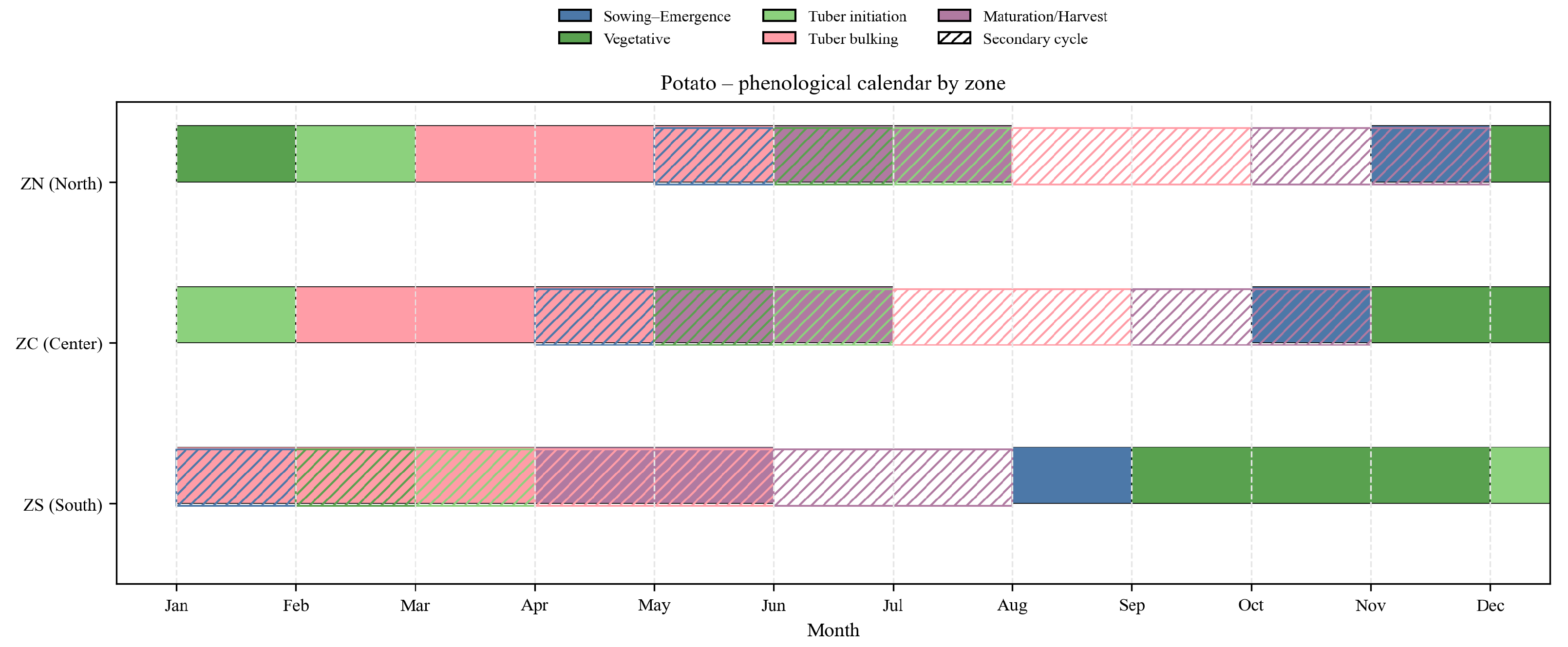
Phenological windows vary with altitude, cultivar, and management (e.g., irrigation), so some plantings depart from the modal calendar. Our interpretation therefore uses zone-specific calendars as a guide (Table A2, Figure A2) and focuses on phase-consistent mechanisms (establishment, flowering, grain filling). These additions provide phenology-based explanations for significant correlations without modifying the statistical procedure or results.

5. Simple Linear Regressions and Multiple Regressions

After identifying the existing correlations among the study variables, we performed linear regressions between pairs of variables to enable a deeper analysis. Based on these regressions and their statistical significance, it is possible to explore and model the relationship between two variables: a dependent (or response) variable and an independent (or predictor) variable.

From this information, we can determine whether it is feasible to generate predictions; that is, by knowing the values of the independent variables, we can estimate the outcomes of the dependent variables. In addition, regressions help identify and understand linear trends in the data, which is useful for making decisions based on historical data or forecasts.

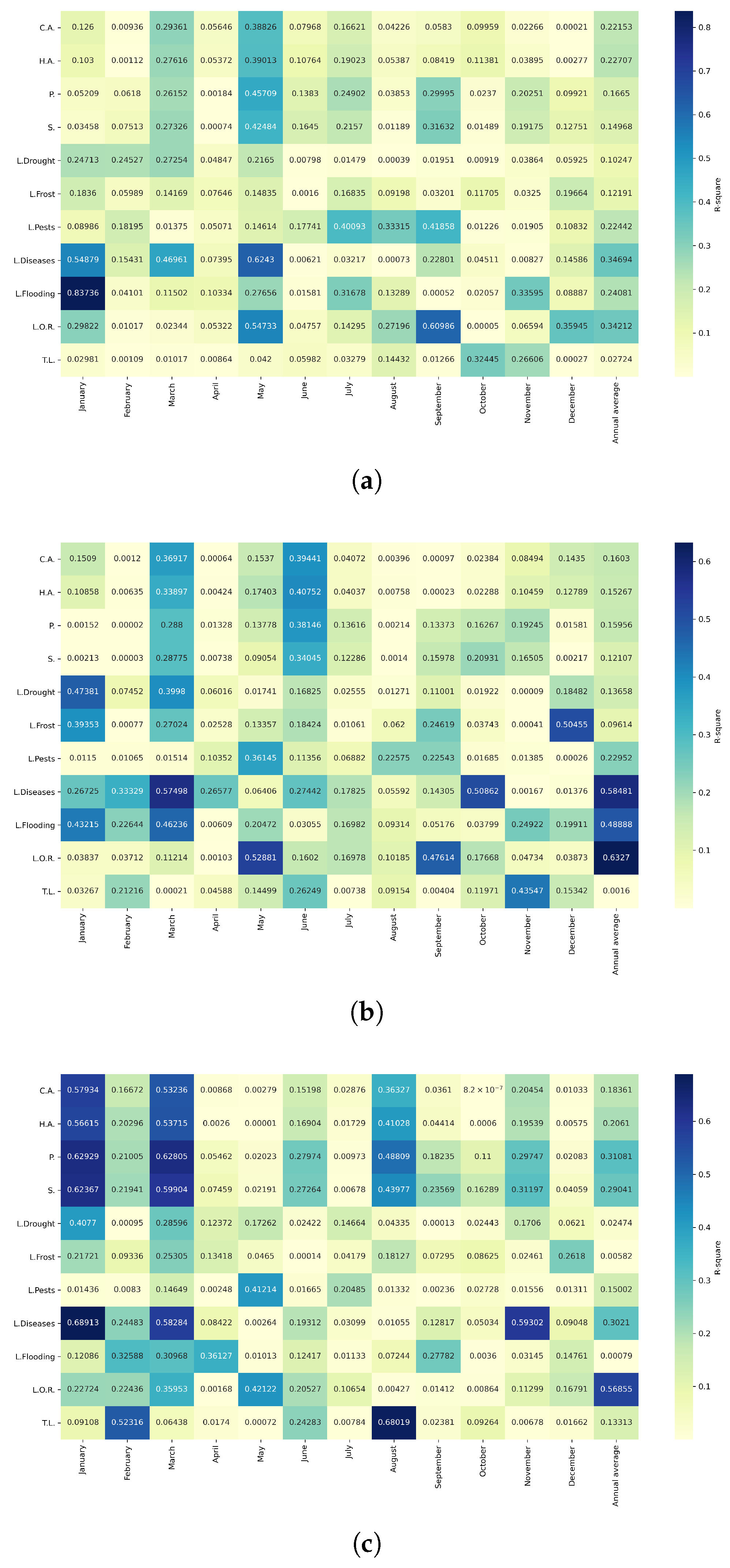
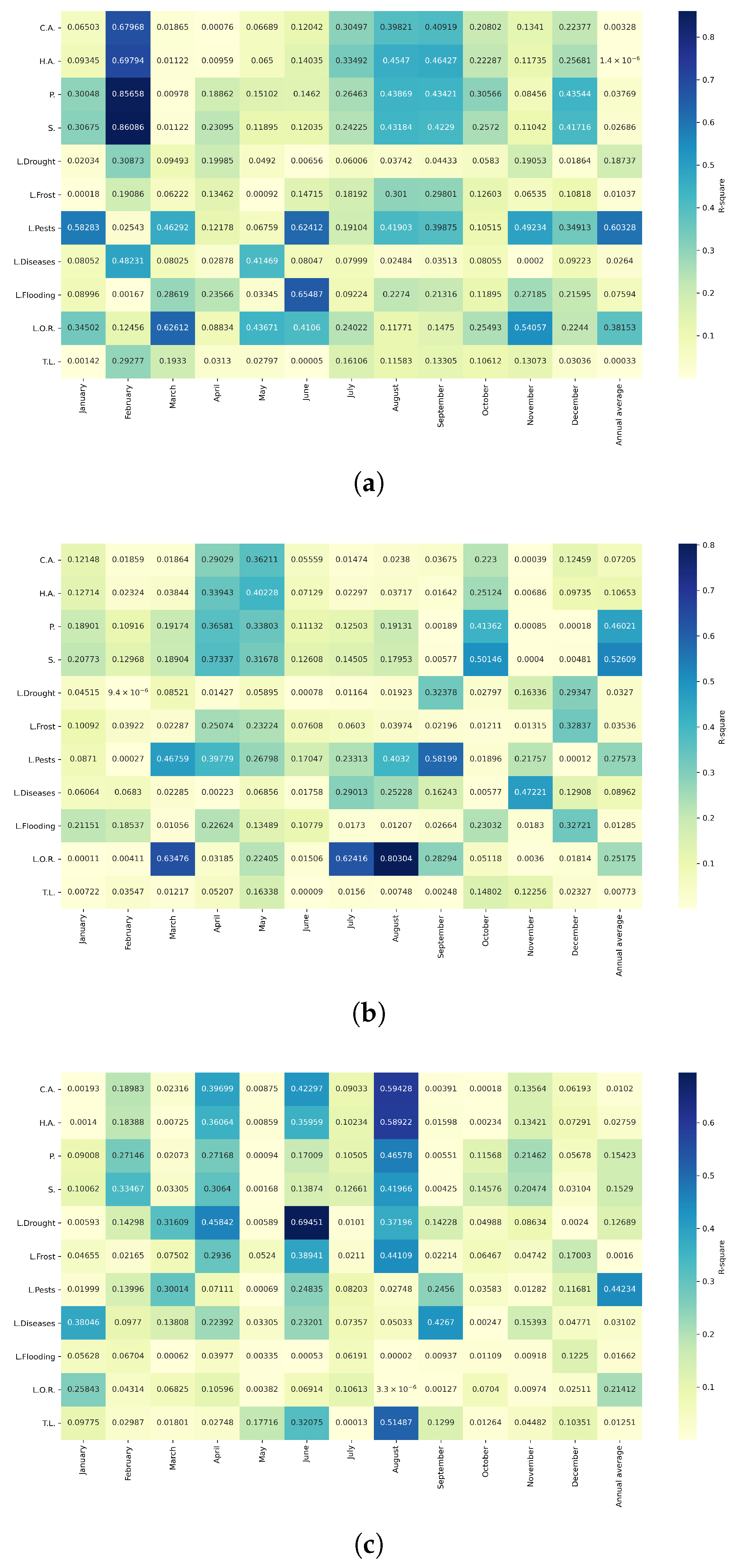
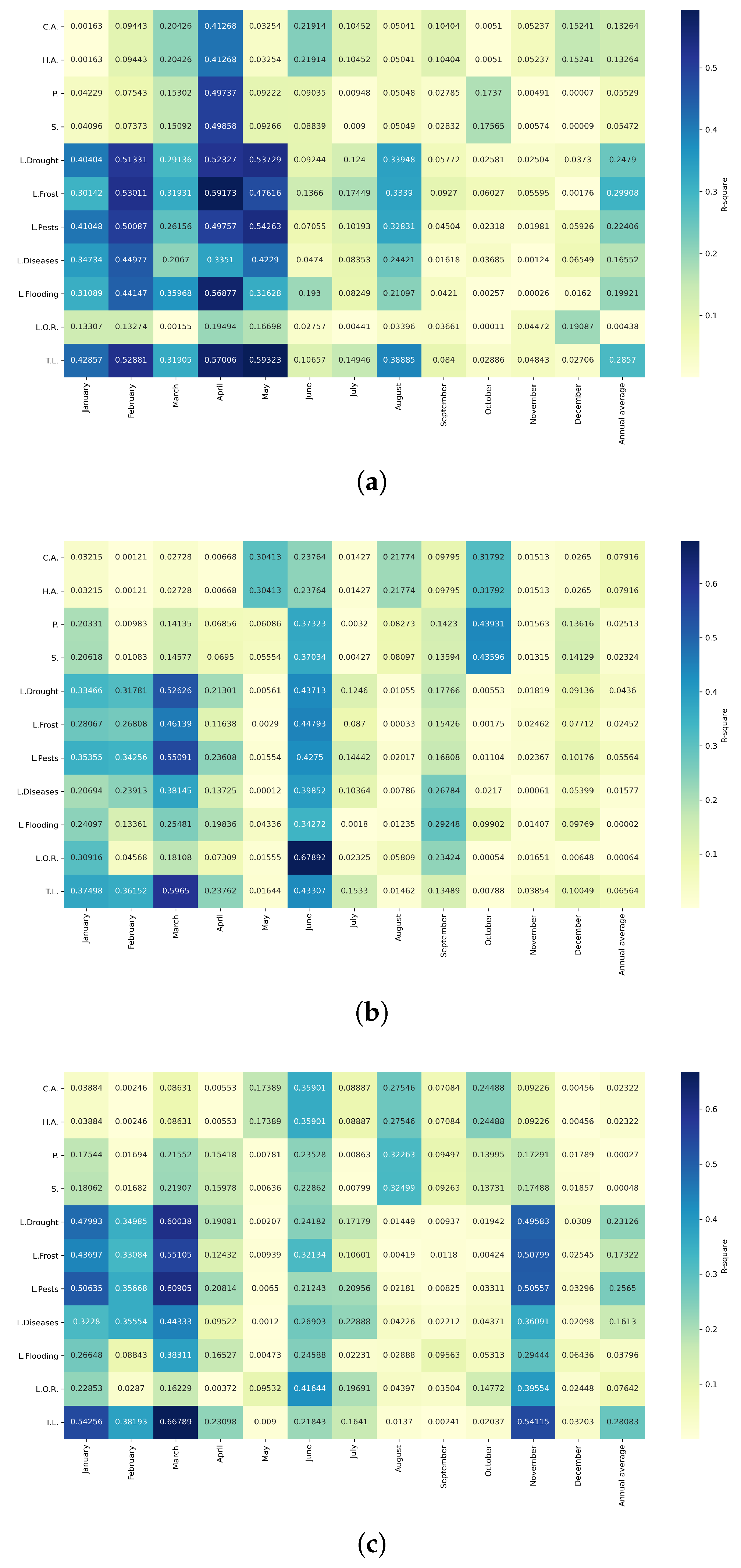
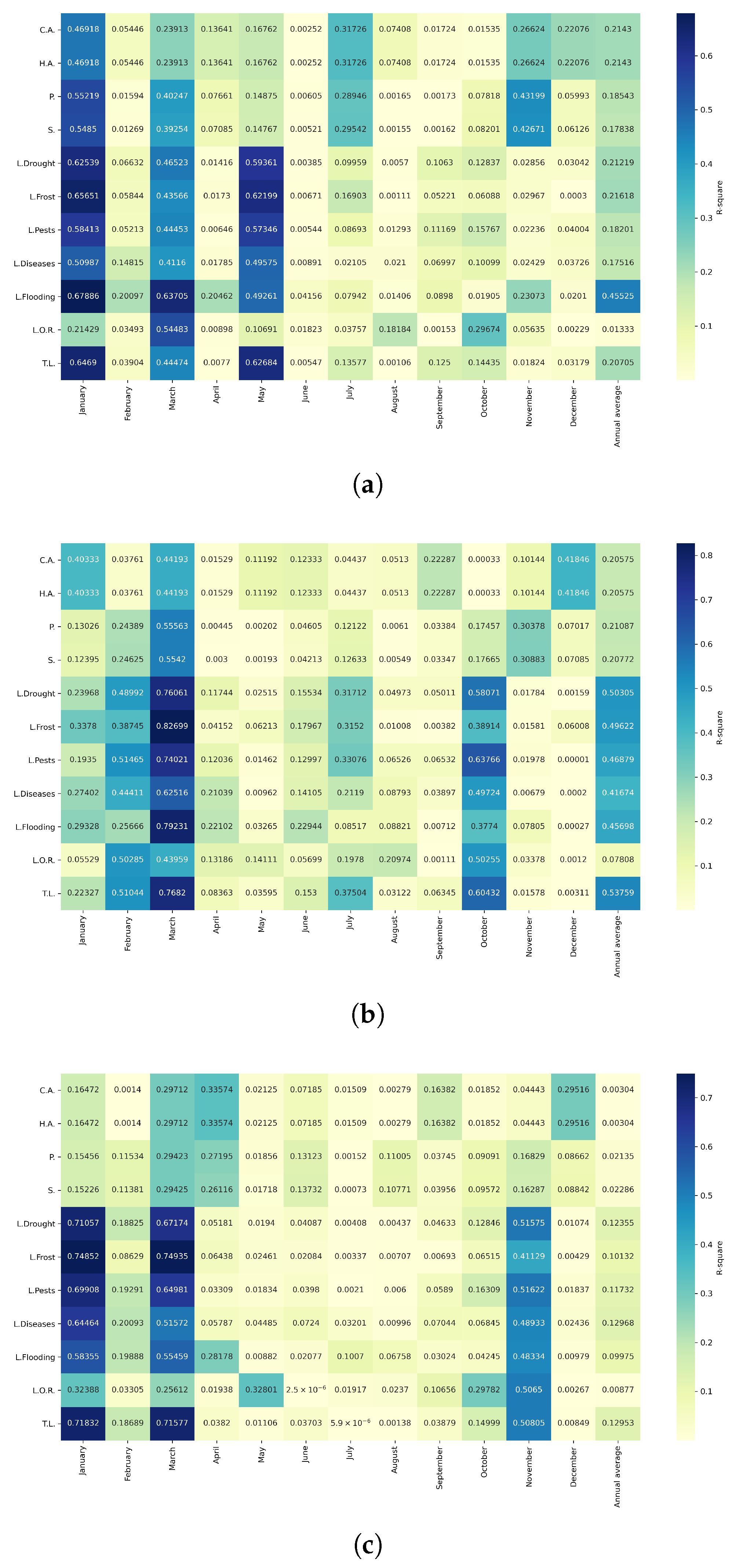
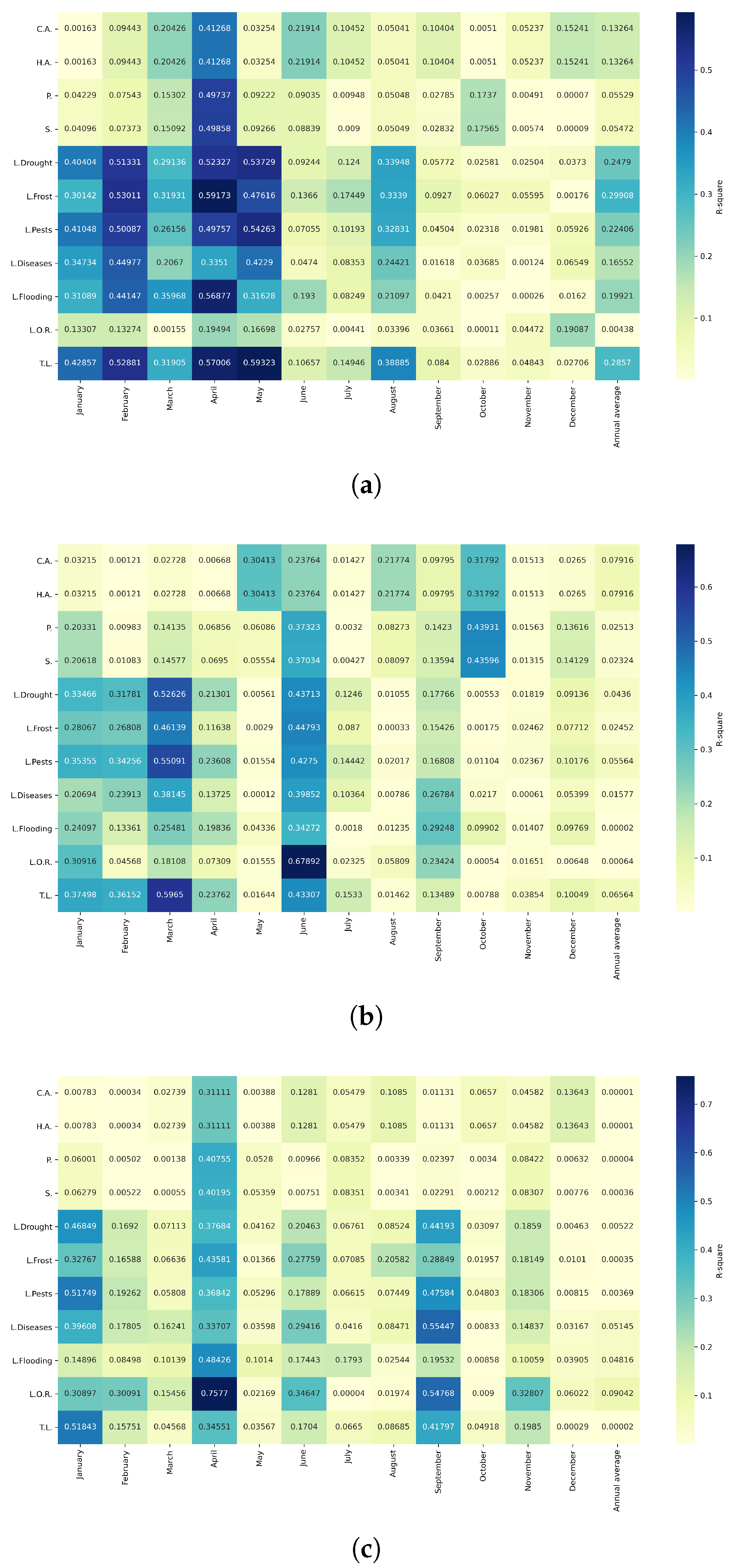
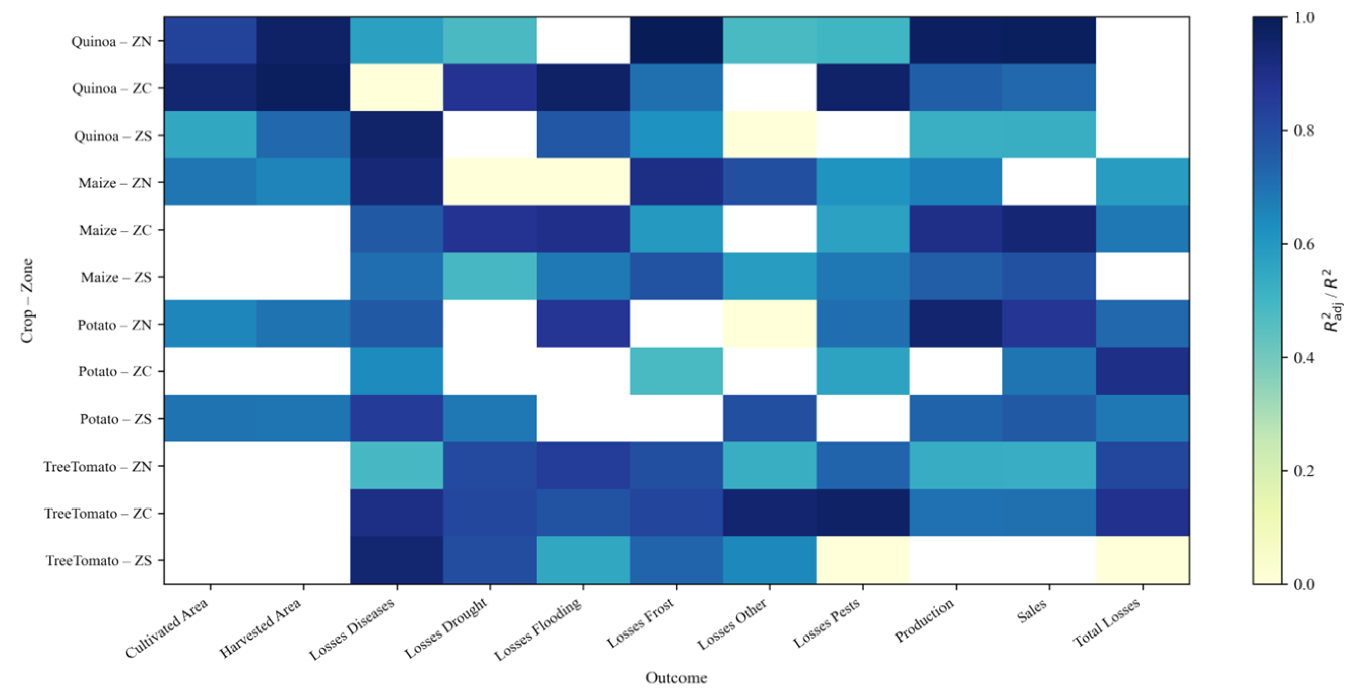
Given the large number of variables under analysis, instead of plotting each simple linear regression considering its regression coefficient, axis intercepts, coefficients of determination ($R^2$), and statistical significance (p-value), we propose generating heatmaps considering only the $R^2$ value to visualize the main variables that could be relevant as predictive equations.

5.1. Heatmaps of $R^2$ Values for the Highland Crop Quinoa

5.1.1. $R^2$ Values in Relation to Monthly Maximum Temperatures

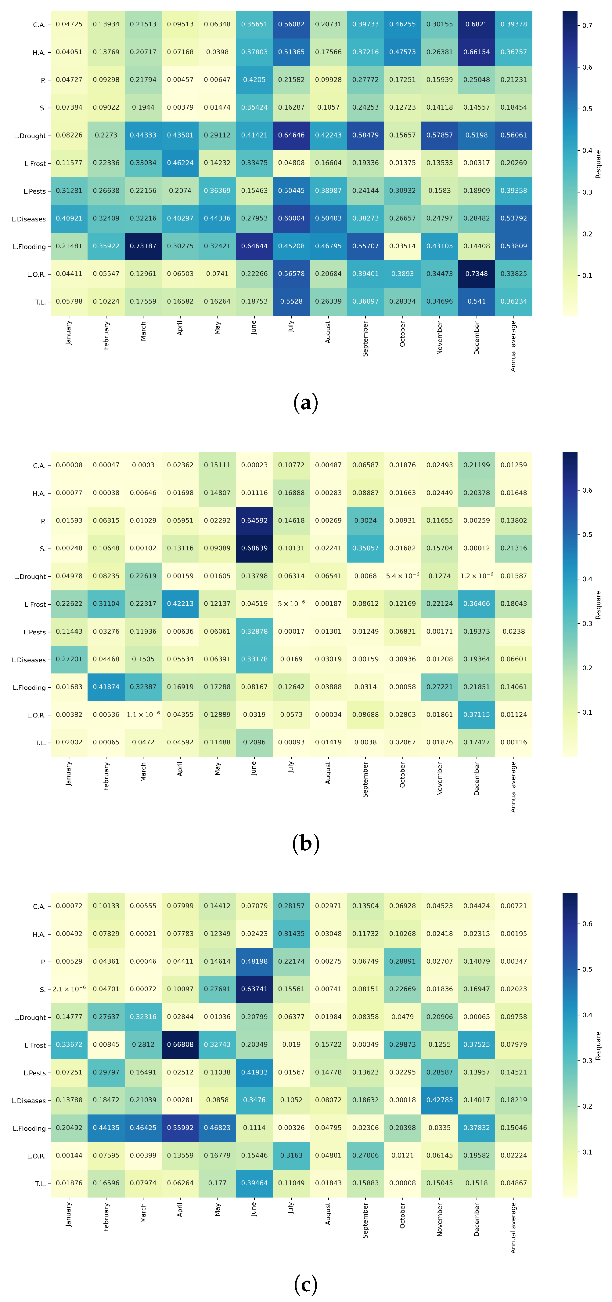
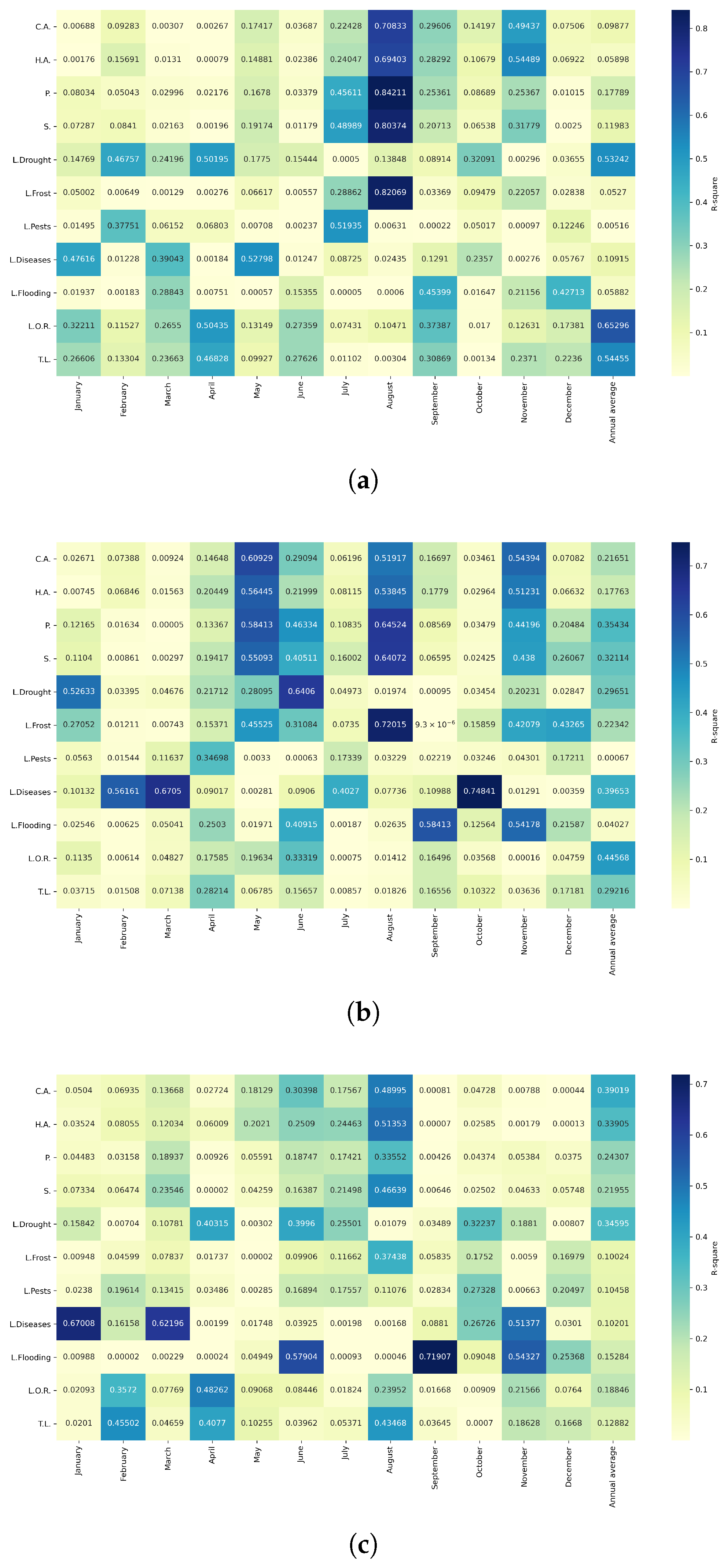
Figure 19 shows the heatmaps of the variables relating monthly maximum temperatures in the three zones with quinoa cultivation.

In the northern zone, Figure 19a, maximum temperature shows highly significant correlations with various quinoa crop variables. L.Diseases show a correlation in May ($R^2$ = 0.58). C.A. has strong correlations with temperatures in July ($R^2$ = 0.76), September ($R^2$ = 0.74), November ($R^2$ = 0.73), and December ($R^2$ = 0.63), as well as with the annual average ($R^2$ = 0.61). H.A. also presents significant correlations, especially in November ($R^2$ = 0.76). P. and S. are highly correlated with temperatures across several months, with July, September, November, and December standing out, reaching $R^2$ values of up to $0.86$ for production and $0.84$ for sales. Finally, L.Frost show a strong relationship with temperatures in July ($R^2$ = 0.67) and December ($R^2$ = 0.85). These results underscore the importance of maximum temperatures in yield performance and risk management for quinoa cultivation in the northern zone.

In the central zone, Figure 19b, maximum temperature shows significant correlations with various quinoa crop variables. L.Diseases show a correlation with maximum temperatures in March ($R^2$ = 0.63), suggesting that high temperatures in this month influence the incidence of diseases. In addition, H.A. presents a significant correlation with temperatures in September ($R^2$ = 0.57), indicating that temperatures in this month have an impact on the amount of harvested area. These relationships highlight the influence of maximum temperatures on key aspects of quinoa production in the central zone.

In the southern zone, Figure 19c, maximum temperature shows significant correlations with various quinoa crop variables. L.Diseases present significant correlations with temperatures in January ($R^2$ = 0.59), March ($R^2$ = 0.64), and November ($R^2$ = 0.57), suggesting that high temperatures in these months influence the incidence of diseases. In September, C.A., H.A., P., and S. all present significant correlations with temperatures, with $R^2$ values ranging from $0.54$ to $0.61$, highlighting the impact of temperatures on the yield and marketing of quinoa in the southern zone.

5.1.2. $R^2$ Values in Relation to Monthly Minimum Temperatures

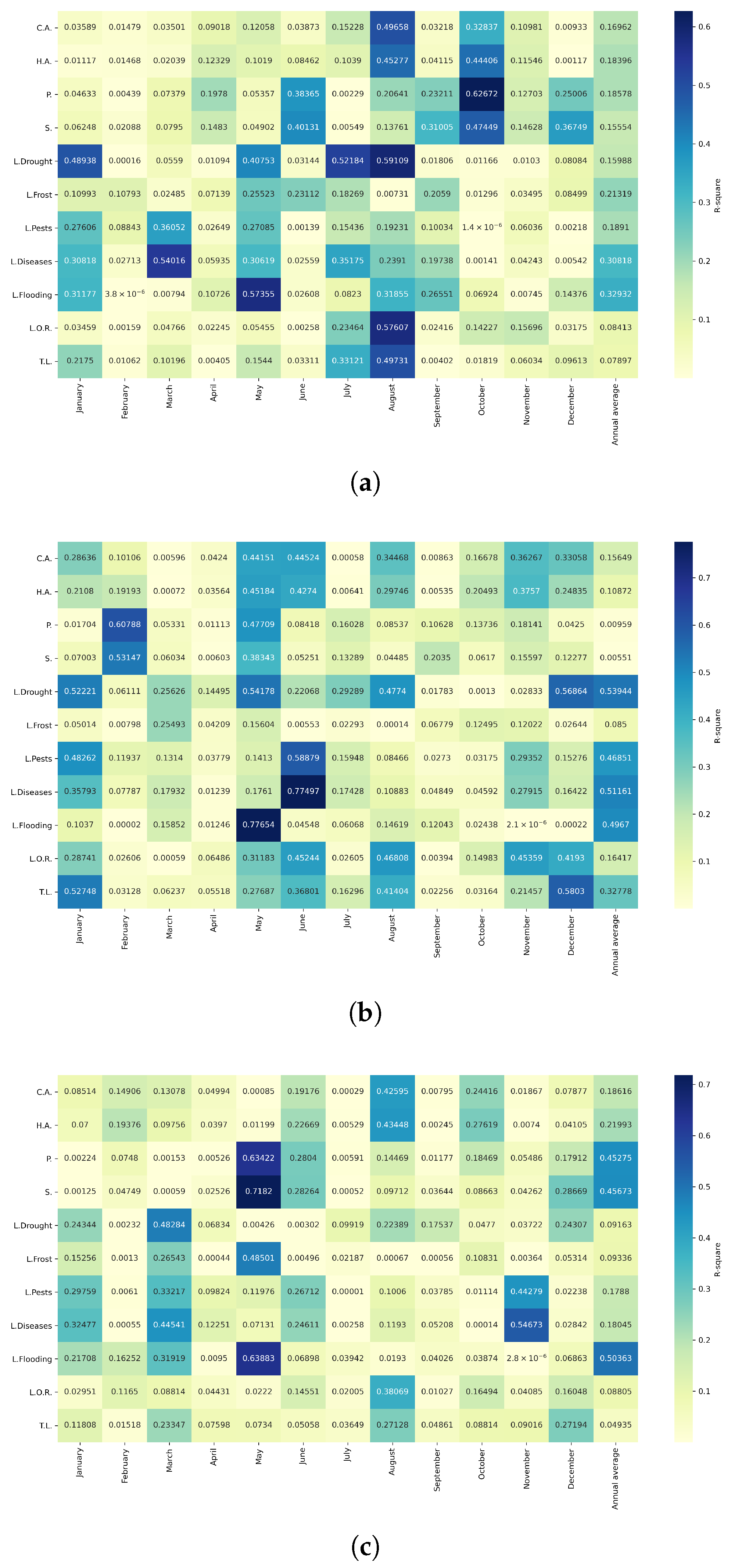
Figure 20 shows the heatmaps of the variables relating monthly minimum temperatures in the three zones with quinoa cultivation.

In the northern zone, as shown in Figure 20a, minimum temperature shows significant correlations with various agricultural variables related to quinoa cultivation throughout the year. L.Drought and L.O.R. are correlated with minimum temperatures in April and with the annual average, with $R^2$ values reaching up to $0.65$ for L.O.R. in the annual average. L.Diseases and L.Pests show correlations in May and July, respectively. In August, strong correlations are observed with C.A., H.A., P., S., and L.Frost, with $R^2$ values above 0.70, highlighting the impact of minimum temperatures on productivity and risk management during this month. Finally, T.L. are also correlated with the annual average of minimum temperatures ($R^2$ = 0.54), underscoring the influence of low temperatures on the overall yield of quinoa cultivation in the northern zone.

In the central zone, as shown in Figure 20b, minimum temperature shows significant correlations with different variables of quinoa cultivation throughout the year. Losses due to drought (L.Drought) are correlated with minimum temperatures in January ($R^2$ = 0.53) and June ($R^2$ = 0.64), suggesting that low temperatures in these months affect drought risk. L.Diseases show high correlations in February ($R^2$ = 0.56), March ($R^2$ = 0.67), and October ($R^2$ = 0.75). In May, a significant correlation is observed with C.A., H.A., P., and S., with $R^2$ values ranging from $0.55$ to $0.61$. August also shows notable correlations with these same variables and L.Frost, reaching $R^2$ = 0.72 for L.Frost. Finally, L.Flooding are correlated in September ($R^2$ = 0.58) and November ($R^2$ = 0.54), underscoring the influence of minimum temperatures on risk management and quinoa crop productivity in the central zone.

In the southern zone, Figure 20c, minimum temperature shows significant correlations with several critical variables of quinoa cultivation throughout the year. L.Diseases is highly correlated with minimum temperatures in January ($R^2$ = 0.67), March ($R^2$ = 0.62), and November ($R^2$ = 0.51), suggesting that low temperatures in these months affect disease incidence. L.Flooding shows strong correlations in June ($R^2$ = 0.58), September ($R^2$ = 0.72), and November ($R^2$ = 0.54), highlighting the influence of low temperatures on flood risk. Additionally, H.A. shows a significant correlation with minimum temperatures in August ($R^2$ = 0.51), underscoring the impact of temperatures on the amount of harvested area in the southern zone.

5.1.3. $R^2$ Values in Relation to Average Monthly Precipitation

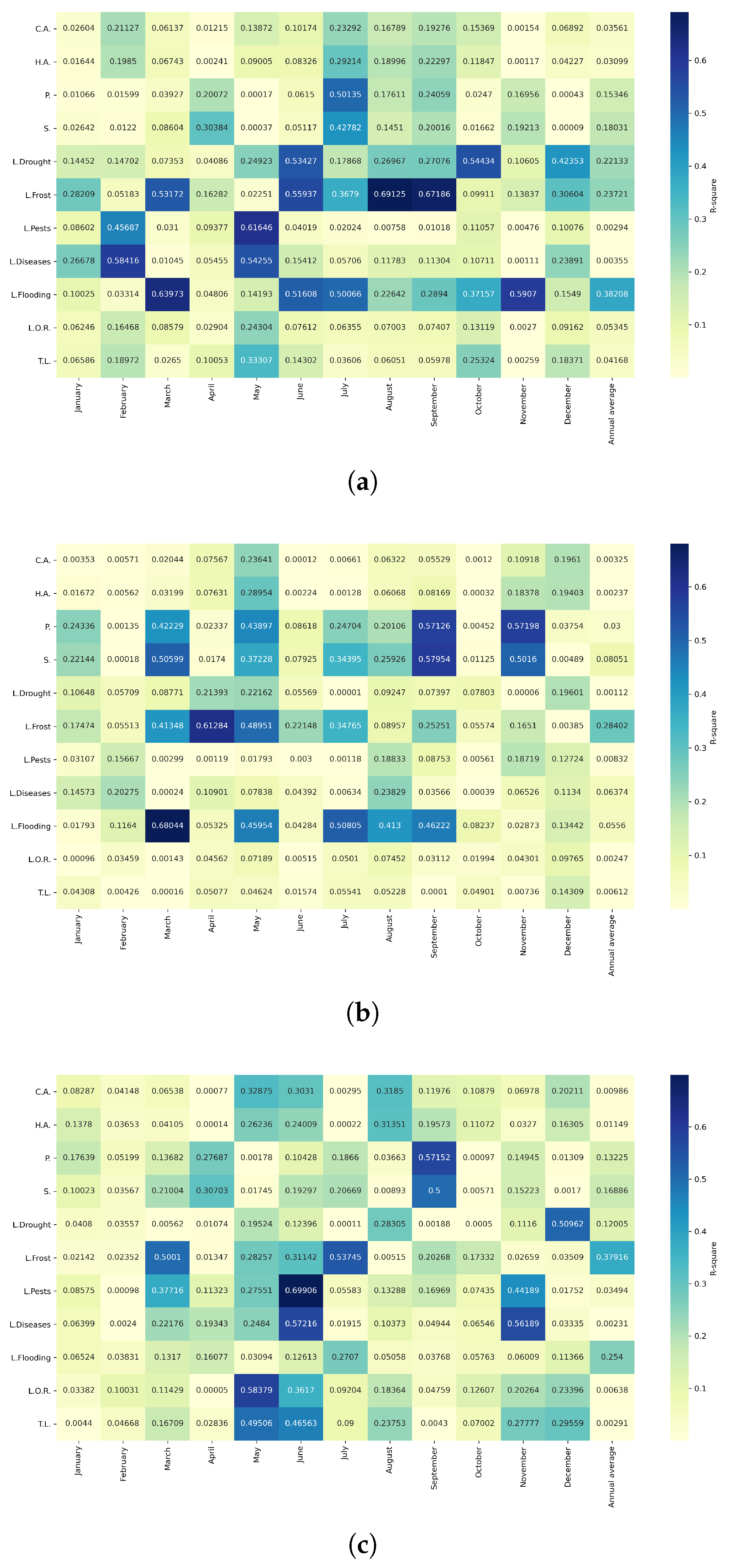
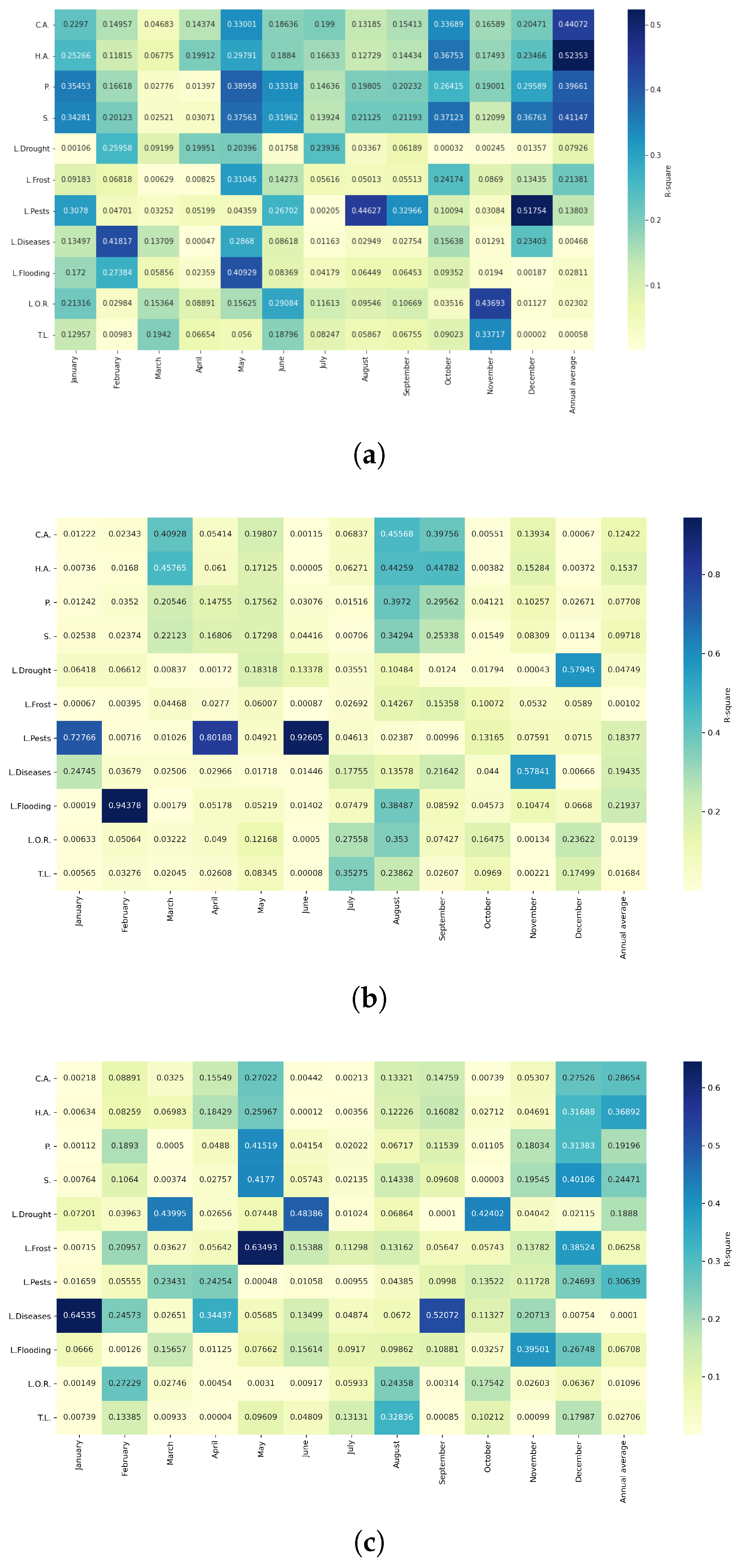
In Figure 21, the heatmaps show the variables relating average monthly precipitation in the three zones to quinoa cultivation.

In the northern zone, as shown in Figure 21a, average precipitation shows significant correlations with various quinoa cultivation variables. Losses due to pests (L.Pests) are correlated with precipitation in December ($R^2$ = 0.52), suggesting that rainfall in this month may influence pest incidence. In addition, H.A. shows a correlation with the annual average precipitation ($R^2$ = 0.52), highlighting the influence of rainfall on the amount of harvested area throughout the year in the northern zone.

In the central zone, as shown in Figure 21b, average precipitation shows significant correlations with various quinoa crop variables. L.Pests exhibit a strong correlation with precipitation in January ($R^2$ = 0.73), April ($R^2$ = 0.80), and June ($R^2$ = 0.93), suggesting that rainfall during these months strongly influences pest incidence. Losses due to flooding (L.Flooding) are highly correlated with precipitation in February ($R^2$ = 0.94), highlighting the risk of flooding during this month. Additionally, L.Diseases and L.Drought are correlated with precipitation in November ($R^2$ = 0.58) and December ($R^2$ = 0.58), respectively, underscoring the influence of rainfall on agricultural risk management in the central zone.

In the southern zone, as shown in Figure 21c, average precipitation is also significantly related to several key quinoa crop variables. L.Diseases shows a significant correlation with precipitation in January ($R^2$ = 0.65) and September ($R^2$ = 0.52), suggesting that rainfall in these months may influence disease incidence. Moreover, L.Frost presents a correlation with precipitation in May ($R^2$ = 0.63), highlighting the impact of rainfall on frost risk during that month in the southern zone.

5.2. Multiple Linear Regressions

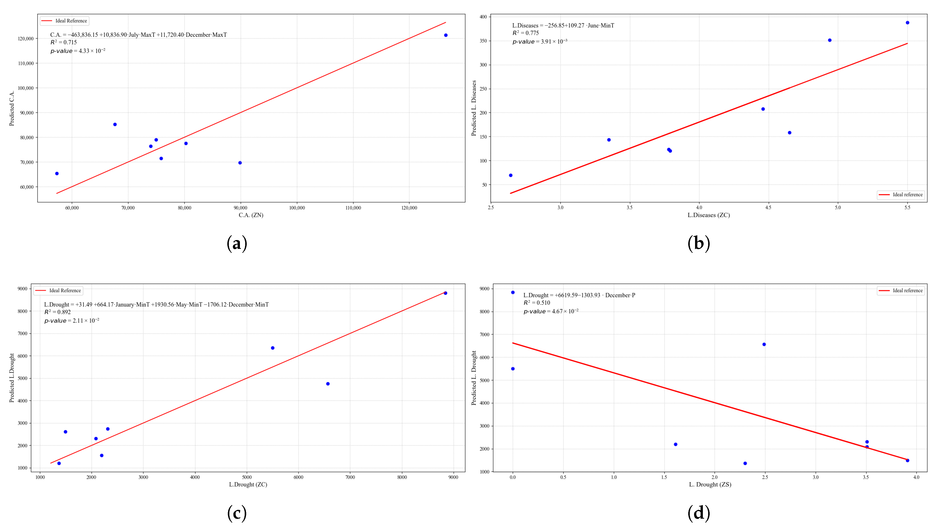
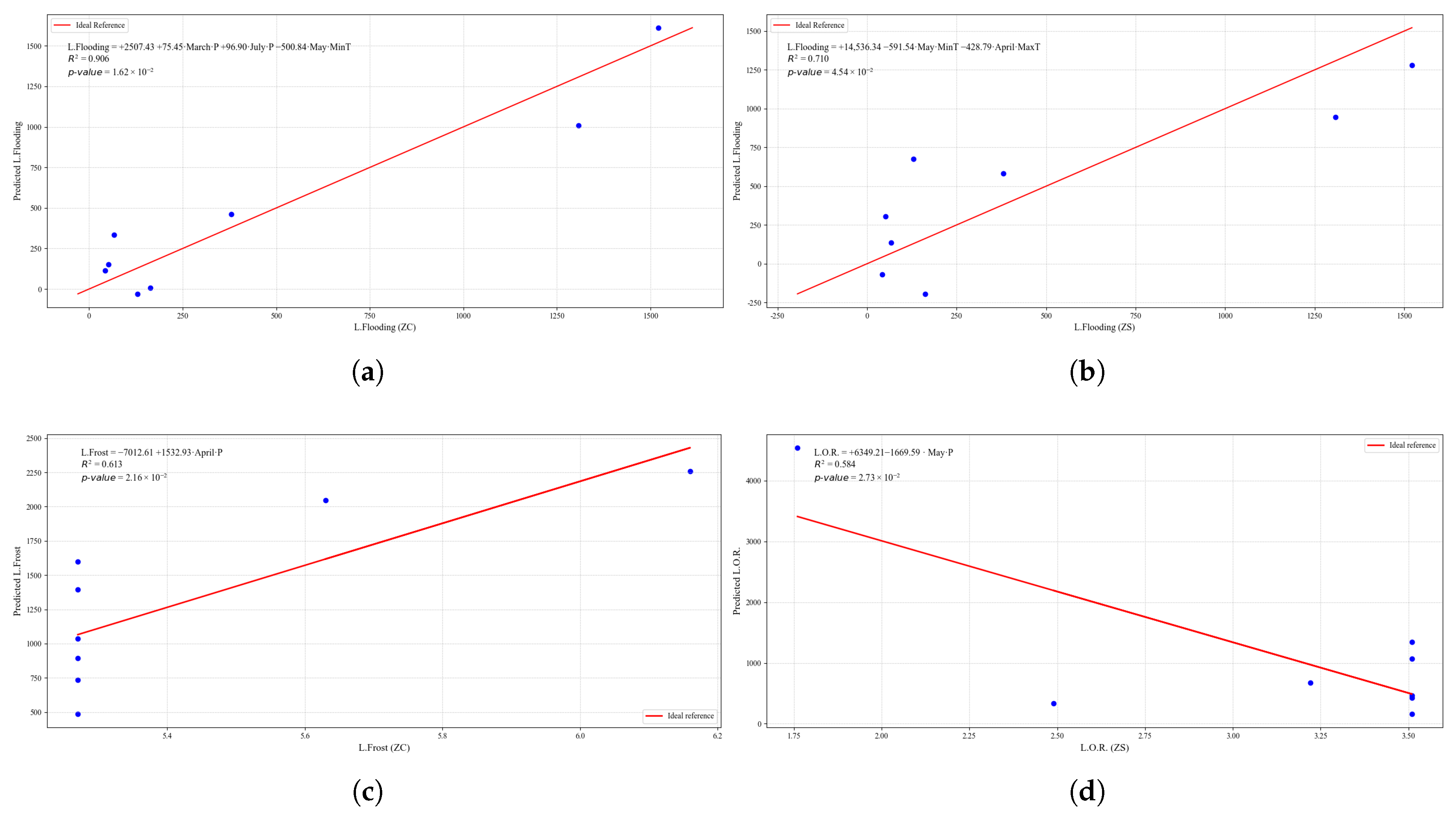
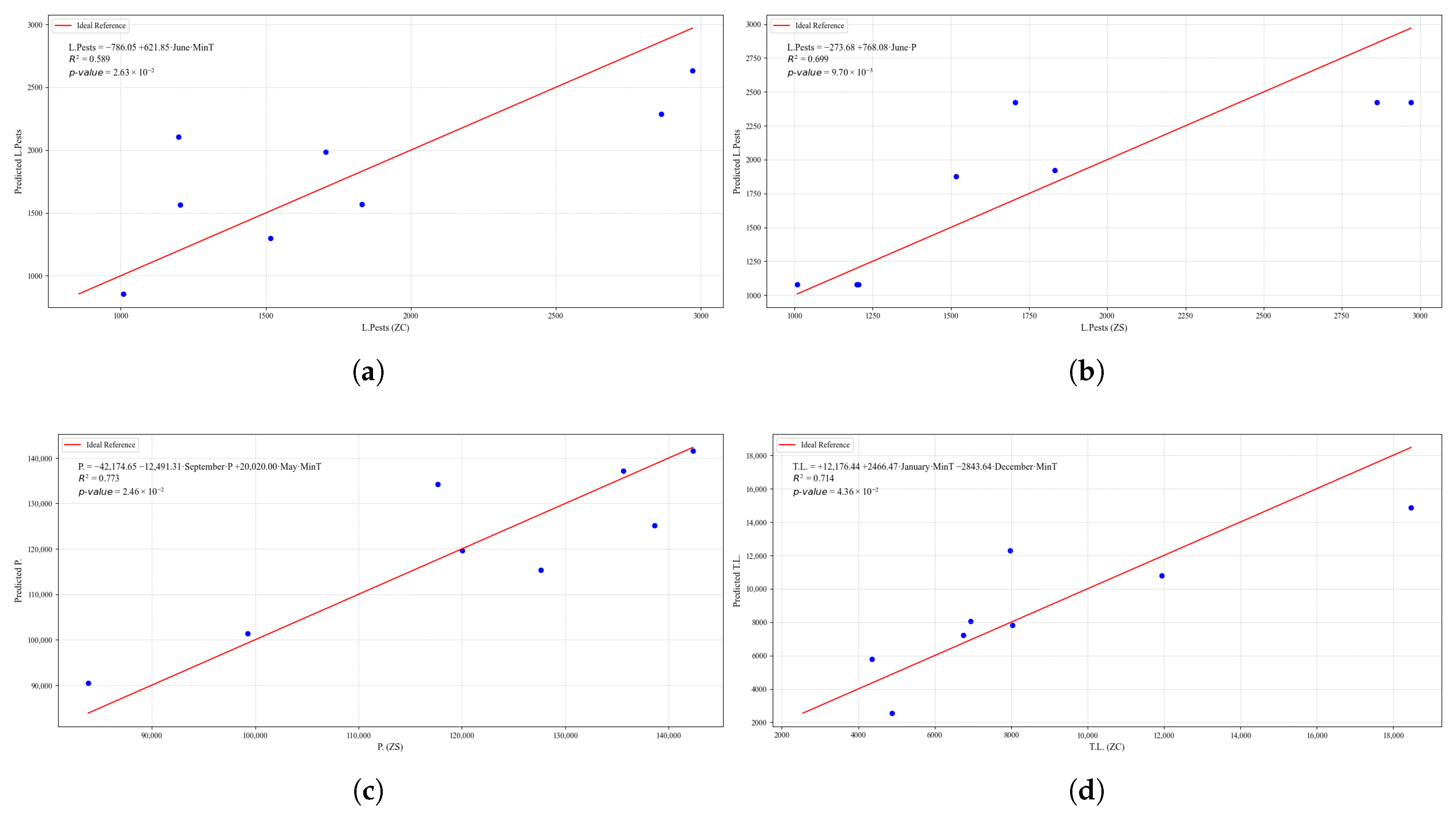
To deepen the understanding of the relationships identified between climatic variables and critical aspects of the high-Andean crops studied, a multiple linear regression analysis was conducted using the $R^2$ values greater than 0.5 obtained from the previous correlations. This approach allows us to quantify the impact of multiple independent variables (such as maximum temperatures and precipitation) on a specific dependent variable, such as production, cultivated area, or pest and disease management. By employing multiple linear regressions, it is possible not only to identify the individual influence of each climatic variable but also to assess how these variables interact jointly to affect agricultural outcomes in the different study zones. This analysis provides a more robust quantitative basis for planning and decision-making in crop management, enabling the development of more precise and effective strategies to mitigate adverse climate effects and optimize agricultural productivity.

5.2.1. Multiple Linear Regressions for Quinoa Cultivation

Table 17. Summary of multiple linear regression models for different dependent variables. The table presents the equations used, along with the corresponding $R^2$ and p-values, indicating the strength and statistical significance of each model. The results allow for the evaluation of the relationship between climatic variables and quinoa crop characteristics.

Variable	Equations	${\mathit{R}}^2$	p-Value	${\mathit{R}}_{\mathbf{adj}}^2$	AICc	LOYO MSE	VIFmax
C.A.	[(‘July’, ‘MaxTempZN’), (‘August’, ‘MaxTempZN, MinTempZN’), (‘September’, ‘MaxTempZN’), (‘November’, ‘MaxTempZN’), (‘December’, ‘MaxTempZN’)]	0.872	0.614	0.83	149.84	$6.4\times {10}^8$	123.54
	[(‘May’, ‘MinTempZC’), (‘August’, ‘MinTempZC’), (‘November’, ‘MinTempZC’)]	0.953	0.0040	0.946	130.9	$1.2\times {10}^6$	1.67
	[(‘September’, ‘MaxTempZS’)]	0.567	0.0310	0.547	143.21	$3.9\times {10}^6$	1
H.A.	[(‘July’, ‘MaxTempZN’), (‘August’, ‘MinTempZN’), (‘September’, ‘MaxTempZN’), (‘November’, ‘MaxTempZN, MinTempZN’), (‘December’, ‘MaxTempZN’)]	0.977	0.279	0.969	135.46	$3.1\times {10}^7$	41.43
	[(‘May’, ‘MinTempZC’), (‘August’, ‘MinTempZC’), (‘September’, ‘MaxTempZC’), (‘November’, ‘MinTempZC’)]	0.986	0.00389	0.984	123.59	$7.3\times {10}^5$	1.91
	[(‘August’, ‘MinTempZS’), (‘September’, ‘MaxTempZS’)]	0.749	0.0314	0.726	140.82	$3.1\times {10}^6$	1.34
P.	[(‘July’, ‘MaxTempZN’), (‘August’, ‘MaxTempZN, MinTempZN’), (‘September’, ‘MaxTempZN’), (‘November’, ‘MaxTempZN’), (‘December’, ‘MaxTempZN’)]	0.982	0.243	0.977	142.21	$2.4\times {10}^8$	123.43
	[(‘May’, ‘MinTempZC’), (‘August’, ‘MinTempZC’)]	0.769	0.0256	0.747	149.19	$1.2\times {10}^7$	1.56
	[(‘September’, ‘MaxTempZS’)]	0.541	0.0376	0.520	152.07	$1.4\times {10}^7$	1
S.	[(‘July’, ‘MaxTempZN’), (‘August’, ‘MaxTempZN, MinTempZN’), (‘September’, ‘MaxTempZN’), (‘November’, ‘MaxTempZN’), (‘December’, ‘MaxTempZN’)]	0.991	0.176	0.988	134.52	$9.5\times {10}^7$	123.54
	[(‘May’, ‘MinTempZC’), (‘August’, ‘MinTempZC’)]	0.747	0.0320	0.723	147.42	$9.03\times {10}^6$	1.56
	[(‘September’, ‘MaxTempZS’)]	0.547	0.0359	0.527	149.47	$1.03\times {10}^7$	1
T.L.	—	—	—	—	—	—	—
	—	—	—	—	—	—	—
	—	—	—	—	—	—	—
L.Drought	[(‘April’, ‘MinTempZN’)]	0.501	0.917	0.479	109.15	$5.1\times {10}^4$	1
	[(‘January’, ‘MinTempZC’), (‘June’, ‘MinTempZC’), (‘December’, ‘PrecipitationZC’)]	0.892	0.0208	0.877	102.41	$1.9\times {10}^4$	2.95
	—	—	—	—	—	—	—
L.Frost	[(‘July’, ‘MaxTempZN’), (‘August’, ‘MinTempZN’), (‘September’, ‘MaxTempZN’), (‘November’, ‘MaxTempZN’), (‘December’, ‘MaxTempZN’)]	0.998	0.00355	0.998	69.13	664.52	27.21
	[(‘August’, ‘MinTempZC’)]	0.720	0.00772	0.707	99.02	$3.7\times {10}^4$	1
	[(‘May’, ‘PrecipitationZS’)]	0.634	0.0179	0.618	101.15	$5.1\times {10}^4$	1
L.Pests	[(‘July’, ‘MinTempZN’), (‘December’, ‘PrecipitationZN’)]	0.542	0.142	0.499	101.70	$3.6\times {10}^4$	5.97
	[(’January’, ’PrecipitationZC’), (’April’, ’PrecipitationZC’), (’June’, ’PrecipitationZC’)]	0.968	0.00184	0.964	83.19	$6.5\times {10}^4$	8.47
	—	—	—	—	—	—	—
L.Diseases	[(‘May’, ‘MaxTempZN, MinTempZN’)]	0.608	0.907	0.571	94.52	$2.09\times {10}^4$	3.23
	[(‘January’, ‘MaxTempZC, MinTempZC, PrecipitationZC’), (‘February’, ‘MinTempZC’), (‘March’, ‘MinTempZC, PrecipitationZC’), (‘October’, ‘MinTempZC’), (‘November’, ‘PrecipitationZC’)]	1.000	0	0	0	0	0
	[(‘March’, ‘MaxTempZS, MinTempZS’), (‘September’, ‘PrecipitationZS’), (‘November’, ’MaxTempZS, MinTempZS’)]	0.990	0.316	0.96	84.01	$1.3\times {10}^4$	8.73
L.Flooding	—	—	—	—	—	—	—
	[(‘February’, ‘PrecipitationZC’), (‘September’, ‘MinTempZC’), (‘November’, ‘MinTempZC’)]	0.973	0.128	0.97	56.94	524.2	2.51
	[(‘June’, ‘MinTempZS’), (‘September’, ‘MinTempZS’), (‘November’, ‘MinTempZS’)]	0.798	0.750	0.768	73.31	$1.7\times {10}^3$	2.95
L.O.R.	[(‘April’, ‘MinTempZN’)]	0.504	0.0484	0.482	95.96	$1.17\times {10}^4$	1
	—	—	—	—	—	—	—
	[(‘May’, ‘PrecipitationZS’)]	0.003	0.896	-0.042	101.56	$2.1\times {10}^4$	1

presents a summary of the multiple linear regressions for each dependent variable related to quinoa cultivation.

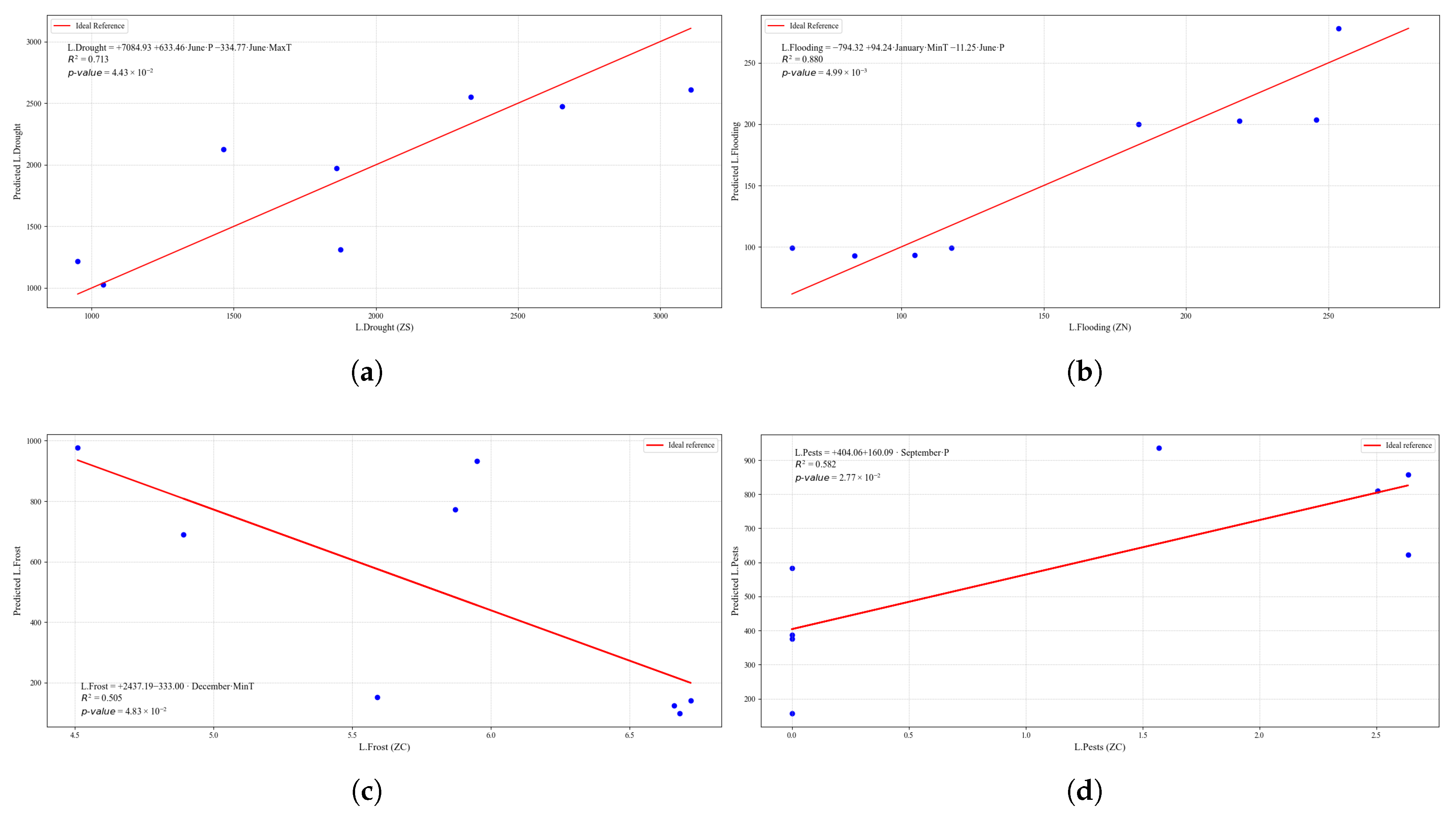
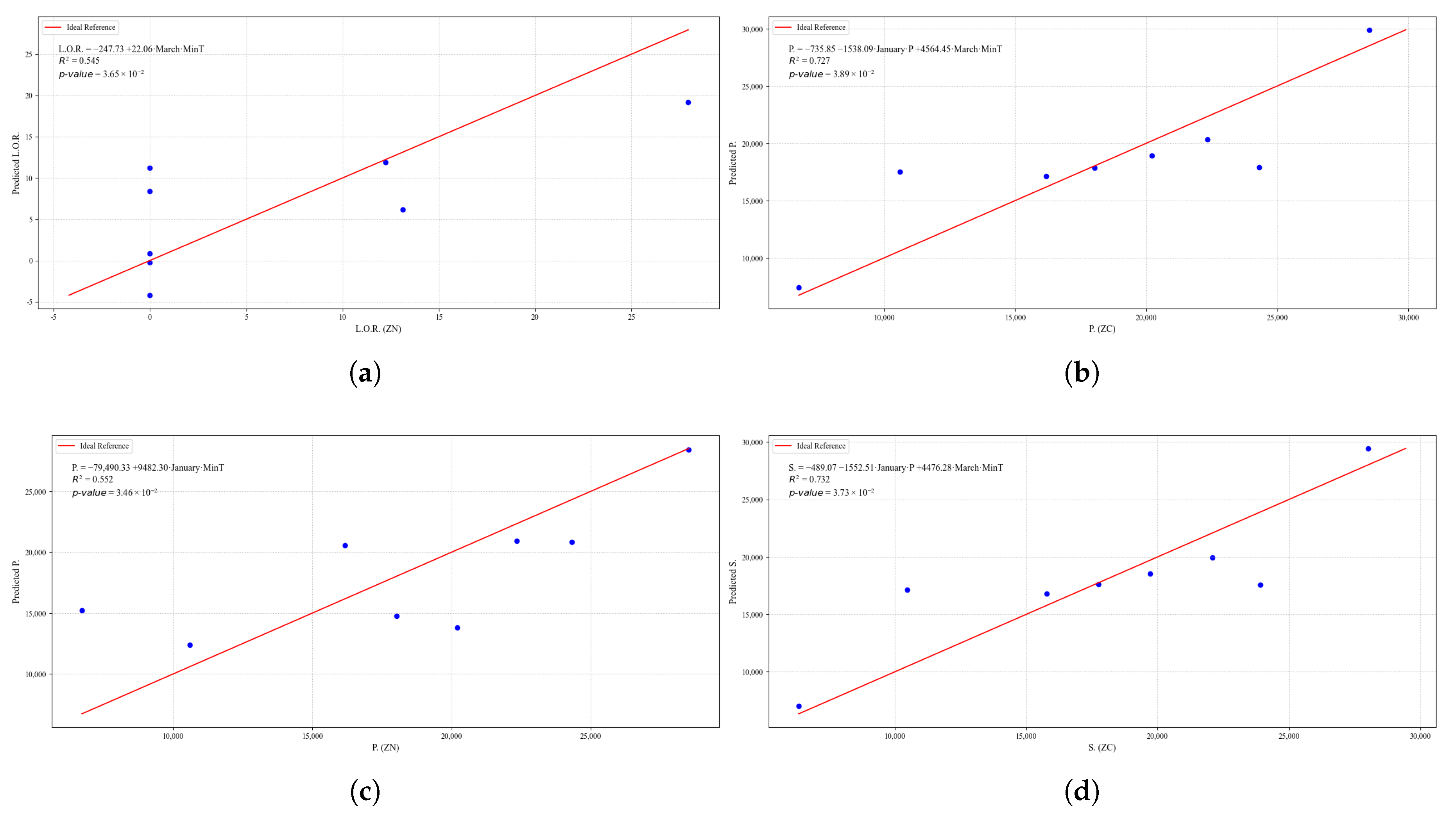
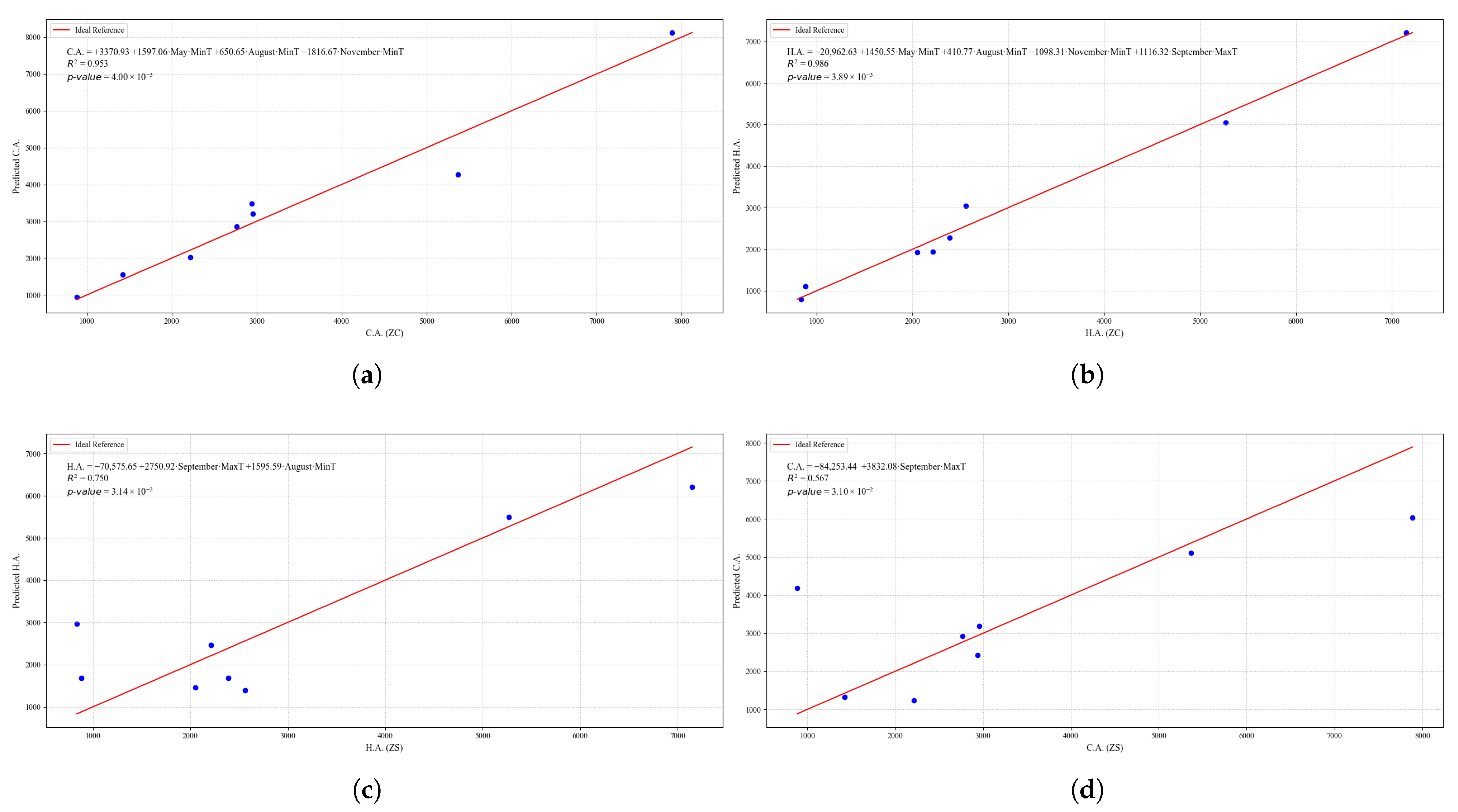
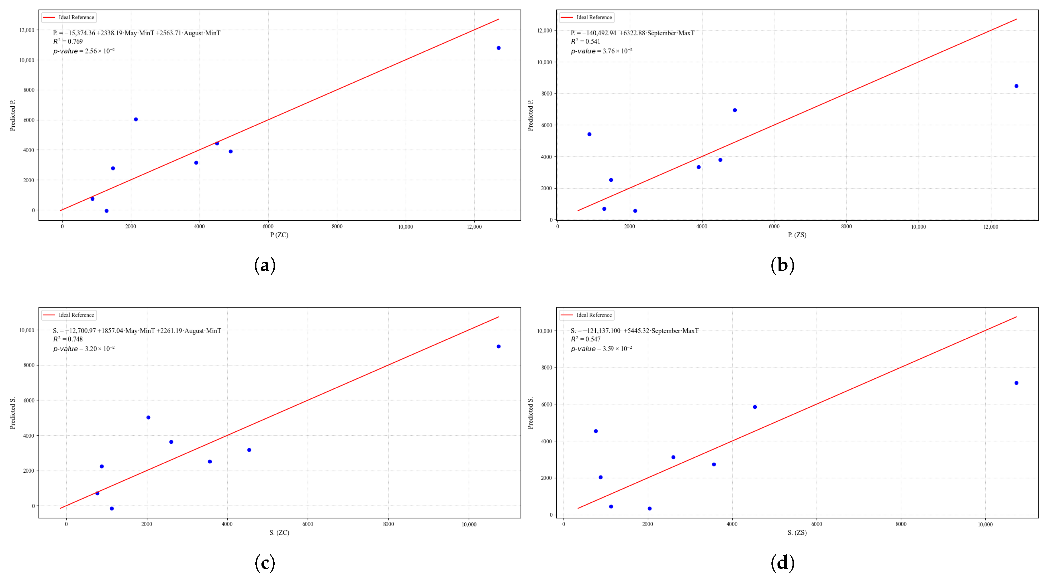
In the central zone, the cultivated area is associated with the minimum temperatures in May, August, and November, yielding an $R^2$ of 0.953, an adjusted $R^2$ of 0.946, and a p-value of 0.004. This indicates a highly fitted and statistically robust model, with low collinearity (VIF = 1.67) and a relatively small prediction error (LOYO MSE = $1.2\times {10}^6$). In contrast, in the southern zone, the maximum temperature in September explains the cultivated area with a more modest fit ($R^2$ = 0.567, $R_{adj}^2$ = 0.547, p = 0.031), but still within a statistically significant threshold. This contrast highlights the stronger role of minimum temperatures in the central zone compared to the greater influence of maximum temperatures in the southern zone.

Regarding the harvested area, the central zone shows exceptional explanatory power: the minimum temperatures in May, August, and November, combined with the maximum temperature in September, explain 98.6% of the variation ($R^2$ = 0.986, $R_{adj}^2$ = 0.984, p = 0.0039), with a low AICc and minimal error ($7.3\times {10}^5$). In the southern zone, the model including the minimum temperature in August and the maximum temperature in September also achieves statistical significance (p = 0.031), although the fit is more moderate ($R^2$ = 0.749). These results confirm that the central zone has more stable and less redundant predictors (VIF < 2), making the models there more reliable.

For production, in the central zone, the minimum temperatures in May and August explain 76.9% of the variability ($R_{adj}^2$ = 0.747, p = 0.025), evidencing statistical significance, though with higher predictive error compared to harvested area. In the southern zone, September maximum temperature remains the main explanatory variable, with a moderate yet significant fit ($R^2$ = 0.541, p = 0.0376).

For the sales variable, the central zone is influenced by the minimum temperatures in May and August, with $R_{adj}^2$ = 0.723 and p = 0.032, while in the southern zone, the maximum temperature in September contributes significantly ($R_{adj}^2$ = 0.527, p = 0.0359). This indicates that sales are moderately but consistently influenced by temperature extremes, particularly in months critical for plant development.

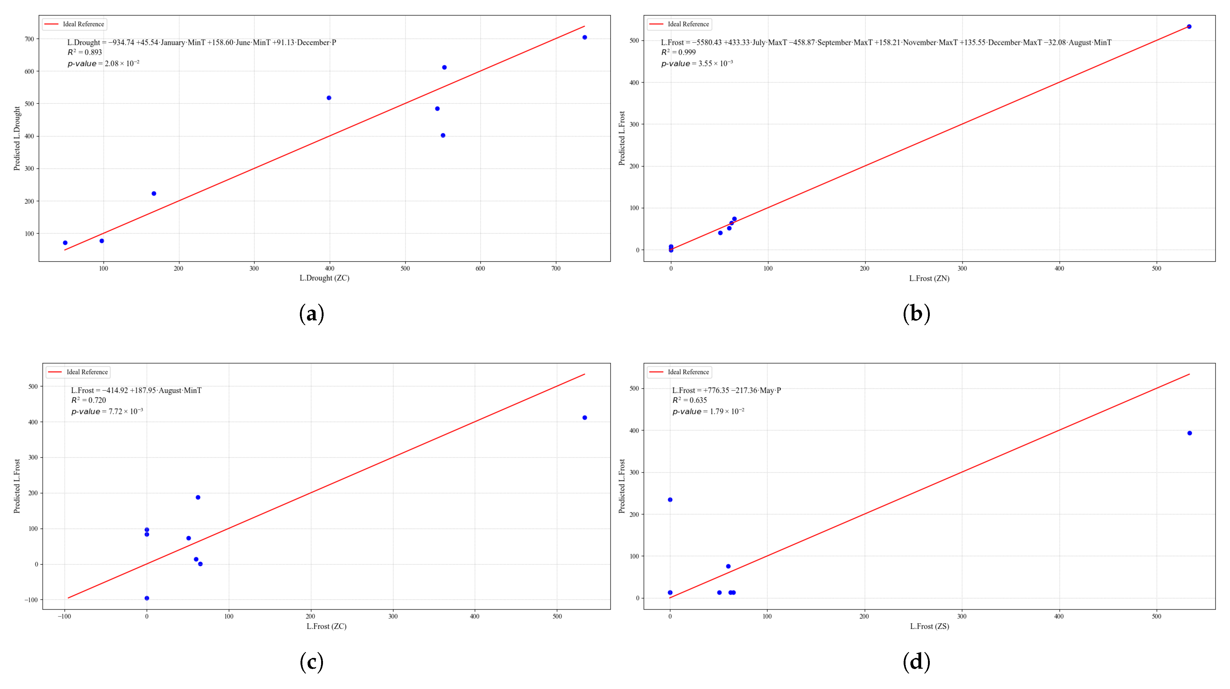
Regarding drought losses, the central zone presents a well-fitted model ($R^2$ = 0.892, $R_{adj}^2$ = 0.877, p = 0.0208), where January and June minimum temperatures and December precipitation are the main drivers, with low prediction error ($1.9\times {10}^4$). Conversely, the northern zone’s drought model is weak ($R_{adj}^2$ = 0.479, p = 0.917), suggesting that drought in this zone cannot be adequately captured with the current predictors.

Frost losses show significant associations in all three zones. In the northern zone, July to December temperatures generate a nearly perfect model ($R^2$ = 0.998, $R_{adj}^2$ = 0.998, p = 0.00355), although high multicollinearity (VIF = 27.21) questions the stability of the coefficients. In the central zone, August minimum temperature explains 72% of the variation ($R_{adj}^2$ = 0.707, p = 0.0077), whereas in the southern zone, May precipitation contributes significantly ($R_{adj}^2$ = 0.618, p = 0.0179).

For pest losses, the central zone stands out, as January, April, and June precipitation explain 96.8% of the variation ($R_{adj}^2$ = 0.964, p = 0.0018), with moderate collinearity (VIF = 8.47). In contrast, in the northern zone, the model explains only 54.2% of the variation and lacks statistical significance (p = 0.142), reflecting limited climatic predictability of pest dynamics there.

Disease losses in the central zone reach $R^2=1.0$ with $p=0$, which suggests overfitting, making the model less reliable for prediction. More realistic but still strong fits are observed in the southern zone ($R_{adj}^2$ = 0.960, p = 0.316), whereas the northern zone shows weak associations (p = 0.907).

Finally, in the northern zone, losses due to other causes are linked to April minimum temperature, with a moderate fit ($R_{adj}^2$ = 0.482, p = 0.048). In the southern zone, however, the model is statistically non-significant ($R_{adj}^2$ < 0, p = 0.896), confirming that these losses are not explained by climate alone.

Model Complexity, Overfitting

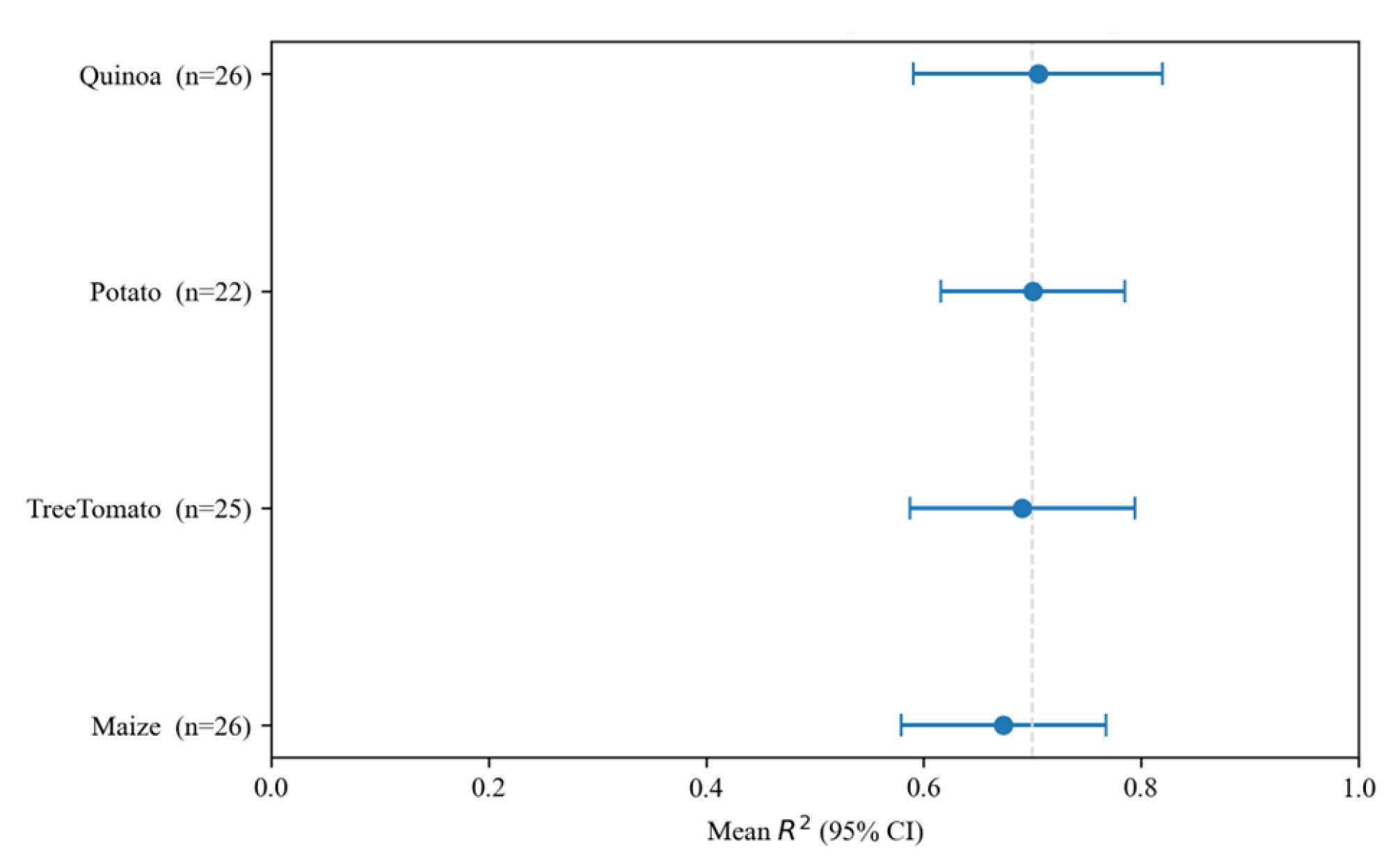
Our multiple linear regression results highlight the strong influence of climate variability on crop yields in the study areas. The average coefficient of determination ($R^2$) for the models is notably high (around 0.67–0.71 for the different crops), meaning roughly two-thirds of the interannual yield variation is explained by the selected climate extreme indices. This indicates that year-to-year weather anomalies (such as extreme temperatures and rainfall patterns) are closely tied to how much these crops produce each season. In fact, this level of explained variability is higher than the global average contribution of climate to yield variability (approximately one-third) reported in broad-scale studies [39]. Our regional focus likely captures a more pronounced climate signal, consistent with the idea that in certain areas (particularly rain-fed and climatically sensitive regions), over 60% of yield variability can be driven by climate fluctuations. Such high $R^2$ values suggest that the crops—including corn, potato, tree tomato, and quinoa—are highly sensitive to climate extremes in these zones. This aligns with previous research showing that temperature and precipitation extremes have significant impacts on crop growth and yield. For instance, extremely hot days can shorten the growing period and reduce grain filling, while droughts induce water stress, and intense rainfall can lead to flooding or waterlogged soils [40]. The implication is that variations in indices like heat-wave frequency or heavy rainfall days translate into tangible ups and downs in annual harvests.

Moreover, our analysis of the climate extreme indices over the study period confirms ongoing climatic changes in the region. We observe clear upward trends in temperature-related extremes: for example, the frequency of warm days and nights has increased in all zones, with a corresponding decrease in cold extremes, indicating a general warming trend. This is in agreement with wider South American climate observations that report a consistent rise in heat extremes (more frequent hot days/nights and fewer cold nights) over the past few decades [42]. In the case of precipitation, some zones exhibit a tendency toward more intense rainfall events—such as an increase in days with heavy rainfall—even if total annual rainfall remains variable. This pattern of fewer but more intense rain events, noted in our results, has also been documented at the continental scale. Such changes are critical because they can exacerbate agricultural risks: more intense downpours can damage crops and soil, while longer dry spells between rains increase drought stress. Overall, the concurrence of our findings with established climate extreme trends lends credibility to our results. It underscores that the study region is already experiencing the types of climate shifts (warming and rainfall intensity changes) that pose challenges to agriculture. Our regression results, combined with these observed climate trends, stress that without adaptation measures, the increasing occurrence of extreme weather events could significantly impact crop productivity and stability in the future. The strong climate–yield link identified here serves as a warning: as extremes continue to intensify under climate change, crop yields in these zones may become more volatile and vulnerable.

The figures depicting cultivated area (CA) and harvested area (HA) in the Central (ZC) and Southern (ZS) zones (Figure 22 and Figure 23 ) suggest that agricultural success in these regions is strongly linked to climatic conditions. These plots likely demonstrate that the amount of land farmers decide to sow and ultimately harvest is contingent upon temperatures and precipitation during critical months. The correlations identified in these figures are fundamental to understanding how climatic patterns influence large-scale crop management decisions and production outcomes.

Furthermore, the images representing losses due to various factors (Figure 24 and Figure 25) offer a crucial perspective on the risks farmers face. The figures on drought and frost losses (LDrought, LFrost) are pivotal, as they pinpoint the primary climatic drivers of crop failure. Additionally, the correlation between climate and pest losses (LPestsZC) highlights the link between environmental conditions and the incidence of biological outbreaks. Collectively, these plots illustrate how climatic variability not only affects potential yield but also introduces significant risks that can completely compromise production, thereby underscoring the necessity of zone-specific adaptation strategies.

The multiple regression models for corn (

Table A6. Summary of multiple linear regression models for different dependent variables of corn cultivation. The equations (month: predictors) are listed, along with $R^2$ and p-values.

Variable	Equations	${\mathit{R}}^2$	p-Value	${\mathit{R}}_{\mathbf{adj}}^2$	AICc	LOYO MSE	VIFmax
C.A.	July: MaxTempZN; December: MaxTempZN	0.715	0.0433	0.688	177.79	$5.4\times {10}^8$	2.41
	—	—	—	—	—	—	—
	—	—	—	—	—	—	—
H.A.	July: MaxTempZN; December: MaxTempZN	0.683	0.0565	0.653	175.37	$2.9\times {10}^8$	2.4
	—	—	—	—	—	—	—
	—	—	—	—	—	—	—
P.	July: PrecipitationZN; October: MinTempZN	0.665	0.0647	178.77	$3.5\times {10}^8$	2.09
	February: MinTempZC; June: MaxTempZC; September: PrecipitationZC; November: PrecipitationZC	0.914	0.0593	0.896	173.99	$8.0\times {10}^8$	17.11
	May: MinTempZS; September: PrecipitationZS	0.772	0.0246	0.751	175.68	$1.6\times {10}^8$	1.46
S.	—	—	—	—	—	—	—
	February: MinTempZC; March: PrecipitationZC; June: MaxTempZC; September: PrecipitationZC; November: PrecipitationZC	0.953	0.113	0.940	169.87	$3.97\times {10}^8$	17.26
	May: MinTempZS; June: MaxTempZS; September: PrecipitationZS	0.816	0.0591	0.789	173.97	$1.4\times {10}^8$	2.97
T.L.	July: MaxTempZN; December: MaxTempZN	0.619	0.0890	0.584	155.98	$5.9\times {10}^7$	2.4
	January: MinTempZC; December: MinTempZC	0.714	0.0436	0.687	153.7	$1.8\times {10}^7$	1.44
	—	—	—	—	—	—	—
L.Drought	June: PrecipitationZN; July: MaxTempZN, MinTempZN; August: MinTempZN; September: MaxTempZN; October: PrecipitationZN; November: MaxTempZN; December: MaxTempZN	1	0	0	0	0	0
	January: MinTempZC; May: MinTempZC; December: MinTempZC	0.892	0.0211	0.876	140.94	$3.8\times {10}^6$	1.76
	December: PrecipitationZS	0.509	0.0467	0.487	147.51	$5.6\times {10}^6$	1
L.Frost	March: PrecipitationZN; June: PrecipitationZN; August: PrecipitationZN; September: PrecipitationZN	0.92008	0.0538	0.903	117.91	$2.3\times {10}^5$	78.01
	April: PrecipitationZC	0.612	0.0216	0.595	121.77	$3.9\times {10}^5$	1
	March: PrecipitationZS; April: MaxTempZS; July: PrecipitationZS	0.807	0.0651	0.778	121.72	$2.7\times {10}^5$	2.15
L.Pests	May: PrecipitationZN; July: MaxTempZN	0.644	0.0756	0.610	126.47	$3.9\times {10}^5$	2.45
	June: MinTempZC	0.588	0.0263	0.57	125	$3.3\times {10}^5$	1
	June: PrecipitationZS	0.699	0.00970	0.685	122.50	$2.6\times {10}^5$	1
L.Diseases	February: PrecipitationZN; March: MinTempZN; May: PrecipitationZN; July: MaxTempZN; August: MaxTempZN	0.948	0.123	0.934	90.70	$6.7\times {10}^4$	9.2
	June: MinTempZC	0.774	0.00391	0.765	90.15	$4.7\times {10}^3$	1
	June: PrecipitationZS; November: MinTempZS, PrecipitationZS	0.745	0.110	0.708	96.66	$1.2\times {10}^4$	2.73
L.Flooding	March: MaxTempZN, PrecipitationZN; May: MinTempZN; June: MaxTempZN, PrecipitationZN; July: PrecipitationZN; September: MaxTempZN; November: PrecipitationZN	1	0	0	0	0	0
	March: PrecipitationZC; May: MinTempZC; July: PrecipitationZC	0.905	0.0162	0.891	115.29	$3.4\times {10}^5$
	April: MaxTempZS; May: MinTempZS	0.709	0.0454	0.682	121.37	$2.8\times {10}^5$	1.95
L.O.R.	July: MaxTempZN; August: MinTempZN; December: MaxTempZN	0.819	0.0573	0.792	134.34	$5.02\times {10}^6$	11.66
	—	—	—	—	—	—	—
	May: PrecipitationZS	0.583	0.0273 0.565	135.49	$3.4\times {10}^6$	1

and Figure A42, Figure A43, Figure A44) show variable explanatory power across zones and dependent variables. In the northern zone, cultivated and harvested area are moderately explained by maximum temperatures in July and December ($R^2\approx$ 0.65–0.69, $p<0.05$). Production and sales exhibit higher fits in the central and southern zones ($R_{adj}^2$ between 0.75 and 0.91), although with differences in statistical robustness.

For abiotic constraints, drought and flooding losses present the strongest models in the central zone ($R_{adj}^2$ > 0.87, $p<0.05$), while frost losses are better explained in the northern zone ($R_{adj}^2$ = 0.90) despite high collinearity. Pest and disease losses reach significant fits mainly in the central and southern zones ($R_{adj}^2$ = 0.57–0.77). Finally, losses due to other reasons show moderate but significant explanatory power in the northern and southern zones ($R_{adj}^2\approx$ 0.56–0.79, $p<0.06$).

The multiple regression models for potato (

Table A7. Summary of multiple linear regression models for different dependent variables of potato cultivation. The equations (month: predictors) are listed, along with $R^2$ and p-values.

Variable	Equations	${\mathit{R}}^2$	p-Value	${\mathit{R}}_{\mathbf{adj}}^2$	AICc	LOYO MSE	VIFmax
C.A.	February: MaxTempZN, PrecipitationZN	0.6809	0.0575	0.651	157.89	$3.23\times {10}^7$	3.75
	—	—	—	—	—	—	—
	January: MinTempZS; March: MinTempZS; August: PrecipitationZS	0.735	0.119	0.696	159.28	$2.2\times {10}^7$	8.24
H.A.	February: MaxTempZN, PrecipitationZN; October: MaxTempZN	0.736	0.118	0.697	157.73	$2.5\times {10}^7$	4.64
	—	—	—	—	—	—	—
	January: MinTempZS; March: MinTempZS; August: PrecipitationZS	0.733	0.121	0.693	157.62	$2.1\times {10}^7$	8.24
P.	February: MaxTempZN, PrecipitationZN; April: MaxTempZN; October: MaxTempZN	0.958	0.0206	0.95	189.54	$2.2\times {10}^9$	5.91
	—	—	—	—	—	—	—
	January: MinTempZS; March: MinTempZS; November: MaxTempZS	0.770	0.0911	0.736	200.03	$9.0\times {10}^9$	10.80
S.	February: MaxTempZN, PrecipitationZN; October: MaxTempZN	0.887	0.0226	0.871	192.21	$1.5\times {10}^9$	4.64
	January: MaxTempZC; October: PrecipitationZC	0.719	0.0418	0.692	196.66	$1.9\times {10}^9$	1.25
	January: MinTempZS; March: MinTempZS; November: MaxTempZS	0.792	0.0748	0.762	197.13	$6.8\times {10}^9$	10.8
T.L.	October: MaxTempZN	0.736	0.00639	0.725	89.81	$4.3\times {10}^3$	1
	March: PrecipitationZC; July: PrecipitationZC; August: PrecipitationZC; February: MaxTempZC; March: MaxTempZC; May: MinTempZC	0.927	0.483	0.901	95.98	$8.3\times {10}^5$	16.25
	February: MinTempZS; August: MinTempZS, PrecipitationZS	0.728	0.125	0.687	95.60	$2.6\times {10}^4$	4.6
L.Drought	—	—	—	—	—	—	—
	—	—	—	—	—	—	—
	June: MaxTempZS, PrecipitationZS	0.712	0.0443	0.685	125	$3.9\times {10}^5$	2.31
L.Frost	—	—	—	—	—	—	—
	December: MinTempZC	0.504	0.0483	0.482	116.13	$9.1\times {10}^4$	1
	—	—	—	—	—	—	—
L.Pests	January: PrecipitationZN; June: PrecipitationZN; September: MaxTempZN; November: MaxTempZN	0.759	0.252	0.709	113.22	$8.3\times {10}^5$	9.44
	September: PrecipitationZC	0.581	0.0277	0.563	108.89	$4.4\times {10}^4$	1
	—	—	—	—	—	—	—
L.Diseases	January: MaxTempZN, MinTempZN; February: MaxTempZN; May: MaxTempZN, MinTempZN	0.816	0.397	0.765	119.7	$1.5\times {10}^6$	54.06
	March: MinTempZC; October: MinTempZC	0.669	0.0630	0.637	114.68	$3.3\times {10}^5$	1.63
	January: MinTempZS; March: MaxTempZS, MinTempZS; November: MinTempZS	0.876	0.101	0.85	112.95	$16.85\times {10}^4$	$1.5\times {10}^5$
							16.85
L.Flooding	January: MinTempZN; June: PrecipitationZN	0.880	0.00499	0.869	81.17	$2.3\times {10}^3$	2.14
	—	—	—	—	—	—	—
	—	—	—	—	—	—	—
L.O.R.	January: MaxTempZN; March: MaxTempZN, PrecipitationZN; May: MaxTempZN, MinTempZN; June: MaxTempZN; July: MaxTempZN; August: MaxTempZN; September: MaxTempZN, MinTempZN; November: PrecipitationZN	1	0	0	0	0	0
	—	—	—	—	—	—	—
	March: MaxTempZS; April: MaxTempZS; May: MaxTempZS	0.816	0.0588	0.79	85.15	$2.1\times {10}^3$	7.94

) show variable explanatory power across zones and dependent variables. For cultivated and harvested area (C.A., H.A.), the northern zone is moderately explained by maximum temperature and precipitation in February (adjusted $R^2\approx 0.65$; $p=0.058$). In the southern zone, combinations of minimum and precipitation variables in January, March, and August provide moderate fits ($R_{adj}^2\approx 0.69$–0.70; $p=0.12$).

Production (P.) exhibits strong explanatory power in the northern zone with February and October temperatures and precipitation ($R_{adj}^2=0.95$, $p=0.021$). In the southern zone, January–March variables yield moderate fits ($R_{adj}^2\approx 0.74$; $p=0.09$). Sales (S.) show a similar pattern, with high fits in the northern zone ($R_{adj}^2=0.87$; $p=0.023$) and moderate fits in central and southern zones ($R_{adj}^2\approx 0.69$–0.76; $p=0.04$–0.075).

Technical losses (T.L.) are explained by October temperatures in ZN ($R_{adj}^2=0.725$, $p=0.006$) and combinations of precipitation and temperature in ZC and ZS with moderate adjusted $R^2$ (0.687–0.901). Drought losses (L.Drought) are only significant in the southern zone ($R_{adj}^2=0.685$, $p=0.044$). Frost losses (L.Frost) show marginal significance in the central zone ($R_{adj}^2=0.482$, $p=0.048$).

For pest losses (L.Pests), central and southern zones reach modest explanatory power ($R_{adj}^2\approx 0.56$–0.71), with significance only for the ZC model ($p=0.028$). Disease losses (L.Diseases) present moderate to strong fits in all zones ($R_{adj}^2\approx$ 0.637–0.85), though significance is borderline in most cases. Flooding losses (L.Flooding) are explained in the northern zone by January and June variables ($R_{adj}^2=0.869$, $p=0.005$). Finally, losses due to other reasons (L.O.R.) reach perfect fit in ZN ($R^2=1$, $p=0$) and moderate fit in ZS ($R_{adj}^2=0.79$, $p=0.059$), reflecting substantial climate influence in the northern zone and moderate influence in the southern zone.

The regression models for tree tomato (

Table A9. Summary of multiple linear regression models for different dependent variables of tree tomato cultivation. The equations (month: predictors) are listed, along with $R^2$ and p-values.

Variable	Equations	${\mathit{R}}^2$	p-Value	${\mathit{R}}_{\mathbf{adj}}^2$	AICc	LOYO MSE	VIFmax
L.Flooding	January: MinTempZN; March: MinTempZN; April: MaxTempZN	0.867	0.0316	0.847	78.39	$1.1\times {10}^3$	2.94
	March: MinTempZC	0.792	0.00305	0.783	76.42	1136.3	1
	January: MinTempZS; March: MinTempZS	0.593	0.105	0.55	84.42	2984.29	6.85
L.O.R.	March: MinTempZN	0.544	0.0365	0.524	57.28	89.41	1
	February: MinTempZC; June: MaxTempZC; September: PrecipitationZC; October: MinTempZC; November: PrecipitationZC	0.963	0.0891	0.953	49.49	187.02	20.53
	April: PrecipitationZS; September: PrecipitationZS; November: MinTempZS	0.692	0.0524	0.646	57.67	92.12	—

) show variable explanatory power depending on the dependent variable and zone. Production and sales are moderately explained in the northern zone by January minimum temperatures ($R_{adj}^2\approx 0.53$–0.53; $p\approx 0.035$). In the central zone, January precipitation combined with March minimum temperatures improves the fit ($R_{adj}^2\approx 0.70$; $p\approx 0.038$).

Technical losses (T.L.) show high explanatory power across zones, particularly in ZS with perfect fit ($R^2=1$, $p=0$). Drought and frost losses are explained moderately by temperature and precipitation variables in all zones ($R_{adj}^2\approx 0.73$–0.81), with some high collinearity in ZN and ZS.

Pest and disease losses exhibit strong fits in the central and southern zones ($R_{adj}^2\approx 0.95$–0.97; $p<0.01$), while northern zone models are moderate ($R_{adj}^2\approx 0.49$–0.73). Flooding losses reach high fits in the northern and central zones ($R_{adj}^2=0.78$–0.85; $p<0.032$).

Finally, losses due to other reasons (L.O.R.) show moderate fits in the northern and southern zones ($R_{adj}^2\approx 0.52$–0.65) and high fit in the central zone ($R_{adj}^2=0.953$), highlighting the combined influence of temperature and precipitation on yield reduction.

5.3. Cross-Crop Synthesis of Climate Effects

To compare patterns across crops and zones, we added two complementary summaries: (i) a heatmap of model fit ($R^2$) by crop–zone and outcome, and (ii) a forest plot which synthesizes, for each crop, the mean $R^2$ with 95% confidence intervals across all valid models (giving priority to $R_{\mathrm{adj}}^2$ when available). Each crop–zone–outcome cell in the heatmap corresponds to the best-performing specification retained after our screening steps, while blank cells indicate that no stable model passed the selection criteria. Figure 26 and Figure 27 summarize these results.

The heatmap (Figure 26) reveals where and for which outcomes the climate signal is strongest. Quinoa presents consistently high fits across outcomes, particularly in ZC. corn achieves moderate to high fits in ZC and the ZS, with precipitation featuring prominently in loss models. Potato shows its strongest performance in ZN—notably for production and sales—while ZS retains useful but comparatively weaker signal. Tree tomato exhibits a moderate signal: ZN is largely explained by minimum temperature for production/sales, whereas ZC combines precipitation and minimum temperature. The forest plot (Figure 27) condenses these patterns: quinoa attains the highest mean $R^2$ with relatively tight uncertainty; potato follows with solid mean performance; corn is moderate; and tree tomato, while lower on average, still displays meaningful predictability in specific zone–outcome combinations. The confidence-interval widths reflect heterogeneity across outcomes and zones.

The comparative patterns in Figure 26 and Figure 27 agree with the crop-specific tables reported in the Results section: (i) for quinoa, high $R^2$ values are recurrent for production and sales, with MinTemp dominating ZC and MaxTemp recurring in ZN (July–December); (ii) for corn, precipitation repeatedly enters loss models (flooding/frost) and several production/sales models in ZC/ZS; (iii) for potato, ZN models for production and sales present the highest fits, driven by MaxTemp and episodic precipitation; (iv) for tree tomato, ZN production/sales rely on MinTemp, while ZC mixes Precipitation and MinTemp. Where variance inflation factors (VIF) are large in some loss models, we emphasize the recurrence and direction of predictors rather than coefficient magnitudes.

Key Findings by Crop

• Quinoa. (1) Consistently strong fits across outcomes, especially in ZC; (2) ZN models frequently involve MaxTemp in the late dry season (Jul–Dec), whereas ZC is largely driven by MinTemp (May–Nov); (3) Several loss categories attain high $R^2$, but some present elevated VIF, so interpretation focuses on stable predictor patterns.
• Corn. (1) Moderate–high skill in ZC and ZS for production/sales, with precipitation recurring from March to November; (2) Loss models for flooding/frost are precipitation-sensitive (hydrometeorological control); (3) MinTemp in late boreal winter and MaxTemp near the growing season contribute in ZC/ZS, while ZN shows weaker signal.
• Potato. (1) Best performance in ZN for production and sales (dominant role of MaxTemp plus episodic precipitation); (2) Losses by flooding are well explained in ZN, while drought losses show better skill in ZS, evidencing north–south vulnerability contrasts; (3) ZS retains useful signal for production/sales, albeit weaker than ZN.
• Tree tomato. (1) Moderate predictability: ZN production/sales explained largely by MinTemp; (2) ZC combines Precipitation and MinTemp with acceptable fits; (3) Several loss models achieve high $R^2$ values, but with multicollinearity in some cases (high VIF), so inference prioritizes predictor recurrence.

Together, the heatmap and forest plot demonstrate that climate drivers are crop- and zone-specific rather than uniform across the Ecuadorian highlands. Temperature extremes drive quinoa (ZN) and potato (ZN), while minimum temperature and precipitation combinations are crucial for quinoa/tree tomato (ZC) and for corn losses across ZC/ZS. These cross-crop syntheses complement the detailed model tables and support the main narrative: climate variability exerts differentiated pressures along the N–C–S gradient and across crops. Given occasional multicollinearity in some loss models, we constrain interpretation to consistent signals across months and zones, using $R_{\mathrm{adj}}^2$ when available and cross-validatory diagnostics as reported. Overall, the comparative lens reinforces the robustness of the crop-specific findings and clarifies where climate management and risk-reduction efforts (e.g., frost and flooding preparedness) may yield the largest benefits.

5.4. Extreme-Event Diagnostics (2015–2022)

To complement the monthly climate summaries used in the regression analysis, we characterized the intra-seasonal occurrence of extremes for each highland zone using daily NASA POWER (MERRA-2) fields at 0.5° resolution over 2015–2022. For each zone (North, Center, South), we sampled three interior locations (centroid plus two interior points), computed point-level indices, and aggregated annual medians by zone. We considered four simple, ETCCDI-style indicators: (i) Frost days (days with $T_{min}<0^{\circ }$C), (ii) Heat days (days with $T_{max}$ above the point-specific 90th percentile; TX90), (iii) Dry spells (number of runs ≥5 consecutive days with $p=0$), and (iv) CDD_max (maximum number of consecutive dry days per year). Linear trends were estimated for 2015–2022 at the zone scale to provide context for recent variability.

5.4.1. Frost Days

Across the three zones, the reanalysis yields virtually zero frost days throughout the period (Figure 28). Given the complex topography of the Ecuadorian highlands and the coarse spatial resolution, this outcome is consistent with under-detection of localized valley and páramo frosts. In the remainder of this paper, frost risk is thus interpreted primarily from monthly statistics and reported loss records rather than from daily POWER thresholds.

5.4.2. Heat Days (TX90)

The annual number of heat days displays interannual variability in all zones, with a tendency toward lower counts toward the end of the record (Figure 29). These tendencies are weak and not statistically compelling at this temporal scale, but they indicate no recent intensification of short-duration heat stress at the zone level.

5.4.3. Dry Spells and CDD_max

Signals of intra-season dryness are most pronounced in the South (Cañar–Azuay–Loja). This zone concentrates the largest number of ≥5-day dry spells and exhibits the longest annual dry sequences (CDD_max, up to ∼8 days), with modest upward tendencies over 2015–2022 (Figure 28, Figure 29, Figure 30 and Figure 31). The center shows smaller, non-significant increases, while the north remains comparatively low and flat. These patterns are consistent with the regression results where precipitation-related predictors are more influential in the southern highlands.

5.4.4. Interpretation Within the Study Framework

Taken together, the daily diagnostics provide a process-oriented backdrop to the monthly covariates used in the models. The lack of reanalysis-detected frost events cautions against using gridded Tmin alone to represent local frost exposure, whereas the concentration of dry-spell metrics in the south agrees with the stronger sensitivity of agricultural outcomes to precipitation found in that region. The short (eight-year) window and the coarse grid resolution limit trend detection; therefore, these indices are interpreted as recent context rather than long-term change.

6. Conclusions

Although the results have been extensively discussed in previous sections, this section presents conclusions that integrate all points of analysis.

One of the main findings from the analysis of the four products in the production segment and their relationship with climatic factors (maximum temperature, minimum temperature, and precipitation) is the increasing frequency and intensity of adverse climatic events. These events cause substantial damage, becoming one of the most critical challenges in the management of high-Andean food systems.

Another critical issue is the lack of technological tools to provide early warnings of potential adverse climatic events, enabling farmers to take appropriate measures in production and avoid losses. Changes in climatic patterns have also altered the incidence of pests and diseases, causing significant damage to crops and consequently reducing farmers’ incomes. A clear example is the so-called “Punta Morada”, which affects solanaceous crops in general.

Regarding performance indicators, Ecuador has not yet achieved productive efficiency in the four crops analyzed. When comparing production against consumption, the balance remains negative, meaning that domestic demand is not fully met. National prices are lower than international ones, and the distribution of profits along the value chain is inequitable: the price received by producers is lower than that obtained by wholesale traders, even though the greatest investment and risk are borne by farmers in the production stage. Yield trends for each crop have been fluctuating, reaching a peak in 2019, decreasing in 2020, and then increasing again in 2021 and 2022.

The share of corn, potato, quinoa, and tree tomato in Ecuador’s non-oil exports does not exceed 1%. Regarding multiplier effects, the number of companies involved in supplying agricultural inputs has fluctuated, reaching its peak in 2021 before declining again in 2022.

According to the analysis of climatic variables and agricultural production variables of high-Andean products, several noteworthy results emerge. For corn cultivation in the central zone, the analyses indicate a significant impact of precipitation on frost losses, as well as the combined influence of the three climatic factors (maximum temperature, minimum temperature, and precipitation) on disease-related losses. In the southern zone, climatic variables have a considerable impact on losses attributed to other causes. Climate emerges as a major—but not exclusive—driver of yield variability.

For potato cultivation, total sales in the northern zone show a moderate relationship with maximum temperature in October. In the southern zone, sales exhibit a similar but less significant relationship. This suggests that, in certain regions, maximum temperature in October can serve as a good indicator of total sales. Frost losses in the central zone present a moderate relationship with minimum temperature in December, indicating that this variable is a good predictor of frost-related losses in that region. Pest losses in the central zone display a strong association with precipitation in January, June, and September, suggesting that precipitation is a reliable predictor of pest-related losses in this area. Flood losses in the northern zone show a strong relationship with minimum temperatures in January and precipitation in June, implying that the selected climatic variables are good predictors of flood-related losses. Losses due to other causes exhibit a moderate and significant relationship with maximum and minimum temperatures.

Regarding quinoa cultivation, in the southern zone, maximum temperatures in September exhibit a moderate and significant relationship with the cultivated area. In the central zone, minimum temperatures in May, August, September, and November explain 98.6% of the variability in harvested area. In the southern zone, there is a moderate and significant relationship between temperatures in August and September and the harvested area. In the central zone, production and minimum temperatures in May and August explain 76.9% of the variability. Conversely, in the southern zone, maximum temperature in September shows a moderate and significant relationship with production. In the central zone, minimum temperatures in January and June, along with precipitation in December, explain 89.2% of the variability, with this relationship being statistically significant. Frost losses in the northern zone have an extremely strong relationship with maximum and minimum temperatures in July, August, September, November, and December. In the southern zone, precipitation in May has a moderate and significant relationship with frost losses. In the central zone, precipitation in January, April, and June exhibits a very strong relationship with pest losses.

For the tamarillo (Solanum betaceum) crop, in the northern zone, production shows a moderate relationship with the minimum temperature in January. In the central zone, the minimum temperature in March is a good predictor of frost losses. In the southern zone, minimum temperatures in January, March, and September, together with precipitation, explain 95.5% of the variability. In the northern zone, flood losses show a strong relationship with minimum temperatures in January and March and maximum temperature in April. In the central zone, the relationship is weaker.

The analysis of the effects of climatic factors—maximum and minimum temperatures and precipitation—on corn, potato, quinoa, and tamarillo in Ecuador’s high-Andean regions shows that adverse climatic events increasingly affect production, harvested area, sales, and losses, with distinct regional patterns. Central-zone crops are particularly sensitive to frost, pests, and precipitation variability, suggesting the need for frost-resistant varieties, pest monitoring, and adaptive planting schedules. Southern-zone crops are more impacted by high temperatures and drought, indicating the importance of heat- and drought-tolerant varieties, supplemental irrigation, and water management strategies. Northern-zone crops are mainly affected by floods and frost, highlighting the value of flood mitigation, drainage infrastructure, and early warning systems. These findings demonstrate that climate is a major, though not exclusive, driver of agricultural variability, and they underscore the necessity of integrating region-specific climate adaptation measures with technological, infrastructural, and policy support to enhance productivity, resilience, and sustainability in Ecuador’s high-Andean food systems.

Compared with traditional field monitoring (on-farm plots and local weather stations), the combination of NASA reanalysis datasets and ESPAC agricultural statistics offers clear advantages in terms of spatial and temporal coverage, as it allows for multi-year analyses over large areas at very low cost and with high reproducibility, since the datasets are openly accessible and consistently updated. However, limitations include potential biases in satellite/reanalysis estimates, the monthly resolution of the climate series, and the aggregation of official statistics that may mask local variability. Thus, while our approach provides a scalable baseline for regional risk assessment, it should be seen as complementary to fine-scale field monitoring, experimental plots, and local weather stations, which remain essential for calibration and for capturing microclimatic and management effects.

Building on the comparative crop–zone analysis, we outline concrete, region-specific measures that align with observed sensitivities:

North (ZN). Where warm-season Tmax exerts a strong influence and frost losses are reported, prioritize: (i) active frost protection at critical phenophases (e.g., overhead/sprinkler systems or air-mixing devices during radiation frost nights) [43,44]; (ii) sowing-date adjustments to avoid flowering/grain filling during peak frost windows; and (iii) tactical deficit irrigation where water is limiting, concentrating applications on drought-sensitive stages for quinoa and potato [45,46].

Center (ZC). With precipitation-driven risks (flooding, pests) peaking in late boreal winter to early boreal summer, strengthen drainage and runoff management (contour channels, terrace maintenance), deploy pest early warnings tied to wet-month thresholds, and use protective mulches/cover crops to buffer soil moisture and reduce splash-mediated disease spread [47].

South (ZS). Under stronger dry-spell/heat-day signals, expand water harvesting (cisterns, small reservoirs), regulated deficit irrigation focused on flowering and early filling [45], windbreaks/shade elements for tree tomato, and cold-air management (site selection away from frost pools). Across regions, leveraging Andean terrace know-how and ecosystem-based practices enhances resilience at low cost [48,49].

These measures translate this paper’s quantitative patterns into actionable, zone-specific options consistent with established agronomic and agroecological evidence while remaining compatible with the dataset and methods used here.

Finally, regarding multiple linear regressions, the models show variability in their ability to explain agricultural variables, with several cases of overfitting or lack of statistical significance. Factors not considered, such as agricultural infrastructure and support policies, likely play an important role in agricultural variability beyond the climatic variables considered here. A more holistic approach that considers both climatic and non-climatic factors is necessary to better understand agricultural dynamics in the Ecuadorian context.

References

1. Saenz-Lituma, G. The agroecological transition of farms in the Ecuadorian highlands: New tools for monitoring and supporting agroecological transition. Land Degrad. Dev. 2025, 36, 424–440. [Google Scholar] [CrossRef]
2. Vallejo-Rojas, V.; Ravera, F.; Rivera-Ferre, M.G. Developing an integrated framework to assess agri-food systems and its application in the Ecuadorian Andes. Reg. Environ. Change 2016, 16, 2171–2185. [Google Scholar] [CrossRef]
3. Vallejo-Rojas, V.; Ravera, F.; Rivera-Ferre, M. The agri-food system (re)configuration: The case study of an agroecological network in Andean Ecuador. Agric. Hum. Values 2022, 39, 1301–1327. [Google Scholar] [CrossRef]
4. Francis, C.; Lieblein, G.; Gliessman, S.; Breland, T.A.; Creamer, N.; Harwood, R.; Salomonsson, L.; Helenius, J.; Rickerl, D.; Salvador, R.; et al. Agroecology: The Ecology of Food Systems. J. Sustain. Agric. 2003, 22, 99–118. [Google Scholar] [CrossRef]
5. Navarrete, I.; Parra-Rondinel, F.; Scurrah, M.; Bonifacio, A.; Andrade-Piedra, J.L. Recent developments for robust potato seed systems through agrobiodiversity and farmers engagement in the Andes. Curr. Opin. Environ. Sustain. 2024, 69, 101454. [Google Scholar] [CrossRef]
6. Altieri, M.A.; Koohafkan, P. Enduring Farms: Climate Change, Smallholders and Traditional Farming Communities; Third World Network: Penang, Malaysia, 2008. [Google Scholar]
7. Carrasco-Torrontegui, A. Climate Change, Food Sovereignty and Ancestral Farming Technologies in the Andes. Curr. Dev. Nutr. 2020. [Google Scholar] [CrossRef]
8. Gallegos-Riofrío, C.A.; Carrasco-Torrontegui, A.; Riofrio, L.A.; Waters, W.F.; Iannotti, L.L.; Pintag, M.; Caranqui, M.; Ludeña-Maruri, G.; Burneo, J.N.; Méndez, V.E. The agroecological landscape of Caliata as a cue for planetary health. Agroecol. Sustain. Food Syst. 2022, 46, 842–876. [Google Scholar] [CrossRef]
9. Food and Agriculture Organization of the United Nations (FAO). Andean Agriculture: Globally Important Agricultural Heritage Systems. FAO GIAHS Program Document. 2020. Available online: https://www.fao.org/giahs/en (accessed on 12 May 2025).
10. Koohafkan, P.; Altieri, M.A. Globally Important Agricultural Heritage Systems: A Legacy for the Future; Food and Agriculture Organization of the United Nations: Rome, Italy, 2011. [Google Scholar]
11. Koohafkan, P.; Cruz, M.J.D. Conservation and Adaptive Management of Globally Important Agricultural Heritage Systems (GIAHS). J. Resour. Ecol. 2011, 2, 22–28. [Google Scholar] [CrossRef]
12. Food and Agriculture Organization (FAO). Globally Important Agricultural Heritage Systems (GIAHS). Overview of GIAHS Program Recognizing Heritage Agricultural Systems Worldwide. 2023. Available online: https://www.fao.org/giahs/en/ (accessed on 10 July 2025).
13. Caviedes, J. Indigenous and local knowledge on social-ecological changes is associated with small-scale farmers’ livelihood resilience. Agric. Syst. 2024, 216, 103885. [Google Scholar] [CrossRef]
14. Bazile, D.; Pulvento, C.; Verniau, A.; Al-Nusairi, M.S.; Ba, D.; Breidy, J.; Hassan, L.; Mohammed, M.I.; Mambetov, O.; Otambekova, M.; et al. Worldwide Evaluations of Quinoa: Preliminary Results from Post International Year of Quinoa FAO Projects in Nine Countries. Front. Plant Sci. 2016, 7, 850. [Google Scholar] [CrossRef]
15. Jaikishun, S.; Li, W.; Yang, Z.; Song, S. Quinoa: In Perspective of Global Challenges. Agronomy 2019, 9, 176. [Google Scholar] [CrossRef]
16. Hannah, L.; Ikegami, M.; Hole, D.G.; Seo, C.; Butchart, S.H.M.; Peterson, A.T.; Brooks, T.M. Global Climate Change Adaptation Priorities for Biodiversity and Food Security. PLoS ONE 2013, 8, e72590. [Google Scholar] [CrossRef]
17. Rötter, R.P.; Tao, F.; Hohn, J. Climate change impacts on maize production potential in the 21st century: A global meta-analysis. Glob. Change Biol. 2021, 27, 2806–2824. [Google Scholar] [CrossRef]
18. Lipper, L.; Thornton, P.; Campbell, B.M.; Baedeker, T.; Braimoh, A.; Bwalya, M.; Caron, P.; Cattaneo, A.; Garrity, D.; Henry, K.; et al. Climate-smart agriculture for food security. Nat. Clim. Change 2014, 4, 1068–1072. [Google Scholar] [CrossRef]
19. Hinojosa, L.; Gonzalez, J.A.; Barrios-Masias, F.H.; Fuentes, F.; Murphy, K.M. Quinoa abiotic stress responses: A review. Plants 2018, 7, 106. [Google Scholar] [CrossRef] [PubMed]
20. Ain, Q.T.; Siddique, K.; Bawazeer, S.; Ali, I.; Mazhar, M.; Rasool, R.; Mubeen, B.; Ullah, F.; Unar, A.; Jafar, T.H. Adaptive mechanisms in quinoa for coping in stressful environments: An update. PeerJ 2023, 11, e14832. [Google Scholar] [CrossRef]
21. Lopez, G.; Gaiser, T.; Ewert, F.; Srivastava, A. Effects of Recent Climate Change on Maize Yield in Southwest Ecuador. Atmosphere 2021, 12, 299. [Google Scholar] [CrossRef]
22. Tang, L.; Zhang, H.; Li, X. Genetic diversity and nutritional quality of quinoa (Chenopodium quinoa Willd.) and its potential as a future crop for food security under climate change. Plant Sci. 2021, 304, 110828. [Google Scholar] [CrossRef]
23. Bazile, D.; Jacobsen, S.E.; Verniau, A.; Hinojosa, F.; Mujica, A. Quinoa value chains in Andean countries: Challenges and opportunities for sustainable development. J. Agrar. Change 2020, 20, 275–294. [Google Scholar] [CrossRef]
24. Ferreira, M.; Muñoz, C.; Ramírez, S.; Smith, J. Seed systems and genetic diversity of quinoa in traditional Andean communities. Genet. Resour. Crop Evol. 2022, 69, 917–932. [Google Scholar] [CrossRef]
25. Valle, M.; González, P.; Fernandez, E. Cultural heritage and agroecological resilience: Farmers’ knowledge on quinoa in the high Andes. Agroecol. Sustain. Food Syst. 2023, 47, 62–80. [Google Scholar] [CrossRef]
26. Ruiz, K.B.; Biondi, S.; Oses, R.; Acuña-Rodríguez, I.S.; Antognoni, F.; Martinez-Mosqueira, E.A.; Coulibaly, A.; Canahua-Murillo, A.; Pinto, M.; Zurita-Silva, A.; et al. Quinoa biodiversity and sustainability for food security under climate change. A review. Agron. Sustain. Dev. 2014, 34, 349–359. [Google Scholar] [CrossRef]
27. Serrano-Vincenti, S.; Guamán-Pozo, J.; Chuqui, J.; Tufiño, R.; Franco-Crespo, C. Measuring the Effects of Climate Change on Traditional Fruit and Crop Production in Tungurahua, Ecuador: A Modeling Approach. Front. Sustain. Food Syst. 2025, 9, 1447593. [Google Scholar] [CrossRef]
28. Gamboa, C.; Bojacá, C.R.; Schrevens, E.; Maertens, M. Sustainability of smallholder quinoa production in the Peruvian Andes: An eco-efficiency perspective. J. Clean. Prod. 2020, 264, 121657. [Google Scholar] [CrossRef]
29. Peralta, S.P.; Álvarez, K.O. Análisis de los principales indicadores socioeconómicos del sector agropecuario ecuatoriano (2000–2022). Perspect. Rural. Nueva Época 2024, 22, 1. [Google Scholar] [CrossRef]
30. Velásquez, J.; Zambrano, J.; Peñaherrera, D.; Sangoquiza, C.; Cartagena, Y.; Villacrés, E.; Garcés, S.; Ortíz, R.; León, J.; Campaña, D.; et al. Guía para la Producción Sustentable de maíz en la Sierra Ecuatoriana; (INIAP, EESC): Quito, Ecuador, 2021; pp. 1–149. [Google Scholar]
31. Castillo, C. Punta morada de Papa en Ecuador, actualidad. 2019; In Artículos del Octavo Congreso Ecuatoriano de la Papa; Rivadeneira, J., Racines, M., Cuesta, X., Eds.; IDEAZ: Quito, Ecuador, 2019; pp. 21–22. [Google Scholar]
32. Araujo, M.; Cartagena, Y.; Castillo, C.; Cuesta, H.; Monteros, J.; Paula, N.; Racines, M.; Rivadeneira, J.; Velásquez, J.; Panchi, N.; et al. Manual del Cultivo de Papa Para Pequeños Productores; INIAP: Quito, Ecuador, 2021; Available online: https://repositorio.iniap.gob.ec/items/7cc46607-30bc-4324-8d9a-eb1f0aa5b95b (accessed on 12 May 2025).
33. León, J.; Viteri, P.; Cevallos, G. Manual del Cultivo de Romate de árbol; INIAP: Quito, Ecuador, 2004; p. 51. Available online: http://repositorio.iniap.gob.ec/jspui/handle/41000/827 (accessed on 10 July 2025).
34. Viera, W.; Viteri, P.; Martínez, A.; Castillo, C.; Peñaherrera, D. Guía para el Conocimiento de la Punta Morada en Tomate de árbol (Solanum betaceum Cav.) y Alternativas Para un Manejo Integrado; INIAP: Quito, Ecuador, 2021; Available online: https://repositorio.iniap.gob.ec/items/acfd59f9-5538-49b1-bb9c-d704c6c8dba9 (accessed on 10 July 2025).
35. Murillo, Á.; Vega, L.; Rodríguez, D.; Yumisaca, F. Manual del Cultivo de Quinua (Chenopodium quinoa Willd.) en Ecuador; INIAP-EESC: Quito, Ecuador, 2023; Volume 130, pp. 1–57. [Google Scholar]
36. Varela, A.; Ron, S. Geografía y clima del Ecuador. BIOWEB. Pontificia Universidad Católica Del Ecuador, Quito, Ecuador. A new treefrog from Cordillera del Cóndor with comments on the biogeographic affinity between Cordillera del Cóndor and the Guianan Tepuis (Anura, Hylidae, Hyloscirtus). ZooKeys 2018, 809, 97. [Google Scholar]
37. Pawson, S.; Global Modeling And Assimilation Office. MERRA-2 tavgM_2d_lfo_Nx: 2d, Monthly mean, Time-Averaged, Single-Level, Assimilation, Land Surface Forcings V5.12.4. 2015. Available online: https://doi.org/10.5067/5V7K6LJD44SY (accessed on 11 September 2024).
38. Pawson, S.; Global Modeling And Assimilation Office. MERRA-2 tavgM_2d_slv_Nx: 2d,Monthly mean, Time-Averaged, Single-Level, Assimilation, Single-Level Diagnostics V5.12.4. 2015. Available online: https://doi.org/10.5067/AP1B0BA5PD2K (accessed on 4 March 2025).
39. Ray, D.K.; Gerber, J.S.; MacDonald, G.K.; West, P.C. Climate variation explains a third of global crop yield variability. Nat. Commun. 2015, 6, 5989. [Google Scholar] [CrossRef]
40. Alidoost, F.; Su, Z.; Stein, A. Evaluating the effects of climate extremes on crop yield, production and price using multivariate distributions: A new copula application. Weather Clim. Extrem. 2019, 26, 100227. [Google Scholar] [CrossRef]
41. Barboza, T.O.C.; Ferraz, M.A.J.; Pilon, C.; Vellidis, G.; Valeriano, T.T.B.; dos Santos, A.F. Advanced Farming Strategies Using NASA POWER Data in Peanut-Producing Regions without Surface Meteorological Stations. AgriEngineering 2024, 6, 438–454. [Google Scholar] [CrossRef]
42. dos Santos, L.O.F.; Machado, N.G.; Querino, C.A.S.; Biudes, M.S. Trends of Climate Extremes and Their Relationships with Tropical Ocean Temperatures in South America. Earth 2024, 5, 844–872. [Google Scholar] [CrossRef]
43. Liu, T.; Zhang, S.; Sun, T.; Ma, C.; Xue, X. Review of Active Plant Frost Protection Equipment and Technologies: Current Status, Challenges, and Future Prospects. Agronomy 2024, 15, 1164. [Google Scholar] [CrossRef]
44. Pan, Q.; Hu, Y. Reasons of Sprinkler Freezing and Rotational Irrigation for Frost Protection. Irrig. Drain. 2024, 74, 139–147. [Google Scholar] [CrossRef]
45. Geerts, S.; Raes, D.; Garcia, M. Introducing Deficit Irrigation to Stabilize Yields of Quinoa (Chenopodium quinoa Willd.). Agric. Water Manag. 2008, 95, 197–210. [Google Scholar] [CrossRef]
46. Geerts, S.; Raes, D.; Garcia, M.; Miranda, R.; Cusicanqui, J.; Taboada, C.; Mamani, A.; Condori, O.; Mamani, J.; Vacher, J. Simulating Yield Response of Quinoa to Water Availability with AquaCrop. Agron. J. 2009, 101, 499–508. [Google Scholar] [CrossRef]
47. Vignola, R.; Esquivel, M.J.; Harvey, C.; Rapidel, B.; Bautista-Solis, P.; Alpizar, F.; Donatti, C.; Avelino, J. Ecosystem-Based Practices for Smallholders’ Adaptation to Climate Extremes: A Systematic Review. Agronomy 2022, 12, 2535. [Google Scholar] [CrossRef]
48. Frogley, M.R.; Chepstow-Lusty, A.; Thiele, G.; Chutas, C.A. Trees, terraces and llamas: Resilient watershed management and sustainable agriculture the Inca way. Ambio 2025, 54, 793–807. [Google Scholar] [CrossRef]
49. Carrasco-Torrontegui, A.; Gallegos-Riofrío, C.A.; Delgado-Espinoza, F.; Swanson, M. Climate change, food sovereignty, and ancestral farming technologies in the Andes. Curr. Dev. Nutr. 2021, 5, 54–60. [Google Scholar] [CrossRef]
Figure 1. Division of analysis zones within the map of Ecuador.
Agriculture 15 01980 g001
Figure 2. Northern (ZN), Central (ZC), and Southern (ZS) regions of the Ecuadorian highlands over a SRTM15+ DEM clipped to the Sierra. Gray line shows the continental boundary; black outlines show zone limits. Labels report the number of 1 km grid cells (n) intersecting each zone (ZN = 21,779; ZC = 24,095; ZS = 27,298). Color bar indicates elevation (m).
Agriculture 15 01980 g002
Figure 3. Station vs. POWER/MERRA-2 comparisons at a monthly scale (2015–2022). Panels show observed values at station coordinates versus colocated POWER/MERRA-2 estimates; the dashed line is the 1:1 reference. Colors differentiate zones (ZN, ZC, ZS). (a) Tmax (monthly). (b) Tmin (monthly). (c) Precipitation (mm/month).
Agriculture 15 01980 g003
Figure 4. Graph showing temperatures and precipitation in the northern part of the country.
Agriculture 15 01980 g004
Figure 5. Graph showing temperatures and precipitation in the central region of the country.
Agriculture 15 01980 g005
Figure 6. Graph showing temperatures and precipitation in the southern part of the country.
Agriculture 15 01980 g006
Figure 7. Box plots and whiskers of variations in maximum temperatures in the three study areas. (a) Variation in maximum temperature in the northern region. (b) Variation in maximum temperature in the central zone. (c) Variation in maximum temperature in the southern region.
Agriculture 15 01980 g007
Figure 8. Box plots and whiskers showing variations in minimum temperatures in the three study areas. (a) Variation in minimum temperature in the northern region. (b) Variation in minimum temperature in the central zone. (c) Variation in minimum temperature in the southern region.
Agriculture 15 01980 g008
Figure 9. Box plots and whiskers showing variations in precipitation in the three study areas. (a) Variation in precipitation in the northern region. (b) Variation in precipitation in the central region. (c) Variation in precipitation in the southern region.
Agriculture 15 01980 g009aAgriculture 15 01980 g009b
Figure 10. Heatmap of correlations between monthly maximum temperatures and agricultural variables for quinoa cultivation in the northern zone of Ecuador.
Agriculture 15 01980 g010
Figure 11. Heatmap of correlations between monthly maximum temperatures and agricultural variables for quinoa cultivation in the central zone of Ecuador.
Agriculture 15 01980 g011
Figure 12. Heatmap of correlations between monthly maximum temperatures and agricultural variables for quinoa cultivation in the southern zone of Ecuador.
Agriculture 15 01980 g012
Figure 13. Heatmap of correlations between monthly minimum temperatures and agricultural variables for quinoa cultivation in the northern zone of Ecuador.
Agriculture 15 01980 g013
Figure 14. Heatmap of correlations between monthly minimum temperatures and agricultural variables for quinoa cultivation in the central zone of Ecuador.
Agriculture 15 01980 g014
Figure 15. Heatmap of correlations between monthly minimum temperatures and agricultural variables for quinoa cultivation in the southern zone of Ecuador.
Agriculture 15 01980 g015
Figure 16. Heatmap of correlations between monthly average precipitation and agricultural variables for quinoa cultivation in the northern zone of Ecuador.
Agriculture 15 01980 g016
Figure 17. Heatmap of correlations between monthly average precipitation and agricultural variables for quinoa cultivation in the central zone of Ecuador.
Agriculture 15 01980 g017
Figure 18. Heatmap of correlations between monthly average precipitation and agricultural variables for quinoa cultivation in the southern zone of Ecuador.
Agriculture 15 01980 g018
Figure 19. Heatmaps of simple linear regressions between quinoa cultivation variables and maximum temperatures in the three study zones. (a) Heatmap of R 2 values between dependent variables of quinoa cultivation and monthly maximum temperature values in the northern zone. (b) Heatmap of R 2 values between dependent variables of quinoa cultivation and monthly maximum temperature values in the central zone. (c) Heatmap of R 2 values between dependent variables of quinoa cultivation and monthly maximum temperature values in the southern zone.
Agriculture 15 01980 g019
Figure 20. Heatmaps of simple linear regressions between quinoa cultivation variables and minimum temperatures in the three study zones. (a) Heatmap of R 2 values between dependent variables of quinoa cultivation and monthly minimum temperature values in the northern zone. (b) Heatmap of R 2 values between dependent variables of quinoa cultivation and monthly minimum temperature values in the central zone. (c) Heatmap of R 2 values between dependent variables of quinoa cultivation and monthly minimum temperature values in the southern zone.
Agriculture 15 01980 g020
Figure 21. Heatmaps of simple linear regressions between quinoa cultivation variables and average monthly precipitation in the three study zones. (a) Heatmap of R 2 values between quinoa cultivation dependent variables and average monthly precipitation in the northern zone. (b) Heatmap of R 2 values between quinoa cultivation dependent variables and average monthly precipitation in the central zone. (c) Heatmap of R 2 values between quinoa cultivation dependent variables and average monthly precipitation in the southern zone.
Agriculture 15 01980 g021
Figure 22. Simple linear regression models between quinoa crop variables and average climatic variables in the three study zones, selected for their relevance and statistical significance. (a) Linear regression model of the C.A. variable in the central zone. (b) Linear regression model of the H.A. variable in the central zone. (c) Linear regression model of the H.A. variable in the southern zone. (d) Linear regression model of the C.A. variable in the southern zone.
Agriculture 15 01980 g022
Figure 23. Simple linear regression models between quinoa crop variables and average climatic variables in the three study zones, selected for their relevance and statistical significance. (a) Linear regression model of the tP. variable in the central zone. (b) Linear regression model of the P. variable in the southern zone. (c) Linear regression model of the S. variable in the central zone. (d) Linear regression model of the S. variable in the southern zone.
Agriculture 15 01980 g023
Figure 24. Simple linear regression models between quinoa crop variables and average climatic variables in the three study zones, selected for their relevance and statistical significance. (a) Linear regression model of the L.Drought variable in the central zone. (b) Linear regression model of the L.Frost variable in the northern zone. (c) Linear regression model of the L.Frost variable in the central zone. (d) Linear regression model of the L.Frost variable in the southern zone.
Agriculture 15 01980 g024
Figure 25. Simple linear regression models between quinoa crop variables and average climatic variables in the three study zones, selected for their relevance and statistical significance. (a) Linear regression model of the L.Pests variable in the central zone. (b) Linear regression model of the L.O.R. variable in the northern zone.
Agriculture 15 01980 g025
Figure 26. Model performance ( R 2 ) by crop–zone (rows) and outcome (columns). Cells show the fit of the best specification per crop–zone–outcome, prioritizing R adj 2 . Empty (white) cells indicate no retained model.
Agriculture 15 01980 g026
Figure 27. Meta-summary by crop: mean R 2 and 95% CI across zones and outcomes (sample size n in labels). The dashed vertical line marks R 2 = 0.70 as a reference for strong models.
Agriculture 15 01980 g027
Figure 28. Annual frost days (Tmin < 0 °C) by zone (2015–2022) with linear trends. POWER/MERRA-2 detects virtually zero frost days across zones, consistent with under-detection of local frosts at 0.5° resolution over complex terrain.
Agriculture 15 01980 g028
Figure 29. Annual heat-day frequency (days with T max above the point-specific 90th percentile; TX90) by zone (2015–2022) with linear trends. All zones show interannual variability and no recent intensification of short-duration heat stress.
Agriculture 15 01980 g029
Figure 30. Annual count of dry spells (runs ≥5 consecutive days with p = 0 ) by zone (2015–2022) with linear trends. The south concentrates the largest counts and shows a small, non-significant upward tendency; the center exhibits weaker changes; the north remains near zero.
Agriculture 15 01980 g030
Figure 31. Maximum consecutive dry days (CDDmax) per year by zone (2015–2022) with linear trends. Longer dry sequences occur in the south (up to ∼8 days), with a weak positive tendency; north and center remain shorter and comparatively flat.
Agriculture 15 01980 g031