Application of Raman Spectroscopy-Driven Multi-Model Ensemble Modeling in Soil Nutrient Prediction

Abstract

Rapid and non-destructive acquisition of soil nutrient information is crucial for precision fertilization and soil quality monitoring. This study aims to establish a Raman spectroscopy-based framework for predicting key soil fertility indicators, including alkali-hydrolyzable nitrogen (AN), total nitrogen (TN), total phosphorus (TP), and organic matter (OM). The framework systematically integrates three typical spectral preprocessing methods (Standard Normal Variate transformation (SNV), Savitzky–Golay first derivative (SG_D1), and wavelet transform (Wavelet)), three feature selection strategies (Recursive Feature Elimination, XGBoost importance, and Random Forest importance), and 14 mainstream regression models to construct a multi-combination modeling system. Model performance was evaluated using five-fold cross-validation, with 80% of samples used for training and 20% for validation in each fold. Preprocessed Raman spectral features served as input variables, while the corresponding nutrient contents were used as outputs. Results showed significant differences in prediction performance across various combinations of preprocessing methods and regression algorithms for the four soil nutrient indicators. For AN prediction, the combination of Raw_SNV preprocessing with ElasticNet and BayesianRidge models achieved the best performance, with Test R² values of 0.713 and 0.721, and corresponding Test NRMSE as low as 0.092. For OM prediction, the same Raw_SNV preprocessing with ElasticNet and BayesianRidge also performed well, yielding Test R² values of 0.825 and 0.832, and Test NRMSE of 0.100 and 0.098, respectively. In TN prediction, both ElasticNet and BayesianRidge under Raw_SNV preprocessing achieved consistent Test R² of 0.74 and Test NRMSE around 0.20, indicating stable reliability. For TP prediction, the BayesianRidge model with Raw_SNV preprocessing outperformed all others with a Test R² of 0.71 and Test NRMSE of just 0.089, followed closely by ElasticNet (Test R² = 0.70, Test NRMSE = 0.092). Overall, the Raw_SNV preprocessing method demonstrated superior performance compared to SG_D1_SNV and Wavelet_SNV. Both BayesianRidge and ElasticNet consistently achieved high R² and low NRMSE across multiple targets, showcasing strong generalization and robustness, making them optimal model choices for Raman spectroscopy-based soil nutrient prediction. This study demonstrates that Raman spectroscopy, when combined with appropriate preprocessing and modeling techniques, can effectively predict soil organic matter and nitrogen in specific soil types under laboratory conditions. These results provide initial methodological insights for future development of intelligent soil nutrient diagnostics.

1. Introduction

As agriculture accelerates toward intelligent, efficient, and green sustainable development, how to rapidly and accurately obtain soil nutrient information has become one of the key challenges in ensuring food security and enabling precision fertilization management [1,2,3]. Soil organic matter, total nitrogen, and total phosphorus are vital indicators of soil fertility and ecosystem service functions [4]. These nutrients not only influence crop yield and nutrient cycling but also play central roles in carbon sequestration and ecosystem services [5,6]. Traditional chemical detection methods, such as Kjeldahl digestion for nitrogen, dichromate oxidation for organic matter, and molybdenum–antimony anti-colorimetry for phosphorus, offer high accuracy but are often time-consuming, labor-intensive, and expensive. These limitations hinder their applicability in modern agriculture, which demands high-throughput, low-cost, and rapid soil monitoring tools [7,8,9].

Raman spectroscopy, as a scattering-based technique rooted in molecular vibrations, has recently attracted increasing attention in the field of non-destructive soil nutrient detection due to its distinct advantages—non-invasive measurement, minimal sample preparation, fast response, and precise molecular identification [10,11,12]. By capturing the inelastic scattering spectra of laser-excited samples, Raman spectroscopy reveals chemical bonding information associated with organic matter, minerals, and other soil components. These capabilities make it particularly suitable for characterizing a range of soil parameters, including nitrogen, phosphorus, potassium, pH, and organic carbon [13,14,15]. Compared with traditional spectroscopic techniques such as near-infrared (NIR) and visible spectroscopy, Raman spectroscopy offers superior performance due to its insensitivity to water interference and ability to detect fine molecular features without requiring pretreatment. This makes it a more promising approach for accurate, field-deployable soil nutrient analysis. In recent years, many studies have integrated spectral data—primarily from visible, NIR, and hyper-spectral sensors—with machine learning algorithms such as Partial Least Squares Regression (PLSR), Support Vector Machines (SVM), Extreme Gradient Boosting (XGBoost), and Random Forest (RF), achieving satisfactory prediction results for various soil types and nutrient indicators [11,13,16,17,18,19,20,21,22]. When applied specifically to Raman spectra, these chemometric and ensemble learning methods have also shown potential in the quantitative prediction of soil organic matter and macro-nutrients (N, P, K). Moreover, the adoption of advanced techniques such as Surface-Enhanced Raman Spectroscopy (SERS) and Shifted-Excitation Raman Difference Spectroscopy (SERDS) has further enhanced the sensitivity and anti-interference capability for trace component detection. Despite this progress, three major challenges remain: (1) Raman spectral data are prone to background drift and scattering noise, and the choice of spectral preprocessing methods (e.g., Standard Normal Variate (SNV), Savitzky–Golay smoothing with derivative, wavelet transformation) can significantly influence prediction accuracy. However, a unified evaluation framework and optimal combination strategy are still lacking. (2) Original spectral data are typically high-dimensional with redundancy and multicollinearity. Common feature selection methods such as Recursive Feature Elimination (RFE), XGBoost feature importance, and Random Forest weights perform inconsistently across different tasks. (3) Although a wide range of modeling algorithms are available, the robustness, error variability, and generalizability of these models have not been systematically assessed, limiting their transferability and scalability in diverse agricultural contexts [23,24].

To meet the growing demand for rapid, non-destructive, and cost-effective assessment of soil nutrient status in precision agriculture, this study aims to develop a robust and generalizable Raman spectroscopy-based modeling framework for predicting key soil fertility indicators, including alkali-hydrolyzable nitrogen, total nitrogen, total phosphorus, and organic matter. By integrating spectral preprocessing, feature selection, and machine learning regression, we seek to identify the optimal combinations that balance model accuracy, interpretability, and computational efficiency. This work not only benchmarks the predictive performance of multiple algorithmic paths but also explores the practical feasibility of deploying Raman spectroscopy for real-world soil diagnostics. The ultimate goal is to provide a scalable technical foundation for intelligent soil monitoring systems and data-driven fertilization strategies in support of sustainable agricultural development.

2. Materials and Methods

2.1. Research Subjects and Data Collection

Soil samples in this study were collected in mid-October 2022 from experimental fields in Yuci District, Shanxi Province, after crop harvesting. The soil type is classified as cinnamon soil (Haplic Luvisol). To account for potential differences in nutrient content between the topsoil and subsoil layers, samples were taken from two depth intervals: 0–0.2 m and 0.2–0.4 m. Following the principles of equal volume, random selection, and five-point composite sampling, samples were collected from the central area of each designated plot, yielding a total of 246 samples. The collected soils were air-dried and passed through a 2 mm sieve before being used for spectroscopic measurements and laboratory chemical analyses.

Alkali-hydrolyzable nitrogen was determined using the alkali diffusion method [25]. Total nitrogen was measured via the Kjeldahl method [26]. Total phosphorus was determined using the nitric–perchloric acid digestion method followed by the molybdenum–antimony anti-colorimetric spectrophotometry [27]. Soil organic matter content was analyzed using the potassium dichromate oxidation method [28], serving as the reference to validate the accuracy of the spectroscopic prediction models.

Soil samples were analyzed using the Acuuman SR-510 portable research-grade Raman spectrometer (Ocean Insight, Orlando, FL, USA), which operates at a laser wavelength of 785 nm. The spectral acquisition range was 66.07–3107.65 cm⁻¹, with a spectral resolution of 1.99 cm⁻¹. Each soil sample was measured three times, and the average spectrum was used for further analysis. To reduce errors introduced by the instrument, the spectral range of 403.84–3000.61 cm⁻¹ was selected for subsequent modeling. The technical route for soil nutrient prediction is shown in Figure 1.

2.2. Spectral Preprocessing Methods

To improve the accuracy and generalization ability of models in the quantitative prediction of soil nutrients using Raman spectroscopy data, this study systematically incorporated a variety of spectral preprocessing techniques and wavelength selection algorithms during the data processing stage. The objective was to minimize noise interference, retain key information, and enhance the model’s capability to identify relevant spectral variables.

2.2.1. Baseline Correction

In Raman spectroscopy, baseline drift—caused by fluorescence effects, instrument response, or sample background—is a common phenomenon characterized by a slow variation in the spectral baseline. This background component may obscure or distort true spectral absorption peaks, thereby affecting model accuracy and substance identification [29,30]. To eliminate such interference, this study employs a polynomial fitting baseline correction method [31]. The core idea is as follows: It is assumed that the background signal follows a low-frequency trend, which can be approximated by a low-order polynomial function (e.g., third-order). A polynomial is fitted to the original spectral curve to represent the baseline trend. The fitted baseline is then subtracted from the original spectrum to yield a background-corrected signal that preserves Raman spectral features while suppressing interference.

The mathematical expression is as follows:

Given the original spectral vector $y=\left[y_1,y_2,\dots ,y_n\right]$, a d-order polynomial fitting is performed with the wavelength or wavenumber position $x=\left[\mathrm{1,2},\dots ,n\right]$ as the independent variable, resulting in Equation (1):

$$baseline\left(x\right)=a_0+a_{1}x+a_2{x}^2+\dots +a_d{x}^d$$

(1)

where $a_0,a_1,\dots ,a_d$ are the polynomial fitting coefficients. The final corrected signal is obtained as Equation (2):

$$y_{corrected}=y-baseline$$

(2)

This method is simple and efficient, suitable for most spectral data in which the background varies smoothly with wavelength. It performs particularly well in handling strong fluorescence background interference in Raman spectra.

2.2.2. Standard Normal Variate, SNV

Standard Normal Variate (SNV) transformation is applied to the baseline-corrected spectra. SNV is a method that standardizes each individual sample spectrum independently, aiming to reduce baseline shifts and scale effects (such as multiplicative scattering errors) caused by light scattering between samples. The core principle involves performing mean-centering and standard deviation scaling within each sample spectrum so that all spectra have a consistent central position and scale [32].

For each sample spectrum vector $x=\left[x_1,x_2,\cdots ,x_n\right]$, the SNV transformation is mathematically expressed as Equation (3):

$$x_i^{SNV}={\displaystyle \frac{x_i-\overline{x}}{s}}$$

(3)

where $\overline{x}={\displaystyle \frac{1}{n}}\sum _{i=1}^n{x}_i$ is the mean of the spectrum, and $s=\sqrt{{\displaystyle \frac{1}{n-1}}\sum _{i=1}^n{(x_i-\overline{x})}^2}$ is the standard deviation; $x_i^{SNV}$ is the spectral value after SNV transformation. SNV does not rely on reference samples or specific spectral band positions and is applied independently to each sample, making it suitable for modeling in high-throughput, highly variable spectral datasets. In this study, SNV was applied to each row of the spectral matrix to enhance the model’s ability to detect Raman spectral features and reduce noise from physical interference.

2.2.3. Savitzky–Golay First Derivative

The Savitzky–Golay (SG) filter [33] is a smoothing method based on local polynomial regression. The core idea is to fit a low-degree polynomial within a sliding window using the least squares method and then use the fitted value of the polynomial to replace the original value at the center of the window. This method not only effectively removes high-frequency noise but also preserves the local shape characteristics of the original signal, such as peaks and valleys.

Given a window of length n and a polynomial degree d, for a spectral sequence

$y=\left[y_1,y_2,\cdots ,y_n\right]$, at each position i, a subset of n neighboring points is taken to fit a d-degree polynomial by least squares, as shown in Equation (4):

$$y\left(t\right)=\sum _{k=0}^d{a}_k{t}^k$$

(4)

where $t$ represents the relative position of the center within the window, and $a_k$ are the polynomial fitting coefficients. After fitting, the predicted value of the polynomial at the center point is taken as the smoothed result.

Subsequently, a first-order derivative transformation is applied. The first-order derivative is a method that enhances subtle variations in the spectral data by computing the rate of change in the spectral curve at each wavelength point [34]. The basic idea is to take the derivative of the original spectrum $y\left(\lambda \right)$ with respect to wavelength $\lambda$, as shown in Equation (5):

$$D^{\left(1\right)}={\displaystyle \frac{y\left({\lambda }_{i+1}\right)-y\left({\lambda }_i\right)}{{\lambda }_{i+1}-{\lambda }_i}}$$

(5)

In this way, the smooth background and baseline drift in the spectrum—typically slowly varying components—are effectively removed, while sharp variations such as characteristic peaks are enhanced.

2.2.4. Wavelet_SNV

Wavelet transform (WT) is a time–frequency joint analysis method that performs localized analysis of a signal at different scales and positions, enabling accurate extraction and denoising of frequency components within the signal [35,36,37]. The fundamental concept of the wavelet transform is to use a set of compactly supported wavelet basis functions ${\psi }_{a,b}(t)$ to convolve with the target signal $f\left(t\right)$, as expressed by Equation (6):

$$W\left(a,b\right)=\int f\left(t\right)·{\psi }_{a,b}(t)d_t$$

(6)

where $a$ is the scale parameter, $b$ is the translation parameter, and ${\psi }_{a,b}(t)$ is the scaled and shifted version of the mother wavelet function $\psi \left(t\right)$. Through multi-scale decomposition and reconstruction, wavelet transform can divide the original signal into approximation (low-frequency) and detail (high-frequency) components. In spectral analysis, the high-frequency components are typically denoised or selected based on regions of interest, thereby achieving the goals of noise reduction, background removal, or feature signal extraction.

2.3. Feature Selection

In this study, three feature selection methods were employed: Recursive Feature Elimination (RFE), Random Forest (RF) importance analysis, and XGBoost importance analysis. Their fundamental principles are as follows:

Recursive Feature Elimination (RFE) is a model-based feature selection method [38,39,40]. Its core idea is to iteratively build a model, evaluate feature importance, and progressively eliminate the features that contribute least to the model, thereby identifying the optimal subset of features. In each iteration, RFE selects features based on the following strategy, as shown in Equation (7):

$$\underset{\theta }{\min } L\left(y,\widehat{y}\right) subject to \left|S\right|=k$$

(7)

where $L$ denotes the model’s loss function (e.g., mean squared error); $\widehat{y}$ is the model’s predicted value; $S$ is the retained feature subset of size $k$; $\theta$ represents the model parameters.

In this study, the RFE method utilized Support Vector Regression (SVR) with a linear kernel as the base estimator to perform feature selection on high-dimensional Raman spectral data. By progressively eliminating redundant or noisy spectral bands, RFE retained the most representative spectral variables, thereby significantly improving modeling efficiency and prediction performance. Compared to correlation-based methods, RFE can better capture interactions among variables, making it suitable for dimensionality reduction and optimization of high-dimensional spectral features prior to modeling.

The basic principle of Random Forest (RF) importance analysis [41,42,43] is as follows: during the construction of each decision tree, nodes are split based on certain features, and the split leads to a reduction in impurity (e.g., Mean Squared Error, MSE). For each feature, the total decrease in impurity caused by that feature across all trees is used to represent its importance. Typically, the average reduction in error is used as the evaluation metric, which can be expressed as $Importance\left(f_j\right)=\sum _{t\in T}\sum _{n\in N_t(f_j)}∆I\left(n\right)$, where $T$ denotes all trees in the forest, $N_t(f_j)$ denotes all nodes in tree $t$ that split on feature $f_j$, and $∆I\left(n\right)$ is the reduction in impurity caused by the feature at node n. Finally, the importance scores of all features are normalized and ranked, and the top-ranked features are selected for model training.

The XGBoost feature importance analysis [44] is based on how frequently and effectively features are used in split nodes during model training. It evaluates importance by calculating each feature’s contribution to the optimization of the objective function. After training the model using XGBRegression, the Gain associated with each feature is obtained as a measure of its importance. The formula is $Gain\left(f_j\right)={\displaystyle \frac{1}{\left|S_j\right|}}\sum _{s\in S_j}∆L\left(s\right)$, where $S_j$ is the set of all split nodes that use feature $f_j$, and $∆L\left(s\right)$ is the reduction in the loss function caused by that feature at node $s$. Features are ranked based on Gain, and the top ones are selected accordingly.

2.4. Regression Models

The present study employed various linear and nonlinear machine learning regression methods to model the preprocessed Raman spectra. The fundamental principles of these methods are as follows:

2.4.1. Linear and Regularized Models

Linear Regression: Ordinary least squares-based linear regression.

Ridge and Lasso: Introduce L2 and L1 regularization terms, respectively, used to suppress multicollinearity and perform feature selection [45,46]. ElasticNet: Combines L1 and L2 regularization to improve the balance between sparsity and stability [47]. BayesianRidge: Implements probabilistic estimation of model parameters through Bayesian inference, offering stronger generalization capability [48].

2.4.2. Ensemble Learning Models

Random Forest (RF) [49]: Constructs multiple decision trees based on the Bagging approach and integrates results via majority voting or averaging to enhance generalization performance. Extra Trees Regressor (ETR) [50]: Similar to RF but introduces greater randomness when splitting nodes, improving the model’s resistance to overfitting.

Gradient Boosting Regression (GBR) and HistGradientBoosting (HistGBR) [51]: Operate within the boosting tree framework, iteratively correcting residuals; HistGBR employs histogram-based computation to accelerate processing, making it suitable for large datasets [52]. XGBoost: An improved version of Gradient Boosting Machines (GBM), incorporating regularization and pruning strategies, offering efficient training and accuracy optimization [53].

2.4.3. Support Vector Regression (SVR)

Support Vector Regression aims to find a “sufficiently smooth” function that fits the data while maintaining strong generalization performance. Its core concept involves ignoring samples whose deviations from the true value fall within an ε-insensitive zone—only deviations beyond this threshold are penalized [54]. By mapping inputs into a high-dimensional feature space via kernel functions, SVR seeks a maximum-margin fitting function, making it suitable for high-dimensional, small-sample, nonlinear regression tasks.

2.4.4. K Nearest Neighbors Regression (KNN)

KNN regression is a non-parametric, instance-based learning method [55]. For a sample to be predicted, it computes the “distance” (typically Euclidean distance) between the sample and all training samples, selects the K nearest neighbors, and uses their target values to compute a weighted or simple average as the prediction.

2.4.5. Neural Network Regression (MLP Regression)

MLP Regression is a regression algorithm based on feedforward Artificial Neural Networks (ANNs). It models complex nonlinear relationships between input features and the target variable by using multiple layers of interconnected neurons and nonlinear activation functions [56].

2.4.6. Second-Order Polynomial Regression (Poly2_LR)

This method employs PolynomialFeatures to expand the original features into second-order terms and fits them using linear regression, enhancing the model’s ability to learn feature interactions. It is suitable for data structures that are nonlinear but not overly complex [57,58].

2.5. Evaluation Metrics

This study adopts 5-fold cross-validation [59] for evaluating the performance of machine learning models. In 5-fold cross-validation, the dataset is evenly divided into five non-overlapping subsets (folds). In each iteration, one subset is selected as the test set, while the remaining four are used as the training set. The model is trained on the training set and evaluated on the test set. This process is repeated five times, with each subset serving once as the test set. Finally, the evaluation metrics (R², RMSE, and NRMSE) from the five tests are averaged to represent the overall model performance. The calculation formulas for $R^2$, RMSE, and NRMSE are given in Equations (8)–(10), respectively:

$$R^2=1-{\displaystyle \frac{\sum _{i=1}^n{(y_i-{\widehat{y}}_i)}^2}{\sum _{i=1}^n{(y_i-{\overline{y}}_i)}^2}}$$

(8)

$$\mathrm{R}\mathrm{M}\mathrm{S}\mathrm{E}=\sqrt{{\displaystyle \frac{1}{n}}\sum _{i=1}^n{(y_i-{\widehat{y}}_i)}^2}$$

(9)

$$\mathrm{N}\mathrm{R}\mathrm{M}\mathrm{S}\mathrm{E}={\displaystyle \frac{\mathrm{R}\mathrm{M}\mathrm{S}\mathrm{E}}{y_{max}{-y}_{min}}}$$

(10)

In the formulas, $R^2$ is the coefficient of determination, RMSE is the root mean square error, and NRMSE is the normalized root mean square error, $y_i$ represents the actual value, $y_{max}$ represents the maximum of $y_i$,$y_{min}$ represents the minimum of $y_i$, ${\widehat{y}}_i$ is the predicted value, ${\overline{y}}_i$ is the mean of the actual values, and n is the total number of samples. The closer the RMSE is to zero, the higher the model’s accuracy, NRMSE value, the better the predictive performance of the model. The closer the $R^2$ is to 1, the better the model’s goodness-of-fit.

3. Results

3.1. Characteristics of Sample Data

The distribution characteristics of four soil nutrient indicators—alkali-hydrolyzed nitrogen (Alkali-hydrolyzed N), total nitrogen (Total N), total phosphorus (Total P), and organic matter—are illustrated in Figure 2 using histograms, normal distribution fitting curves, box plots, and descriptive statistics. These visual and statistical tools provide a comprehensive understanding of the distribution, symmetry, and dispersion of each soil parameter, thereby offering a basis for subsequent model selection and data processing.

The alkali-hydrolyzed nitrogen content exhibits a strongly right-skewed distribution, with a long tail. The normal distribution curve does not fit the data well, showing a skewness of 0.87, indicating slight right skewness and high variability. The mean content is 33.65 mg/kg, with a standard deviation of 15.16 mg/kg and a coefficient of variation (CV) of 0.45, suggesting high dispersion. Total nitrogen is approximately normally distributed, with good symmetry. Its skewness is −0.18, indicating a slight left skew. The mean value is 0.82 g/kg, the standard deviation is 0.24 g/kg, and the CV is 0.29, indicating relatively low variability. Total phosphorus shows a strong normal distribution, with the fitted curve closely matching the histogram. It has a skewness of 0.19, suggesting minimal deviation. The mean is 0.99 g/kg, the standard deviation is 0.19 g/kg, and the CV is 0.19, indicating a highly concentrated dataset with minimal variation, making it suitable for further modeling. Organic matter content displays a left-skewed distribution with a short tail. The normal distribution curve fits the data poorly. The skewness is −0.24, indicating slight left skewness. The mean value is 11.84 g/kg, the standard deviation is 4.82 g/kg, and the CV is 0.41, reflecting moderate variability and noticeable fluctuations.

3.2. Characteristic Analysis of Raman Spectra

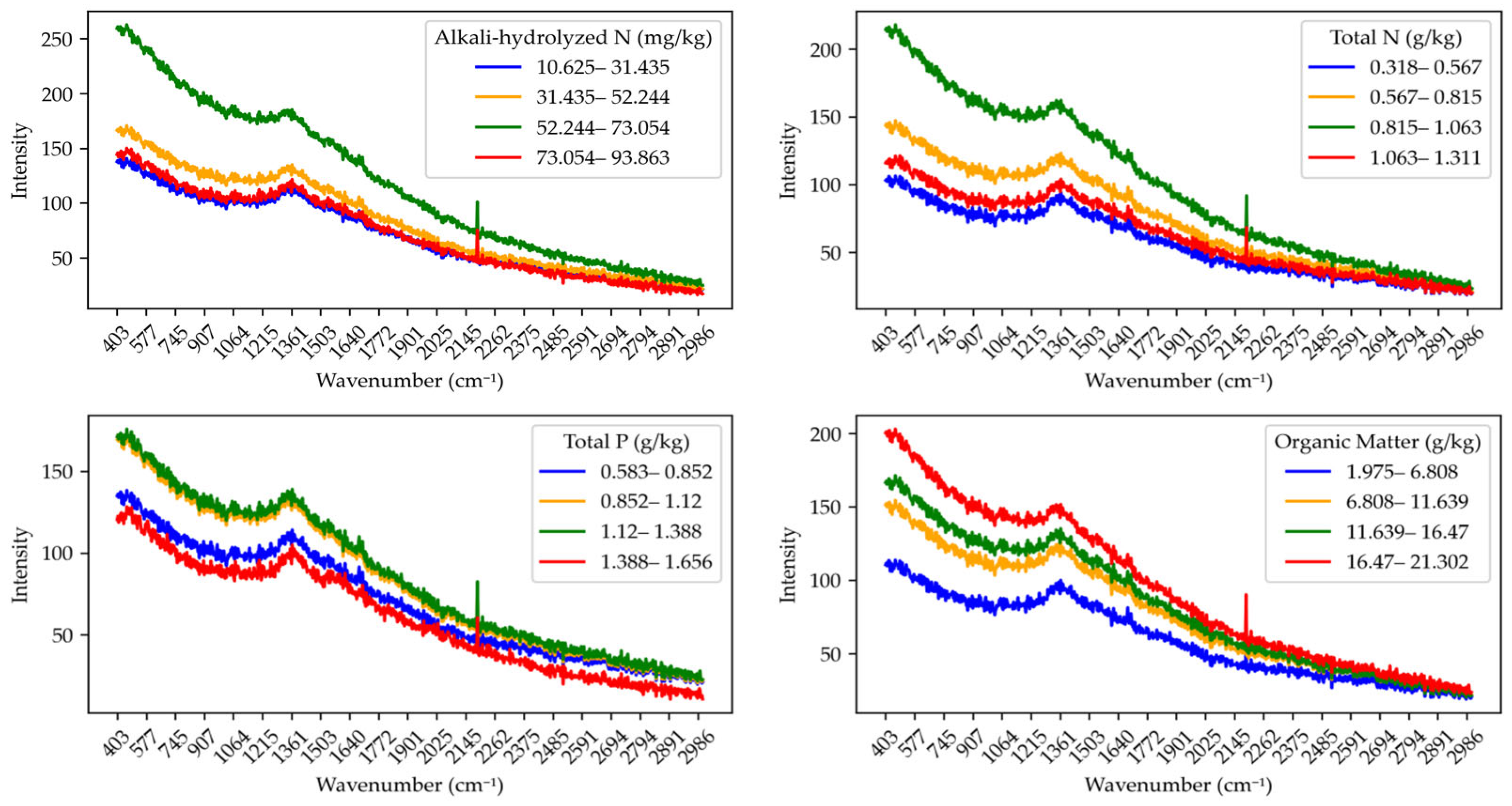
Figure 3 presents the raw Raman spectral curves of soil samples across different concentration intervals for each nutrient: alkali-hydrolyzed nitrogen, total nitrogen, total phosphorus, and organic matter. The four subfigures, respectively, show the spectral variation trends corresponding to these nutrients.

For alkali-hydrolyzed nitrogen, as the concentration increases, the Raman spectral intensity exhibits varying degrees of change, and distinct absorption characteristics emerge across different wavenumber ranges. The spectral differences between concentration intervals are pronounced, indicating that alkali-hydrolyzed content significantly influences the Raman response. Total nitrogen shows similar spectral characteristics to AN, but the variation across concentration intervals appears more gradual, suggesting a more regular influence of TN content on the Raman spectra. For total phosphorus, there are notable spectral differences across different concentration levels. As TP content increases, the overall spectral trend changes accordingly. The characteristic peaks of TP in the Raman spectra may occur at different wavenumber positions compared to other nutrients. Organic matter displays more complex spectral curves across different concentrations, indicating a strong spectral response in the Raman region. At higher organic matter levels, spectral intensity tends to increase.

Overall, the concentration variations in different nutrients produce distinct characteristic peaks in the Raman spectra, suggesting that each nutrient influences the spectral features in a unique manner. These spectral curves provide a basis for further feature extraction and analysis, supporting the quantitative prediction of soil nutrient contents.

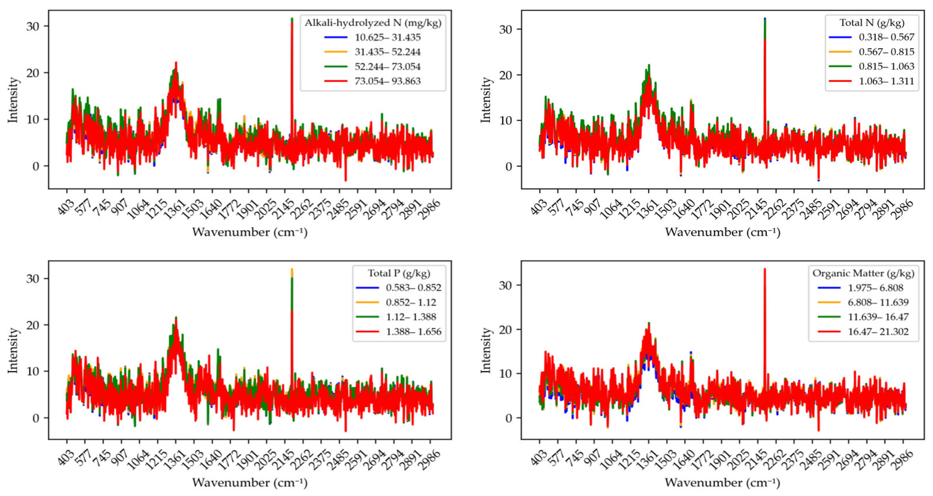
To reduce the impact of baseline drift and instrumental noise, baseline correction was performed, which aids subsequent quantitative analysis and feature extraction. The results of the baseline correction are shown in Figure 4. The Raman spectral curves of alkali-hydrolyzed nitrogen exhibit pronounced fluctuations, especially at higher concentrations (73.054–93.863 mg/kg), where the intensity values significantly increase, indicating greater sensitivity of the Raman response in this range. The spectral differences across concentration intervals further confirm that higher concentrations may present more absorption peaks in the Raman spectrum.

For total nitrogen, the spectral intensity shows different trends across concentration intervals (e.g., 0.318–0.567 g/kg, 0.567–0.815 g/kg). At lower concentrations (0.318–0.567 g/kg), the spectral curves are relatively flat, while at higher concentrations (1.063–1.311 g/kg), the curves reveal more spectral features, suggesting that high total nitrogen content may have a stronger influence on the Raman spectrum. Regarding total phosphorus, the spectral intensity at the same wavenumber varies significantly across different concentration intervals, especially at higher concentrations (1.388–1.656 g/kg), where the spectra display stronger absorption peaks. This indicates a more prominent contribution of TP to the Raman signal, with peak intensity increasing significantly at higher concentrations. The spectral variation in organic matter is more complex. Across different concentration intervals, the spectral intensity shows various fluctuation patterns. Overall, there are large differences in spectral intensity between low and medium organic matter concentration ranges, while the intensity is relatively stable at high concentrations. This may relate to the molecular structure and content of organic matter.

In summary, the baseline-corrected spectral data more clearly reveal the Raman spectral features of each nutrient across different concentration ranges. By comparing spectral variations among concentration intervals, a deeper understanding of the Raman response characteristics of soil nutrients can be achieved, thereby providing a reliable foundation for accurate quantitative analysis of soil nutrient contents.

3.3. Analysis of Spectral Preprocessing Results

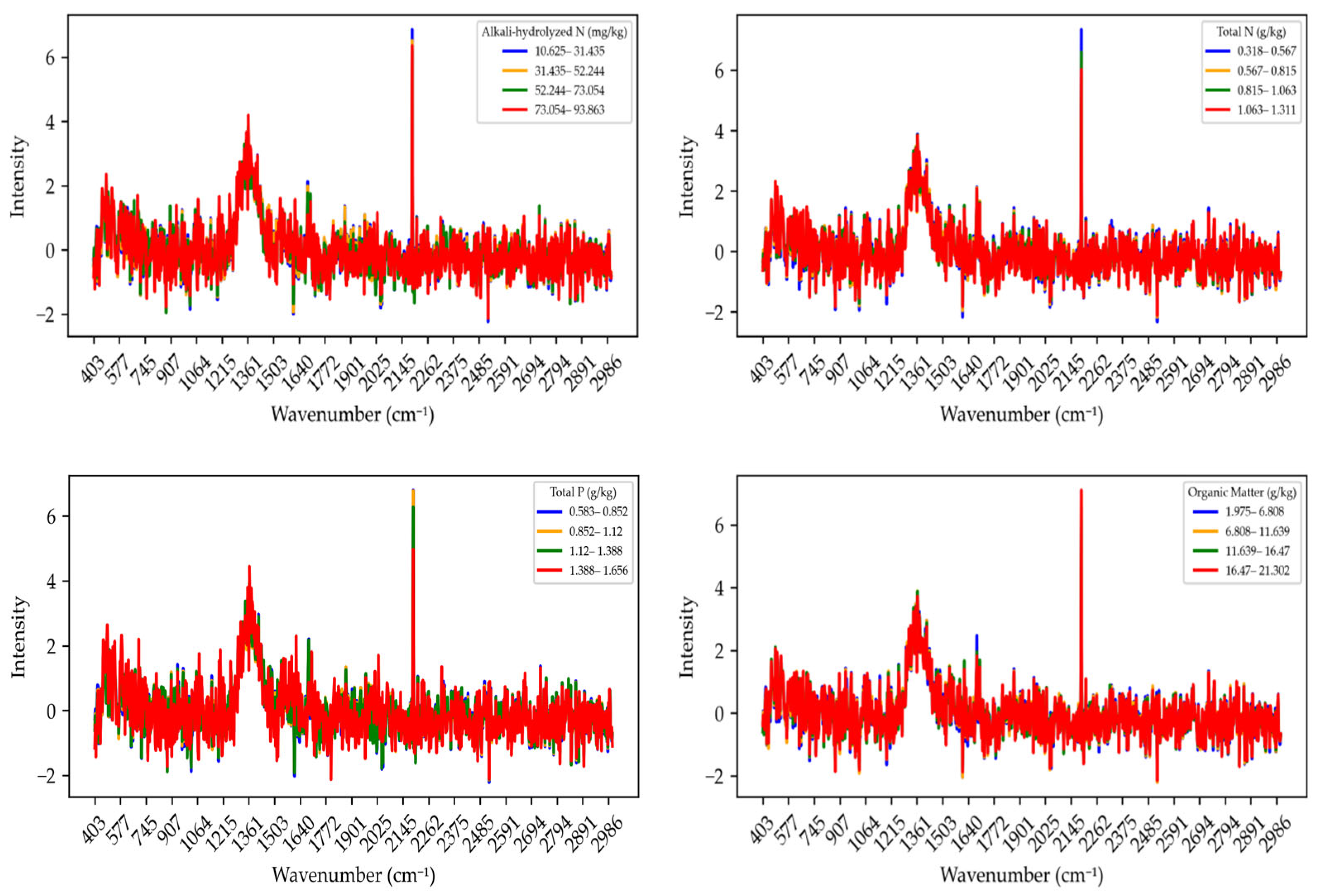
The Raman spectra of various soil nutrients processed using Raw_SNV (Standard Normal Variate) transformation after baseline correction are shown in Figure 5. Baseline correction eliminated baseline drift and instrumental noise in the spectra, making the association between the signal and target components more accurate. Subsequently, SNV processing was applied, which helps eliminate scattering differences between samples and further reduces the impact of external factors on the spectral signal. The Raw_SNV process made the spectral curves more consistent in shape, providing a more reliable foundation for subsequent quantitative analysis and feature extraction. After Raw_SNV processing, the Raman spectra of alkali-hydrolyzed nitrogen became smoother across different concentration intervals, removing spectral fluctuations caused by scattering effects. Notably, in higher concentration ranges (e.g., 73.054–93.863 mg/kg), the characteristic signals of the spectra became more distinct, and the intensity of certain absorption peaks was enhanced, possibly related to the molecular structure of alkali-hydrolyzed nitrogen. For total nitrogen, after Raw_SNV processing, the spectra across different concentration intervals (e.g., 0.318–0.567 g/kg, 0.567–0.815 g/kg, etc.) appeared smoother and more consistent. The processed curves exhibited prominent absorption peaks at specific wavelengths (such as around 1600 cm⁻¹), indicating a strong Raman response of total nitrogen at these positions. After Raw_SNV processing of total phosphorus samples, background noise in the spectra was significantly reduced, and spectral differences across different concentration intervals (e.g., 0.853–1.112 g/kg, 1.112–1.388 g/kg, etc.) became clearer. This indicates that Raw_SNV processing effectively improved the reliability of the signal, allowing the Raman response of total phosphorus to better reflect its concentration in the soil. For organic matter, Raw_SNV processing resulted in significantly increased signal differences between low and high concentration intervals. Particularly in the high concentration interval (16.47–21.302 g/kg), the absorption peaks of organic matter were prominent, indicating stronger Raman signal recognition ability at this range. In summary, baseline correction and Raw_SNV processing significantly improved the accuracy and comparability of the Raman spectra for each nutrient, providing a more reliable data basis for subsequent soil nutrient quantification and spectral feature extraction. These improvements not only enhanced the spectral responses across different concentration intervals but also laid a solid foundation for developing Raman spectroscopy-based soil nutrient detection methods.

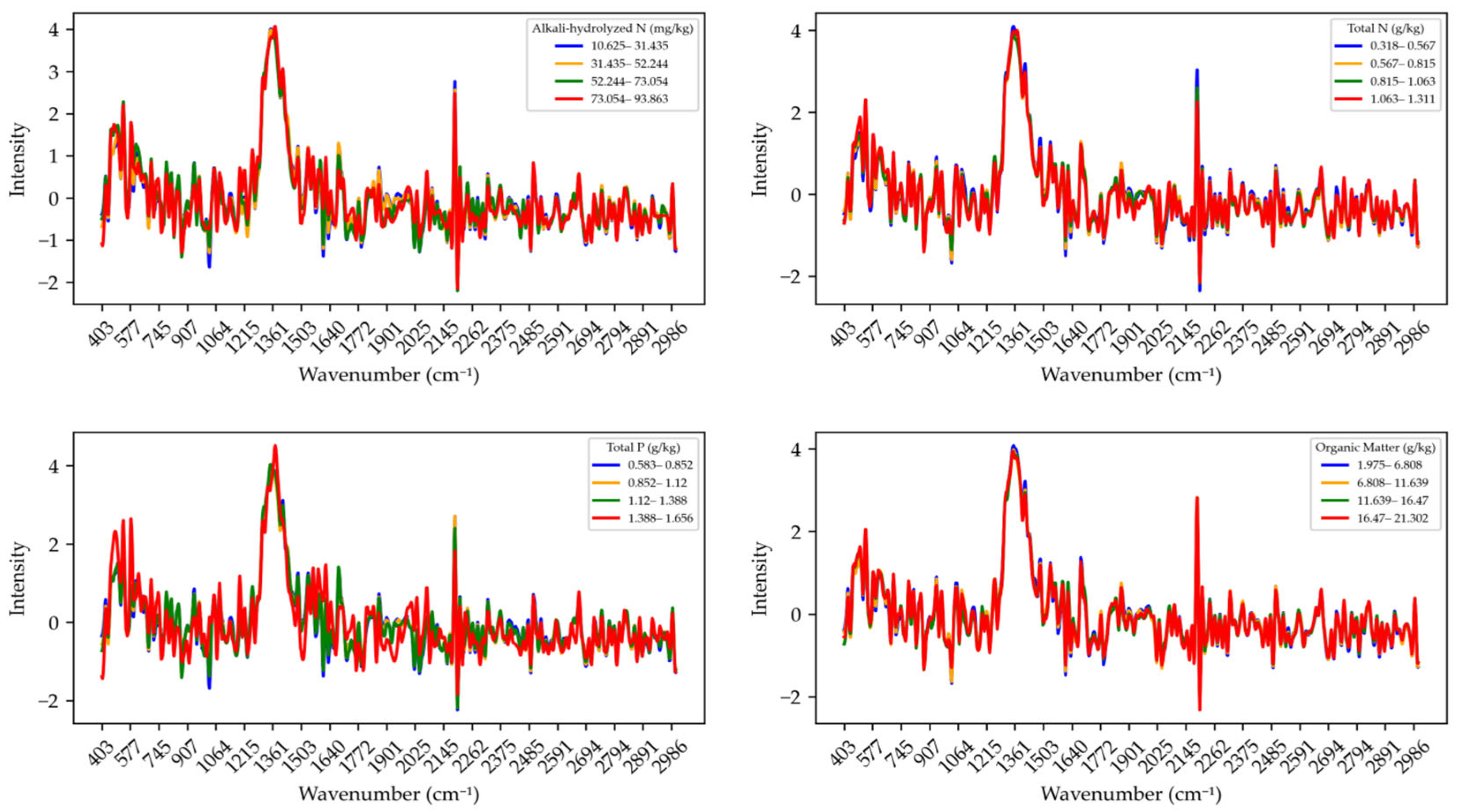
The Raman spectra of soil nutrients processed with SG_D1_SNV after baseline correction are shown in Figure 6. SG-D1 refers to the application of the Savitzky–Golay derivative filter, which removes noise and interference from the spectra, improving smoothness and enhancing the extraction of spectral features. Meanwhile, SNV (Standard Normal Variate) helps eliminate scattering effects among samples, making the spectra more consistent and improving the comparability of Raman signals. This preprocessing approach plays a key role in improving spectral quality and reducing the influence of external variables. For alkali-hydrolyzed nitrogen, after SG_D1_SNV processing, the spectral noise is significantly reduced, and in the range of 73.054–93.863 mg/kg, the characteristic peaks are more clearly expressed. The processed spectral curves show a more consistent trend, eliminating previous signal fluctuations and enhancing the effectiveness of feature extraction. For total nitrogen, the SG_D1_SNV-processed spectra become smoother, especially in the ranges of 0.318–0.567 g/kg and 0.567–0.815 g/kg, where the Raman signals appear more stable. Signal fluctuations across the wavelength range are significantly reduced, and certain key absorption peaks become more prominent. For total phosphorus, SG_D1_SNV processing enhances the spectral differences between different concentration intervals and improves signal comparability. Moreover, the characteristic peaks become more distinct, especially at specific wavenumbers, indicating the effectiveness of this method in the quantitative analysis of total phosphorus. For organic matter, the processed spectra exhibit a smoother trend. In particular, within the range of 16.47–21.302 g/kg, the absorption peaks are enhanced, and spectral noise is significantly suppressed, demonstrating the positive contribution of this method to the quantitative analysis of organic matter content.

Overall, SG_D1_SNV preprocessing significantly improves the quality and comparability of Raman spectra for different nutrients by removing noise, smoothing the curves, and reducing sample-to-sample scattering differences. It provides more reliable data support for subsequent quantitative analysis and modeling.

The Raman spectra of soil nutrients after wavelet denoising and SNV (Standard Normal Variate) preprocessing are shown in Figure 7. Wavelet transform is an effective signal denoising method, particularly suitable for removing high-frequency noise from spectra and producing smoother signals. Based on this, SNV preprocessing further eliminates inter-sample differences caused by light scattering effects, ensuring comparability between spectra of different samples and enhancing the prominence of key absorption peaks. For alkali-hydrolyzed nitrogen, after Wavelet_SNV processing, high-frequency noise in the spectral curves is effectively removed. Especially in low concentration (10.625–31.435 mg/kg) and high concentration (73.054–93.863 mg/kg) intervals, the curves become smoother, and the absorption peak positions are clearly visible. This processing method shows excellent denoising performance across different concentration levels, enabling more accurate identification of spectral features. For total nitrogen, Wavelet_SNV processing results in more consistent spectral curves across different concentration intervals. The method eliminates inter-sample scattering differences and enhances signal contrast, making the characteristic peaks more pronounced and consistent. For total phosphorus, the spectra after Wavelet_SNV processing display strong spectral features across different concentration ranges, with noise effectively removed. Particularly at specific wavenumber regions, absorption peaks are clearly defined and highly distinguishable, demonstrating the effectiveness of this method in spectral preprocessing. For organic matter, the spectra show significantly reduced noise after Wavelet_SNV processing. In higher concentration ranges (e.g., 16.47–21.302 g/kg), the signals become smoother, and the absorption peaks are more prominent, providing clearer spectral data for subsequent quantitative analysis.

Overall, after wavelet denoising and SNV normalization, the Raman spectral signals for various soil nutrients become smoother and clearer. Noise is significantly reduced, inter-sample scattering effects are effectively corrected, and spectral features are more consistent. This preprocessing method substantially improves model accuracy and data comparability in soil nutrient analysis, providing a more reliable data foundation for subsequent analysis and modeling.

Overall, the spectral curves corresponding to different nutrient levels exhibit noticeable variations in band positions and characteristic intensities, with some regions showing particularly prominent responses.

For alkali-hydrolyzed nitrogen (AN), clear intensity differences are observed in the regions of 670–730 cm⁻¹, 1250–1350 cm⁻¹, and 1550–1650 cm⁻¹, with a notably enhanced peak around ~1320 cm⁻¹. This may be attributed to C–N stretching vibrations or amino/amido functional groups (e.g., NH₄⁺, N–H) with Raman activity. These groups are commonly associated with readily available nitrogen forms, which are highly responsive in Raman spectra—explaining the relatively high modeling accuracy achieved for AN.

For total nitrogen (TN), the spectral variation trend resembles that of AN, with major response zones also concentrated in 1250–1350 cm⁻¹ and 1550–1650 cm⁻¹. However, the overall distinction between groups is less pronounced, indicating that while Raman spectroscopy can partially reflect the distribution of bioavailable nitrogen within TN, it has limited sensitivity to nitrogen bound in organic forms. Minor differences also appear around 1120–1180 cm⁻¹, which may relate to amine group vibrations.

For total phosphorus (TP), spectral curves show minimal differences among concentration groups, with only slight fluctuations near ~980 cm⁻¹ and ~1040 cm⁻¹. The former may correspond to the symmetric stretching vibration of PO₄³⁻, but the signal is weak—likely obscured by background interference and further affected by fluorescence, iron/aluminum oxide adsorption, and other soil matrix effects. These factors contribute to the unstable Raman response for TP, which aligns with the observed low prediction accuracy and high model variability.

For organic matter (OM), samples show a pronounced peak in the 1580–1620 cm⁻¹ region, corresponding to aromatic carbon skeletons (C=C) or unsaturated carbon structures. Additionally, changes around ~1360 cm⁻¹ and ~2900 cm⁻¹ may be attributed to C–H bending and C–H stretching vibrations, respectively. These bands are generally enhanced in high-OM groups, suggesting that Raman spectroscopy has good recognition ability for humic substances and organic polymers in soil.

3.4. Comparison of Prediction Performance Under Different Feature Selection Strategies

To clearly illustrate the prediction performance under different feature selection strategies, this study utilized three types of preprocessed spectral data (Raw_SNV, SG_D1_SNV, and Wavelet_SNV) and applied three feature selection methods: Recursive Feature Elimination (RFE), XGBoost feature importance, and Random Forest (RF) feature importance. Based on these feature sets, a total of 14 regression models were constructed, including Linear Regression, Ridge, Lasso, ElasticNet, BayesianRidge, Random Forest (RF), Extra Trees Regressor (ETR), Gradient Boosting Regressor (GBR), HistGradientBoosting Regressor (HistGBR), XGBoost, Support Vector Regression (SVR), KNN, Multi-Layer Perceptron (MLP), and Polynomial Regression (Poly2_LR), to predict four soil nutrient indicators: alkali-hydrolyzed nitrogen (AN), total nitrogen (TN), total phosphorus (TP), and soil organic matter (SOM).

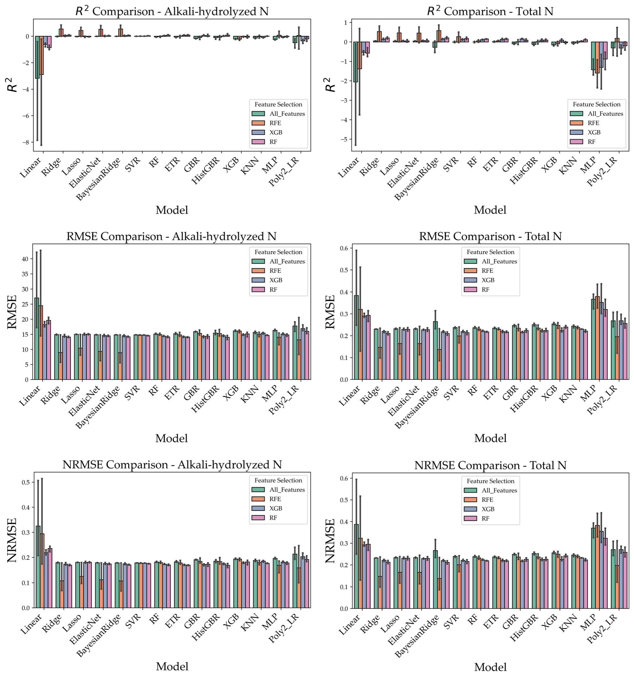
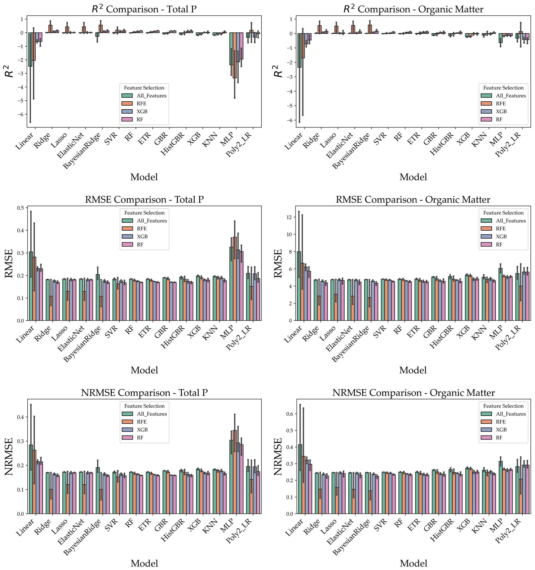
The predictive performance was comprehensively evaluated using R², RMSE, and NRMSE, and the results were visualized in Figure 8. Overall, the RFE feature selection method demonstrated the most superior and stable performance across most conditions. Particularly when combined with linear models such as ElasticNet and BayesianRidge, or ensemble models such as XGBoost and HistGBR, RFE significantly enhanced prediction accuracy, leading to higher R² values and lower RMSE and NRMSE values. For example, in the prediction of alkali-hydrolyzed nitrogen and soil organic matter, combinations of RFE with ElasticNet or XGBoost frequently achieved R² values above 0.80, with corresponding NRMSE values ranging from 0.10 to 0.20, outperforming other feature selection strategies.

In contrast, the RF-based feature selection method yielded reasonably good results in some models but lacked stability, exhibiting larger variability. The XGBoost-based feature selection method performed slightly better than RF in certain cases but was still generally inferior to RFE. Taken together, these findings suggest that RFE combined with ensemble learning models represents the optimal strategy for predicting soil nutrient indicators in this study.

Therefore, considering both predictive accuracy and robustness, RFE is validated as the most effective feature selection method for Raman spectroscopy-based soil nutrient modeling.

3.5. Comparative Analysis of Prediction Performance Across Different Data Preprocessing Methods

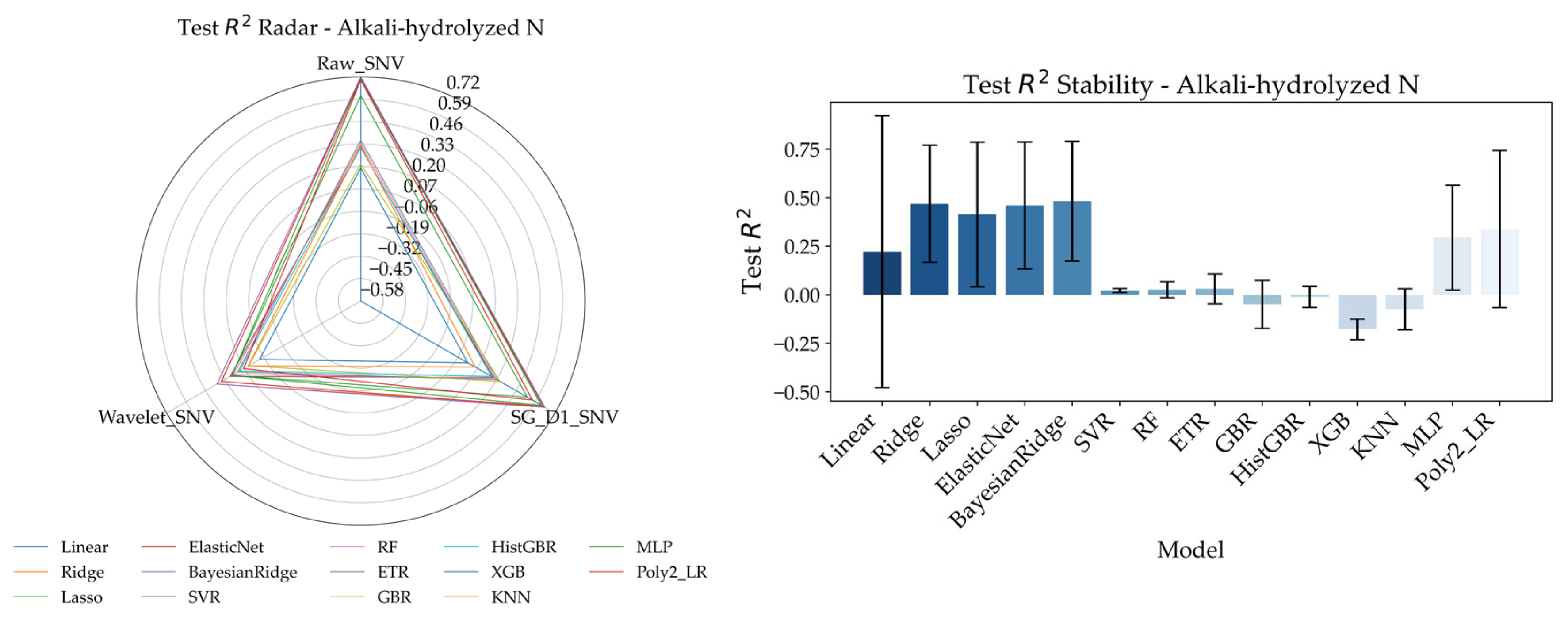
Based on RFE feature selection, this section further analyzes the performance of various models in predicting soil nutrients (alkali-hydrolyzed nitrogen, total nitrogen, total phosphorus, and organic matter) under different data preprocessing methods (Raw_SNV, Wavelength_SNV, SG_D1_SNV), as shown in Figure 9. Radar Charts are used to visualize the trends of model performance across different nutrients under various preprocessing strategies, while bar charts highlight the stability of each model under different data treatments. For alkali-hydrolyzed nitrogen prediction, the Radar Chart shows that models using Raw_SNV preprocessing (e.g., BayesianRidge, Ridge, ElasticNet) exhibit relatively stable performance with higher Test R² values. In contrast, models using SG_D1_SNV and Wavelength_SNV preprocessing perform slightly worse, indicating that Raw_SNV is more suitable for alkali-hydrolyzed nitrogen prediction. According to the bar chart, ElasticNet and BayesianRidge maintain high stability across all preprocessing methods, demonstrating consistent performance. In comparison, the SVR model shows greater performance fluctuations, especially with SG_D1_SNV and Wavelength_SNV preprocessing, where its performance significantly declines. For total nitrogen prediction, the Radar Chart indicates that different preprocessing methods have a more significant impact. Under Raw_SNV, most models (e.g., ETR, ElasticNet, BayesianRidge) achieve better Test R² values, while models trained on Wavelength_SNV and SG_D1_SNV treated data underperform. The bar chart further reveals that ElasticNet maintain higher stability, particularly under Raw_SNV and SG_D1_SNV, showing strong robustness in handling total nitrogen data. Other models, such as SVR and XGB, exhibit larger fluctuations, with XGB performing poorly under Wavelength_SNV preprocessing. For total phosphorus prediction, the Radar Chart shows that all models perform relatively well under Raw_SNV, especially ElasticNet and BayesianRidge. Wavelength_SNV and SG_D1_SNV preprocessing, however, result in less satisfactory outcomes, suggesting that Raw_SNV provides a clear advantage for phosphorus prediction. In the bar chart, ElasticNet maintain high stability across all preprocessing methods, with consistent Test R² values. Other models show considerable variability, particularly under SG_D1_SNV, where performance significantly drops. For organic matter prediction, the Radar Chart reveals similar performance between Raw_SNV and SG_D1_SNV, with ElasticNet and BayesianRidge achieving higher Test R² values. Wavelength_SNV performs less effectively, indicating that Raw_SNV is better suited for organic matter prediction. In the bar chart, ElasticNet and BayesianRidge demonstrate the highest stability under all preprocessing methods, while models such as KNN and SVR exhibit lower stability, particularly under Wavelength_SNV where performance sharply declines.

Overall, the Raw_SNV preprocessing method generally yields more stable and accurate results, especially in predicting alkali-hydrolyzed nitrogen, total nitrogen, and organic matter. Wavelength_SNV and SG_D1_SNV have variable effects depending on nutrient type and model characteristics. Additionally, ElasticNet and BayesianRidge consistently demonstrate superior stability and predictive performance, making them highly recommended models for Raman spectroscopy-based soil nutrient prediction.

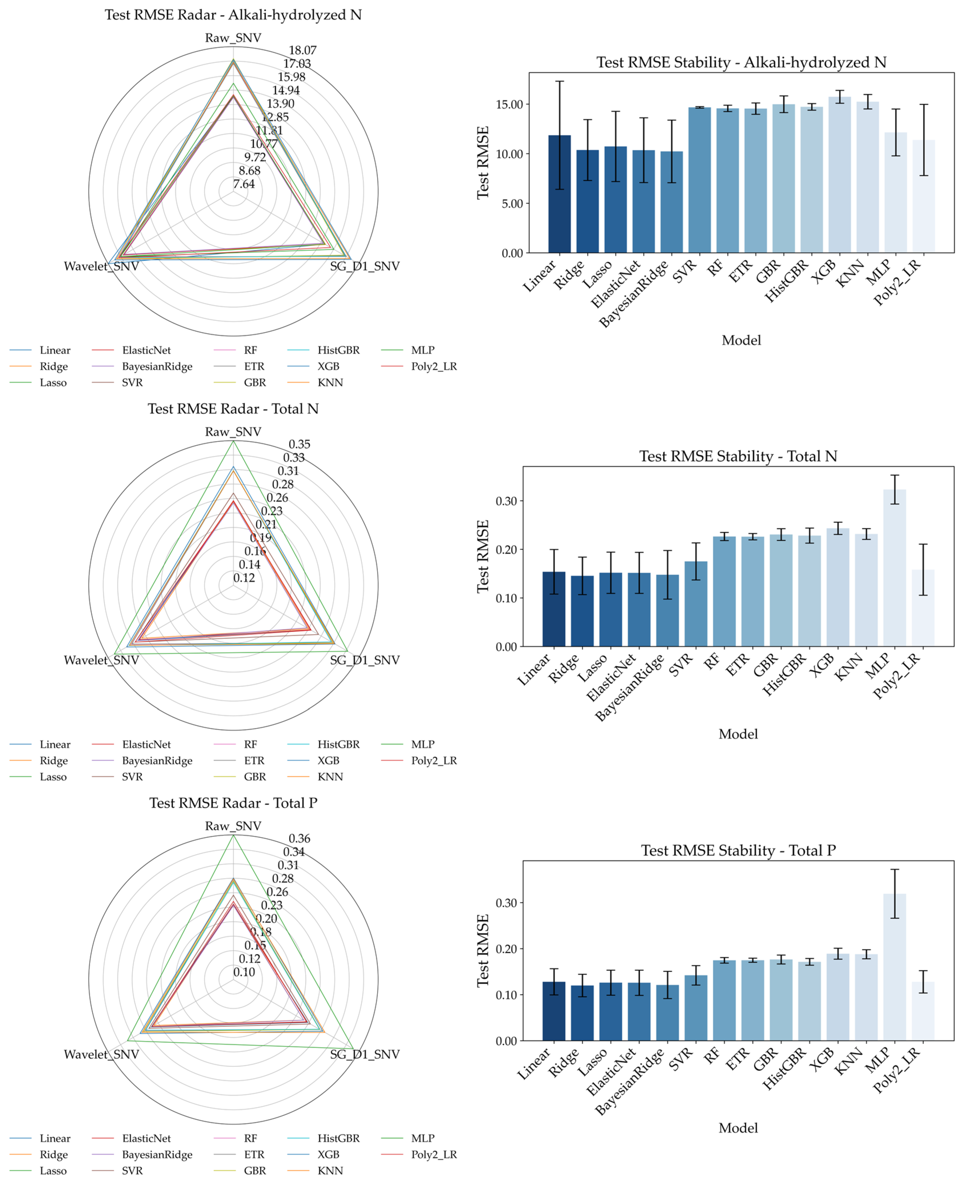
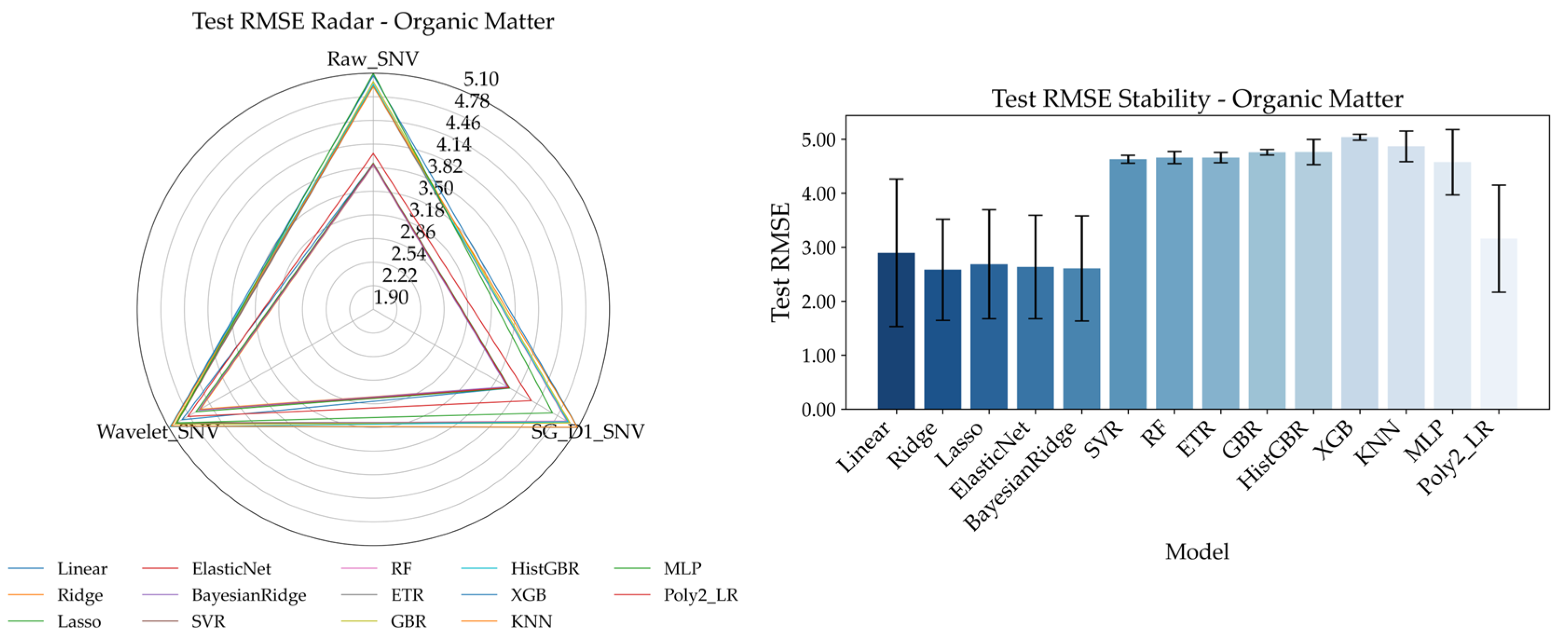
To systematically evaluate the performance of different spectral preprocessing methods and regression models in predicting soil nitrogen, phosphorus, and organic matter, the results are shown in Figure 10. Figure 10 presents Radar Chart of Test RMSE (left) and bar charts of prediction stability (right) for the four soil nutrient indicators under three spectral preprocessing methods (Raw_SNV, Wavelet_SNV, SG_D1_SNV), providing a comprehensive reflection of the predictive performance differences across various preprocessing and modeling schemes.

From the Radar Chart, one can observe the RMSE variation trends of different models for the same indicator under each preprocessing method. Among the three preprocessing methods, Raw_SNV (raw spectrum + Standard Normal Variate transformation) exhibits a generally narrower RMSE range across most models, indicating lower prediction error and higher stability. For alkali-hydrolyzed nitrogen and organic matter, Raw_SNV performs significantly better than the other methods; for total nitrogen and total phosphorus, while the differences are slightly smaller, Raw_SNV still generally outperforms the others. Therefore, Raw_SNV is considered the most universally applicable preprocessing scheme across the four nutrient indicators, laying a solid foundation for subsequent model performance evaluations. Based on Raw_SNV, the bar charts display the average RMSE and standard deviation under 5-fold cross-validation for each regression model, used to assess prediction accuracy and stability: alkali-hydrolyzed nitrogen achieves lower RMSE in BayesianRidge and Ridge, with BayesianRidge showing smaller standard deviation and thus better consistency. Organic matter yields the lowest errors under Raw_SNV. ETR demonstrating stronger robustness. Total nitrogen performs well with GBR (Gradient Boosting Regressor), BayesianRidge, and ETR, among which GBR balances error and stability effectively. Total phosphorus shows excellent performance with BayesianRidge and ElasticNet, with BayesianRidge in particular offering advantages in both error reduction and variance control.

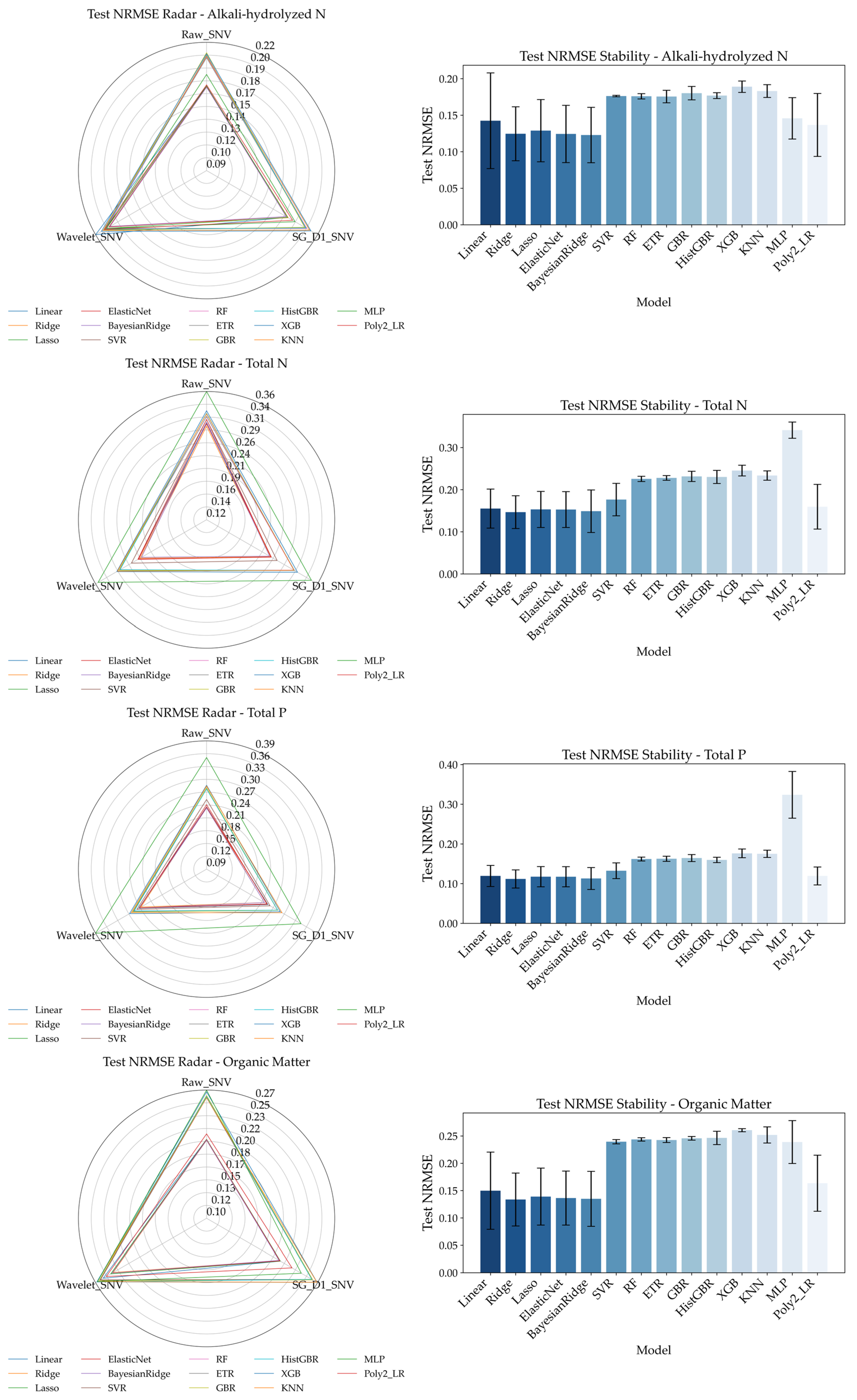
To further evaluate the impact of different combinations of spectral preprocessing methods and regression models on the prediction of soil nutrient indicators, Figure 11 presents the validation set NRMSE performance after RFE-based feature selection. NRMSE (normalized root mean square error) serves as a key metric to quantify the relative prediction error of models—the lower the NRMSE, the higher the prediction accuracy and generalization capability. To clarify the performance differences, the left side of the figure shows Radar Chart of model NRMSEs under different preprocessing methods, while the right side presents bar charts illustrating the stability of each model’s NRMSE averaged across the three preprocessing methods.

From an overall perspective, spectral preprocessing methods have a significant impact on the predictive accuracy of the models. Among them, the Raw_SNV preprocessing consistently delivers the best NRMSE results across all four soil indicators, effectively enhancing model generalization—particularly in the prediction of alkali-hydrolyzed nitrogen (AN) and total nitrogen (TN) where the advantages are most pronounced. Wavelet_SNV ranks second, maintaining relatively low errors especially in AN prediction. In contrast, SG_D1_SNV often leads to increased prediction errors, performing worse than the other two methods, suggesting that it may introduce excessive signal noise, which is detrimental to modeling.

From the perspective of model performance, linear- and regularization-based models (e.g., Ridge, BayesianRidge, ElasticNet) tend to produce lower NRMSE values with higher stability, showing robust performance particularly in AN and TN prediction. On the other hand, more complex nonlinear models (e.g., XGBoost, KNN, MLP) may occasionally yield excellent results but are accompanied by larger error bars, indicating higher sensitivity to data and lower stability. Taking AN as an example, although XGBoost and HistGBR achieve relatively good performance under certain preprocessing methods, their large standard deviations reflect substantial uncertainty. In contrast, Ridge and BayesianRidge consistently remain within a low error and low variance range.

In terms of prediction difficulty, alkali-hydrolyzed nitrogen is the easiest to predict, with the lowest overall NRMSE (<0.15) and minor differences across models—suggesting a strong correlation with spectral features. Total nitrogen follows, with slightly higher NRMSE values but similar trends. In contrast, total phosphorus and organic matter are evidently more challenging to predict, showing higher average NRMSE values (approximately 0.20–0.35 for TP and 0.15–0.25 for OM) and greater variability across models, indicating a more complex relationship with spectral signals or the influence of non-spectral factors.

3.6. Model Prediction Error Analysis

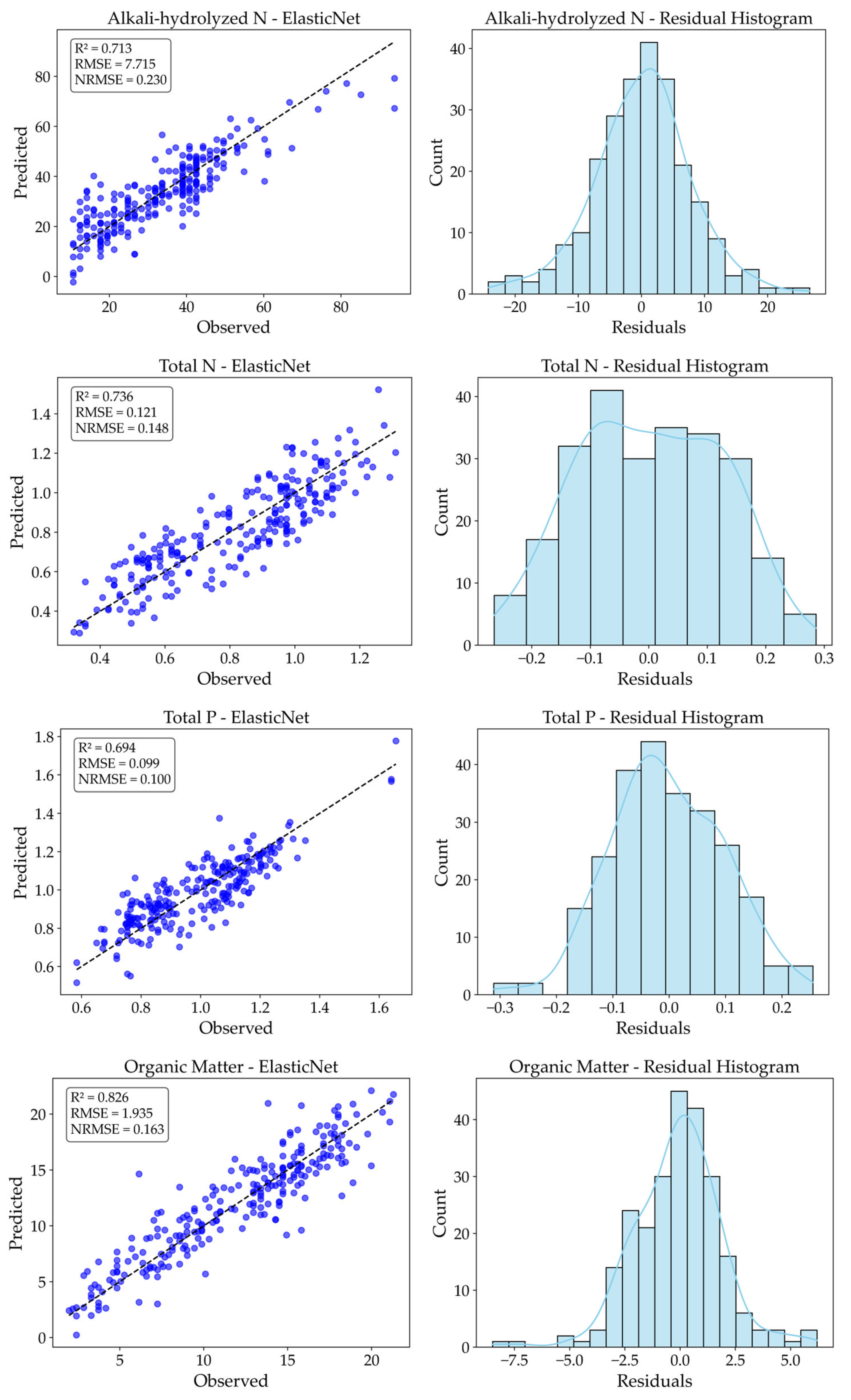
To comprehensively evaluate the predictive performance of the model, an error analysis was conducted on the ElasticNet regression results for the four types of soil nutrients, as shown in Figure 12. The results demonstrate that the ElasticNet model performs stably across all four nutrient components, exhibiting good fitting accuracy and residual distribution characteristics.

Among them, the prediction results for alkali-hydrolyzed nitrogen (AN) and organic matter (OM) are relatively better. The scatter plots show high consistency between the predicted and observed values, with the fitted line closely aligned with the 45° reference line. The R² values reach 0.713 for AN and 0.826 for OM, and the corresponding NRMSE values are 0.230 and 0.163, respectively. The residual histograms exhibit near-normal distributions, indicating small and unbiased errors, thus confirming the models’ stable and reliable prediction performance.

The prediction of total nitrogen (TN) ranks second, with an R² of 0.736 and NRMSE of 0.148. Although slight deviation is observed in the residuals, the overall prediction error remains low, making it suitable for quantitative estimation and monitoring under laboratory conditions.

For total phosphorus (TP), the prediction performance is slightly lower with an R² of 0.694 and NRMSE of 0.100. While it still possesses a certain degree of predictive accuracy, the scatter plot reveals relatively larger deviations for some samples. The residual histogram shows mild skewness, likely caused by variability at low concentration levels. Therefore, for indicators like TP with narrow value ranges and low signal intensity, introducing nonlinear regressors or ensemble learning strategies may further enhance model robustness and stability.

Overall, the current ElasticNet-based model demonstrates promising practical utility in predicting multiple soil nutrient parameters based on Raman spectroscopy and holds potential for broader applications in precision agriculture and intelligent soil monitoring.

4. Discussion

This study established predictive models for four soil nutrient indicators—alkali-hydrolyzed nitrogen (AN), total nitrogen (TN), total phosphorus (TP), and organic matter (OM)—based on Raman spectroscopy, and systematically evaluated the performance differences among various spectral preprocessing methods, feature selection strategies, and regression algorithms. The results demonstrate that Raman spectroscopy shows promising potential for non-destructive prediction of soil nutrients, particularly in modeling AN and OM with relatively high accuracy. However, several limitations and areas for improvement remain before practical deployment.

First, among the three compared spectral preprocessing methods, Standard Normal Variate (SNV) consistently delivered the most stable performance across all nutrient targets. Direct application of SNV to raw spectra (Raw_SNV) achieved the lowest normalized root mean square error (NRMSE), with combinations such as Raw_SNV + ElasticNet or BayesianRidge showing robust performance for AN and TN. In contrast, the Savitzky–Golay first derivative with SNV (SG_D1_SNV) introduced more noise in TP and OM predictions, resulting in greater model volatility and higher NRMSE values. This suggests the method’s sensitivity to minor spectral fluctuations may amplify noise.

Second, in feature selection, Recursive Feature Elimination (RFE) outperformed tree-based importance methods (e.g., XGBoost, Random Forest) for all nutrient predictions, especially for AN and OM. RFE combined with ElasticNet or BayesianRidge achieved high R² and low NRMSE, indicating its superior ability to identify key Raman bands highly correlated with nutrient concentrations. In comparison, tree-based methods retained more redundant features, increasing model variance and reducing the stability of TN and TP predictions.

Third, in terms of modeling algorithms, ElasticNet and BayesianRidge showed greater robustness, with lower standard deviations in error and higher R² values. Nonlinear models such as SVR and KNN exhibited larger errors, particularly for TP and OM, likely due to dimensional redundancy and overfitting. Ensemble models (e.g., XGBoost, HistGradientBoosting) performed well in certain cases but showed significant fluctuation for TP and OM, limiting their generalizability. The relatively high prediction accuracy of AN and TN may be attributed to their spectral responsiveness. AN represents the readily mineralizable or plant-available nitrogen forms, which often exhibit distinctive Raman-active signals (e.g., NH₄⁺, NO₃⁻, and C–N bonds). While TN includes both organic and inorganic nitrogen forms, there is usually a degree of correlation between the two. Raman spectroscopy can reflect structural information of both, but AN is more indicative of bioavailable nitrogen, thus its superior prediction performance partly reflects the technique’s higher sensitivity to readily labile functional groups. The lower accuracy for TP prediction may stem from the weaker intrinsic Raman response of phosphorus, as well as its complex occurrence forms in soil. Factors such as iron/aluminum oxides, soil texture heterogeneity, and fluorescent background noise further hinder TP signal extraction. Consequently, TP modeling exhibited higher NRMSE values and lower stability.

Regarding sample handling, the soil type in this study was cambisol, with samples collected from two depth layers (0–0.2 m and 0.2–0.4 m) to reflect potential vertical nutrient differences. The current models did not stratify predictions by soil layer; future work should investigate depth-specific effects on prediction accuracy and consider stratification as a key metric for evaluating model generalizability.

Despite the promising modeling framework established in this study, several limitations remain. First, all experiments were conducted under laboratory conditions, and the soil sampling scope was geographically limited. The current models were not developed separately for different soil layers; in future work, the impact of soil depth on prediction performance should be further investigated and considered as a key indicator for evaluating model generalizability. Factors such as soil moisture, heterogeneity, and environmental noise may reduce model performance in real field applications. Future studies should validate the models across broader regions and under real-time sensing scenarios. Second, although RFE effectively reduced feature dimensionality, Raman spectra remain high-dimensional and noise-prone. Residual redundancy can still affect model generalization. Future efforts may explore advanced optimization techniques such as multi-objective genetic algorithms or deep learning-based feature extraction (e.g., AutoEncoder, 1D-CNN) [60,61]. Third, this study employed a single-target modeling approach. However, soil nutrients often exhibit correlated dynamics. Multi-task learning frameworks [62] could enhance modeling efficiency by leveraging shared spectral representations for concurrent nutrient prediction. Finally, challenges related to sensor portability, measurement stability, and field integration must be addressed for large-scale deployment. Coupling Raman spectroscopy with portable devices and integrating contextual soil parameters (e.g., pH, moisture) could pave the way for real-time diagnostics in precision agriculture [63].

A key limitation for Raman-based soil analysis lies in the lack of global-scale spectral databases. Unlike visible–near-infrared (Vis-NIR) spectroscopy, which benefits from large, harmonized databases such as LUCAS [64], Raman spectroscopy suffers from poor standardization across instruments and sampling conditions [63]. Vis-NIR platforms have been widely applied to model soil texture, pH, CEC, and nutrient availability, whereas Raman spectral datasets remain fragmented and highly sensitive to fluorescence interference, particle size, and sample preparation protocols [65].

Moreover, algorithm development for Vis-NIR is more mature, and many models exhibit good transferability across soils and regions. In contrast, Raman models require further adaptation to handle high dimensionality, low signal-to-noise ratio, and strong background effects [63,66,67]. To overcome these limitations, future initiatives should focus on instrument calibration, open access Raman databases, and multi-modal data fusion to enhance model robustness and global applicability.

5. Conclusions

This study established a Raman spectroscopy-based soil nutrient prediction framework that integrates multiple spectral preprocessing methods, feature selection techniques, and regression modeling strategies. It systematically assessed the applicability and stability of the framework in predicting four soil indicators: alkali-hydrolyzed nitrogen, total nitrogen, total phosphorus, and organic matter. The results revealed that Recursive Feature Elimination (RFE) consistently outperformed XGBoost and Random Forest-based importance selection methods, offering superior stability and generalization capability in most scenarios. Standard Normal Variate (SNV) preprocessing, particularly in the Raw_SNV form, yielded the lowest NRMSE and highest R² across different nutrient indicators, making it one of the most effective spectral transformation approaches.

In terms of model performance, regularized linear models such as ElasticNet and BayesianRidge demonstrated excellent predictive accuracy and stability across multiple targets. Although ensemble models like XGBoost and HistGBR achieved top R² in specific cases, their performance was more variable, suggesting that they are better suited to high-quality datasets with careful parameter tuning.

Regarding the predictability of different indicators, alkali-hydrolyzed nitrogen showed the strongest spectral response and lowest modeling error, making it the most reliably predicted nutrient. Total nitrogen followed, while total phosphorus and organic matter were more difficult to predict due to the influence of non-spectral factors, reflected in higher errors and greater variability.

In summary, this study validates the effectiveness and application potential of Raman spectroscopy combined with RFE and SNV preprocessing for accurate and low-disturbance soil nutrient prediction, particularly in dryland regions. The proposed framework offers a practical technical pathway and theoretical foundation for precision agriculture and digital soil nutrient monitoring.