LiDAR-IMU Sensor Fusion-Based SLAM for Enhanced Autonomous Navigation in Orchards

Abstract

Labor shortages and uneven terrain in orchards present significant challenges to autonomous navigation. This study proposes a navigation system that integrates Light Detection and Ranging (LiDAR) and Inertial Measurement Unit (IMU) data to enhance localization accuracy and map stability through Simultaneous Localization and Mapping (SLAM). To minimize distortions in LiDAR scans caused by ground irregularities, real-time tilt correction was implemented based on IMU feedback. Furthermore, the path planning module was improved by modifying the Rapidly-Exploring Random Tree (RRT) algorithm. The enhanced RRT generated smoother and more efficient trajectories with quantifiable improvements: the average shortest path length was 2.26 m, compared to 2.59 m with conventional RRT and 2.71 m with A* algorithm. Tracking performance also improved, achieving a root mean square error of 0.890 m and a maximum lateral deviation of 0.423 m. In addition, yaw stability was strengthened, as heading fluctuations decreased by approximately 7% relative to the standard RRT. Field results validated the robustness and adaptability of the proposed system under real-world agricultural conditions. These findings highlight the potential of LiDAR–IMU sensor fusion and optimized path planning to enable scalable and reliable autonomous navigation for precision agriculture.

1. Introduction

In recent decades, agricultural productivity has steadily increased, largely driven by technological advancements and rising global food demand [1,2]. However, this upward trend obscures growing concerns about long-term sustainability. Rural populations are aging, and younger generations show diminishing interest in agricultural labor, resulting in chronic workforce shortages [3,4]. These challenges are particularly pronounced in orchard farming, where labor-intensive activities—such as pruning, harvesting, and pest control—require both skill and consistency, making them highly susceptible to fluctuations in labor supply [5]. To address these issues, agricultural robotics has emerged as a promising solution. Autonomous systems capable of performing high-value tasks, including fruit harvesting, crop monitoring, and pesticide application, offer significant potential to improve labor efficiency in orchards growing apples, grapes, and other premium crops [6,7]. Despite advancements in robotic hardware for mobility and manipulation, reliable autonomous navigation in unstructured orchard environments remains a major technical challenge. Irregular terrain, dense foliage, and narrow rows hinder accurate localization and consistent path tracking [8,9].

Accurate localization is essential for reliable autonomous navigation. Although Real-Time Kinematic Global Navigation Satellite System (RTK-GNSS) offers centimeter-level accuracy in open fields, its performance deteriorates significantly under orchard canopies due to signal occlusion [10,11]. Vision-based localization methods provide rich spatial data but are highly sensitive to lighting and weather variability, which limits their reliability in outdoor environments [12,13]. In contrast, Light Detection and Ranging (LiDAR) offers high-precision, lighting-independent distance measurements, making it well-suited for complex navigation tasks [14,15]. Two-dimensional (2D) LiDAR is widely used for row detection and obstacle avoidance due to its simplicity and low computational cost [16,17]. However, its inability to detect elevation changes restricts its application in uneven or sloped terrains [18]. To overcome this limitation, researchers have explored the integration of three-dimensional (3D) LiDAR with Simultaneous Localization and Mapping (SLAM), which enhances spatial perception but also increases computational and energy demands [19,20]. Sensor fusion—particularly the integration of LiDAR with Inertial Measurement Unit (IMU) data—has gained traction as a strategy to enhance localization accuracy while maintaining computational efficiency. IMUs can detect pitch and roll deviations, enabling correction of tilt-induced LiDAR scans distortions and improving pose estimation [21,22]. Recent research has demonstrated that LiDAR–IMU fusion significantly reduces drift and improves map stability in rugged agricultural terrains [23,24]. Hong et al. (2024) demonstrated robust 3D localization in agricultural scenes by introducing a hierarchically coupled LiDAR–inertial odometry framework [25]. Kim et al. (2024) proposed a covariance-intersection-based SLAM approach that significantly improved positioning accuracy in outdoor fields [26]. Wang et al. (2024) advanced LVI-SAM to enhance the localization performance of mobile robots operating in cluttered conditions [27]. Ban et al. (2024) integrated Camera–LiDAR–IMU fusion to enable reliable real-time crop-row navigation [28], while Chen et al. (2025) introduced a LiDAR-based centreline navigation method specifically tailored for orchard environments [29].

Path planning also plays a pivotal role in autonomous navigation. Classical algorithms, such as A* and Dijkstra, often perform poorly in dense, cluttered environments due to their rigid structure and computational inefficiency [30]. In contrast, sampling-based methods, including Rapidly-Exploring Random Tree (RRT) and its enhanced variant (RRT*), offer greater flexibility and adaptability for complex path generation [31]. Extensions, such as Quick-RRT* and Bidirectional RRT, further improve smoothness and obstacle avoidance in constrained orchard layouts [32]. Effective path tracking is equally important. The Pure Pursuit algorithm, widely adopted in agricultural robotics for its simplicity and real-time responsiveness, has recently been refined to better handle sharp turns and uneven terrain—conditions typical of orchard settings [33,34].

Building on these advancements, this study develops and evaluates a LiDAR–IMU fusion-based autonomous navigation system specifically designed for orchard environments. The primary objectives of the study are (1) to enhance localization accuracy by integrating LiDAR and IMU data for robust pose estimation in uneven and unstructured terrains and (2) to validate the navigation performance of the proposed system through a comprehensive evaluation framework, including simulations in Gazebo, controlled indoor experiments, and field trials in real orchard settings. These objectives support the development of a scalable and practical navigation solution for precision agriculture under complex field conditions.

2. Materials and Methods

2.1. Simulation Experiment Design

2.1.1. Robot Platform and Sensor Modeling

The SCOUT 2.0 mobile platform (AgileX Robotics, Shenzhen, China) was implemented in the Gazebo simulation environment using XML Macros (XACRO), which offer greater modularity and reusability than the traditional Unified Robot Description Format (URDF). The SCOUT_v2.xacro configuration accurately captured the robot’s physical characteristics, including linkages, joints, mass properties, and collision boundaries, thereby enabling realistic kinematic and dynamic behavior in the simulation. For perception modeling, a Velodyne VLP-16 LiDAR sensor (Velodyne Lidar, San Jose, CA, USA) was centrally mounted at 0.45 m above ground level to provide 360° horizontal scanning for obstacle detection and environmental mapping. Additionally, a custom IMU model was incorporated at a height of 0.25 m and connected through the imu_link frame. This simulated IMU, specifically developed for Gazebo, was configured solely for yaw estimation. Sensor frames were precisely defined within the XACRO file to ensure accurate spatial alignment and consistency with real-world hardware configurations. The complete SCOUT 2.0 simulation model with mounted sensors is illustrated in Figure 1a. Figure 1b presents the visualization of the LiDAR point cloud, which exhibits high density and spatial coherence, confirming the effectiveness of the sensor setup for navigation-related tasks.

2.1.2. Simulation Software and ROS Configuration

The navigation system was developed using the Robot Operating System (ROS) Melodic Morenia, which served as the core middleware for data communication, motion planning, and actuator control. Each sensor was managed by a dedicated ROS node, with data exchanged through the publisher–subscriber mechanism. LiDAR point cloud data were published on the /velodyne_points topic, while orientation data from the IMU were transmitted through the /imu/data topic. The robot_state_publisher package (version 1.14.0, Open Source Robotics Foundation, Mountain View, CA, USA) and transformation libraries were employed to maintain real-time coordinate transformations between reference frames, enabling the seamless integration of sensor inputs for SLAM and localization processes. Global path planning was executed using the A* and RRT algorithms, while the Dynamic Window Approach (DWA) was implemented for local path planning and real-time obstacle avoidance. All components were organized within a modular ROS package structure, ensuring reusability, consistency, and scalability across both simulation and real-world deployment. This architecture enabled effective coordination among sensing, planning, and control modules, facilitating seamless transitions across all development stages.

2.1.3. Simulation Environment Setup

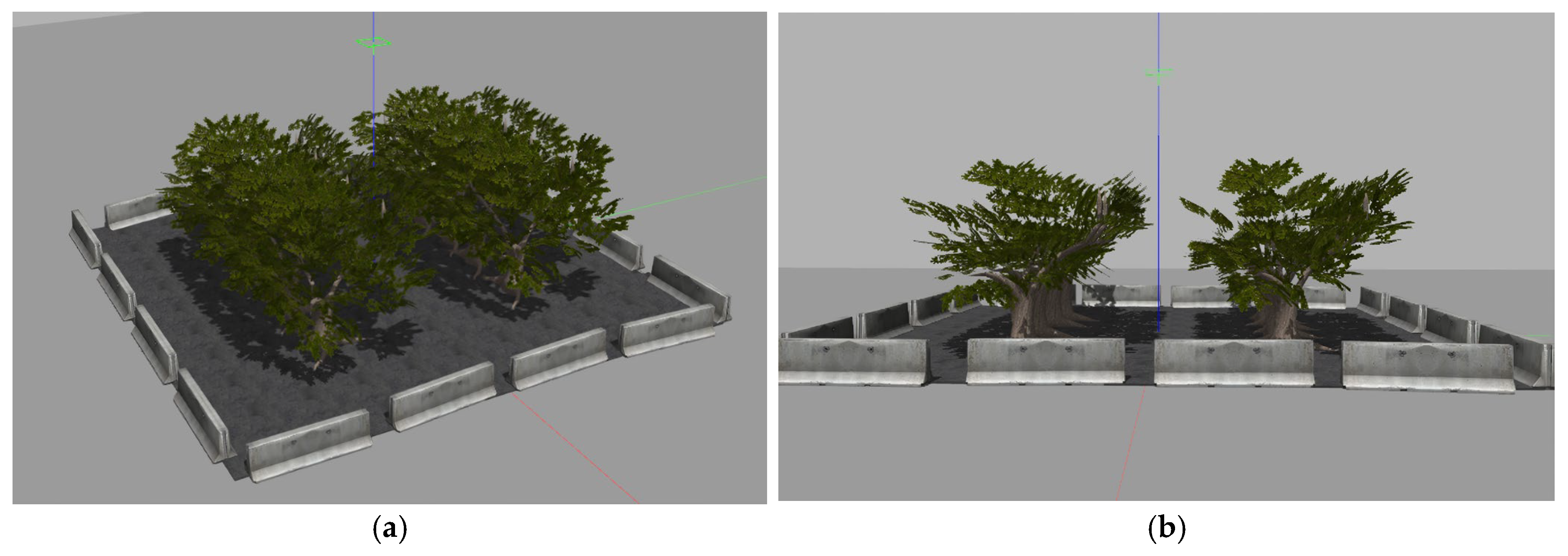
The simulation environment was constructed in Gazebo to replicate orchard-like conditions, enabling a realistic assessment of autonomous navigation performance. The virtual test field covered a 20 m × 20 m area and incorporated key orchard features, including tree rows, narrow pathways, and non-uniform terrain, to mimic real-world agricultural challenges (Figure 2). Eight tree models were strategically positioned to form structured navigation lanes. Tree spacing followed realistic orchard parameters, with inter-row distances of approximately 8.2 m and intra-row distances of 1.2 m. Each tree was modeled with a base diameter of 1.42 m and a breast height diameter of 0.8 m, creating physical obstructions representative of those encountered during actual orchard operations. To simulate natural ground irregularities, the test terrain was designed with uneven textures and detailed elevation variations, incorporating localized slopes of ±5°, surface roughness of about 0.2 cm, and artificial bumps of 3 cm height distributed along the navigation path.

To evaluate path planning performance, the system implemented and compared multiple algorithms under constrained conditions. Grid-based planners, such as A* and Improved A*, utilized heuristic search techniques, while sampling-based approaches, including RRT and Improved RRT, were employed to enhance efficiency in unstructured environments. The navigation system could dynamically switch between these algorithms based on the complexity of the surrounding environment, enabling adaptive selection of the most effective planning strategy for real-world deployment.

For local path tracking, the DWA was adopted to facilitate real-time trajectory adjustment and effective obstacle avoidance. This approach allowed the robot to continuously adapt its motion to changing environmental conditions, ensuring stable navigation even on complex and uneven terrain. The structured simulation setup provided a controlled yet realistic platform for pre-deployment testing. By systematically evaluating the navigation performance of various planning and tracking strategies, the system offered critical insights into their practical applicability for autonomous operation in agricultural environments.

2.2. Hardware Configuration for Real-World Experiments

2.2.1. Robot Platform and Sensor Setup

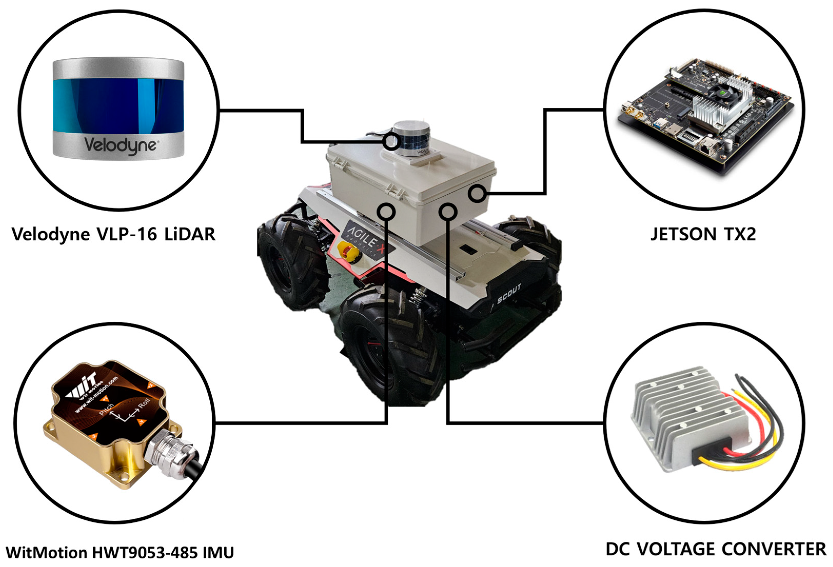
The mobile platform was employed in both baseline and orchard field experiments due to its robust capability to navigate complex, unstructured, and uneven terrain typical of agricultural environments. Featuring independent four-wheel drive, a durable chassis, and full compatibility with the ROS framework, the platform provided a stable and adaptable foundation for evaluating autonomous navigation performance under realistic outdoor conditions. To support perception, localization, and onboard computation, four primary hardware components were integrated into the system: a WHT9053-485 IMU (Witmotion Shenzhen Co., Ltd., Shenzhen, China), a Jetson TX2 embedded computing module (NVIDIA Corporation, Santa Clara, CA, USA), and two DC–DC converters (24 V to 19 V and 24 V to 12 V; EKYLIN, Shenzhen Dekelan Technology Co., Ltd., Shenzhen, China). The LiDAR sensor was mounted centrally at a height of 0.45 m above the ground to provide 360° horizontal scanning for environmental mapping and obstacle detection. During the orchard experiments, the IMU was installed within the chassis at a height of 0.25 m to provide orientation, angular velocity, and linear acceleration data, enabling real-time tilt compensation and improved pose estimation in uneven terrain. In contrast, the IMU was deliberately excluded from the baseline experiments, which were conducted on flat, open ground, to assess whether LiDAR–IMU fusion offers improved stability compared to using LiDAR alone. The Jetson TX2 functioned as the central processing unit, executing SLAM, localization, and path planning algorithms within the ROS framework. Two voltage converters ensured a stable power supply to both the Jetson TX2 and its peripheral devices, facilitating continuous operation under field conditions. This hardware configuration was maintained consistently across all trials to ensure experimental reproducibility and enable direct comparison between the baseline and sensor-fusion-enhanced systems. Figure 3 illustrates the integrated hardware setup, including sensor placement and computational modules.

2.2.2. Electrical Wiring and Power Distribution

To ensure stable operation in outdoor environments, a structured electrical and communication system was implemented on the mobile platform. In both the baseline and orchard experiments, a 24 V DC internal power supply served as the primary power source. Two DC–DC converters were employed to provide regulated outputs of 12 V and 19 V: the 12 V line powered the LiDAR sensor, while the 19 V line supplied the Jetson TX2 embedded computer. During the orchard experiments, the IMU was connected to the Jetson TX2 through a single USB cable, enabling both power delivery and data transmission while minimizing wiring complexity and electrical noise. Device communication was handled through dedicated interfaces: LiDAR data were transmitted via a LAN connection, vehicle control signals were routed through a CAN-to-USB converter, and an external HD display was connected via HDMI for real-time monitoring and debugging. All wiring and connectors were housed in weather-resistant enclosures to protect against dust, moisture, and vibration. This robust configuration ensured reliable and consistent system performance during field operations. Figure 4 illustrates the overall power distribution and communication architecture. Under representative workloads—including SLAM, global planning, and local planning—the Jetson TX2 consumed approximately 15–20 W without experiencing sustained thermal throttling. With the installed battery, the system supported continuous operation for 2–3 h, while extended missions required the integration of an auxiliary power pack.

2.3. LiDAR–IMU Sensor Calibration

2.3.1. Frame Alignment and Data Filtering

Reliable fusion of LiDAR and IMU data requires precise alignment of their coordinate frames. This was achieved using the ROS transformation library, which explicitly defined the spatial relationships between the base frame (base_link), the IMU frame (imu_link), and the LiDAR frame (velodyne). Maintaining consistent spatial alignment across all sensors was critical for accurate environmental perception and motion estimation. After alignment, raw IMU data—particularly roll and pitch—were filtered to reduce sensor noise and long-term drift. A Kalman filter was applied to smooth the IMU’s angular outputs, yielding stable orientation estimates essential for downstream tasks such as tilt compensation. The measurement noise covariance R was initialized from the variance of at least 60 s of stationary IMU data, while the process noise covariance Q was derived from the residual variance of bias estimates during low-speed straight-line driving. The Q/R ratio was subsequently fine-tuned to ensure that the per-frame Standard Deviation (SD) of roll and pitch estimates converged consistently across cross-validation runs.

2.3.2. Real-Time Tilt Compensation

To preserve the horizontal integrity of the LiDAR point cloud on sloped or uneven terrain, real-time tilt correction was applied using the filtered roll and pitch angles. Terrain-induced tilts can distort LiDAR scans, reducing the accuracy of mapping and navigation. To address this, tilt compensation was implemented through two sequential rotation matrices. The first correction addressed pitch, using the pitch rotation matrix defined in Equation (1):

$$R_{pitch}=\left[\begin{array}{ccc}\cos \left(p\right)& 0& \sin \left(p\right)\\ 0& 1& 0\\ -\sin \left(p\right)& 0& -\cos \left(p\right)\end{array}\right]$$

(1)

Next, roll angle correction was applied using a roll rotation matrix, as defined in Equation (2):

$$R_{roll}=\left[\begin{array}{ccc}1& 0& 0\\ 0& \cos \left(r\right)& -\sin \left(r\right)\\ 0& \sin \left(r\right)& \cos \left(r\right)\end{array}\right]$$

(2)

where $p$ and $r$ represent the filtered pitch and roll angles, respectively. Each LiDAR point $[x,y,z]$ sequentially transformed using the pitch and roll rotation matrices, resulting in corrected coordinates $[x^{\prime },y^{\prime },z^{\prime }]$, as shown in Equation (3):

$$\left[\begin{array}{c}{x}^{\prime }\\ y^{\prime }\\ z^{\prime }\end{array}\right]=R_{pitch}·R_{roll}·\left[\begin{array}{c}x\\ y\\ z\end{array}\right]$$

(3)

By applying these transformations in real time, the system continuously corrected tilt-induced distortions, thereby preserving the horizontal alignment of the point cloud. This significantly improved the reliability of the environmental map and enhanced the accuracy of both localization and path planning.

2.3.3. LiDAR–IMU Calibration Workflow

The calibration procedure followed a structured sequence comprising IMU data acquisition, noise filtering, frame alignment, and tilt compensation. IMU orientation data were first collected continuously and stabilized with a Kalman filter to suppress sensor noise and drift. Coordinate transformations were then configured to align the robot’s base, IMU, and LiDAR frames within a unified reference system. Using the filtered roll and pitch values, tilt correction was applied through sequential rotation matrices to generate a level LiDAR point cloud independent of terrain slope. This correction minimized perception errors caused by platform inclination and preserved the horizontal integrity of the LiDAR data. The corrected point cloud was subsequently integrated into the mapping and localization modules, supporting accurate SLAM and navigation. The calibration approach was validated through field trials in orchard environments characterized by uneven ground, slopes, and obstacles. By directly linking each step to the filtering, calibration, and mapping procedures in Figure 5, the flow diagram now serves as a clear visual reference that integrates seamlessly with the overall experimental design.

2.4. Path Planning and Path Tracking

2.4.1. Path Planning with A*, RRT, and Improved RRT

Path planning is essential for autonomous navigation, enabling the robot to compute efficient routes from its current position to a designated target while avoiding obstacles. This study proposes an Improved Rapidly-Exploring Random Tree (Improved RRT) algorithm to overcome key limitations of the conventional RRT, which often generate inefficient and suboptimal paths. To assess its performance, A* and standard RRT algorithms were implemented as a comparative baseline. Although RRT is widely adopted for high-dimensional motion planning due to its exploratory capabilities, it typically exhibits random, inefficient growth patterns that often result in unnecessary detours. These irregular paths not only increase travel distance but also complicate tracking by necessitating frequent heading corrections. Moreover, the computational burden of traditional RRT increases substantially in large-scale or cluttered environments, as a high number of sampled nodes is required to reach the target.

Improved RRT addresses these challenges by incorporating a direct-path prioritization mechanism. During tree expansion, the algorithm evaluates whether a newly sampled node ${(x}_{new})$ can be directly connected to the goal node ${(x}_{goal})$ based on a set of predefined criteria. The first condition assesses whether the Euclidean distance between the nodes falls within a specified threshold, as defined in Equation (4):

$$d(x_{new},x_{goal})\le ϵ$$

(4)

where $d(x_{new},x_{goal})$ denotes the Euclidean distance between the newly sampled node and the goal, and $ϵ$ specifies the maximum allowable distance for a direct connection.

The second condition examines the straightness of the trajectory by analyzing the angular deviation between consecutive segments. For the segment formed by $x_{prev}$, $x_{new}$, and $x_{goal}$, the condition is satisfied if the deviation and $\theta$ meet the criterion defined in Equation (5):

$$\theta ={\cos }^{-1}\left({\displaystyle \frac{{(x}_{new}-x_{prev})·{(x}_{goal}-x_{new})}{‖x_{new}-x_{prev}‖·‖{(x}_{goal}-x_{new}‖}}\right)\le {\theta }_{max}$$

(5)

If both the distance and smoothness conditions are satisfied, the tree extends directly toward the goal, thereby reducing unnecessary waypoints and eliminating redundant path segments. By prioritizing feasible direct connections, the algorithm minimizes detours and enhances computational efficiency. The distance threshold (ε) and smoothness limit (${\theta }_{max}$) were optimized through grid search on a simulation validation set, yielding ε = 2.0 m in simulation and 1.2 m in field experiments, with ${\theta }_{max}$ = 15°. These settings encouraged goal-directed connections while preventing zig-zagging trajectories. Collision avoidance was enforced using a robot inflation radius of 0.35 m combined with ray-casting on the occupancy map.

For benchmarking, the Improved RRT was compared against both the traditional RRT and A* algorithms. The A* algorithm served as a baseline due to its ability to generate optimal paths via heuristic-based search; however, its exhaustive search strategy incurs high computational costs, limiting its practicality in large-scale or dynamic environments. In contrast, traditional RRT enables rapid path generation but often produces irregular and suboptimal trajectories, thereby requiring frequent corrections during execution.

The Improved RRT achieves a strong balance between computational efficiency and path quality, significantly reducing unnecessary deviations while maintaining real-time performance. These enhancements are particularly beneficial for autonomous navigation in agricultural settings, where energy efficiency and operational reliability are critical.

2.4.2. Path Tracking Algorithms

Path tracking ensures that the robot accurately follows a pre-planned trajectory while responding to real-time environmental changes. In this study, two path-tracking algorithms—the DWA and Pure Pursuit—were selected based on the experimental context and path characteristics.

The DWA was employed in simulation and baseline experiments where dynamic obstacle avoidance was required. This local trajectory optimization method generates real-time velocity commands by accounting for the robot’s kinematic constraints, proximity to obstacles, and alignment with the planned path. At each time step, DWA evaluates a set of velocity candidates by simulating their resulting trajectories and assigning costs based on obstacle clearance, trajectory deviation, and smoothness. The velocity pair with the lowest total cost is then selected for execution. Integrated within the ROS move_base framework, DWA proved particularly effective in test environments featuring dynamic obstacles, such as speed bumps and artificial trees. Its ability to dynamically optimize movement, rather than strictly follow a predefined path, enhanced its robustness in unpredictable conditions.

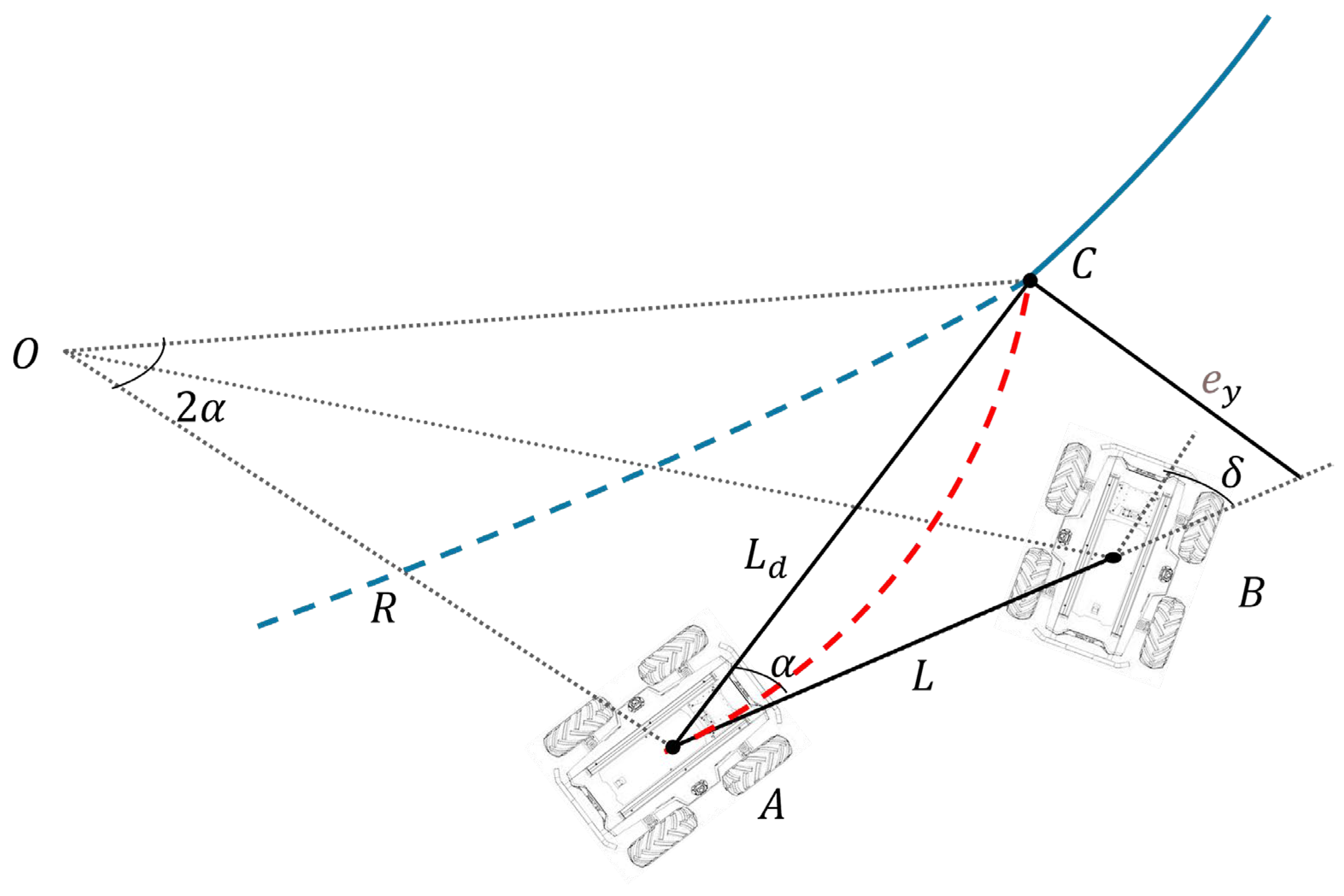
In contrast, the Pure Pursuit algorithm was applied during the orchard experiments, where the primary objective was to achieve smooth and stable navigation along structured paths. This algorithm computes the appropriate steering angle by identifying a look-ahead point at a fixed distance along the trajectory. The robot continuously adjusts its heading to minimize the curvature between its current position and the look-ahead point, enabling smooth and consistent path tracking.

The trajectory curvature $a$, which governs the robot’s turning radius, is calculated using Equation (6):

$$\alpha ={\displaystyle \frac{2·e_y}{L_d^2}}$$

(6)

where $e_y$ denotes the lateral error, and $L_d$ represents the look-ahead distance. This curvature value guides the robot’s heading adjustment to maintain alignment with the desired trajectory.

Once the curvature is determined, the corresponding steering angle $\beta$ is computed using Equation (7):

$$\beta ={\tan }^{-1}\left({\displaystyle \frac{2a·e_y}{L_d^2}}\right)$$

(7)

where $a$ denotes half the robot’s wheelbase. By continuously updating $e_y$ and recalculating $\beta$, the algorithm enables real-time adjustments to maintain stable and accurate trajectory tracking.

The Pure Pursuit algorithm proved particularly effective in structured orchard environments, where the absence of dynamic obstacles allowed for smooth and uninterrupted navigation. It minimized abrupt deviations and ensured consistent movement through narrow, curved orchard rows. As shown in Figure 6, the robot continuously adjusted its heading toward a dynamically updated look-ahead point, thereby reducing trajectory oscillations and enhancing path stability.

Compared to DWA, which excels in dynamically changing environments by reactively adjusting velocities, Pure Pursuit offered superior trajectory smoothness and tracking precision in static environments. A comparative analysis of both methods highlights their environmental suitability: DWA was optimal for environments with frequent, unpredictable obstacles, as demonstrated in the baseline tests, while Pure Pursuit provided enhanced accuracy and stability in structured settings such as orchards.

2.5. Mapping and Localization

2.5.1. Point Cloud-to-Laser Scan Conversion

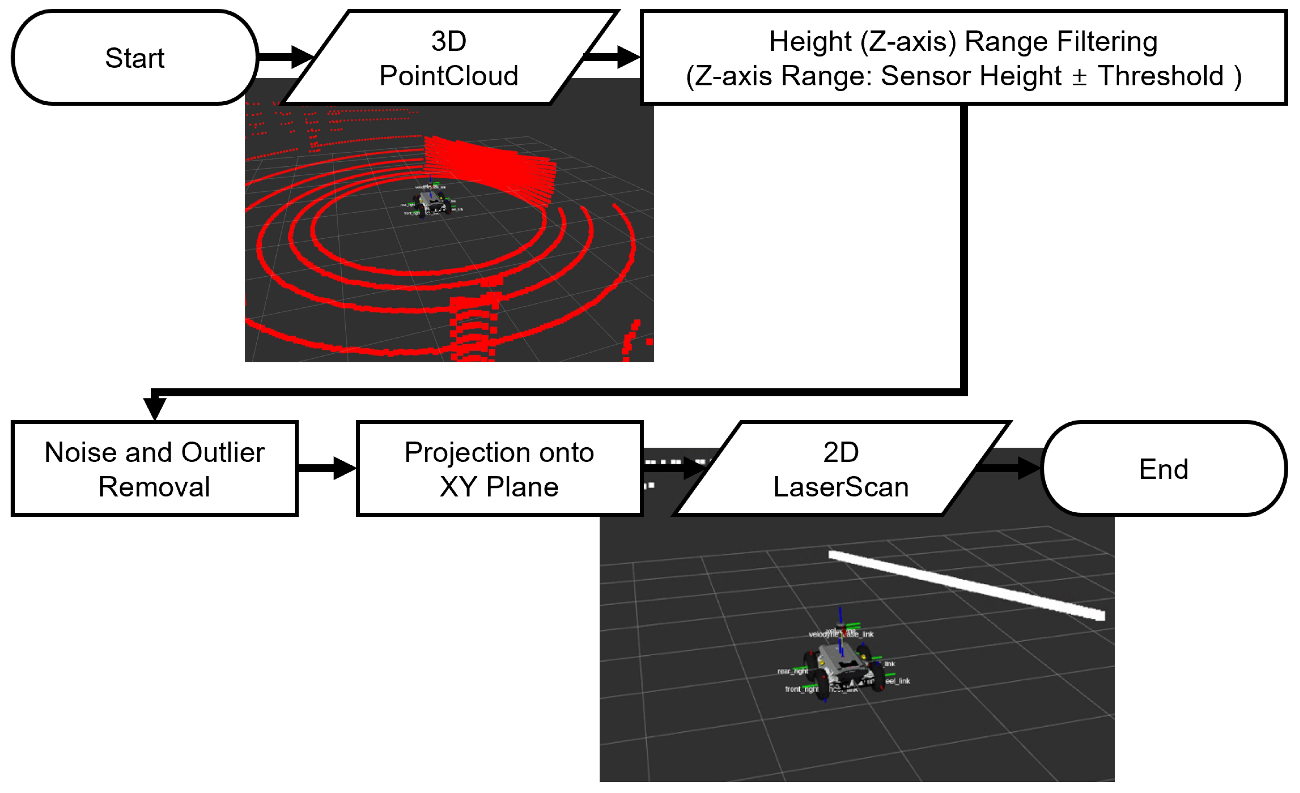
Ensuring high accuracy and real-time responsiveness was a primary objective of the system. The LiDAR sensor used in this study generated dense 3D point cloud data with high spatial resolution. However, directly processing this data for SLAM and navigation imposed significant computational demands. To address this issue, the pointcloud_to_laserscan package (version 1.4.1, Open Source Robotics Foundation, Mountain View, CA, USA) in ROS was utilized to convert 3D point clouds into a 2D laser scan format. During this conversion, only points within a specified height range (0.5–1.5 m above ground level) were retained, effectively filtering out ground reflections and overhead canopy noise. This selective filtering preserved critical environmental features within the robot’s operational zone while eliminating irrelevant data.

The resulting 2D scan data were published to the /scan topic, enabling seamless integration with downstream modules such as SLAM and local planners. To further improve scan quality, preprocessing techniques—including voxel grid filtering and statistical outlier removal—were employed. These methods effectively reduced noise and point redundancy, thereby enhancing the reliability of subsequent mapping and localization tasks. The effectiveness of this strategy was validated by comparing raw 3D point clouds with their converted 2D scan counterparts. The 2D scans retained essential structural information while significantly reducing computational load, thus supporting real-time SLAM and path planning in both structured and unstructured environments. Figure 7 illustrates the complete data transformation pipeline, from 3D point cloud acquisition to 2D laser scan generation.

2.5.2. SLAM with Gmapping

SLAM is essential for autonomous navigation in unknown environments. In this study, 2D SLAM was implemented using the slam_gmapping package (version 1.4.2, OpenSLAM.org, Freiburg, Germany) in ROS, which utilized the previously converted 2D laser scans from the LiDAR sensor. During the experiments, the robot was manually driven through both a controlled testbed and an actual orchard environment. The slam_gmapping node processed the incoming scan data in real time to generate an occupancy grid map. Key parameters, such as map resolution, update frequency, and scan-matching thresholds, were carefully tuned to enhance mapping accuracy and consistency. The generated map was continuously updated and published to the /map topic, while a static version was saved using the map_server node (version 1.16.7, Open Source Robotics Foundation, Mountain View, CA, USA) for subsequent localization tasks. Figure 8 illustrates the interaction between slam_gmapping and map_server within the SLAM workflow.

To ensure repeatability and robustness, multiple mapping trials were conducted. Special attention was given to high-density areas, such as orchard tree rows, where overlapping features can compromise scan clarity. To mitigate this issue, adaptive filtering and fine-grained scan matching techniques were applied, enhancing map fidelity in cluttered environments. The final maps were exported in PGM and YAML formats and served as the foundation for localization using the Adaptive Monte Carlo Localization (AMCL) algorithm. The quality of these maps was essential for maintaining reliable and accurate localization in both static and dynamically changing environments.

2.6. Integrated Navigation System

2.6.1. Global Planner Integration

To achieve precise and stable autonomous navigation, all core modules—including mapping, localization, global path planning, and local control—were integrated within the ROS move_base framework. Global trajectories were generated using three planning algorithms: A*, RRT, and the proposed Improved RRT. These planners computed optimal trajectories from the robot’s current pose, estimated by the AMCL module, to user-defined goal points. Among them, the Improved RRT algorithm demonstrated notable advantages in complex environments. Applying both distance and angular constraints during node sampling enabled direct path extensions toward the goal, effectively minimizing detours and redundant segments. This capability was particularly valuable in orchard settings, where the irregular arrangement of trees often poses challenges to traditional sampling-based methods. Once the global path was generated, it was passed to the local planner for execution. The DWA was selected for baseline experiments due to its adaptability to dynamic obstacles, whereas Pure Pursuit was used in orchard trials to ensure smooth and stable tracking along curved, structured paths.

2.6.2. Overall System Architecture

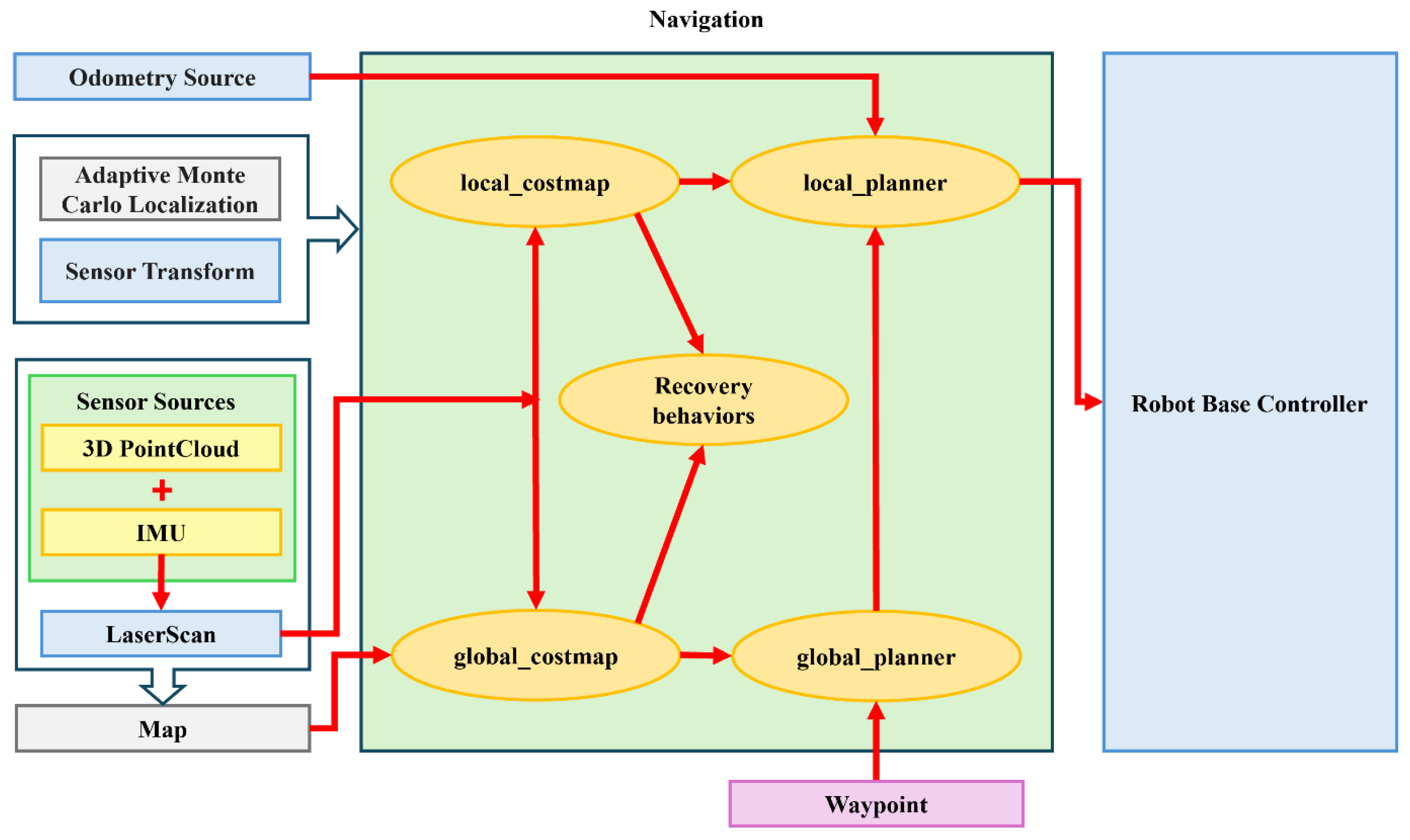
The navigation system was developed using a modular, ROS-based architecture, with each function—sensor processing, state estimation, mapping, planning, and control—implemented as an independent node. This modularity ensured clear data flow, facilitated debugging, and supported flexible component upgrades. Sensor data were continuously published by dedicated driver nodes. The Velodyne LiDAR generated raw point clouds, which were subsequently filtered and converted into 2D laser scans. Simultaneously, the IMU provided orientation data, which were filtered using a Kalman filter to reduce noise and enhance pose estimation. Localization was handled by the robot_localization package (version 2.6.11, Open Source Robotics Foundation, Mountain View, CA, USA), which fused odometry and IMU data through an Extended Kalman Filter (EKF) algorithm to maintain accurate tracking on uneven terrain. Coordinate transformations among the robot’s base frame (base_link), LiDAR (velodyne), and IMU (imu_link) were maintained using ROS’s transform tree to ensure spatial consistency.

During the mapping phase, the slam_gmapping node generated 2D occupancy grid maps, which were saved using map_server and later utilized by the AMCL module for localization. AMCL employed a particle filter to match real-time laser scans with the static map and odometry data, continuously refining the robot’s pose estimate. Global path planning was performed using the Improved RRT algorithm within the move_base node. The computed path was published to the /move_base/GlobalPlanner/plan topic and then tracked by the selected local planner, which generated velocity commands published to the/cmd_vel topic for execution. To ensure operational safety, an additional monitoring layer continuously checked for nearby obstacles. If any object was detected within a 0.25-m radius, the system automatically issued a stop command to prevent collisions. The complete system architecture—including sensor data flow, planning hierarchy, and control mechanisms—is illustrated in Figure 9, which outlines the integrated LiDAR–IMU fusion-based navigation framework.

2.7. Baseline Experiment Design

To assess the core performance of the autonomous navigation system, a baseline experiment was conducted on 1 September 2024, in a structured outdoor testbed designed to replicate orchard-like conditions. The primary objectives were to assess mapping accuracy, localization stability, and the system’s response to terrain irregularities. The test environment featured six artificial trees, each measuring 1.2 m in height, arranged in two parallel rows to simulate orchard lanes. Additionally, two speed bumps were placed along the navigation path to introduce pitch disturbances and emulate the effects of uneven terrain. For this experiment, the robot platform was equipped solely with a Velodyne VLP-16 LiDAR sensor—no IMU was used—to isolate and evaluate the performance of LiDAR-only navigation.

Three global path planning algorithms—A*, RRT, and the proposed Improved RRT—were implemented to generate navigation paths. For local path tracking, the DWA was employed due to its effectiveness in real-time velocity selection and obstacle avoidance in constrained environments. This controlled setup served as a baseline for analyzing the system’s performance without inertial feedback. Although the LiDAR-based system achieved basic navigation, the lack of IMU input limited its ability to compensate for terrain-induced roll and pitch, particularly during traversal over speed bumps. The experimental layout is illustrated in Figure 10. Figure 10a presents the testbed configuration and the locations of the speed bumps, while Figure 10b depicts the designated driving directions used during the trials.

2.8. Orchard Experiment Design

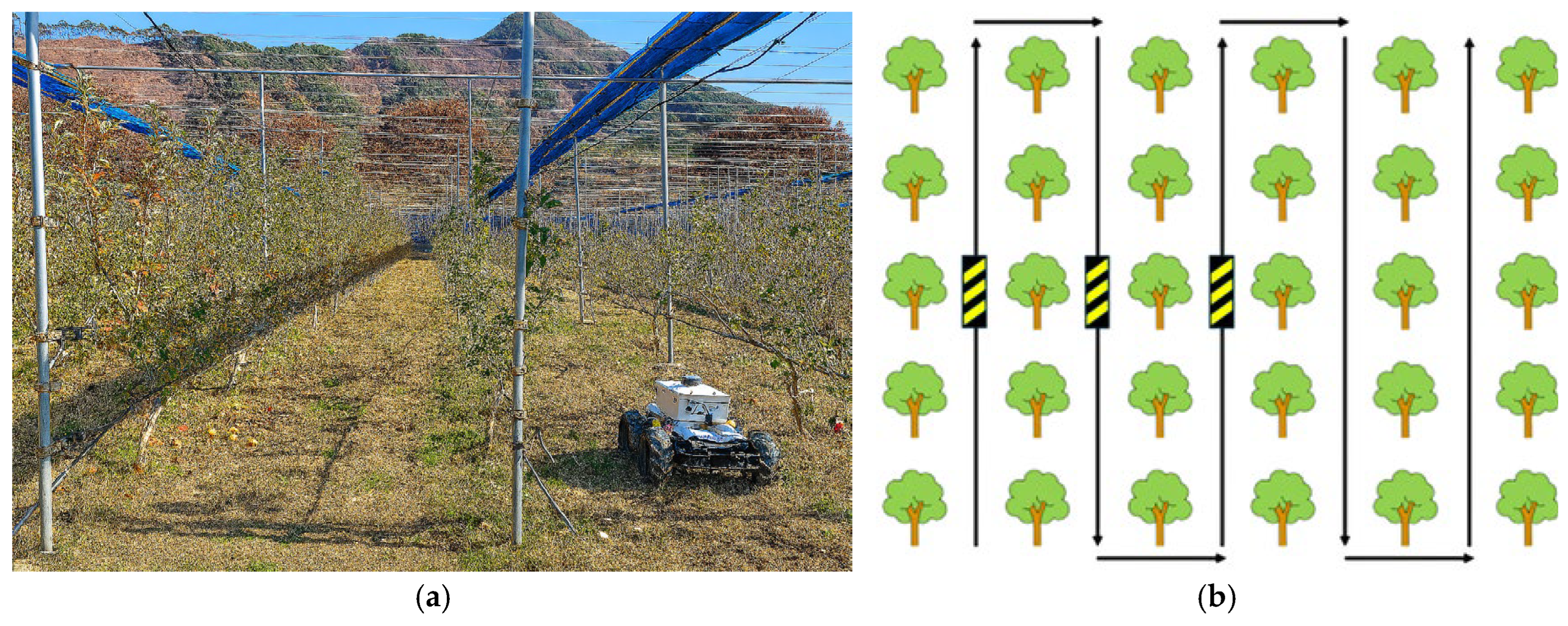
To evaluate the navigation system under realistic and challenging field conditions, experiments were conducted from 7 to 18 October 2024, in a commercial apple orchard managed by the Gangwon-do Agricultural Research and Extension Services. The orchard featured tree rows spaced 2.5 m apart, with individual trees positioned approximately 1 m apart. The environment presented natural complexities, such as exposed roots, uneven slopes, and low-hanging branches—conditions typical of real-world agricultural settings. In this experiment, the mobile platform was equipped with both LiDAR and IMU sensors, enabling real-time LiDAR–IMU fusion for enhanced localization and mapping accuracy. For local path tracking, the Pure Pursuit algorithm was employed instead of DWA. While DWA excels in dynamic environments with its rapid obstacle avoidance capabilities, its reactive nature often results in oscillatory motion. In contrast, Pure Pursuit provided smoother and more stable trajectory tracking, making it more suitable for the orchard’s static and structured layout.

The same global path planning algorithms—A*, RRT, and the proposed Improved RRT—were tested using identical start and goal positions. System performance was evaluated using key metrics, such as root mean square error (RMSE) between planned and actual trajectories, time to reach the target, and obstacle avoidance success rate. Notably, GPS was not used in this experiment; all localization was achieved through LiDAR–IMU sensor fusion. This field trial demonstrated the system’s robustness in complex outdoor environments, effectively addressing limitations identified in the baseline tests and validating its practical applicability to autonomous navigation in agricultural operations. The layout of the orchard experiment is illustrated in Figure 11. Figure 11a shows the test site and obstacle locations, while Figure 11b depicts the driving directions used during the trials.

3. Results

3.1. Simulation Experiment

Simulation experiments were conducted with three repetitions per condition (n = 3). Unless otherwise specified, all performance metrics are reported as mean ± SD. Metrics with negligible variability or deterministic outcomes are presented as single values, while the “±” notation in tables and figures indicates SD. To evaluate the effectiveness of different path planning strategies in orchard environments, autonomous navigation experiments were conducted within a virtual simulation platform. Four algorithms—A*, RRT, Improved A*, and Improved RRT—were compared using key performance metrics: time to destination, total driving distance, RMSE of the trajectory, and yaw rate stability. Additionally, SLAM performance was assessed using the Gmapping package to evaluate environmental reconstruction accuracy. Figure 12a illustrates the simulated orchard environment constructed in Gazebo, where tree rows and pathways were arranged to mimic realistic field conditions. The occupancy grid map generated through Gmapping-based SLAM is presented in Figure 12b. The Gmapping-based SLAM accurately reconstructed the structural layout, including tree rows and pathways, and reliably captured the planned navigation trajectories. To improve map clarity and minimize noise, the LiDAR detection range was limited to 3 m, resulting in dense, high-resolution maps suitable for precise navigation.

The driving trajectories generated by each algorithm are presented in Figure 13. Among them, Improved RRT (Figure 13d) produced the most stable and linear path, characterized by smooth transitions and precise adherence to the planned trajectory. In contrast, the A* algorithm (Figure 13a) generated angular paths with sharp turns, resulting in reduced stability. The RRT algorithm (Figure 13b) exhibited irregular movement and frequent deviations from the intended path, leading to low path fidelity. The Improved A* algorithm (Figure 13c) demonstrated greater smoothness than A*, although minor instability remained in straight sections.

The quantitative results are summarized in

Table 1. Results of trajectory accuracy and stability for four path planning algorithms in a simulated orchard environment.

Algorithm	A*	RRT	Improved A*	Improved RRT
Time to Destination (s)	88.318 ± 0.521	92.634 ± 0.613	89.762 ± 0.476	90.814 ± 0.501
Driving distance (m)	64.341 ± 0.215	66.561 ± 0.308	57.480 ± 0.182	56.826 ± 0.197
RMSE (cm)	3.600 ± 0.200	5.400 ± 0.300	2.900 ± 0.200	2.300 ± 0.100
Maximum Yaw Rate (rad·s−1)	1.037 ± 0.024	0.950 ± 0.018	0.907 ± 0.015	0.905 ± 0.012
Average Yaw Rate (rad·s−1)	0.305 ± 0.013	0.376 ± 0.012	0.352 ± 0.011	0.349 ± 0.009

. Among the algorithms, Improved RRT achieved the shortest and most accurate path, with a total driving distance of 56.826 m and an RMSE of 2.362 cm. In contrast, RRT generated the longest path (66.561 m) and the highest RMSE (5.423 cm), indicating inefficient and unstable routing. The A* algorithm produced a path length of 64.341 m with an RMSE of 3.634 cm, while the Improved A* recorded 57.480 m and 2.927 cm, respectively. Regarding travel time, A* achieved the shortest time to destination (88.318 s), followed by Improved A* (89.762 s) and Improved RRT (90.814 s). RRT recorded the longest travel time (92.634 s), primarily due to its stochastic sampling behavior, which resulted in unnecessary detours.

Yaw rate analysis further highlighted the advantages of the Improved RRT. It achieved the lowest maximum yaw rate (1.037 rad·s⁻¹) and the lowest average yaw rate (0.352 rad·s⁻¹), indicating smooth heading transitions and minimal oscillations. In contrast, RRT exhibited the highest yaw instability, with a maximum yaw rate of 0.950 rad·s⁻¹ and an average of 0.376 rad·s⁻¹. These results indicate that combining Gmapping-based SLAM with the globally optimized Improved RRT algorithm enables accurate environmental mapping, efficient path planning, and stable motion control. Overall, the proposed system shows strong potential for real-world deployment in complex orchard environments.

3.2. Baseline Experiment

To assess the real-world navigation performance of different path planning algorithms in a structured outdoor setting, baseline experiments were conducted using A*, RRT, and the proposed Improved RRT. Key performance metrics included total path length, RMSE, time to destination, and yaw rate stability. Figure 14 presents the driving trajectories generated during outdoor testing for each algorithm: (a) A*, (b) RRT, and (c) Improved RRT. Baseline results were obtained from three repetitions per condition (n = 3). Unless otherwise specified, all reported values represent mean ± SD.

The A* algorithm generated structurally optimal paths using grid-based heuristics; however, its rigid turning behavior and angular transitions resulted in relatively long driving distances. The RRT algorithm, while effective in rapidly identifying feasible routes through random sampling, often produced irregular trajectories with sharp turns and unnecessary detours. In contrast, the Improved RRT algorithm prioritized straight-line connections and minimized redundant nodes, resulting in smoother, more natural trajectories that closely adhered to the intended waypoints.

The quantitative results are summarized in

Table 2. Quantitative performance comparison of path planning algorithms in baseline experiments.

Algorithm	Path	RMSE (cm)	Average RMSE (cm)	Time Consumption (s)
A*	Line 1	2.3	3.4 ± 0.3	63.078
	Line 2	4.3
	Line 3	3.8
RRT	Line 1	3.3	3.7 ± 0.4	69.265
	Line 2	3.6
	Line 3	4.2
Improved RRT	Line 1	2.1	2.2 ± 0.2	76.428
	Line 1	2.4
	Line 2	2.2

. The Improved RRT achieved the lowest average RMSE of 2.2 ± 0.2 cm, demonstrating high efficiency and precision. In comparison, the A* and RRT recorded average RMSE values of 3.4 ± 0.3 cm and 3.6 ± 0.4 cm, respectively. Although A* yielded the shortest travel time (63.078 s), its longer path and lower trajectory accuracy limited overall performance. The Improved RRT provided superior accuracy and smoother motion quality, with only a modest increase in computation time (76.428 s). By contrast, RRT completed the route in 69.265 s but produced less refined and less consistent trajectories than the Improved RRT.

Motion stability was further assessed through yaw rate analysis, with the results presented in Figure 15: (a) A*, (b) RRT, and (c) Improved RRT. Among the three algorithms, the Improved RRT demonstrated the most stable navigation, with an average yaw rate of 0.745 rad·s⁻¹, indicating smooth heading transitions. RRT showed the highest instability, characterized by large oscillations and a peak yaw rate of 1.417 rad·s⁻¹. The A* algorithm exhibited moderate stability, with fewer oscillations than RRT but more than Improved RRT. Overall, these findings confirm that the Improved RRT achieves an effective balance between trajectory efficiency, accuracy, and stability, consistently outperforming both A* and RRT across all evaluation criteria.

3.3. Orchard Experiment

Unlike the controlled baseline trials, the orchard experiments were constrained by practical factors such as limited field access, battery endurance, and uncontrollable environmental variability, which made identical repetitions impractical. Consequently, these trials were primarily intended to validate the feasibility and robustness of the system under real-world conditions rather than to establish statistical repeatability. Statistical variability has already been characterized in the baseline experiments, while future work will expand orchard trials to include larger-scale repetitions across seasons and terrains.

To assess the performance of the proposed autonomous navigation system under real-world, unstructured conditions, field experiments were conducted in a commercial apple orchard. The evaluation focused on four key aspects: mapping accuracy, path planning performance, trajectory consistency, and motion stability. Special attention was given to the role of LiDAR–IMU fusion in enhancing the system’s robustness on sloped and uneven terrain—conditions commonly encountered in agricultural environments.

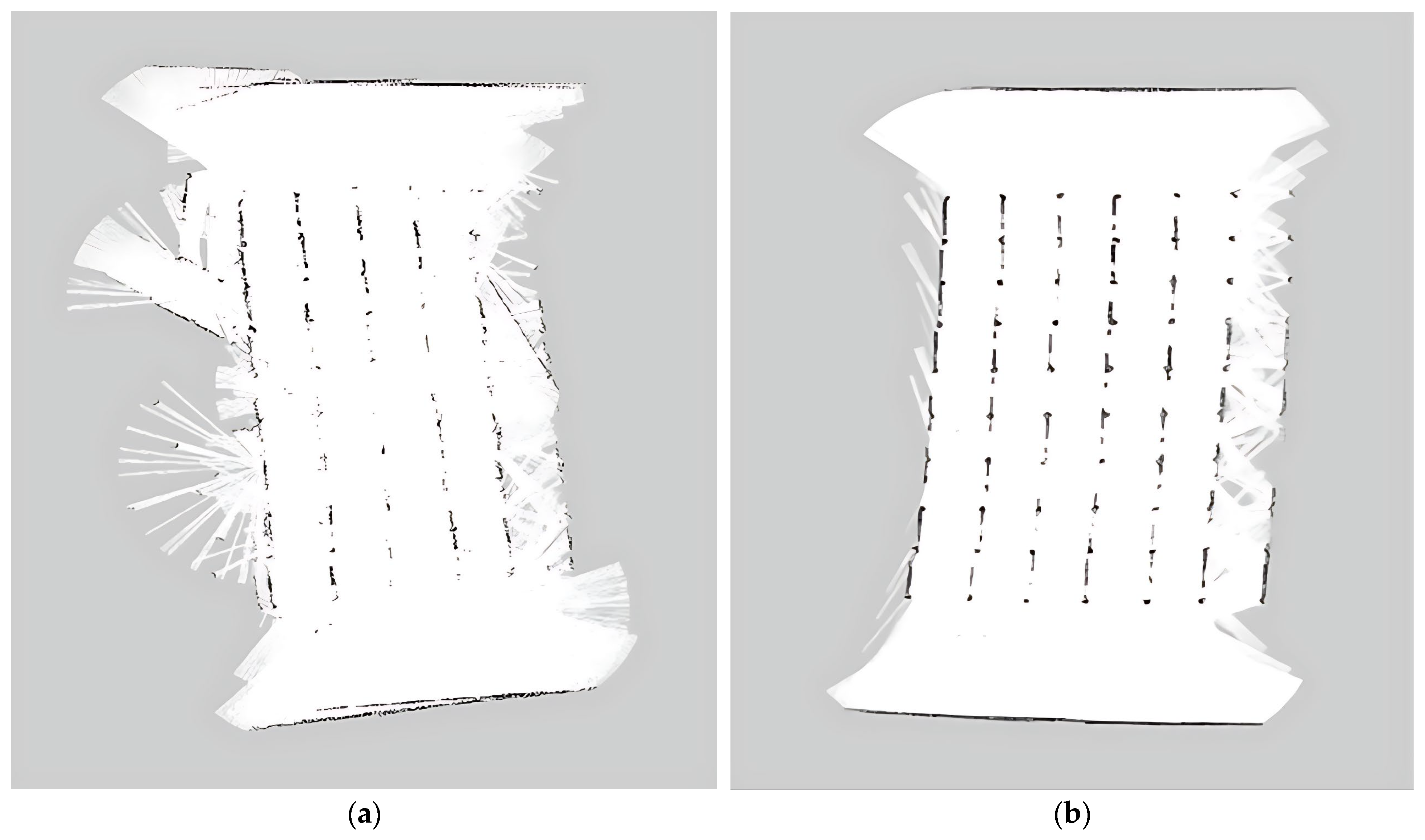
Figure 16 compares occupancy grid maps generated under two different sensor configurations. Figure 16a shows the map produced using LiDAR alone, which displays noticeable distortion and noise resulting from uncorrected pitch and roll variations caused by the uneven terrain. In contrast, Figure 16b presents the map generated through LiDAR–IMU fusion, where real-time orientation compensation significantly improved structural clarity and map fidelity. These results highlight the critical role of IMU integration in achieving accurate and stable environmental mapping under complex field conditions. By mitigating terrain-induced motion artifacts, LiDAR–IMU fusion enhances both mapping quality and downstream localization performance, ultimately contributing to more reliable autonomous navigation in agricultural applications.

The path planning results for each algorithm are presented in Figure 17. As shown in Figure 17a, A* generated geometrically constrained yet angular trajectories, often characterized by sharp turns and abrupt directional changes. In contrast, Figure 17b reveals that RRT produced more flexible but highly irregular paths, with noticeable variation in quality across different trials. Figure 17c illustrates that Improved RRT achieved a better balance between structural rigidity and path flexibility, resulting in smoother and more continuous trajectories that closely followed the natural curvature of orchard rows while avoiding unnecessary detours.

To quantitatively assess tracking accuracy, RMSE was calculated for four straight-line segments, each starting from a different point within the orchard but sharing consistent environmental features, such as tree row spacing. The results are summarized in

Table 3. Quantitative performance comparison of path planning algorithms from the orchard experiments.

Line Segment	A* RMSE (m)	RRT RMSE (m)	Improved RRT RMSE (m)
Line 1	0.914	0.962	0.959
Line 2	0.896	0.817	0.834
Line 3	0.937	0.107	0.978
Line 4	0.801	0.702	0.790
Average RMSE	0.894	0.887	0.890

. In Line 1, A* achieved the lowest RMSE (0.914 m), slightly outperforming RRT (0.962 m) and Improved RRT (0.959 m). In Line 2, RRT recorded the best performance (0.817 m), followed by Improved RRT (0.834 m) and A* (0.896 m). For Line 3, RRT again achieved the lowest RMSE (0.107 m), likely due to coincidental alignment with the optimal trajectory, whereas A* and Improved RRT had higher errors of 0.937 m and 0.978 m, respectively. In Line 4, Improved RRT delivered the best performance with an RMSE of 0.790 m, indicating superior adaptability in that segment. When averaged across all four segments, A* produced an RMSE of 0.894 m, RRT 0.887 m, and Improved RRT 0.890 m. Although the average RMSE values were close, A* and RRT exhibited greater variability across trials. In contrast, Improved RRT maintained more consistent performance, underscoring its potential for reliable and repeatable deployment in real-world autonomous navigation applications.

Deviation responses were evaluated along a straight orchard segment embedded with artificial speed bumps to simulate terrain-induced disturbances. Rather than presenting numerical data in tabular form, the deviation behavior for each algorithm is visualized in Figure 18, which plots the robot’s X-position, reference waypoints, and calculated deviations across 30 checkpoints. As shown in Figure 18a, A* exhibited a gradual increase in deviation around the midpoint, peaking at approximately 1.2 m. Although the deviation was moderate, the system’s recovery was slow, indicating limited resilience to pitch-induced disturbances. In contrast, RRT (Figure 18b) showed the highest deviation amplitudes, with multiple peaks exceeding 2.0 m and unstable tracking throughout the segment. However, Improved RRT (Figure 18c) maintained tightly bounded deviations and demonstrated quick recovery after encountering bumps, with most deviations remaining within 1.0 m. This indicates stronger path fidelity and robustness on uneven terrain.

The quantitative results are summarized in

Table 4. Driving RMSE results for different path planning algorithms from orchard experiments.

Algorithm	Straight with Bumps (RMSE; cm)	Rotation (RMSE; cm)
A*	8.900	27.600
RRT	14.300	27.500
Improved RRT	8.500	24.100

. For straight-line segments with bumps, Improved RRT achieved the lowest RMSE (8.52 cm), followed by A* (8.95 cm) and RRT (14.35 cm). On rotational segments, Improved RRT again outperformed the other algorithms, recording an RMSE of 24.13 cm compared to 27.68 cm for A* and 27.52 cm for RRT. These results further highlight the Improved RRT’s superior stability and precision under dynamic field conditions commonly encountered in agricultural environments.

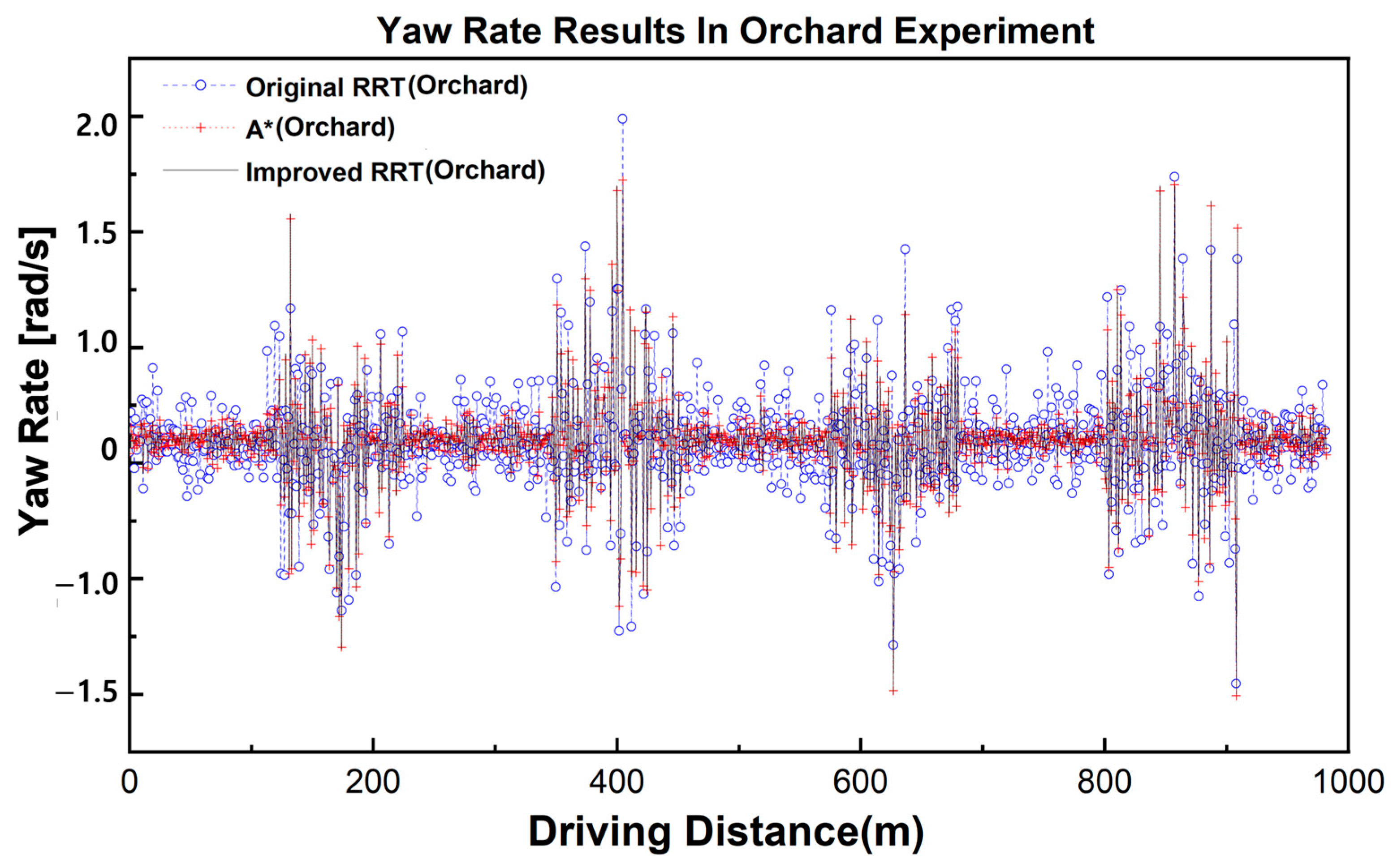
To further evaluate the rotational stability of each path planning algorithm, yaw rate data were analyzed throughout the orchard navigation trials. Figure 19 displays the yaw rate profiles plotted against cumulative driving distance, providing a comparative view of each algorithm’s rotational behavior under real-world conditions. The Y-axis represents angular velocity, while the X-axis corresponds to cumulative travel distance.

As shown in Figure 19, RRT exhibited the highest level of rotational instability, characterized by frequent sharp spikes and large fluctuations in yaw rate. This erratic behavior reflects poor heading control and abrupt turning. The A* algorithm demonstrated improved stability compared to RRT but still experienced periodic abrupt changes, particularly during direction reversals or tight turns. In contrast, Improved RRT displayed the most stable rotational performance, with smooth transitions and narrower fluctuation bands throughout the entire route. Such stability reduces mechanical stress and enhances reliability, especially in tasks requiring precise orientation changes, such as navigating between narrow orchard rows.

The quantitative results are summarized in

Table 5. Comparison of yaw rate across the three planning algorithms during the orchard experiments.

Metric (rad·s−1)	A*	RRT	Improved RRT
Mean	0.156	0.173	0.174
Std	0.378	0.357	0.355
Min	−1.665	−1.757	−1.745
Max	2.598	2.134	2.080

. Although the average yaw rates were comparable—0.156 rad·s⁻¹ for A*, 0.173 rad·s⁻¹ for RRT, and 0.174 rad·s⁻¹ for Improved RRT—SD values revealed significant differences. The Improved RRT exhibited the lowest yaw rate variability (0.355 rad·s⁻¹), followed by A* (0.357 rad·s⁻¹), while RRT showed the highest variability (0.378 rad·s⁻¹). Additionally, the Improved RRT demonstrated the narrowest range of rotational motion, with minimum and maximum yaw values spanning from −1.745 to 2.080 rad·s⁻¹. This range was more constrained than those of A* (−1.665 to 2.598 rad·s⁻¹) and RRT (−1.757 to 2.134 rad·s⁻¹), indicating a more controlled and predictable rotational behavior.

4. Discussion

Accurate localization and robust path planning remain critical challenges for autonomous navigation in unstructured orchard environments. Prior studies have often relied either on 2D LiDAR pipelines without inertial compensation or on tightly coupled multi-sensor stacks that include RTK GNSS. For example, Nazate-Burgos et al. [35] proposed a 2D SLAM framework using the Modified Hausdorff Distance and EKF, reporting an RMSE of approximately 0.84 m in orchards and vineyards. However, the absence of roll and pitch compensation allowed elevation changes and platform tilting to propagate into pose drift. In contrast, the present system fuses 3D LiDAR-derived 2D scans with IMU tilt feedback, stabilizing scan geometry on uneven terrain. Over artificial bumps, trajectory RMSE decreased to about 8.52 cm, clearly demonstrating the benefits of inertial fusion under vibration and slope. Nazate-Burgos et al. [35] similarly reported that even small elevation variations degraded SLAM accuracy by several centimeters when tilt correction was not applied. In our framework, continuous scan-angle adjustment based on IMU roll and pitch feedback effectively mitigated this effect in both baseline and orchard trials. As shown in Figure 14, the estimated path remained closely aligned with waypoints, while yaw excursions were bounded in curved segments, supporting improved mapping fidelity and trajectory stability under transient attitude changes.

On the planning side, Ye et al. [32] introduced CBQ-RRT*, achieving an average tracking error of approximately 33.4 cm in orchard trials—an improvement over standard Bi-RRT*. Nevertheless, residual sharp turns and redundant nodes persisted in dense rows. By comparison, the proposed Improved RRT prioritized straight connections, pruned redundant nodes, and incorporated yaw-aware control. As a result, tracking errors were reduced to approximately 8.52 cm on straight segments and 24.13 cm on curved paths, while yaw rate spikes were mitigated, reducing controller saturation and overshoot. These improvements stem from smoother node transitions and a planning policy that anticipates heading changes rather than merely reacting to them. Wang et al. [36] reported a lateral error of about 4.16 cm using a tightly coupled GNSS–LiDAR–IMU stack with RTK corrections. While highly accurate, such systems are vulnerable to canopy-induced GNSS signal loss and require costly infrastructure. In contrast, the proposed system operates independently of GNSS while still achieving sub-decimeter accuracy on straight paths and decimeter-level accuracy on low-speed curves, offering greater practicality in signal-denied orchard environments.

From an implementation perspective, projecting 3D LiDAR data into 2D scans preserved essential geometric information while reducing computational load, enabling real-time operation on the Jetson TX2 platform with sufficient capacity for state estimation and planning. Competing 3D SLAM pipelines can achieve comparable accuracy in open environments but often demand higher computational resources and fine-tuned parameters to remain stable under vibration. Overall, the proposed system provides an IMU-aided 2D scan fusion and yaw-aware planning framework that delivers stable localization and smooth trajectory tracking in sloped or bumpy orchard rows. It operates without reliance on GNSS and requires only modest computational resources, distinguishing it from purely 2D pipelines [35], CBQ-RRT*-style planners without odometry co-design [32], and RTK-dependent multi-sensor stacks [36].

5. Conclusions

This study developed and evaluated a LiDAR–IMU fusion-based autonomous navigation system tailored for orchard environments, aiming to reduce reliance on GNSS and enhance localization accuracy on uneven terrain. Through simulations, structured field trials, and real-world orchard experiments, the proposed system demonstrated significant improvements in mapping quality, path tracking precision, and motion stability. The Improved RRT algorithm achieved an average RMSE of 2.23 cm in baseline experiments and 0.890 m in orchard trials. Maximum lateral deviation on bumpy segments was limited to 0.42 m, and the system maintained a yaw rate SD of 0.355 rad·s⁻¹, indicating superior rotational stability. These results surpassed those of conventional A* and RRT methods, particularly under challenging conditions where GNSS signals are degraded or unavailable. The integration of real-time path planning with LiDAR–IMU fusion enabled the system to navigate complex orchard layouts with greater robustness and adaptability.

References

1. Fuglie, K.; Wang, S.L. Productivity Growth in Global Agriculture Shifting to Developing Countries. Choices 2012, 27, 1–7. Available online: https://www.jstor.org/stable/10.2307/choices.27.4.09 (accessed on 12 September 2024).
2. Chávez, R.X.; Lombeida, E.D.; Pazmiño, Á.M.; Vasconez, F.D.C. Innovation in the agricultural sector: Experiences in Latin America. Cienc. Investig. Agrar. 2015, 42, 487–496. [Google Scholar] [CrossRef]
3. Christiaensen, L.; Rutledge, Z.; Taylor, J.E. The Future of Work in Agriculture: Some Reflections. World Bank Policy Research Working Paper 2020. No. 9193. pp. 1–27. Available online: https://ssrn.com/abstract=3560626 (accessed on 4 June 2025).
4. Alston, M.; Kent, J. Generation X-pendable: The social exclusion of rural and remote young people. J. Sociol. 2009, 45, 89–107. [Google Scholar] [CrossRef]
5. Fulcher, A.; Rihn, A.L.; Warner, L.A.; Lebude, A.V.; Schexnayder, S.; Altland, J.E.; Bumgarner, N.; Marble, S.C.; Nackley, L.; Palma, M.; et al. Overcoming the nursery industry labor shortage: A survey of strategies to adapt to a reduced workforce and automation and mechanization technology adoption levels. Hortscience 2023, 58, 1513–1525. [Google Scholar] [CrossRef]
6. Sharma, K.; Shivandu, S.K. Integrating artificial intelligence and internet of things (IOT) for enhanced crop monitoring and management in precision agriculture. Sens. Int. 2024, 5, 100292. [Google Scholar] [CrossRef]
7. Meshram, A.T.; Vanalkar, A.V.; Kalambe, K.B.; Badar, A.M. Pesticide Spraying Robot for Precision Agriculture: A Categorical Literature Review and Future Trends. J. Field Robot. 2021, 38, 1467–1487. [Google Scholar] [CrossRef]
8. Xie, B.; Jin, Y.; Faheem, M.; Gao, W.; Liu, J.; Jiang, H.; Cai, L.; Li, Y. Research Progress of Autonomous Navigation Technology for Multi-Agricultural Scenes. Comput. Electron. Agric. 2023, 205, 107963. [Google Scholar] [CrossRef]
9. Ding, H.; Zhang, B.; Zhou, J.; Yan, Y.; Tian, G.; Gu, B. Recent Developments and Applications of Simultaneous Localization and Mapping in Agriculture. J. Field Robot. 2022, 39, 956–983. [Google Scholar] [CrossRef]
10. Cho, H.-M.; Park, J.-W.; Lee, J.-S.; Han, S.-K. Assessment of the GNSS-RTK for Application in Precision Forest Operations. Remote Sens. 2024, 16, 148. [Google Scholar] [CrossRef]
11. Abdi, O.; Uusitalo, J.; Pietarinen, J.; Lajunen, A. Evaluation of Forest Features Determining GNSS Positioning Accuracy of a Novel Low-Cost, Mobile RTK System Using LiDAR and TreeNet. Remote Sens. 2022, 14, 2856. [Google Scholar] [CrossRef]
12. Xiang, L.; Wang, D. A Review of Three-Dimensional Vision Techniques in Food and Agriculture Applications. Smart Agric. Technol. 2023, 5, 100259. [Google Scholar] [CrossRef]
13. Wang, Y.; Zhang, Z.; Jia, W.; Ou, M.; Dong, X.; Dai, S. A Review of Environmental Sensing Technologies for Targeted Spraying in Orchards. Horticulturae 2025, 11, 551. [Google Scholar] [CrossRef]
14. Xue, H.; Fu, H.; Xiao, L.; Fan, Y.; Zhao, D.; Dai, B. Traversability Analysis for Autonomous Driving in Complex Environment: A LiDAR-Based Terrain Modeling Approach. J. Field Robot. 2023, 40, 1779–1803. [Google Scholar] [CrossRef]
15. Huang, S.; Huang, H.-Z.; Zeng, Q.; Huang, P. A robust 2D Lidar SLAM method in complex environment. Photon. Sens. 2022, 12, 220416. [Google Scholar] [CrossRef]
16. Du, Y.; Mo, Z.; Yang, X.; Liu, W.; Imran, M. Obstacle Detection and Avoidance Methods for Mobile Robot in Indoor Environment. Preprints 2024. [Google Scholar] [CrossRef]
17. Shang, Y.; Wang, H.; Qin, W.; Wang, Q.; Liu, H.; Yin, Y.; Song, Z.; Meng, Z. Design and Test of Obstacle Detection and Harvester Pre-Collision System Based on 2D Lidar. Agronomy 2023, 13, 388. [Google Scholar] [CrossRef]
18. Zhang, C.; Valente, J.; Kooistra, L.; Guo, L.; Wang, W. Orchard management with small unmanned aerial vehicles: A survey of sensing and analysis approaches. Precis. Agric. 2021, 22, 2007–2052. [Google Scholar] [CrossRef]
19. Alsadik, B.; Karam, S. The simultaneous localization and mapping (SLAM): An overview. Surv. Geospat. Eng. J. 2021, 2, 120–131. [Google Scholar] [CrossRef]
20. Chen, P.; Zhao, X.; Zeng, L.; Liu, L.; Liu, S.; Sun, L.; Li, Z.; Chen, H.; Liu, G.; Qiao, Z.; et al. A review of research on slam technology based on the fusion of lidar and vision. Sensors 2025, 25, 1447. [Google Scholar] [CrossRef] [PubMed]
21. Kaltenthaler, J.; Lauterbach, H.A.; Borrmann, D.; Nüchter, A. Pose estimation and mapping based on IMU and LiDAR. IFAC-PapersOnLine 2022, 55, 71–76. [Google Scholar] [CrossRef]
22. Li, C.; Wang, S.; Zhuang, Y.; Yan, F. Deep sensor fusion between 2D laser scanner and IMU for mobile robot localization. IEEE Sens. J. 2019, 21, 8501–8509. [Google Scholar] [CrossRef]
23. Ma, N.; Cao, S.S.; Bai, T.; Kong, F.T.; Sun, W. Research progress and prospect of multi-robot collaborative SLAM in complex agricultural scenarios. Smart Agric. 2024, 6, 23–43. [Google Scholar] [CrossRef]
24. Tiozzo Fasiolo, D.; Scalera, L.; Maset, E.; Lesquerré-Caudebez, B.; Fusiello, A.; Beinat, A.; Gasparetto, A. A Navigation Approach for Autonomous Mobile Robots in Sustainable Agriculture. In Proceedings of the I4SDG Workshop 2025–IFToMM for Sustainable Development Goals (I4SDG 2025), Lamezia Terme, Italy, 9–11 June 2025; Mechanisms and Machine Science Springer: Cham, Switzerland, 2025; Volume 179, pp. 399–408. [Google Scholar]
25. Hong, Y.; Ma, R.; Li, C.; Shao, C.; Huang, J.; Zeng, Y.; Chen, Y. Three-dimensional localization and mapping of multi-agricultural scenes via hierarchically-coupled LiDAR–inertial odometry. Comput. Electron. Agric. 2024, 227, 109487. [Google Scholar] [CrossRef]
26. Kim, H.-G.; Lee, H.-M.; Lee, S.-H. A new covariance intersection based integrated SLAM framework for 3D outdoor agricultural applications. Electron. Lett. 2024, 60, e13206. [Google Scholar] [CrossRef]
27. Wang, W.; Li, H.; Yu, H.; Xie, Q.; Dong, J.; Sun, X.; Liu, H.; Sun, C.; Li, B.; Zheng, F. SLAM Algorithm for Mobile Robots Based on Improved LVI-SAM in Complex Environments. Sensors 2024, 24, 7214. [Google Scholar] [CrossRef]
28. Ban, C.; Wang, L.; Chi, R.; Su, T.; Ma, Y. A Camera–LiDAR–IMU fusion method for real-time extraction of navigation line between maize field rows. Comput. Electron. Agric. 2024, 223, 109114. [Google Scholar] [CrossRef]
29. Chen, Z.; Dou, H.; Gao, Y.; Zhai, C.; Wang, X.; Zou, W. Research on an orchard row centreline multipoint autonomous navigation method based on LiDAR. Artif. Intell. Agric. 2025, 15, 221–231. [Google Scholar] [CrossRef]
30. Sheikder, C.; Zhang, W.; Chen, X.; Li, F.; Zuo, Z.; Tan, X. Soft Computing Techniques Applied to Adaptive Hybrid Navigation Methods for Tethered Robots in Dynamic Environments. J. Field Robot. 2025; in press. [Google Scholar] [CrossRef]
31. Li, N.; Han, S.I. Adaptive Bi-directional RRT algorithm for three-dimensional path planning of unmanned aerial vehicles in complex environments. IEEE Access 2025, 13, 23748–23767. [Google Scholar] [CrossRef]
32. Ye, L.; Li, J.; Li, P. Improving path planning for mobile robots in complex orchard environments: The continuous bidirectional Quick-RRT* algorithm. Front. Plant Sci. 2024, 15, 1337638. [Google Scholar] [CrossRef] [PubMed]
33. Zhou, J.; Wen, J.; Yao, L.; Yang, Z.; Xu, L.; Yao, L. Agricultural machinery path tracking with varying curvatures based on an improved pure-pursuit method. Agriculture 2025, 15, 266. [Google Scholar] [CrossRef]
34. Yan, J.; Zhang, W.; Liu, Y.; Pan, W.; Hou, X.; Liu, Z. Autonomous trajectory tracking control method for an agricultural robotic vehicle. Int. J. Agric. Biol. Eng. 2024, 17, 215–224. [Google Scholar] [CrossRef]
35. Nazate-Burgos, P.; Torres-Torriti, M.; Aguilera-Marinovic, S.; Arévalo, T.; Huang, S.; Cheein, F.A. Robust 2D Lidar-Based SLAM in Arboreal Environments Without IMU/GNSS. arXiv, 2025; in press. [Google Scholar] [CrossRef]
36. Wang, W.; Qin, J.; Huang, D.; Zhang, F.; Liu, Z.; Wang, Z.; Yang, F. Integrated navigation method for orchard-dosing robot based on LiDAR/IMU/GNSS. Agronomy 2024, 14, 2541. [Google Scholar] [CrossRef]
Figure 1. SCOUT 2.0 simulation environment and LiDAR visualization: (a) robotic platform equipped with sensors, showing red, green, and blue arrows that indicate the X, Y, and Z axes, respectively; (b) corresponding 3D point cloud output.
Agriculture 15 01899 g001
Figure 2. Virtual orchard environment structured in Gazebo: (a) perspective view of the simulated orchard layout; (b) frontal view illustrating aligned tree rows and uneven terrain.
Agriculture 15 01899 g002
Figure 3. Integrated hardware configuration of the SCOUT 2.0 robot platform, showing the mounted sensors and system components.
Agriculture 15 01899 g003
Figure 4. Power supply and communication diagram for the mobile platform.
Agriculture 15 01899 g004
Figure 5. Workflow of LiDAR–IMU sensor fusion for real-time tilt compensation.
Agriculture 15 01899 g005
Figure 6. Path tracking with the pure pursuit algorithm, illustrating the look-ahead point selection and corresponding steering angle calculation.
Agriculture 15 01899 g006
Figure 7. Flowchart illustrating the conversion of 3D point cloud data into 2D laser scan format for planar mapping and obstacle detection.
Agriculture 15 01899 g007
Figure 8. Workflow illustrating occupancy grid map generation using Gmapping for SLAM and the map_server node for map storage and retrieval.
Agriculture 15 01899 g008
Figure 9. Structural diagram of the LiDAR–IMU fusion-based navigation system.
Agriculture 15 01899 g009
Figure 10. Layout of the baseline experiment: (a) experimental site configuration with marked speed bump locations (red boxes); (b) designated driving paths and directions.
Agriculture 15 01899 g010
Figure 11. Layout of the orchard experiment: (a) experimental site with obstacle positions indicated; (b) predefined driving routes and directions through the orchard.
Agriculture 15 01899 g011
Figure 12. Experimental setup and mapping results for the orchard scenario: (a) simulated orchard environment implemented in Gazebo; (b) occupancy grid map generated using Gmapping, where black cells represent obstacles (trees), white cells indicate free space, and gray cells denote unexplored areas.
Agriculture 15 01899 g012
Figure 13. Autonomous driving trajectories in the simulated orchard environment, generated using different path planning algorithms: (a) A*, (b) RRT, (c) Improved A*, and (d) Improved RRT, with occupancy grids where black cells represent obstacles (trees), white cells indicate free space, and gray cells denote unknown areas.
Agriculture 15 01899 g013
Figure 14. Driving trajectories recorded during baseline experiments using different path planning algorithms: (a) A*, (b) RRT, and (c) Improved RRT.
Agriculture 15 01899 g014
Figure 15. Yaw rate profiles measured during baseline experiments for different path planning algorithms: A*, RRT, and Improved RRT.
Agriculture 15 01899 g015
Figure 16. Gmapping results from the orchard experiment: (a) map generated using only LiDAR data; (b) enhanced map generated using LiDAR data with IMU calibration.
Agriculture 15 01899 g016
Figure 17. Driving trajectories recorded in orchard experiments using different path planning algorithms: (a) A*, (b) RRT, and (c) Improved RRT.
Agriculture 15 01899 g017
Figure 18. Driving performance in orchard experiments using different path planning algorithms: (a) A*, (b) RRT, and (c) Improved RRT.
Agriculture 15 01899 g018
Figure 19. Yaw rate profiles of the three planning algorithms measured during orchard experiments.
Agriculture 15 01899 g019