Article

Systematic Calibration and Validation of Discrete Element Model Parameters for Cotton Root Systems

1
College of Mechanical and Electrical Engineering, Xinjiang Agricultural University, Urumqi 830052, China
2
College of Mechanical and Vehicle Engineering, Chongqing University, Chongqing 400030, China
3
Key Laboratory of Xinjiang Intelligent Agricultural Equipment, Xinjiang Agricultural University, Urumqi 830052, China
*
Author to whom correspondence should be addressed.
Agriculture 2025, 15(17), 1827; https://doi.org/10.3390/agriculture15171827
Submission received: 4 August 2025 / Revised: 22 August 2025 / Accepted: 25 August 2025 / Published: 27 August 2025
(This article belongs to the Section Agricultural Technology)

Abstract

Aiming at the problem of lacking accurate and reliable contact and bonding parameters in the discrete element simulation of whole cotton stalk harvesting equipment, this study proposed a reverse modeling method for cotton roots combining the Discrete Element Method (DEM) with 3D laser scanning. This method systematically constructed a general discrete element model and completed its parameter calibration. Firstly, cotton root samples were collected and measured to obtain key morphological parameters, providing a basis for selecting representative roots and performing 3D reverse reconstruction. Subsequently, mechanical parameters and contact parameters of the cotton roots were measured and calibrated through mechanical tests and stacking angle tests. Furthermore, based on the Hertz–Mindlin with Bonding contact model, a structured root sample model was established using a layered particle combination strategy. The bonding parameters were then optimized and calibrated through shear and tensile mechanical simulation experiments. Finally, a discrete element model of the root–soil complex was established based on the optimal parameter set. The reliability of the model was validated by comparing the simulation results with physical field tests of root extraction force. The results indicated that in the contact parameter validation test, the relative error between the simulated stacking angle and the measured value was only 0.43%, demonstrating the high accuracy of the model in simulating contact characteristics. In the bonding parameter calibration validation tests, the relative errors between the simulation results and measured values for shear and tensile mechanics were 1.22% and 1.40%, respectively, indicating that the model parameters could accurately simulate shear strength and tensile strength. Finally, in the root extraction force validation test, the relative error between the simulated extraction force and the field-measured value was 3.76%, further confirming the model’s applicability for analyzing the complex interaction mechanisms between roots and soil. The findings of this study can provide key models and parameter support for the digital design, operation process simulation, and performance optimization of whole cotton stalk harvesting equipment.

1. Introduction

China is one of the world’s major cotton producers, possessing abundant resources of cotton and cotton stalks [1,2]. Currently, Xinjiang, as the largest cotton-producing region in China, has achieved a high level of mechanization in cotton stalk harvesting, with root-pulling harvesting becoming the mainstream method [3,4,5]. The root–soil mechanical interaction during the cotton root-pulling process directly affects the pulling resistance and root damage patterns, thereby influencing operational efficiency and equipment performance [6]. However, existing discrete element studies closely related to cotton root systems have primarily focused on cotton stalks, rootstalks, and cotton field soil models. Systematic research on modeling cotton root systems with complex morphological characteristics is still lacking [7,8,9]. This significantly limits the numerical simulation accuracy in the design and optimization of whole-stalk cotton stalk pulling devices, while also hindering in-depth analysis of the micromechanical mechanisms at the root–soil interface. Therefore, establishing a high-precision discrete element model for cotton root systems that aligns with actual working conditions is of great significance for promoting innovation and improvement in whole-stalk cotton stalk harvesting technology.
In recent years, both domestic and international scholars have increasingly utilized the discrete element method to construct models of agricultural materials and perform parameter calibration, with primary targets including soil, straw, seeds, fertilizer, and root stubble. The standard approach for calibration is to compare the results of physical experiments—such as collision tests, friction property tests, mechanical property tests, and stacking angle tests—with those from corresponding discrete element simulations [10,11,12]. However, discrete element parameter calibration in these studies faces challenges of limited generalizability and insufficient accuracy, which remain major obstacles and important directions for future research. Currently, research on the modeling and parameter calibration of discrete element models for agricultural materials such as root systems is also growing. For example, Zhao et al. [13] developed a discrete element model of wheat roots in soil. Liu et al. [14] investigated the discrete element modeling approach for the yam root–soil composite system. In addition, Zou et al. [15] conducted a systematic investigation into the interaction mechanisms within spinach root–soil-shovel systems. However, existing investigations have often oversimplified root structures in discrete element modeling. It is crucial to acknowledge that crop root systems exhibit significant geometric irregularity and individual variability, with mechanical responses—such as fracture and friction behaviors—intrinsically connected to their morphological features. Therefore, an accurate geometric representation is essential in DEM investigations of root–soil interactions to ensure that simulated mechanical behaviors closely mirror physical reality.
Within this context, 3D scanning technology proves invaluable for enhancing the geometric fidelity of DEM, as it remarkably captures intricate root morphology with high precision. At present, the integration of three-dimensional (3D) scanning technology with the discrete element method (DEM) has been widely applied in the modeling and analysis of various materials. For example, in the field of geotechnical engineering, Zhang et al. [16] employed 3D scanning and DEM to investigate the mechanical behavior of rock aggregates, while Li et al. [17] utilized 3D reconstruction and DEM to simulate the stick-slip shear failure process of granite. In agricultural engineering, Wang et al. [18] developed a discrete element model of wheat seeds using a coupled CFD–DEM approach and 3D scanning technology, and Ligier et al. [19] achieved precise modeling of maize kernels with this technique. Notably, Xie et al. [20] established a discrete element model of Panax notoginseng root systems at harvest using 3D scanning and reverse modeling technologies. Validation experiments on root–soil separation showed that the relative error of the model’s response variables was less than 15%, indicating that the established model possesses good feasibility and accuracy. This approach provides a valuable reference for modeling long root–soil composites and offers essential methodological support for advancing the development of rhizome crop harvesters. Conversely, Jiang et al. [21] did not differentiate parameters between cotton stalks and roots in their study of rootstalk–soil mixtures, acquiring contact mechanical parameters solely through angle of repose tests. This methodology may limit model accuracy, highlighting the need for further research to develop an independent DEM for cotton roots, complete with systematic calibration of surface contact characteristics and bonding parameters.
To address these challenges, this study primarily conducted physical experiments to measure structural data, intrinsic parameters, and contact properties of cotton root systems under actual harvest-stage growth conditions. Utilizing these parameters, a universal discrete element model for cotton roots was methodically developed by integrating 3D laser scanning technology with EDEM’s rapid particle filling capability. In continuing, a repose angle simulation model was established based on the Hertz–Mindlin model, using the angle of repose as the response indicator. Through a Plackett–Burman test, steepest ascent test, and Box–Behnken response surface optimization test, critical contact parameters were systematically calibrated. In parallel, shear and tensile simulation models were developed via the Hertz–Mindlin with Bonding contact model, where central composite design (CCD) was employed to identify the optimal bonding parameter combination for calibration completion. Finally, the model’s reliability and accuracy were validated through field-to-simulation comparisons of root uprooting forces. This research provided both theoretical foundations and empirical datasets essential for optimizing whole-stalk cotton harvester design and advancing soil-root interaction modeling.

2. Materials and Methods

The cotton variety utilized for this experiment was Xinluzao 66, and the roots were collected from Awati Township, Korla City, Bayingolin Mongol Autonomous Prefecture, Xinjiang, in October 2024. This cotton variety is widely cultivated in the main production areas of Xinjiang, exhibiting typical agronomic traits suitable for mechanical harvesting and strong regional representativeness. In addition, previous studies on the parameter calibration of discrete element models for cotton stalks have also been conducted using this variety as the research subject. The morphological structure of the cotton root system is illustrated in Figure 1. By the time of sampling, both cotton harvesting and subsequent re-harvesting operations had been completed. To ensure the experimental data accuracy, cotton root samples were collected using a five-point sampling method in accordance with the GB/T5262-2008 standard, titled “General Provisions on Methods for Determining Test Conditions of Agricultural Machinery” [22]. In the current part, the characteristic dimensions, density, Poisson’s ratio, shear modulus, and contact parameters of both the primary and lateral roots were measured individually. Additionally, appropriate tests were conducted to assess the stacking angle, root shear, and tensile mechanical properties.

2.1. Determination of Basic Physical Properties of Cotton Root Systems

2.1.1. Morphological Parameters

Fifty cotton plant specimens were carefully selected, with the stalks and fibrous roots manually removed to preserve only the primary and lateral roots. The length of the primary roots was measured using a vernier caliper (precision: 0.02 mm), resulting in a mean length of 124.34 mm. Based on morphological characteristics and variations in diameter, the primary roots were segmented into five distinct parts, starting from the stem-root junction. For each segment, the average diameter and length were measured, with the results provided in Table 1. The lateral roots displayed mean measurements of the following: length, 68.44 mm; diameter, 3.16 mm, and an average quantity of 6.3 roots per specimen. The root systems exhibited a Level 2 branching order, with a mean branching angle of 60°, umbrella-shaped topology, and a radial spread of 126.8 mm. The root moisture content was assessed via the oven-drying approach, revealing a mean value of 40.3%.

2.1.2. Intrinsic and Contact Parameters

The root density was determined using a measurement-calculation method, yielding values of 885 kg/m3 for primary roots and 861 kg/m3 for lateral roots. The Poisson’s ratio and shear modulus were assessed with a TMS-Pro texture analyzer (precision: 0.01 N) through transverse compression testing. This resulted in Poisson’s ratios of 0.37 for primary roots and 0.41 for lateral roots. The elastic moduli were quantified as 1.899 × 10⁹ Pa for primary roots and 1.486 × 10⁷ Pa for lateral roots, whereas shear moduli were measured as 6.93 × 10⁸ Pa and 5.27 × 10⁶ Pa, respectively. The intrinsic parameters for the steel plate were obtained from Ref. [23], with all intrinsic parameters for cotton root systems and steel plates detailed in Table 2.
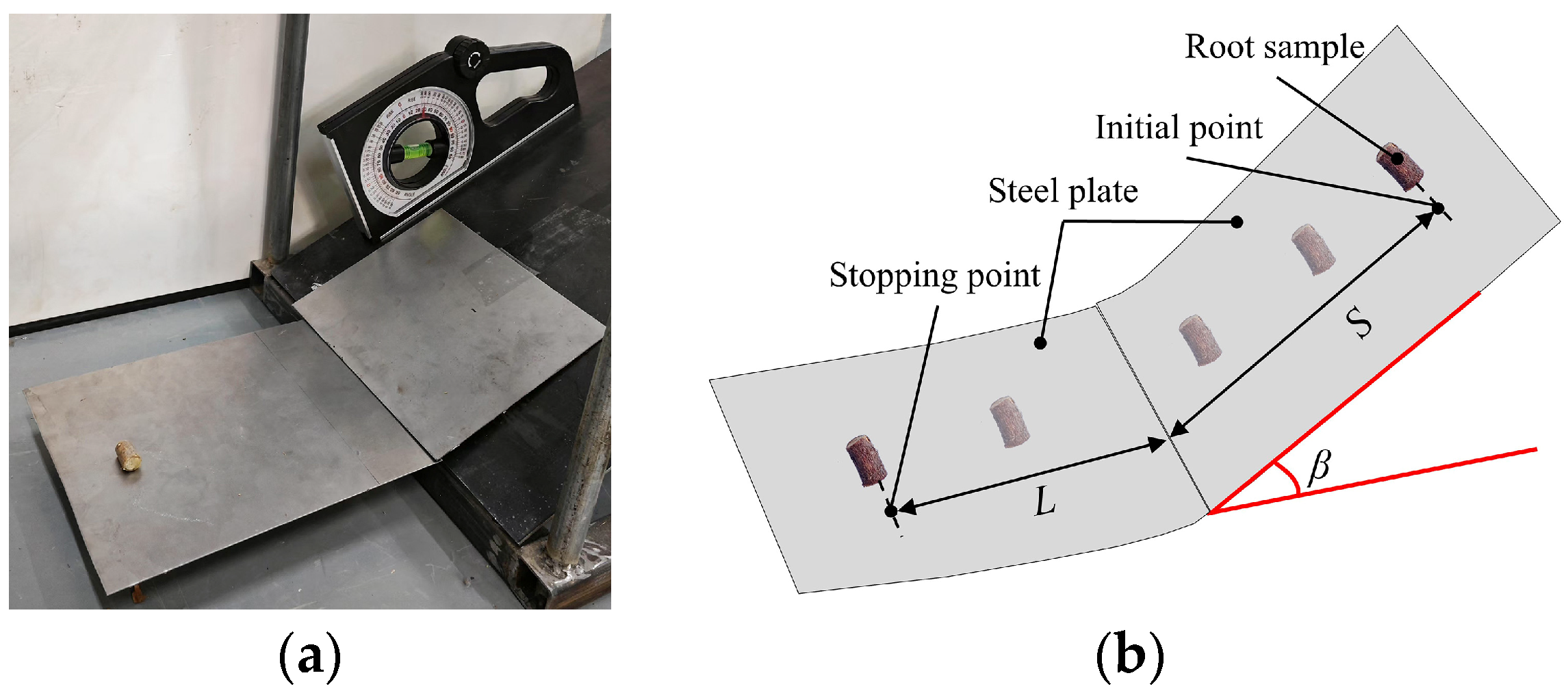
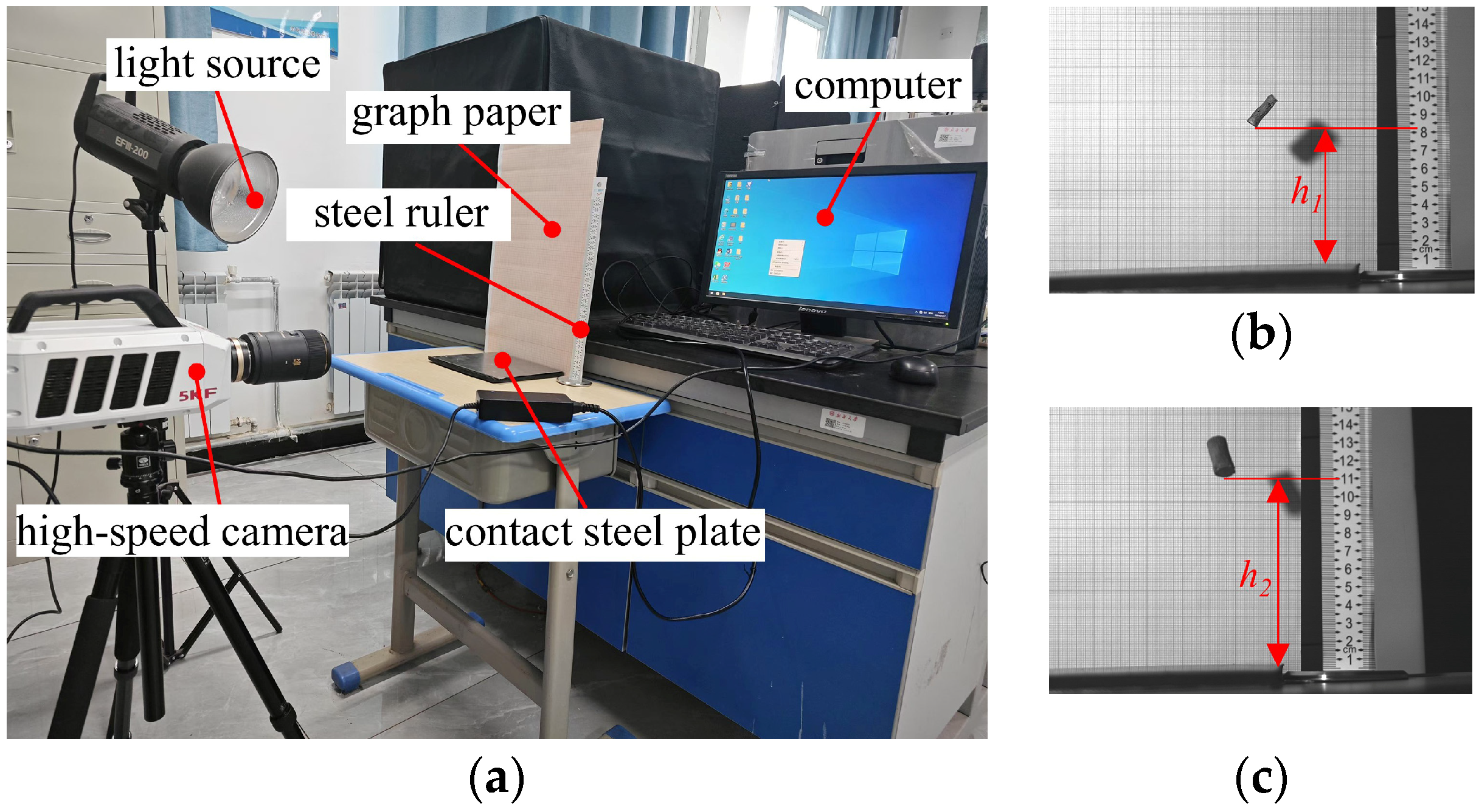
The friction coefficient and coefficient of restitution were assessed through friction characteristic tests and root drop rebound tests [24], as illustrated in Figure 2 and Figure 3. The average parameter values include the static friction coefficients of 0.616 for primary root–steel interfaces and 0.563 for lateral root–steel interfaces, along with rolling friction coefficients of 0.0847 and 0.0503, respectively. The coefficients of restitution were found to be 0.612 and 0.519. The data indicate that the friction and restitution coefficients for primary and lateral roots are closely aligned, allowing for the application of identical values in subsequent DEM contact parameter settings. Following Refs. [10,20] and experimental measurements, the cotton root–steel interface exhibits static friction coefficients ranging from 0.563 to 0.616, rolling friction coefficients in the range of 0.05–0.085, and coefficients of restitution varying from 0.429 to 0.612.

2.2. Physical Test of the Cotton Roots Stacking Angle

During the stacking process of roots, their surfaces experience various motion states such as contact, friction, and flow, which comprehensively reflect parameters like the contact interactions among roots and between roots and steel. The stacking angle of the cotton roots was measured using the cylinder lifting method. The steel cylinder had an inner diameter of 120 mm and a height of 240 mm. The test samples included cotton taproots with a length of 25 mm and average diameters of 4 mm, 5.8 mm, and 7 mm, as well as lateral roots measuring 25 mm and 30 mm in length, with an average diameter of 3.16 mm, totaling 600 root samples. The cylinder was slowly lifted at a constant speed of 0.05 m/s, and a front-view image was captured once the cotton stalk roots pile had stabilized. The original images were first converted to grayscale on one side using Matlab 2024a software, and adaptive thresholding was applied for image binarization. The processed images were then imported into Photoshop, where the ‘Pen Tool’ was used to extract the image edge contours and generate smooth path curves. Finally, the resulting edge images were imported into Origin 2024 software, and the image digitization tool was used to extract the coordinates of the edge lines point by point, followed by curve fitting [25]. The image processing steps are illustrated in Figure 4. For each trial, the average stacking angles on both the left and right sides were recorded. The experiment was repeated 10 times, yielding a final average repose angle of 26.61°.

2.3. Measurement of Cotton Roots Shear Mechanical Properties

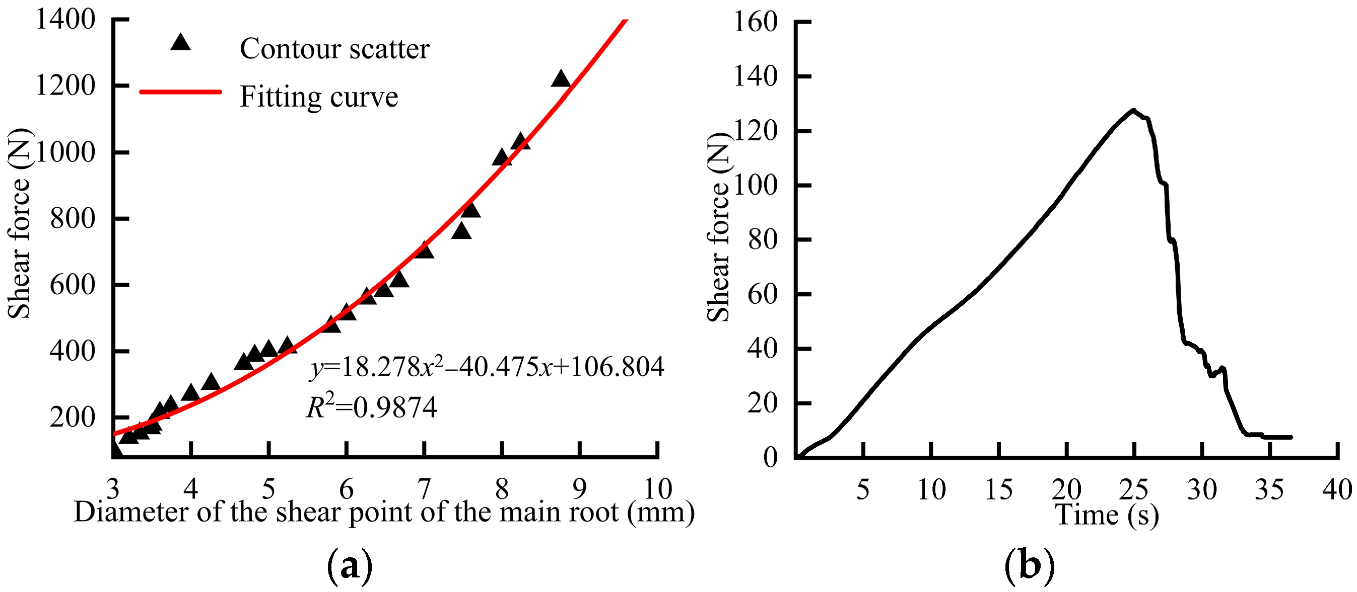
Root shear tests were conducted using the WDW-50M microcomputer-controlled electronic universal testing machine. The diameter of the primary root samples at the shear point ranged from 3 to 8.76 mm, whereas the average diameter of the lateral root specimens was measured at 3.16 mm. Each group comprised 20 root samples, each subjected to two shear tests, with the average peak shear force of the roots taken as the final result. The loading rate and return speed of the testing machine were both set at 100 mm/min, and data integration was conducted after completing the tests. The peak shear force for the primary roots varied from 102.174 N to 1215.233 N.
Based on the analysis results depicted in Figure 5a, the shear force grows as the diameter of the shear point increases, demonstrating a quadratic relationship between the two. This quadratic relationship can be stated by Equation (1), with a determination coefficient R2 of 0.9874. As illustrated in Figure 5b, the cotton root initially experiences a linear elastic phase, during which the shear force gradually increases. This phase is followed by the fracture stage, where the shear force peaks and then rapidly declines.
y 1 = 18.278 x 2 40.475 x + 106.804

2.4. Establishment of the Discrete Element Simulation Model

2.4.1. Selection of the Discrete Element Contact Model

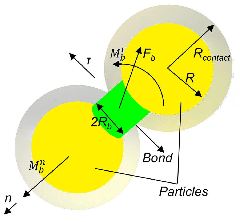
The default Hertz–Mindlin no-slip contact model in EDEM 2024.1 software was selected to conduct the stacking angle simulation test on cotton roots. This model effectively quantifies the contact parameters between particle models as well as between these models and contact materials [26]. To perform shear and tensile simulation tests on cotton roots, the Hertz–Mindlin with bonding model was utilized. This model operates on the principle of creating bonding connections between particles within the discrete element software, which generates cohesive forces and adds a degree of flexibility to the system. The bonding connections have specific mechanical properties that influence the model’s behavior. A representation of the bonding connections between particles is illustrated in Figure 6. When an external force is applied, the model experiences deformation and generates internal stress. If the internal stress surpasses the threshold limit between the units, the bonding connections between them fail, resulting in a loss of bonding efficiency and causing the units to separate. This process effectively simulates the biomechanical characteristics of cotton roots.
At the TBOND moment, the particles are bonded, and prior to this, they interact through the default Hertz–Mindlin contact model. As time steps increase, the bonding forces Fn, Ft and the torques Tn, Tt begin to rise from zero according to Equation (2) [27].
δ F n = v n S n A δ t δ F t = v t S t A δ t δ T n = w t S t J δ t δ T t = w t S n J δ t / 2
where A is the contact area, mm2; J is the moment of inertia, mm4; Sn and St are the normal and shear stiffness per unit area, N/m3, respectively; vn and vt are the normal and shear velocities of the particles, m/s, respectively; wn and wt are the normal and shear angular velocities, m/s, respectively; and δt is the time step, s.
When the normal and shear forces exceed a certain threshold value, the bond is broken. The maximum values of normal and shear stiffness are defined in Equations (3) and (4) [28]. Therefore, the fracture of cotton roots can be simulated through the failure of bonding bonds.
σ m a x < F n A + 2 T t J R B
τ m a x < F t A + T n J R B

2.4.2. Root System Modeling Based on the 3D Scanning

In precision agriculture, modeling subsurface root systems has emerged as a significant technical challenge. Three-dimensional scanning-based methodologies substantially enhance the geometric accuracy of root architecture characterization. When integrated with DEM rapid-fill modeling, this approach not only enhances modeling efficiency but also fosters a more nuanced understanding of root dynamics. Accurate simulation of root structures is critical for the design of DEM-optimized agricultural machinery focused on rhizosphere operations and on visualizing micromechanical interactions at root–soil interfaces.
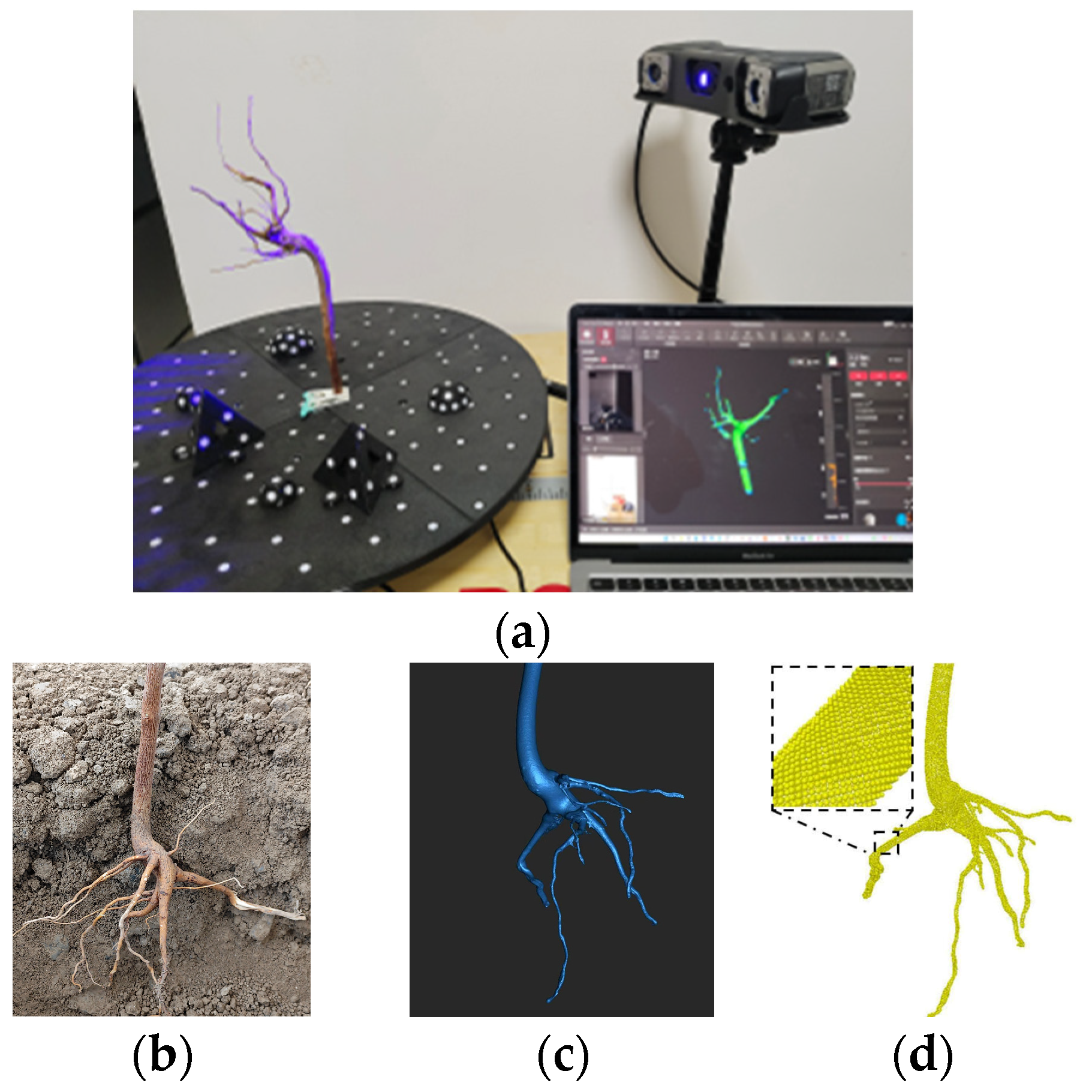
This research utilizes a Revopoint MetroX laser 3D scanner to analyze selected cotton root specimens that meet benchmark parameters. Multi-angle high-speed scanning captures high-density root surface point cloud data. Subsequent processing with Revo Scan 5.6.5 software implements Poisson surface reconstruction, resulting in topologically structured parametric NURBS geometric models. A secondary development using the Python 3.12 API was performed to discretize the root geometry into cubic voxels with a resolution of 3.1 mm. The centroid coordinates of these voxels were then exported and mapped into the discrete element model as spherical particles, thereby establishing a direct geometric and topological correspondence between the voxel grid and the particle system. This voxel-based approach ensures a uniform and regular particle distribution while still preserving the essential morphological characteristics of the root system. Curved or irregular parts of the roots were approximated by adjacent voxel elements, which simplifies the geometry while maintaining computational efficiency and modeling fidelity. Based on a comprehensive consideration of the actual morphology of cotton roots, computational efficiency, and model accuracy, standard spherical particles with a radius of 0.5 mm were selected for modeling, and the contact radius was set to 0.6 mm. The discrete element-based modeling of the cotton root system has been illustrated in Figure 7.

2.4.3. Establishment of the Simulation Model for the Stacking Angle Test

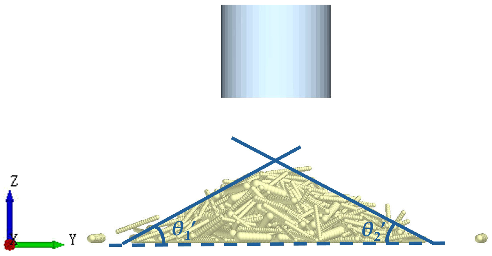
In the stacking angle simulation, the root system was modeled as a single-chain rod composed of spherical particles to capture the overall contact mechanical response. Studies have shown [7] that increasing the number of spheres only marginally improves the accuracy of stacking angle simulations while significantly increasing computational time. Therefore, employing a single-chain rod model ensures efficient simulations without compromising accuracy. A bottomless cylinder, identical to the one used in the actual experiment, is constructed in EDEM, and the intrinsic parameters for steel are applied accordingly. Subsequently, two dynamic particle factories are integrated within the cylinder to generate cotton root samples of varying shapes. The generation rate for both particle factories is established at 1000 particles per second, culminating in a total generation quantity of 600. Once the root particles are created, they are allowed to remain stationary for 1.5 s to achieve a static state, after which the cylinder is elevated at a consistent speed of 0.05 m/s.
Following the completion of the root stacking, the “Protractor” tool in the post-processing module is employed to assess the average stacking angle from the −X view in the simulation experiment. The simulation model of the stacking angle has been depicted in Figure 8. In the stacking angle simulation tests, the contact parameters were comprehensively determined based on pre-test results, physical measurement data, and references [8,21], as shown in Table 3.

2.4.4. Establishment of the Cotton Roots Shear Simulation Model

In the root shear simulation test, a structured multi-layer particle model was adopted to construct the root samples, enabling a more realistic representation of the mechanical properties of root material and its heterogeneous deformation under shear forces. This modeling approach explicitly simulates the progressive breakage of bonding bonds between particles, thereby facilitating accurate capture of the structural evolution and failure mechanisms of roots during the shearing process. A DEM of the cotton root was developed by filling standard spherical particles, each with a radius of 0.5 mm, in a regular pattern. The spatial distribution of these particles was generated via Python 3.12 scripting to ensure a precise arrangement. During the simulation tests, the speed of the shear tool was maintained in accordance with the actual test conditions. The simulation time step was established at 25% of the Rayleigh time step, with a data saving interval set to 0.01 s, and the grid size configured to be three times the minimum particle radius. The cotton root shear simulation model has been illustrated in Figure 9. The range of root bonding parameters was determined by examining the parameters from similar material models [8,21,29,30] and conducting preliminary simulation tests, as presented in Table 4.

2.5. Parameter Calibration Method

2.5.1. Plackett–Burman Test

To efficiently identify and screen the key contact parameters that significantly influence the stacking angle while keeping the number of experimental measurements to a minimum, the Plackett–Burman experimental design was first applied for parameter selection. The simulated root stacking angle (θ′) served as the response value, while the Plackett–Burman experimental design selected key factors including the root–root restitution coefficient (X1), static friction coefficient (X2), rolling friction coefficient (X3), root–steel restitution coefficient (X4), static friction coefficient (X5), and rolling friction coefficient (X6). The codes “+1” and “−1” represent the high and low levels of these factors, respectively, with the corresponding factor values detailed in Table 3.

2.5.2. Steepest Ascent Test

After the significant influencing factors were identified, the steepest ascent test was conducted to quickly converge toward the optimal region by following the gradient direction of these significant parameters. The direction of ascent is determined based on the positive and negative effect values of significant factors in the experimental Pareto chart, and an experimental gradient is constructed along this direction. Finally, the stacking angle simulation experiments are conducted following the steepest ascent design, and the errors between the simulated and measured stacking angle values for each group are calculated.

2.5.3. Box–Behnken Test

The Box–Behnken experimental design is a widely used experimental approach in response surface methodology, enabling the efficient construction of second-order response surface models to identify the optimal combination of significant factors and achieve the best response. Based on the results of the Plackett–Burman test and the central point determined by the steepest ascent test, a Box–Behnken design model is established with the stacking angle as the response value, and a quadratic polynomial regression model is constructed to describe the relationship between the response and the influencing factors.

2.5.4. CCD Test

Compared to the contact model, the bond model involves fewer parameters, so we adopted the one-step Central Composite experimental design for calibration. This approach provides comprehensive second-order model information, including all interaction and quadratic effects, thereby fulfilling the requirements for precise optimization of bond parameters. The four bonding parameters within the selected Hertz–Mindlin bonding model were calibrated, with the ranges of various factors documented in Table 4. Each factor was organized at five levels: −α, −1, 0, +1, and +α, where α represents the distance to the axial point and is calculated according to Equation (5). A four-factor, five-level experimental design was formulated with peak shear (Fmax) as the response variable. The experimental factors were encoded based on the mapping between the code values of [−2, +2] and the corresponding factor ranges (i.e., [min, max]), as illustrated in Table 5.
α = ( 2 k ) 1 4
where k is the number of factors.

3. Results and Discussion

3.1. Calibration of the Contact Parameters

3.1.1. Plackett–Burman Test Analysis

The Plackett–Burman test was employed to conduct a significance screening analysis of the fundamental contact parameters. A total of 12 experimental groups were devised, with each group undergoing three simulations. Measurements of the left and right stacking angles were taken from the −X view, resulting in 72 measurements overall. The average value was evaluated and utilized as the simulated stacking angle. The details of the Plackett–Burman experimental design and results are provided in Table 6, while the analysis of variance (ANOVA) for the Plackett–Burman test has been summarized in Table 7.
In Table 7, the p-values were utilized to assess the significance of each experimental factor or variable on the experimental response. A commonly accepted threshold is p < 0.05, which indicates that a factor has a significant impact on the response with a 95% confidence level. In the case of p < 0.01, the factor is deemed to have a highly significant effect at the 99% confidence level. The model p-value was determined to be 0.0144, confirming that the model is statistically significant. Among the variables examined, the p-values associated with the root–root static friction coefficient (X2), the root–root rolling friction coefficient (X3), and the root–steel static friction coefficient (X5) were all less than 0.05, signifying that these three factors have substantial impacts on the stacking angle. Consequently, factors X2, X3, and X5 were subjected to further analysis using the steepest ascent test.

3.1.2. Steepest Ascent Test Analysis

From the Pareto chart of standardized effects (see Figure 10), it is clear that factor X3 has a positive influence on the stacking angle, indicating that as X3 increases, the stacking angle also rises. Factors X5 and X2 similarly demonstrated positive effects. The hierarchy of significance for the factors impacting the stacking angle is as follows: X3 > X5 > X2. Consequently, in the experimental design, factors X2, X3, and X5 were arranged in an ascending manner. For the factors deemed non-significant, mid-level values were utilized. The experimental index used to evaluate performance was the relative error between the simulated stacking angle (θ′) and the actual stacking angle (θ). The formula for calculating the relative error is outlined in the following form:
φ = θ θ θ × 100 %
where φ is the relative error of stacking angle, %; θ′ is the simulated stacking angle, °; θ is the actual stacking angle, °.
As presented in Table 8, the relative error of the stacking angle initially decreased before increasing as X2, X3, and X5 were raised. Test 3 demonstrates the smallest relative error, aligning closely with the physical value; therefore, it has been designated as the central level. In the subsequent Box–Behnken design, the factor levels from Tests 2 and 4 were then utilized as the lowest and highest levels, respectively.

3.1.3. Box–Behnken Test Analysis

To optimize the combination of contact parameters, we conducted a response surface analysis utilizing a three-factor, three-level Box–Behnken experimental design. The primary experimental indicator was the relative error (φ) between the simulated and actual stacking angles. A total of 17 experiments were carried out, with each experiment repeated three times to ensure accuracy, and then the corresponding average values were recorded as the results. The details of the experimental design and results are summarized in Table 9. By fitting the response surface experimental results, we could develop a second-order regression model that elucidates the relationship between the stacking angle and the three significant factors as follows:
y 2 = 26.80 + 0.51 X 2 + 1.94 X 3 + 1.50 X 5 + 0.25 X 2 X 3 0.10 X 2 X 5 + 0.2950 X 3 X 5 0.4125 X 2 2 0.5825 X 3 2 + 0.2775 X 5 2
The analysis results of variance (ANOVA) based on the quadratic regression model have been given in Table 10. The coefficient of determination (R2) was measured at 0.9952, with a p-value of less than 0.0001, indicating that the model is highly significant. Additionally, the lack-of-fit test yielded no significant results, suggesting that the model demonstrated a robust fit within the regression region. Based on the model p-values, the root–root static friction coefficient (X2), the root–root rolling friction coefficient (X3), and the root–steel static friction coefficient (X5) each exhibited a highly significant effect on the root stacking angle. Furthermore, the quadratic terms X 2 2 and X 3 2 also exhibited highly significant effects, while X 5 2 was found to be significant. Regarding interaction effects, X2X3 and X3X5 were significant, whereas X2X5 did not show significance.
The interactions between various factors were analyzed by means of Design-Expert 13 software, and the corresponding response surface plots for these factors were generated, as illustrated in Figure 11. As illustrated in Figure 11a, when the root–root rolling friction coefficient (X3) was held constant, the stacking angle gradually increased as the root–root static friction coefficient (X2) increased. On the contrary, when X2 was held constant, the three-dimensional response surface plot revealed that the stacking angle increased more significantly with an increase in X3, indicating that the impact of X3 on the stacking angle was more pronounced than that of X2. As depicted in Figure 11b, when the root–steel static friction coefficient (X5) was maintained constant, the stacking angle progressively increased with the rise in the root–root static friction coefficient (X2). Conversely, when X2 was fixed, the three-dimensional response surface plot demonstrated that the stacking angle exhibited a more substantial increase with rising X5, indicating that the influence of X5 on the stacking angle was more significant than that of X2. As illustrated in Figure 11c, when the root–root rolling friction coefficient (X3) was constant, the stacking angle was observed to incrementally rise with the increase in the root–steel static friction coefficient (X5). When X5 was held constant, the increase in the stacking angle became more pronounced in the three-dimensional response surface plot as X3 increased, signifying that the effect of X3 on the stacking angle was more significant than that of X5.
In summary, among the three significant factors, the order of their significance was X3 > X5 > X2. Specifically, X3 primarily regulates the difficulty of rolling between roots, directly affecting whether the pile structure is loose or compact; X5 determines the ‘anchoring’ effect at the base of the piling, playing a key role in overall stability. Furthermore, X3 dominates the internal mechanical behavior of the pile by influencing the ‘locking’ effect between particles, while X5 enhances the basal anchoring effect. Together, these two factors govern the variation trend of the stacking angle. In contrast, although X2 affects the ease of sliding between roots, due to the complexity of root morphology and their interlocking nature, actual sliding behavior is often replaced by rolling or mechanical interlock mechanisms, thereby rendering its dominant influence on the stacking angle trend weaker than that of X3 and X5.

3.1.4. Contact Parameters Optimization and Simulation Test Verification

Based on the physical experiment results, the target value for the stacking angle was set equal to 26.61°. The “Optimization” module in Design-Expert 13 software was then utilized to solve for the optimal values of the regression equation. This yields the following parameter combination as the best response: root–root static friction coefficient of X2 = 0.571, root–root rolling friction coefficient of X3 = 0.18, and root–steel static friction coefficient of X5 = 0.583. The simulation experiments for the stacking angle were conducted using EDEM software based on the aforementioned parameter combination. The resulting simulated stacking angles were obtained as 26.05°, 26.14°, 27.09°, 26.43°, and 26.77°, with an average value of 26.496°. These results exhibited a minimal relative error of 0.43% compared to the physical experiment results, demonstrating the high reliability of the simulation tests and establishing a parameter foundation for the further calibration of the bonding model. Moreover, compared to the approach in reference [21], where the cotton rootstalk–soil mixture was treated as a whole for contact parameter calibration, this study did not consider the stalk and root system as a single entity. Instead, we conducted an independent and systematic calibration specifically for the root component. As a result, the obtained optimal contact parameter range for the roots was more precise, and the relative error was lower than the 2.36% reported in reference [21].

3.2. Calibration of the Bonding Parameters

3.2.1. CCD Test Analysis

In both simulation and physical shear experiments, the diameter of the shear zone was kept at 5.8 mm. The shape of the primary root close to this region was approximately cylindrical. Therefore, the root’s shape was idealized as a cylinder for constructing the cotton root shear model. In total, 27 simulation experiments were performed. Among them, the CCD comprised three groups; each group was replicated three times, and the main results obtained were appropriately averaged. The CCD experimental design and results are presented in Table 11, whereas the analysis of variance (ANOVA) results are provided in Table 12.
As demonstrated in Table 12, the coefficient of determination (R2) for the model was estimated to be 0.9960, and the adjusted R2 was 0.9913. The model’s p-value was less than 0.0001, whereas the p-value for the lack-of-fit term was 0.0852, indicating that the model’s overall fit was statistically acceptable. In this model, both normal contact stiffness (X7) and shear contact stiffness (X8) exhibited highly significant impacts on the peak shear force; the quadratic term ( X 7 2 ) demonstrated a highly significant effect; and the interaction term (X7X8) illustrated a significant effect. The experimental data were fitted using quadratic multiple regression, yielding the regression Equation (8).
y 3 = 467.12 + 23.05 X 7 + 5.89 X 8 + 0.1050 X 9 + 0.1733 X 10 + 1.58 X 7 X 8 + 0.2512 X 7 X 9 + 0.8512 X 7 X 10 + 0.5675 X 8 X 9 + 0.6450 X 8 X 10 + 0.6137 X 9 X 10 1.72 X 7 2 3.22 X 8 2 + 0.0310 X 9 2 + 0.4910 X 10 2
Since the critical normal stress (X9), critical shear stress (X10), their interactional term (X9X10), and the quadratic terms ( X 9 2 , X 10 2 ) were not statistically significant in the shear test, the values of these non-significant factors were fixed at their intermediate levels. After excluding the non-significant terms, the final binary regression equation is presented in Equation (9).
y 4 = 467.82 + 23.05 X 7 + 5.89 X 8 + 1.58 X 7 X 8 1.85 X 7 2 3.35 X 8 2
By setting the actual peak shear as the target value, the regression equation was solved to obtain the optimal parameter combination: normal contact stiffness (X7) was 3.57 × 10¹⁰ N/m3, shear contact stiffness (X8) was 3.84 × 10¹⁰ N/m3, critical normal stress (X9) was 25 MPa, and critical shear stress (X10) was 30 MPa. Under this parameter combination, five shear simulation tests were conducted, and the peak shear forces were 479.52 N, 480.35 N, 481.59 N, 484.66 N, and 475.87 N, respectively, and the average peak shear force was 480.40 N. The relative error between the simulated value and the actual value of 474.62 N was 1.22%, demonstrating that the proposed shear model exhibits high reliability and the calibrated bonding parameters are accurate. The physical shear test of cotton roots and the corresponding bond failure process are illustrated in Figure 12.

3.2.2. Bonding Parameters Optimization and Simulation Test Verification

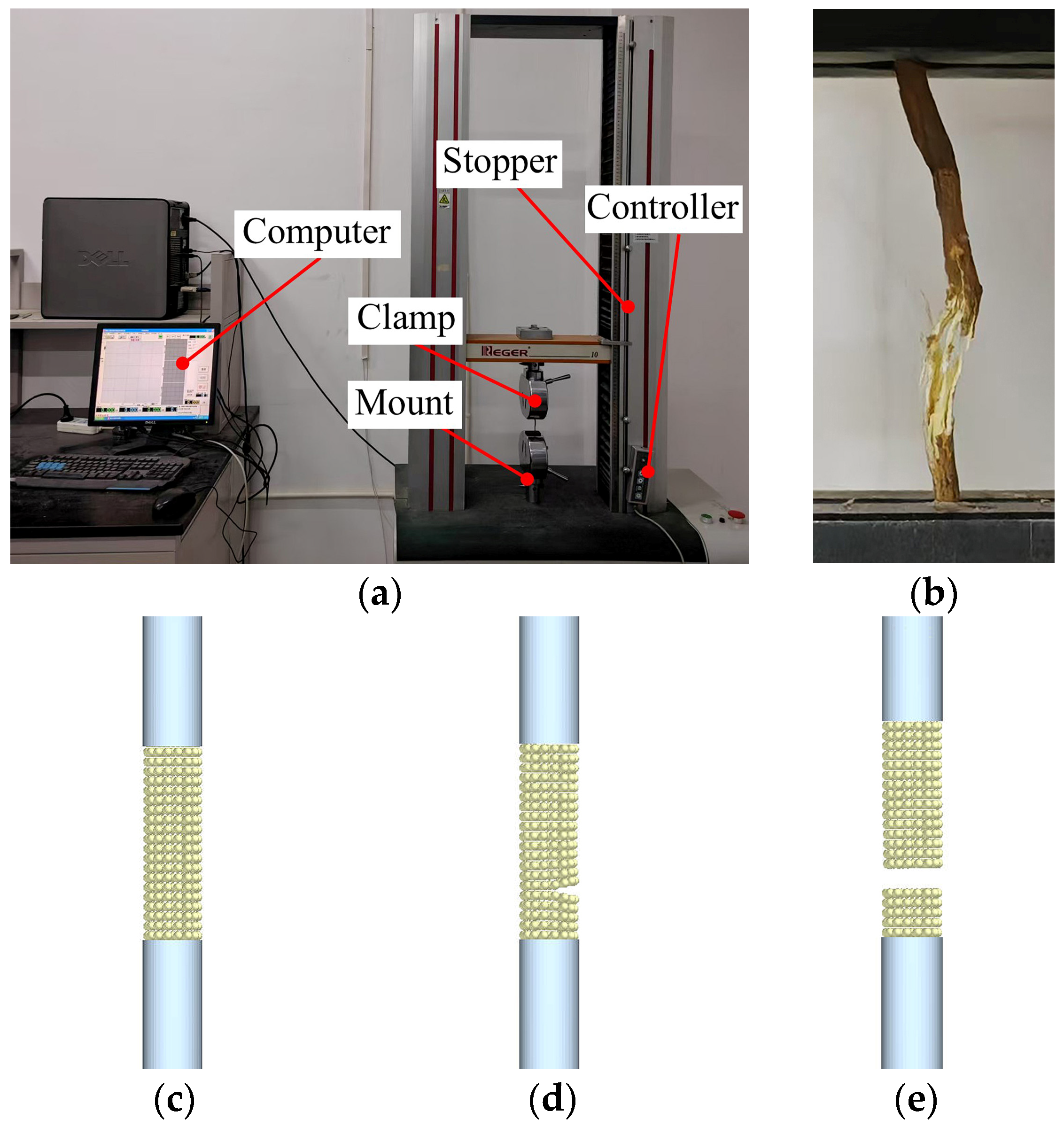
To further validate the reliability of the calibration results for the bonding parameters in the established DEM for the cotton root, tensile verification tests were conducted on the lateral roots, as illustrated in Figure 13. In conventional tensile simulation tests, one end of the test object is typically fixed using the “Fixed Velocity” method, while the other end is clamped with a bottomless cylinder whose diameter is slightly smaller than that of the test object. However, during several preliminary tests, slight relative slippage between the cylinder and the test object was observed, leading to an increase in the relative error of the measured tensile force. With advancements in EDEM software, the present study employed the Rigid Link function in EDEM version 2024.1, activating it to “on contact” to ensure that one end of the test object remained securely fixed to the cylinder throughout the stretching process.
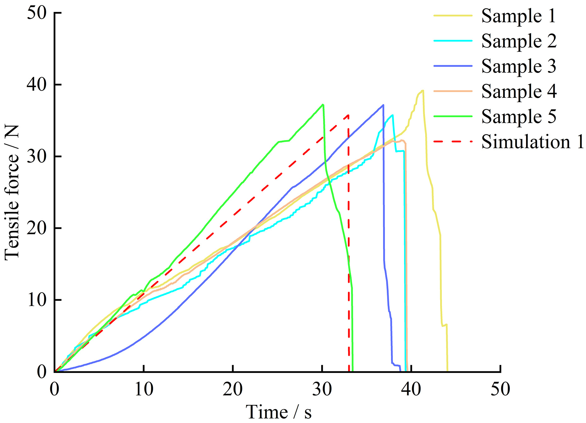
Prior to the rupture of the cotton root, the tensile force exhibited a linear relationship with loading time, consistently increasing as the loading duration progressed. Before reaching the maximum tensile force, the root underwent two distinct stages: partial fracture and complete cross-sectional fracture, after which the tensile force declined sharply. Figure 14 illustrates the variation in tensile force during both the simulated and actual stretching processes. As depicted in the figure, the overall trends of the curves are consistent. The average maximum tensile force measured in the actual tensile test was obtained as 36.287 N, whereas the simulated value was calculated as 35.780 N, leading to a relative error of 1.40%. These results also reveal the feasibility of the calibrated bonding parameters. The mechanical properties of roots during tensile loading, including their ultimate tensile force, failure modes, and deformation characteristics, provide critical evidence for validating the mechanical strength and toughness reflected by the root model. However, roots are tightly intertwined with the surrounding soil to form a root–soil composite, which jointly bears external loads. This synergistic mechanism highlights that relying solely on tensile tests may not fully capture the mechanical behavior of roots under actual harvesting conditions. Therefore, supplementing with root pull-out tests is of significant importance, as it more accurately simulates the response mechanism of the root–soil interface under complex loading conditions.

3.3. Field Trial Validation

In order to further verify the reliability of the aforementioned parameters, a verification test for root uplift force was conducted. The test site was situated in Awati Township, Korla City, Bayin’guoleng Mongol Autonomous Prefecture, Xinjiang (86°09′ E, 41°16′ N). At this time, the cotton harvesting operation had been completed. The tensile force measuring device comprised a digital dynamometer, a wire rope, and a cotton straw clamping device. The five-point method was employed to perform cotton straw pull-up force tests at five designated plot points, with the clamping position set at a vertical height of 80–100 mm above the ground and a pull-up angle of 60° [31]. A total of ten sets of uprooting force tests were conducted at each plot; the roots of the uprooted cotton stalks were cut, numbered, labeled, and subsequently transported back to the laboratory. The average pulling force was calculated to be 416.19 N. The numbered and labeled root systems were dimensionally measured, and root systems that closely resembled the scanned model were selected, yielding an average pulling force of 436.39 N.
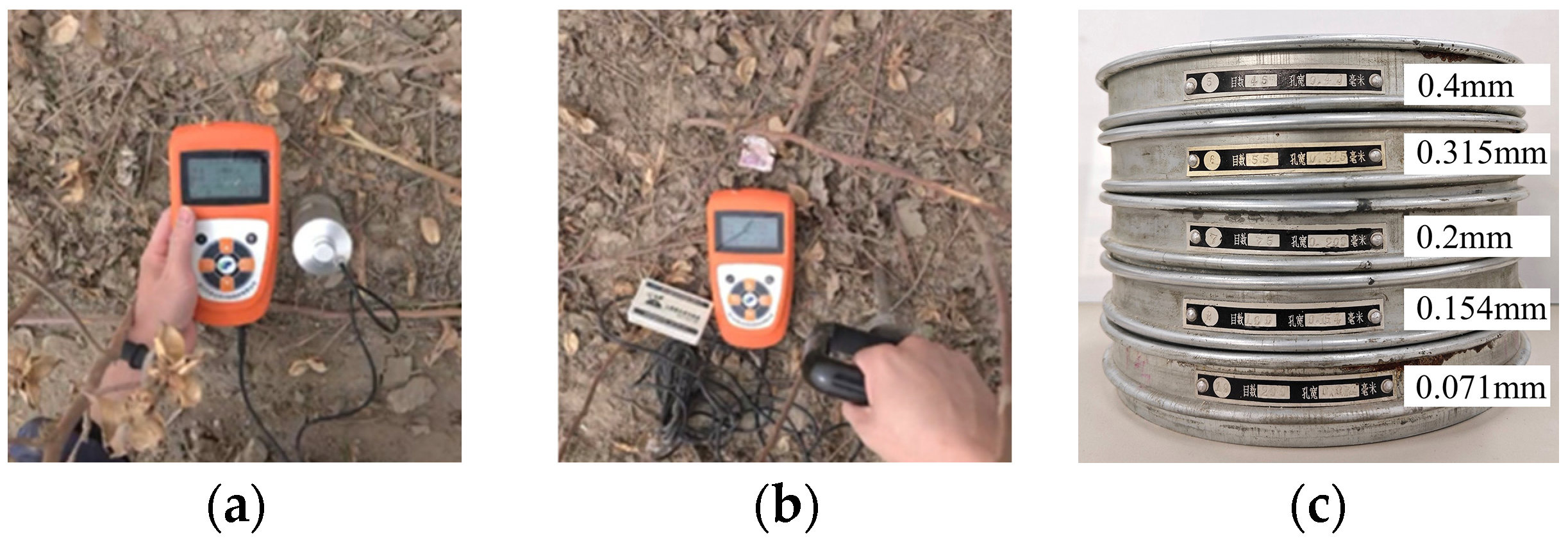
In addition, the field test is illustrated in Figure 15. To facilitate the accurate selection of soil DEM parameters, the grain size distribution, compactness, and water content of the cotton field soil were measured; the results of the measurement test are presented in Figure 16. The soil was classified as sandy loam, with a compactness of 447.35 kPa and an average water content of 21.4%. Based on the soil type, measurement results, and the relevant literature [21,32,33], the soil DEM input parameters were established through a series of preliminary simulation experiments (see Table 13).
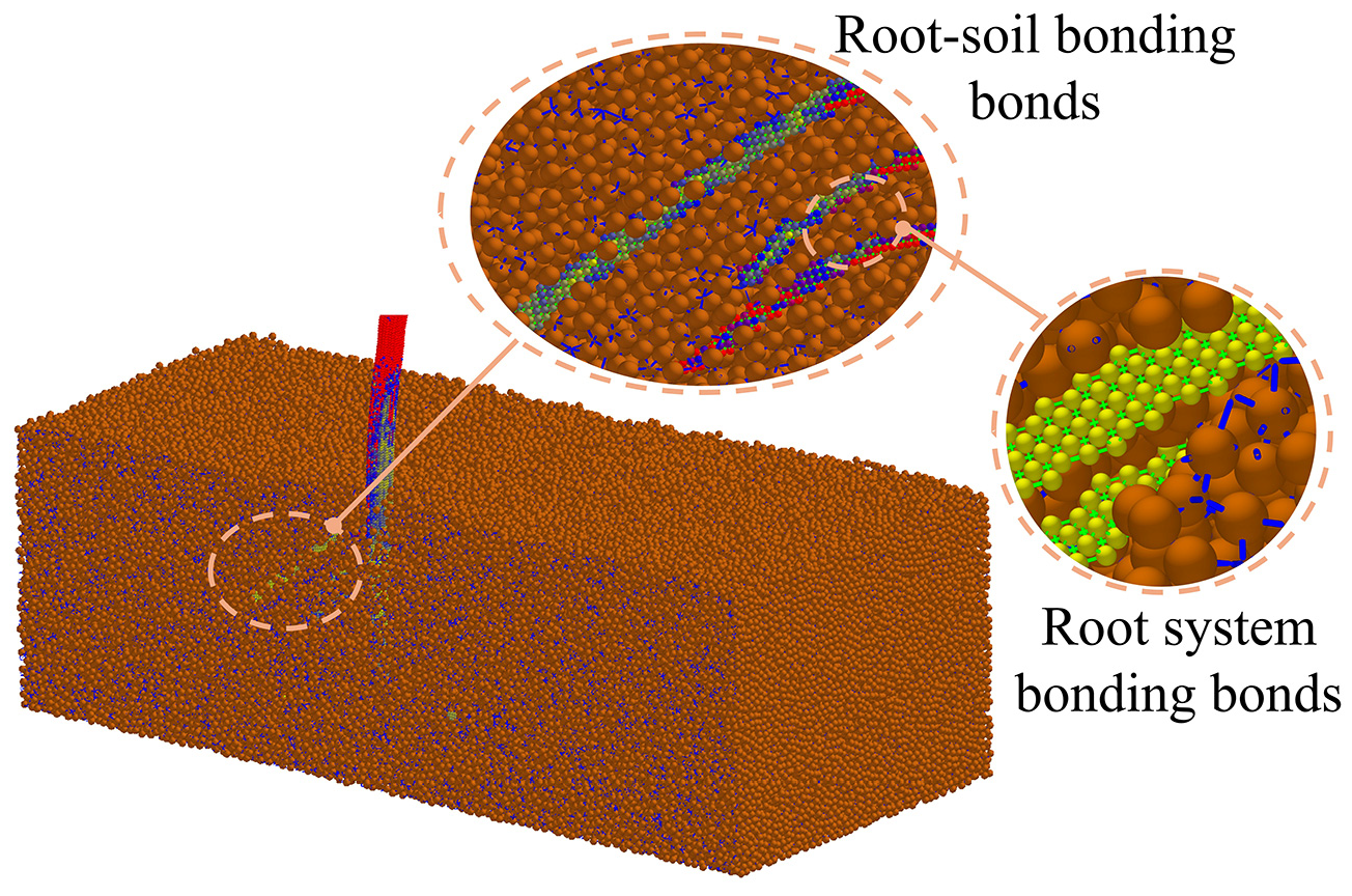
In the pull-up force simulation test, the root system-root system and root system-soil interfaces were linked using bonding keys, as illustrated in Figure 17. The simulation test was conducted five times, yielding an average pull-up force of 452.79 N, which closely aligned with the measured value of 436.39 N, resulting in a relative error of 3.76%. This outcome suggests that the calibrated contact and bonding parameters were effectively optimized and that the constructed root system model accurately simulated the mechanical behavior of cotton straw during the pull-up process. During the EDEM-based visualization of the simulation, it was observed that the formation of the failure mode in the cotton root system during the pull-out process depends on the relative relationship between the bonding strength at the cotton root–soil interface and the intrinsic strength of the cotton root system itself. By analyzing the stress distribution and structural responses at different stages, this study can provide a targeted parameter optimization basis for the design of root pull-out machinery.

4. Conclusions

In this study, a comprehensive model of the cotton root system was developed utilizing the discrete element method (DEM) and 3D laser scanning technology. The contact and bonding parameters of the established DEM for the root system were systematically calibrated and optimized through the integration of physical and simulation tests, while simultaneously conducting verification tests of the root system’s pull-up force. The major results obtained can be summarized as follows:
(1)
This study, based on systematic real-time measurements of cotton root systems during harvest, successfully gathered critical data, including profile structure parameters, friction characteristic parameters, stacking angles, and mechanical characteristic parameters of the root systems. The detailed dimensions of the root system were obtained through physical measurements, revealing static friction coefficients between cotton roots and steel in the range of 0.563 to 0.616, rolling friction coefficients between 0.05 and 0.085, and restitution coefficients ranging from 0.429 to 0.612. Moreover, the average stacking angle, determined via stacking angle tests, was found to be 26.61°. The peak shearing force of the main root with varying axial diameters, measured through shear tests, ranged from 102.174 N to 1215.233 N, while the average peak shear force of lateral roots was recorded at 146.077 N. The average maximum tensile breaking force identified in lateral root tensile tests was 36.287 N. Using these foundational physical parameters, the cotton root bonding model was constructed by integrating the root structure derived from the 3D laser scans and utilizing the particle fast-filling function within EDEM software.
(2)
The parameters of the contact model and bond model were calibrated by establishing an optimization procedure with the stacking angle and peak shear force as key response indicators. In the contact model, the static friction coefficient between root–root, rolling friction coefficient, and restitution coefficient between root–steel significantly influenced the stacking angle. An optimal parameter set, determined through Box–Behnken response surface optimization tests, was identified as 0.571, 0.180, and 0.583. The simulated stacking angle also achieved with these parameters was 26.496°, with a relative error of only 0.43% compared to the actual stacking angle. In the bonding model, the effects of normal contact stiffness and shear contact stiffness on the peak shear force were significant, leading to an optimal parameter solution of 3.57 × 10¹⁰ N/m3 for normal contact stiffness and 3.84 × 10¹⁰ N/m3 for shear contact stiffness. The simulated peak shear force of the coaxial diameter main root under this parameter combination was 480.40 N, matching the actual measurement exactly, with a relative error of just 1.22%. Additionally, the simulated maximum destructive tensile force of the lateral root was found to be 32.780 N, presenting a relative error of 1.40% when compared to the measured value.
(3)
Utilizing the calibrated root model parameters, a simulation model representing root–soil complexes was constructed to reflect actual harvesting conditions, enabling the verification of root pull-up force. The results obtained indicated an average pull-up force of 452.79 N across five trials, which was comparable to the field test value of 436.39 N, resulting in a 3.76% relative error. This evidence highlights the validity of the root model in simulating complex root–soil interactions. The research findings provide a theoretical foundation and reliable data to support the structural design and optimization of operational parameters for cotton stalk harvesting equipment.
(4)
The modeling approach proposed in this study provides a feasible and effective flexible root model for the simulation-based design and optimization of whole-stalk cotton stalk harvesters. Additionally, the parameter calibration and optimization have further enriched the DEM parameter database in this field. It should be noted that the field experiments on root extraction force were conducted under specific soil conditions (sandy loam) and moisture content. Whether the root model can maintain its accuracy after adjusting soil-specific parameters requires further validation through more extensive testing. To enhance the applicability of the parameters across different soil types and moisture levels, follow-up studies will include systematic sensitivity analyses involving various cotton field soil types and different moisture gradients. This will help verify and extend the reliability and generalizability of the root model.

Author Contributions

Conceptualization, Y.Y., R.X. and Y.B.; methodology, R.X. and Y.B.; software, R.X.; validation, R.X. and H.X.; formal analysis, Y.Y.; investigation, R.X.; resources, W.M.; data curation, R.X.; writing—original draft preparation, R.X.; writing—review and editing, Y.Y., R.X. and L.G.; visualization, R.X.; supervision, W.M.; project administration, R.X. All authors have read and agreed to the published version of the manuscript.

Funding

This study was funded by the Youth Science Foundation under Grant 2022D01B91. The authors also acknowledge the Key Laboratory of Xinjiang Intelligent Agricultural Equipment, China, and the College of Mechanical and Vehicle Engineering, Chongqing University, for their assistance with the instruments and equipment.

Institutional Review Board Statement

Not applicable.

Data Availability Statement

The data presented in this study are available on request from the corresponding author.

Conflicts of Interest

The authors declare no conflicts of interest.

References

  1. Cai, C.; Wang, Z.; Ma, L.; Xu, Z.; Yu, J.; Li, F. Cotton stalk valorization towards bio-based materials, chemicals, and biofuels: A review. Renew. Sustain. Energy Rev. 2024, 202, 114651. [Google Scholar] [CrossRef]
  2. Zhu, Y.; Zheng, B.; Luo, Q.; Jiao, W.; Yang, Y. Uncovering the drivers and regional variability of cotton yield in China. Agriculture 2023, 13, 2132. [Google Scholar] [CrossRef]
  3. Zeng, F.; Diao, H.; Cui, J.; Ye, W.; Bai, H.; Li, X. Establishment and Parameter Calibration of a Simulation Model of Coated Cotton Seeds and Soil. Processes 2024, 12, 521. [Google Scholar] [CrossRef]
  4. Zhang, J.; Gao, Z.; Cai, J.; Yeerbolati, T.; Rui, Z.; Wang, Y. Design and experiments of cotton stalk pulling machine with horizontal-counter rollers. Trans. CSAE 2021, 37, 43–53. [Google Scholar] [CrossRef]
  5. Xie, J.; Wu, S.; Cao, S.; Zhang, Y.; Zhao, W.; Zhou, J. Design and test of clamping-roller cotton stalk pulling device. Trans. CSAM 2023, 54, 101–111. [Google Scholar] [CrossRef]
  6. Tamás, K.; Bernon, L. Role of particle shape and plant roots in the discrete element model of soil–sweep interaction. Biosyst. Eng. 2021, 211, 77–96. [Google Scholar] [CrossRef]
  7. Zhang, J.; Zhang, P.; Zhang, H.; Tan, C.; Wan, W.; Wang, Y. Discrete Element Simulation Parameters Calibration for Xinjiang Cotton Straw. Trans. CSAM 2024, 55, 76–84. [Google Scholar] [CrossRef]
  8. Liu, H.; Cao, S.; Han, D.; He, L.; Li, Y.; Cai, J.; Meng, H.; Wang, S. Parametric Analysis and Numerical Optimization of Root-Cutting Shovel of Cotton Stalk Harvester Using Discrete Element Method. Agriculture 2024, 14, 1451. [Google Scholar] [CrossRef]
  9. Wu, Z.; Wang, X.; Liu, D.; Xie, F.; Ashwehmbom, L.; Zhang, Z.; Tang, Q. Calibration of discrete element parameters and experimental verification for modelling subsurface soils. Biosyst. Eng. 2021, 212, 215–217. [Google Scholar] [CrossRef]
  10. Horabik, J.; Molenda, M. Parameters and contact models for DEM simulations of agricultural granular materials: A review. Biosyst. Eng. 2016, 147, 206–225. [Google Scholar] [CrossRef]
  11. Chen, Y.; Munkholm, L.; Nyord, T. A discrete element model for soil–sweep interaction in three different soils. Soil Tillage Res. 2013, 126, 34–41. [Google Scholar] [CrossRef]
  12. Ma, Z.; Traore, S.; Zhu, Y.; Li, Y.; Xu, L.; En, L.; Li, Y. DEM simulations and experiments investigating of grain tank discharge of a rice combine harvester. Comput. Electron. Agric. 2022, 198, 107060. [Google Scholar] [CrossRef]
  13. Zhao, J.; Yu, J.; Sun, K.; Wang, Y.; Liang, L.; Sun, Y.; Zhou, L.; Yu, Y. A discrete element method model and experimental verification for wheat root systems. Biosyst. Eng. 2024, 244, 146–165. [Google Scholar] [CrossRef]
  14. Liu, Y.; Zhao, J.; Yin, B.; Ma, Z.; Hao, J.; Yang, X.; Feng, X.; Ma, Y. Discrete element modelling of the yam root–soil complex and its verification. Biosyst. Eng. 2022, 220, 55–72. [Google Scholar] [CrossRef]
  15. Zou, L.; Yan, D.; Niu, Z.; Jin, Y.; Cheng, H.; Zheng, H. Parametric analysis and numerical optimisation of spinach root vibration shovel cutting using discrete element method. Comput. Electron. Agric. 2023, 212, 108138. [Google Scholar] [CrossRef]
  16. Zhang, S.; Zhao, L.; Wang, X.; Huang, D. Quantifying the effects of elongation and flatness on the shear behavior of realistic 3D rock aggregates based on DEM modeling. Adv. Powder Technol. 2021, 32, 1318–1332. [Google Scholar] [CrossRef]
  17. Li, C.; Zhou, X. Visualization of stick-slip shear failure process of granite by 3D reconstruction technique and DEM. Tribol. Int. 2022, 176, 107923. [Google Scholar] [CrossRef]
  18. Wang, L.; Yang, H.; Wang, Z.; Wang, Q.; Lu, C.; Wang, C.; He, J. Calibration of DEM Polyhedron Model for Wheat Seed Based on Angle of Repose Test and Semi-Resolved CFD-DEM Coupling Simulation. Agriculture 2025, 15, 506. [Google Scholar] [CrossRef]
  19. Ligier, K.; Vrublevskyi, O.; Napiorkowski, J. Optimisation of calibration parameters for a discrete element method (DEM) model of plant-origin grains with a low elasticity modulus. Powder Technol. 2024, 444, 120009. [Google Scholar] [CrossRef]
  20. Xie, K.; Zhang, Z.; Wang, F.; Yu, X.; Wang, C.; Jiang, S. Calibration and experimental verification of discrete element parameters of Panax notoginseng root. Int. J. Agric. Biol. Eng. 2024, 17, 12–23. [Google Scholar] [CrossRef]
  21. Jiang, D.; Chen, X.; Yan, L.; Gou, H.; Yang, J.; Li, Y. Parameter calibration of discrete element model for cotton rootstalk–soil mixture at harvest stage in Xinjiang cotton field. Agriculture 2023, 13, 1344. [Google Scholar] [CrossRef]
  22. GB/T 5262-2008; General Provisions on Methods for Determining Test Conditions of Agricultural Machinery. China Standard Press: Beijing, China, 2008.
  23. Wang, X.; Zhang, Q.; Huang, Y.; Ji, J. An efficient method for determining DEM parameters of a loose cohesive soil modelled using hysteretic spring and linear cohesion contact models. Biosyst. Eng. 2022, 215, 283–294. [Google Scholar] [CrossRef]
  24. Ma, Y.; Song, C.; Xuan, C.; Wang, H.; Yang, S.; Wu, P. Parameters calibration of discrete element model for alfalfa straw compression simulation. Trans. CSAE 2020, 36, 22–30. [Google Scholar] [CrossRef]
  25. Fang, M.; Yu, Z.; Zhang, W.; Jiang, C.; Liu, W. Friction coefficient calibration of corn stalk particle mixtures using Plackett-Burman design and response surface methodology. Powder Technol. 2022, 396, 731–742. [Google Scholar] [CrossRef]
  26. Li, X.; Du, Y.; Liu, L.; Mao, E.; Yang, F.; Wu, J.; Wang, L. Research on the constitutive model of low-damage corn threshing based on DEM. Comput. Electron. Agric. 2022, 194, 106722. [Google Scholar] [CrossRef]
  27. Li, S.; Diao, P.; Miao, H.; Zhao, Y.; Li, X.; Zhao, H. Modeling the fracture process of wheat straw using a discrete element approach. Powder Technol. 2024, 439, 119726. [Google Scholar] [CrossRef]
  28. He, X.; Zhang, X.; Zhao, Z.; Shang, S.; Wang, D.; Yuan, X. Design and Test of Resistance-reducing Excavation Device of Cyperus edulis Based on Discrete Element Method. Trans. Chin. Soc. Agric. Mach. 2021, 52, 124–133. [Google Scholar] [CrossRef]
  29. Zhang, J.; Wang, J.; Du, D.; Long, S.; Wang, Y.; Han, C.; Xu, Y. Optimization and validation of root-cutting device for Chinese cabbage harvester based on discrete element method. Comput. Electron. Agric. 2023, 214, 108314. [Google Scholar] [CrossRef]
  30. Zhang, S.; Yang, F.; Dong, J.; Chen, X.; Liu, Y.; Mi, G.; Wang, T.; Jia, X.; Huang, Y.; Wang, X. Calibration of discrete element parameters of maize root and its mixture with soil. Processes 2022, 10, 2433. [Google Scholar] [CrossRef]
  31. Cai, J.; Zhang, J.; Gao, Z.; Wang, X.; Guo, G.; Baikeli, Y.; Tang, X.; Wang, Y. Design and test of a wheel-belt type cotton stalk puller. Int. J. Agric. Biol. Eng. 2024, 17, 102–108. [Google Scholar] [CrossRef]
  32. Song, S.; Tang, Z.; Zheng, X.; Liu, J.; Meng, X.; Liang, Y. Calibration of the discrete element parameters for the soil model of cotton field after plowing in Xinjiang of China. Trans. CSAE 2021, 37, 63–70. [Google Scholar]
  33. Fang, W.; Wang, X.; Han, D.; Zang, N.; Chen, X.; Ohiemi, I. Parameter optimization and disturbance analysis of the film picking device of the chain-type plough layer residual film recovery machine based on DEM-MBD coupling. Comput. Electron. Agric. 2024, 222, 109041. [Google Scholar] [CrossRef]
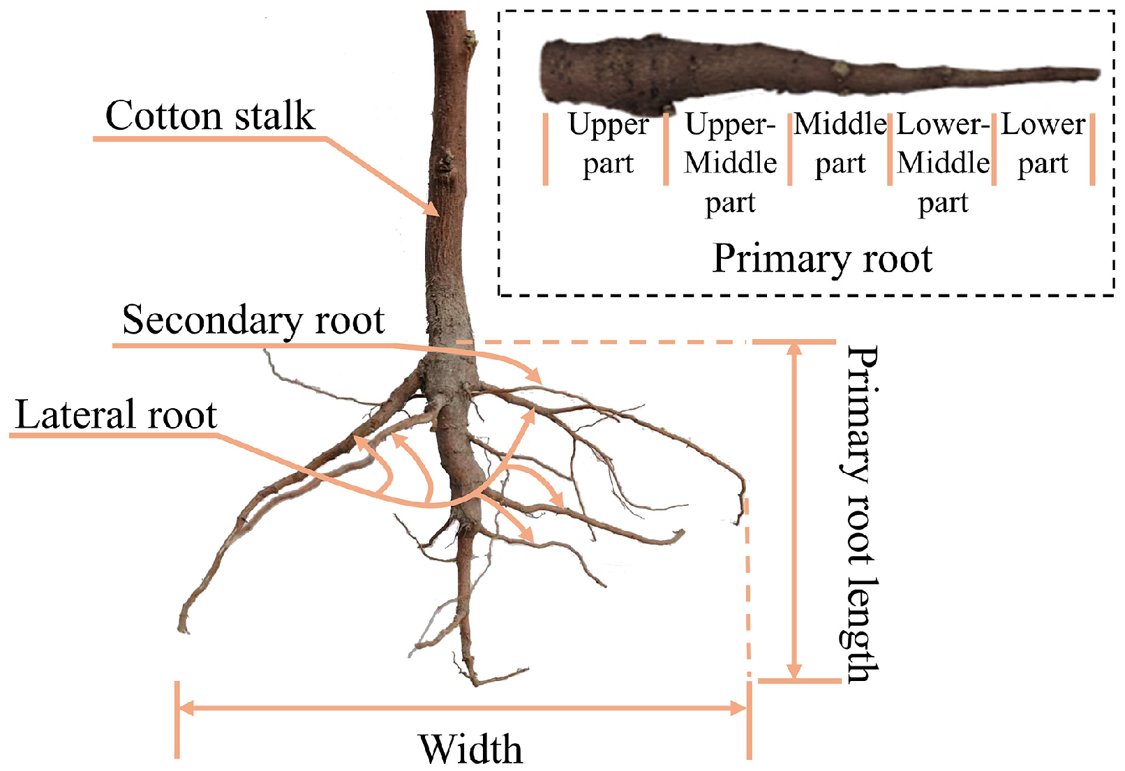
Figure 1. Morphology and structure of the cotton root system.
Agriculture 15 01827 g001
Figure 2. Measuring the friction coefficient: (a) test setup; (b) measurement schematic.
Agriculture 15 01827 g002
Figure 3. Measuring the restitution coefficient: (a) test setup; (b) keyframe of the highest point of rebound of the primary roots specimen; (c) keyframe of the highest point of rebound of the lateral roots specimen.
Agriculture 15 01827 g003
Figure 4. Image processing of the cotton roots stacking angle test: (a) original image; (b) grayscale image; (c) binarization process; (d) edge extraction; (e) fitting curve.
Agriculture 15 01827 g004
Figure 5. Shear test results: (a) primary roots shear test results; (b) lateral roots shear force-time curve.
Agriculture 15 01827 g005
Figure 6. Hertz–Mindlin with bonding contact model and its bonding bonds.
Agriculture 15 01827 g006
Figure 7. Discrete elemental modeling of cotton roots: (a) 3D scanner; (b) cotton roots (c) 3D model; (d) discrete element model.
Agriculture 15 01827 g007
Figure 8. A simulation model for the cotton roots stacking angle.
Agriculture 15 01827 g008
Figure 9. Shear simulation model.
Agriculture 15 01827 g009
Figure 10. Pareto chart of the Plackett–Burman test.
Agriculture 15 01827 g010
Figure 11. Interaction factors on the model stacking angle response surface: (a) response surface of interaction between X2 and X3; (b) response surface of interaction between X2 and X5; (c) response surface of interaction between X3 and X5.
Agriculture 15 01827 g011
Figure 12. Shear failure verification test: (a) actual shear test; (b) various stages diagrams of the bond fracture.
Agriculture 15 01827 g012
Figure 13. Tensile verification test: (a) actual tensile test; (b) actual image after root breakage; (c) initial stress on the root; (d) localized fracture in the root; (e) complete fracture of the root cross-section.
Agriculture 15 01827 g013
Figure 14. Tensile force evolution plots of both the actual tensile test on various samples and the simulation test.
Agriculture 15 01827 g014
Figure 15. Conducting field pull-up test: (a) trial cotton plots; (b) measuring the pull-up force.
Agriculture 15 01827 g015
Figure 16. Measuring the soil parameters in test fields: (a) determination of the moisture content; (b) determination of the firmness; (c) soil particle size screening.
Agriculture 15 01827 g016
Figure 17. Modeling the cotton root–soil composite.
Agriculture 15 01827 g017
Table 1. Structural dimensions of cotton root system.
ParametersValueNote
Primary rootUpper average diameter (mm)11.26Segment length 27.83 mm
Upper-middle average diameter (mm)9.12Segment length 23.57 mm
Middle average diameter (mm)7.24Segment length 22.61 mm
Lower-middle average diameter (mm)5.72Segment length 24.73 mm
Lower average diameter (mm)3.98Segment length 25.61 mm
Average length (mm)124.34
Lateral rootAverage diameter (mm)3.16
Average length (mm)68.44
Average quantity (mm)6.3
Root branching order2
Average branching angle (°)60
Average width (mm)126.8
Table 2. Cotton roots and steel plate intrinsic parameters.
ParametersPrimary RootsLateral RootsSteel
Density (kg·m−3)8858617850
Poisson’s ratio0.370.410.30
Shear modulus (Pa)6.93 × 1085.27 × 1067.94 × 1010
Table 3. Range values of cotton root contact parameters.
Simulation ParametersSymbolLow Level (−1)High Level (+1)
Restitution coefficient of root–rootX10.2390.428
Static friction coefficient of root–rootX20.4810.702
Rolling friction coefficient of root–rootX30.0500.250
Restitution coefficient of root–steelX40.4290.612
Static friction coefficient of root–steelX50.5630.616
Rolling friction coefficient of root–steelX60.0500.085
Table 4. Range of values for bonding parameters.
Simulation ParameterSymbolLow Level (−1)High Level (+1)
Normal stiffness per unit area of cotton root (N·m−3)X72.50 × 10104.15 × 1010
Shear stiffness per unit area of cotton root (N·m−3)X83.0 × 10105.6 × 1010
Critical normal stress of cotton root (MPa)X91040
Critical shear stress of cotton root (MPa)X101050
Table 5. CCD response surface experiment factor coding.
CodingX7 (N·m−3)X8 (N·m−3)X9 (MPa)X10 (MPa)
−22.5 × 10103.0 × 10101010
−12.91 × 10103.65 × 101017.520
03.33 × 10104.3 × 10102530
13.74 × 10104.95 × 101032.540
24.15 × 10105.6 × 10104050
Table 6. Plackett–Burman test design and results.
Serial No.Factorsθ′ (°)
X1X2X3X4X5X6
1−1−1−11−1121.51°
21−1−1−11−124.63°
31−111−1125.41°
4111−1−1−125.74°
511−1−1−1124.85°
6−1−1−1−1−1−123.13°
7−11−111−125.83°
811−111125.73°
9−1111−1−126.03°
101−1111−126.86°
11−1−11−11126.94°
12−111−11130.53°
Table 7. Plackett Burman experimental variance analysis.
ParametersStandardized EffectsSum of SquaresF-Valuep-ValueSignificance Ranking
X1−0.1250.04690.05310.82696
X21.7058.729.880.02563
X32.63820.8823.650.00461
X4−0.7421.651.870.22994
X52.30815.9918.100.00812
X60.4580.63020.71370.43685
Table 8. The steepest ascent test design and results.
Serial No.X2X3X5θ′ (°)φ (%)
10.4810.050.56322.31°16.16%
20.5360.100.57724.71°7.14%
30.5920.150.59025.52°4.10%
40.6470.200.60328.18°5.90%
50.7020.250.61629.55°11.05%
Table 9. Box–Behnken test design and results.
Serial No.Factorsθ′ (°)
X2X3X5
1−10−124.55
21−1024.12
301130.23
411028.51
500026.91
60−1−123.35
7−11026.99
800027.12
900026.84
1010128.58
1110−125.77
120−1125.75
1300026.44
14−10127.76
1501−126.65
1600026.69
17−1−1023.60
Table 10. Variance analysis of the Box–Behnken test.
ParametersDegree of FreedomMean SquareF-Valuep-ValueSignificance
Model95.94161.13<0.0001**
X212.0856.460.0001**
X3130.26821.12<0.0001**
X5118.00488.37<0.0001**
X2X310.256.780.0352*
X2X510.041.090.3322
X3X510.34819.440.0180*
X 2 2 10.716419.440.0031**
X 3 2 11.4338.760.0004**
X 5 2 10.32428.800.0209*
Residual70.0369
Lack of fit30.0001 0.9070
Pure error40.0644
Total16
** highly significant factor (p ≤ 0.01), * significant factor (p ≤ 0.05).
Table 11. The experimental design and results of the CCD response surface.
Serial No.FactorsFmax (N)
X7X8X9X10
11−111480.66
2−111−1442.38
31−1−1−1479.18
41−11−1476.77
50200468.53
6−11−11443.10
7−1111443.97
80−200440.64
90000466.85
10−1−1−11434.61
1111−11492.55
1211−1−1491.67
13−1−111433.39
14−2000416.03
150020468.29
160002468.41
1700−20466.87
18111−1490.83
19−1−1−1−1437.75
20−11−1−1442.05
21000−2470.43
22−1−11−1435.60
230000467.76
241111496.57
251−1−11479.58
262000505.12
270000466.76
Table 12. CCD response surface analysis of variance.
ParametersDegree of FreedomMean SquareF-Valuep-Value
Model14998.73345.44<0.0001
X7112,748.494409.46<0.0001
X81832.61287.98<0.0001
X910.26460.09150.7674
X1010.72110.24940.6265
X7X8139.9413.820.0029
X7X911.010.34930.5654
X7X10111.594.010.0684
X8X915.151.780.2066
X8X1016.662.300.1551
X9X1016.032.080.1744
X 7 2 163.1321.830.0005
X 8 2 1220.8876.40<0.0001
X 9 2 10.02060.00710.9342
X 10 2 15.141.780.2070
Residual122.89
Lack of fit103.4111.140.0852
Pure error20.3060
Total26
Table 13. Input parameters of the DEM developed for soil and its adjacent medium.
TypeParameterValueUnite
SoilPoisson’s ratio0.36
Shear modulus1.3 × 106Pa
Density1250kg·m−3
Soil–soilRestitution coefficient0.48
Static friction coefficient0.45
Rolling friction coefficient0.24
Normal stiffness per unit area1.15 × 108N·m−3
Shear stiffness per unit area3.06 × 108N·m−3
Critical normal stress6.9 × 105Pa
Critical shear stress6.7 × 105Pa
Soil–cotton rootsRestitution coefficient0.45
Static friction coefficient0.62
Rolling friction coefficient0.70
Bond stiffness 6.97 × 10⁶N·m−3
Bond stress 2.13 × 10⁶Pa
Bond radius1.39mm
Disclaimer/Publisher’s Note: The statements, opinions and data contained in all publications are solely those of the individual author(s) and contributor(s) and not of MDPI and/or the editor(s). MDPI and/or the editor(s) disclaim responsibility for any injury to people or property resulting from any ideas, methods, instructions or products referred to in the content.