Article

Optimization of Cotton Field Irrigation Scheduling Using the AquaCrop Model Assimilated with UAV Remote Sensing and Particle Swarm Optimization

1
College of Hydraulic and Civil Engineering, Xinjiang Agricultural University, Urumgi 830052, China
2
Xinjiang Future Irrigation District Engineering Technology Research Center, Wensu 843100, China
3
College of Water Engineering, Yellow River Conservancy Technical University, Kaifeng 475000, China
4
School of Science, Xi’an University of Technology, Xi’an 710054, China
5
State Key Laboratory of Eco-Hydraulics in Northwest Arid Region, Xi’an University of Technology, Xi’an 710048, China
*
Authors to whom correspondence should be addressed.
Agriculture 2025, 15(17), 1815; https://doi.org/10.3390/agriculture15171815
Submission received: 17 July 2025 / Revised: 18 August 2025 / Accepted: 22 August 2025 / Published: 26 August 2025
(This article belongs to the Section Agricultural Water Management)

Abstract

In arid and semi-arid agricultural regions, the increasing frequency of extreme climatic events—particularly high temperatures and drought—has severely disrupted crop growth dynamics, leading to significant yield uncertainty and potential threats to the growing global food demand. Optimizing irrigation strategies by integrating dynamic crop growth monitoring and accurate yield estimation is essential for mitigating the adverse effects of extreme weather and promoting sustainable agricultural development. Therefore, this study conducted two consecutive years of field experiments in cotton fields to evaluate the effects of irrigation interval and drip irrigation frequency on cotton growth dynamics and yield, and to develop an optimized irrigation schedule based on the AquaCrop model assimilated with Particle Swarm Optimization (AquaCrop-PSO). The sensitivity analysis identified the canopy growth coefficient (CGC), maximum canopy cover (CCX), and canopy cover at 90% emergence (CCS) as the most influential parameters for canopy cover (CC) simulation, while the crop coefficient at full canopy (KCTRX), water productivity (WP), and CGC were most sensitive for aboveground biomass (AGB) simulation. Ridge regression models integrating multiple vegetation indices outperformed single-index models in estimating CC and AGB across different growth stages, achieving R2 values of 0.73 and 0.87, respectively. Assimilating both CC and AGB as dual-state variables significantly improved the model’s predictive accuracy for cotton yield, with R2 values of 0.96 and 0.95 in 2023 and 2024, respectively. Scenario simulations revealed that the optimal irrigation quotas for dry, normal, and wet years were 520 mm, 420 mm, and 420 mm, respectively, with a consistent irrigation interval of five days. This study provides theoretical insights and practical guidance for irrigation scheduling, yield prediction, and smart irrigation management in drip-irrigated cotton fields in Xinjiang, China.

1. Introduction

Recent developments in precision agriculture and intelligent crop management have heightened the demand for improved simulation accuracy and broader applicability of crop growth models [1]. However, traditional crop models often struggle to accurately capture temporal and spatial variations in field crops due to uncertain input parameters and delayed responses to environmental changes [2]. In contrast, remote sensing technology, which offers extensive and frequent observation data with excellent real-time and spatial coverage, can be integrated with traditional crop models to enhance dynamic monitoring outcomes [3]. Consequently, effective assimilation of remote sensing data into crop models cannot only dynamically reflect intrinsic crop growth mechanisms but also enable real-time crop growth monitoring, significantly improving model accuracy and practicality [4].
Currently, methods for assimilating remote sensing data with crop models primarily include forcing, sequential assimilation, and parameter optimization. The forcing method directly replaces certain state variables within the model with observations derived from remote sensing, commonly substituting leaf area index (LAI) inputs; however, its accuracy depends heavily on the timeliness and precision of remote sensing data [5,6]. Sequential assimilation, also known as the updating method, continuously corrects the model state using remote sensing observations, typically employing techniques such as Kalman Filtering (KF) [7], Ensemble Kalman Filtering (EnKF) [8], and variational assimilation methods [9]. Parameter optimization methods minimize systematic biases between simulations and remote sensing observations by constructing cost functions and optimizing model parameters. Common algorithms in this category include Particle Swarm Optimization (PSO) [10,11] and Simulated Annealing (SA) [12].
Unmanned aerial vehicles (UAVs) have emerged as a flexible, cost-effective, and high-resolution platform for acquiring multispectral or thermal imagery, enabling timely monitoring of crop growth dynamics at the field scale. Compared with satellite remote sensing, UAV-based observations offer finer spatial resolution and higher revisit frequency, making them particularly suitable for precision agriculture. However, their integration into crop growth models such as AquaCrop remains relatively underexplored, especially in arid and semi-arid agricultural regions. Recent studies have shown the benefits of assimilating remotely sensed canopy cover (CC) into crop models to improve parameter estimation and yield predictions. For example, Dalla Marta et al. [13] integrated Sentinel-2-derived CC into AquaCrop for tomato water requirement assessment in southern Italy, demonstrating significant improvements in irrigation scheduling. Upreti et al. [14] applied Bayesian calibration to AquaCrop-OS using high-resolution CC data, reducing parameter uncertainty for durum wheat. Yokoyama et al. [15] assimilated UAV-derived leaf area index (LAI) into the WOFOST model to predict cabbage yield at the plant level, illustrating the high potential of UAV observations for improving crop model robustness.
In this study, we developed a novel integration framework that couples UAV-based remote sensing with the AquaCrop model through Particle Swarm Optimization (PSO) for parameter assimilation. The novelty of this approach lies in leveraging PSO’s global search capability in high-dimensional nonlinear optimization to systematically calibrate key crop parameters while maintaining the physical consistency of the AquaCrop model. Unlike conventional methods that directly replace state variables or assume specific observational error distributions, our framework seamlessly assimilates remotely sensed canopy cover (CC) and aboveground biomass (AGB) data without compromising model structure. This innovation not only improves simulation accuracy and stability but also enhances the dynamic prediction of cotton yield. Moreover, it provides a scalable and transferable methodology for optimizing irrigation scheduling, offering valuable theoretical and technical support for precision agriculture in arid and semi-arid regions.
Existing research on assimilating remote sensing data with crop models mainly focuses on satellite or hyperspectral remote sensing. Studies demonstrate that integrating remote sensing data significantly enhances crop yield simulation accuracy [16,17,18]. For instance, Francesco Novelli et al. [19] assimilated satellite-derived leaf area index (LAI) into the Environmental Policy Integrated Climate model (EPIC) model, considerably reducing discrepancies between observed and simulated LAI, thereby significantly improving crop yield estimations. Similarly, Junyi Liu et al. [20] combined the WOrld FOod STudies model (WOFOST) crop growth model with Sentinel-2 satellite data, enhancing model adaptability to specific parameters and spatiotemporal representativeness of LAI observations, thus effectively estimating maize hybrid yield. Sellaperumal Pazhanivelan et al. [21] calibrated the Decision Support System for Agrotechnology Transfer (DSSAT) model using remote sensing data, enhancing the model’s capability to capture physiological responses of rice and consequently improving regional rice yield simulation accuracy.
It is noteworthy that existing studies often assimilate single crop parameters (e.g., LAI) without fully exploring the potential of multi-parameter assimilation [22,23]. Chunyan Ma [24] and Curenl [25] demonstrated significant improvements in wheat yield estimation accuracy by assimilating LAI derived from multi-source satellite imagery. However, studies utilizing unmanned aerial vehicle (UAV) remote sensing data for assimilation into crop models remain limited, especially concerning the AquaCrop model. AquaCrop, developed by the FAO, is specifically designed to simulate the relationship between water availability and crop yield with relatively few parameters and modest data requirements, making it particularly suitable for water-limited environments and precision irrigation scheduling. In contrast, the DSSAT model requires a large number of crop, soil, and management parameters and is often calibrated using extensive field experiments, while the WOFOST model emphasizes detailed physiological process simulation and has relatively high data demands, which can limit their rapid application in data-scarce regions. UAV-derived observations offer unique advantages for AquaCrop assimilation by providing ultra-high spatial resolution, flexible revisit capability, and timely measurements of key crop variables such as canopy cover (CC) and aboveground biomass (AGB). These features enable the capture of within-field heterogeneity and rapid responses to environmental or management changes, thereby enhancing the performance of AquaCrop assimilation and improving its predictive accuracy and applicability for irrigation scheduling optimization.
Therefore, this study focused on cotton cultivation at the Huaxing Farm in Changji Hui Autonomous Prefecture, Xinjiang, China. Using field experiment data from 2023 and 2024, the Extended Fourier Amplitude Sensitivity Test (EFAST) identified critical AquaCrop parameters. A PSO-based assimilation strategy was developed to optimize the dual-state variables of CC and AGB, ultimately constructing the AquaCrop-PSO model. The model’s simulation accuracy under various irrigation scenarios was assessed, and its application potential in optimizing irrigation scheduling and predicting seed cotton yield was explored. The outcomes provide theoretical support and a technological framework for smart irrigation management in arid-region cotton fields, with three specific objectives: (1) model improvement—to enhance the accuracy of crop growth simulation by assimilating UAV-derived canopy cover (CC) and aboveground biomass (AGB) into the AquaCrop model using a multi-variable assimilation framework; (2) yield prediction—to evaluate the capability of the improved AquaCrop model in predicting seed cotton yield under different irrigation scenarios; and (3) irrigation optimization—to determine optimal irrigation scheduling strategies for water-limited environments by coupling the improved AquaCrop model with the PSO algorithm.

2. Materials and Methods

2.1. Experimental Site Description

The field experiments were conducted from April to October in 2023 and 2024 at the Huaxing Farm experimental base in Daxiqu Town, Changji City, Xinjiang Uygur Autonomous Region, China (87°30′38″ E, 44°21′59″ N). The location of the experimental area and layout of plots are shown in Figure 1. The experimental site’s soil texture is clay loam, containing organic matter of 12.90 g·kg−1, available phosphorus of 35.65 mg·kg−1, rapidly available potassium of 479.5 mg·kg−1, hydrolyzable nitrogen of 27.49 mg·kg−1, total nitrogen of 0.67 g·kg−1, water-soluble salts of 4.50 g·kg−1, soil bulk density of 1.49 g·cm−3, and field water holding capacity of 22% (volumetric water content). This value represents the average field water holding capacity, determined through field sampling using the ring knife method based on undisturbed soil cores collected from the 0–60 cm soil profile.

2.2. Cotton Irrigation Experiment Design and Crop Management

The experiment employed subsurface drip irrigation with cotton variety Zhongmian 113, planted using a “one-film-three-tubes-six-rows” mechanically harvested cotton planting pattern, featuring row spacing of 66 + 10 cm and plant spacing of 8.5 cm. Drip irrigation tapes were placed at the center of the narrow rows, with emitter flow rates of 2.6 L·h−1 and emitter spacing of 25 cm. Irrigation water was sourced from a channel system, with precise irrigation volumes controlled via water meters. To align the experimental conditions with standard production practices, no special soil amendments or fertilization treatments were applied before sowing, and fertilization protocols followed the local standardized cultivation guidelines. Cotton was sown on 23 April 2023 and 28 April 2024 and harvested on 5 October 2023 and 30 September 2024. Experimental data collection periods were from 8 June to 5 October 2023 and from 8 June to 30 September 2024. The experimental design included various combinations of irrigation cycles and frequencies, with specific treatments and plot layouts detailed in Table 1. Each treatment was conducted with three replicates, and the plots were arranged in a randomized complete block design to minimize the effects of spatial heterogeneity.

2.3. Data Collection

2.3.1. UAV-Based Remote Sensing Data Acquisition and Processing

In this study, vehicle (UAV) remote sensing imagery was acquired using a Matrice 350 RTk UAV (DJI Innovations, Shenzhen, China). equipped with a RedEdge-P multispectral camera at different growth stages of cotton. The RedEdge-P camera features five narrow spectral bands (see Table 2), suitable for vegetation parameter inversion and monitoring. A total of 15 flight missions were conducted during the 2023 and 2024 growing seasons, covering key phenological stages including seedling, squaring, flowering, boll-setting, and boll-opening. All flights were carried out under clear, cloud-free weather conditions, with flight altitudes set at 30 m and altitude control managed by an RTK positioning system. Radiometric calibration was performed by capturing images of a gray calibration board before each flight. Flights were consistently scheduled between 13:00 and 14:00 to ensure stable illumination conditions. During image acquisition, the camera lens was oriented vertically downward to capture multispectral imagery of the cotton canopy.
Due to atmospheric heterogeneity and sensor-related distortions, multispectral imagery acquired by UAVs typically requires preprocessing [26]. Pix4Dmapper 4.7 software was used for radiometric correction, image registration, and mosaic stitching of the raw images. Geometric correction and regional cropping were conducted using ArcGIS 10.7 software. High-precision geometric corrections were performed by matching RTK-acquired high-precision ground control points with corresponding points in the mosaicked images. To ensure spatial and pixel consistency across all spectral bands, multispectral images were uniformly cropped to exclude non-study areas, ensuring identical image dimensions and coordinates before reflectance analysis.

2.3.2. Leaf Area Index (LAI) Measurement

At each cotton growth stage, the leaf area index (LAI) was measured for each irrigation treatment using a randomized sampling approach. UAV remote sensing data were simultaneously acquired during field measurements to ensure consistency in growth monitoring. LAI measurements were performed using the punch-and-weigh method, in which nine cotton plants were randomly selected per treatment plot [27]. The average of these nine plants was taken as the representative LAI value for that treatment. The measured LAI was then used to estimate canopy cover (CC) using the following equation:
C C = 1 e x p ( L A I 3 ) 1 + e x p ( L A I 3 )
L A I = t h e   l e a f   a r e a t h e   g r o u n d   a r e a   o c c u p i e d

2.3.3. Biomass and Yield Measurement

At each cotton growth stage, destructive sampling was conducted using a randomized approach. Sampled cotton plants were rinsed and blotted dry using absorbent paper. The plants were then separated into stems, leaves, and reproductive organs (flowers and bolls) using pruning shears. Samples were first inactivated at 105 °C and then oven-dried at 75 °C to a constant weight. The dry weights of stems, leaves, and reproductive parts were measured with a precision of 0.01 g.
At harvest, three 6.67 m2 quadrats were randomly selected in each experimental plot for manual harvesting. The collected seed cotton was air-dried to a constant weight, and the final yield was determined gravimetrically.

2.3.4. Vegetation Index (VI) Calculation

Vegetation indices (VIs) are derived from multispectral information and are useful for evaluating crop growth [28]. By mathematically combining spectral bands, VIs reduce the influence of atmospheric reflections at different times on multispectral sensors, thus accelerating data acquisition and expanding coverage areas. Currently, vegetation indices are extensively employed to monitor plant phenotypic data, track crop growth progression, and assess ecological conditions. Although traditional methods extract vegetation indices by analyzing reflectance from specific spectral bands, relying solely on a single band can obscure significant spectral features (e.g., green or red), potentially causing false interpretations such as “false greenness” or “false redness”. [29] Therefore, multi-angle and multi-level extraction and analysis of spectral features are particularly critical. For instance, vegetation indices calculated using red, blue, and near-infrared bands effectively monitor vegetation canopy growth. VIs integrate the reflective and absorptive characteristics of healthy green vegetation across different bands, mathematically processing this multiband reflectance data to enhance vegetation information representation. In this study, 22 vegetation indices were calculated based on cotton canopy reflectance data. The calculation formulas and specific band combinations for these indices are detailed in Appendix A

2.3.5. Meteorological Data Collection

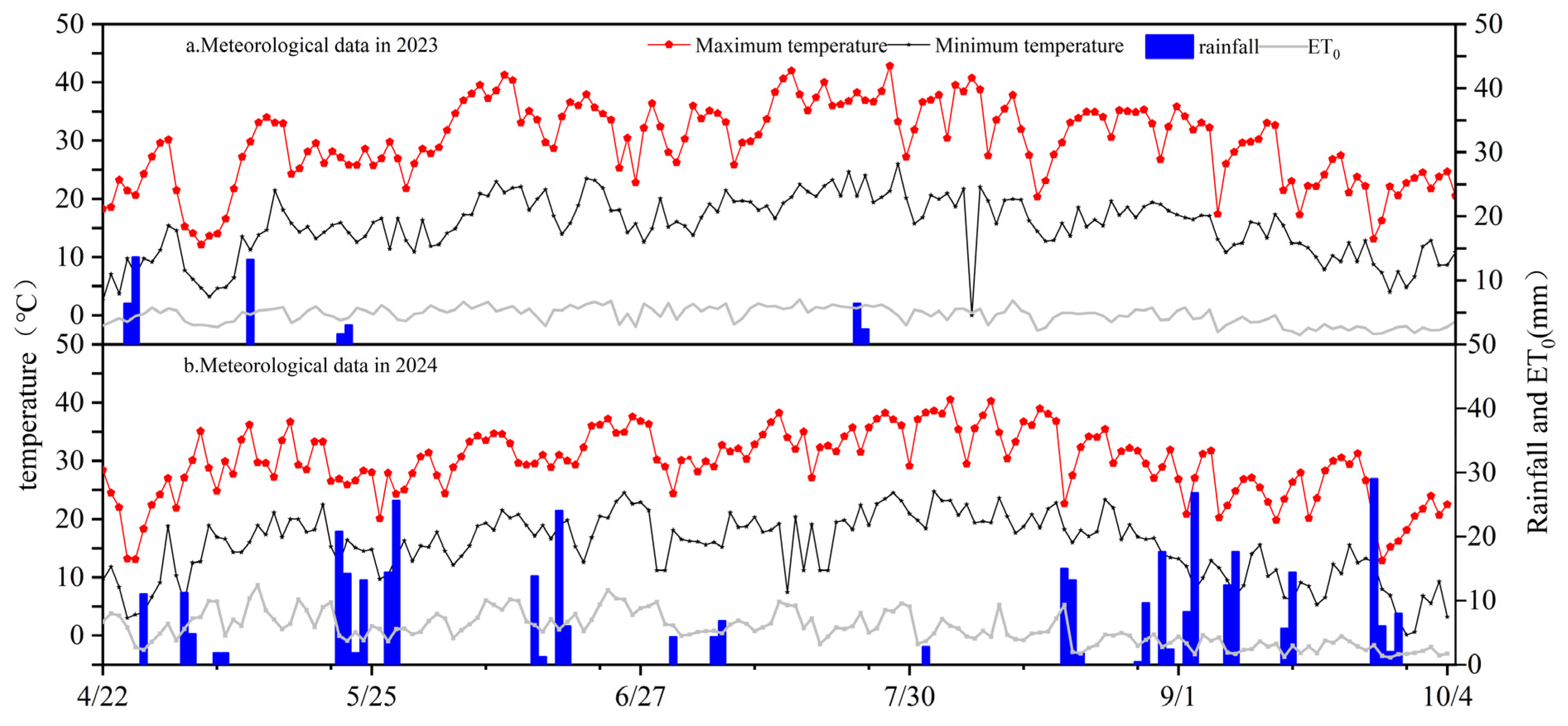
Meteorological data used in this study were obtained from the automatic weather station located at the Smart Agriculture Demonstration Zone of the Changji National Agricultural Science and Technology Park, approximately 5 km from the experimental site. The monitored parameters included air temperature (T), relative humidity (RH), wind speed (WS), net solar radiation (Rn), and precipitation (P), with data recorded every 30 min and automatically uploaded to a central data platform. Based on these meteorological observations, the reference evapotranspiration (ET0) was calculated using the FAO Penman–Monteith method [30]. Figure 2 illustrates the daily variations in precipitation, temperature, and reference crop evapotranspiration (ET0) during the cotton phenological stages from 2023 to 2024.

2.3.6. Fundamental Principles of the AquaCrop Model

The AquaCrop model, developed by the Food and Agriculture Organization of the United Nations (FAO) in 2009, is a process-based crop growth simulation model. Detailed descriptions of AquaCrop can be found in the works of Steduto, P. [31] and Jin, X.L. [32]. AquaCrop distinguishes evapotranspiration into two components: soil evaporation (E) and crop transpiration (Tr), thereby separating non-productive water use from productive water use. Final crop yield (Y) is partitioned into aboveground biomass (AGB) and harvest index (HI), enabling the model to differentiate the effects of water stress on AGB and HI. The core model equations are as follows:
Y = B × H I
B = W P × T r
In the equations, Y represents the crop yield (t·hm−2); B is the accumulated aboveground biomass (AGB) (t·hm−2); HI denotes the harvest index (%); WP is the water productivity of biomass production (kg·m−2·mm−1); and Tr is the crop transpiration (mm).
In the AquaCrop model, crop canopy development is simulated using canopy cover (CC, %) instead of the traditional leaf area index (LAI). Canopy cover over time is modeled based on the canopy growth coefficient (CGC) and is calculated using the following equation:
C C = C C 0 × e t × C G C ,                                                                               C C C C x 2 C C = C C x 0.25 C C x C C 0 × e ( t ) × C G C ,                       C C C C x 2
In the equation, CC represents the canopy cover at time t (where t is expressed in days or growing degree days, GDD); CC0 is the initial canopy cover at 90% seedling emergence (%); and CCx is the maximum canopy cover when the canopy is fully developed (%).
During the canopy senescence phase, the reduction in canopy cover is represented by the canopy decline coefficient (CDC), calculated as follows:
C C = C C x 1 0.05 ( e C D C C C x 1 )

2.3.7. Principle of Particle Swarm Optimization (PSO)

Particle Swarm Optimization (PSO) is a swarm intelligence-based optimization algorithm used to solve both continuous and discrete optimization problems. It is based on the concept of a particle swarm and transforms the global optimum into a local optimum through certain rules to achieve global optimization [33].
In this study, aboveground biomass (AGB) and canopy cover (CC) during the cotton growth process were used as state variables. Based on vehicle (UAV) remotely sensed AGB and CC values, the PSO data assimilation algorithm was coupled with the AquaCrop model to construct the AquaCrop-PSO assimilation model. During the assimilation process, sensitive crop parameters in the AquaCrop model were continuously adjusted. The model parameters were initialized, and a cost function was constructed based on the optimized simulated values of AGB and CC and their remotely sensed counterparts. The cost function was iteratively minimized until convergence. The calibrated parameters were then used as the initial input for the AquaCrop model, which was run to obtain the assimilated values of AGB, CC, and yield, thus realizing the assimilation of vehicle (UAV) remote sensing data information into the crop growth model.

2.3.8. Extended Fourier Amplitude Sensitivity Test

The Extended Fourier Amplitude Sensitivity Test (EFAST) is a variance-based method that combines the FAST method and the Sobol method, taking into account the nonlinear response of the mode [34]. The EFAST method generates two types of sensitivity indices: the first-order sensitivity index Si, which describes the effect of a single parameter variation on the model output; and the total sensitivity index STi, which describes the influence of parameter interactions on the model output. Both Si and STi range between 0 and 1, and higher values indicate that the input parameter is more sensitive to the output variable. In this study, Si > 0.05 and STi > 0.1 were used as the criteria for identifying sensitive parameters. The parameters that met these criteria were then selected as the decision variables for the subsequent PSO-based optimization, ensuring that the optimization process focused on the most influential factors affecting CC and AGB simulation accuracy.
The equations for calculating the first-order sensitivity index Si and the total sensitivity index STi are as follows:
S i = V i V ( Y )
S T i = V Y V i V Y
In the equations, V (Y) is the output result; Vi is the model variance caused by the individual variation of input parameter xi; and V−i is the variance of all parameters except for the i-th parameter.
In this study, the EFAST method was used to perform sensitivity analysis on 26 parameters in the AquaCrop model, as listed in Appendix Table A2. The detailed steps of the sensitivity analysis are as follows:
(1) The initial values of crop parameters were based on the FAO Crop Parameter Manual. Then, each parameter was independently and uniformly varied within ±35% of its initial value.
(2) A Monte Carlo method was used to randomly sample the parameters. A total of 3800 samples were generated (EFAST recommends that the sample size should exceed 65 times the number of parameters for reliable results).
(3) A Python (version 3.10, 64-bit) script was developed to call the AquaCrop model plugin ACsaV70 for batch simulations (total number of simulations: 3800 × 26 × 3), and the output was collected.
(4) Sensitivity analysis was performed using Simlab software (version 2.2.1). Results from both years were averaged to obtain the final sensitivity indices.

2.4. Model Evaluation Metrics

To evaluate the model performance in this study, the coefficient of determination (R2) and root mean square error (RMSE) were used as statistical indicators of fitting accuracy. A higher value of R2 and d approaching 1, along with a lower RMSE value, indicate better model estimation accuracy.

3. Results and Discussion

3.1. Sensitivity of AquaCrop Model Parameters for Canopy Cover and Aboveground Biomass

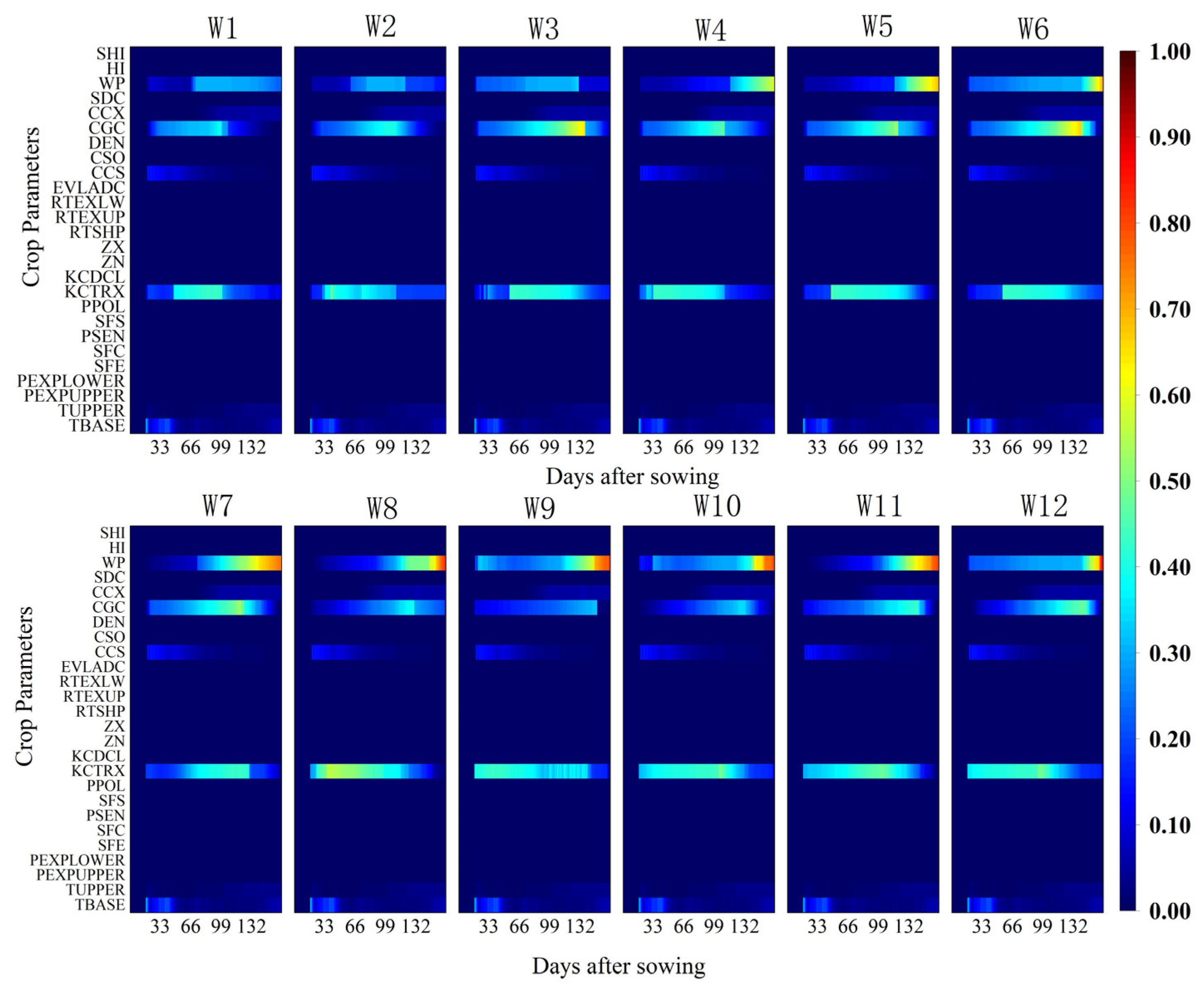
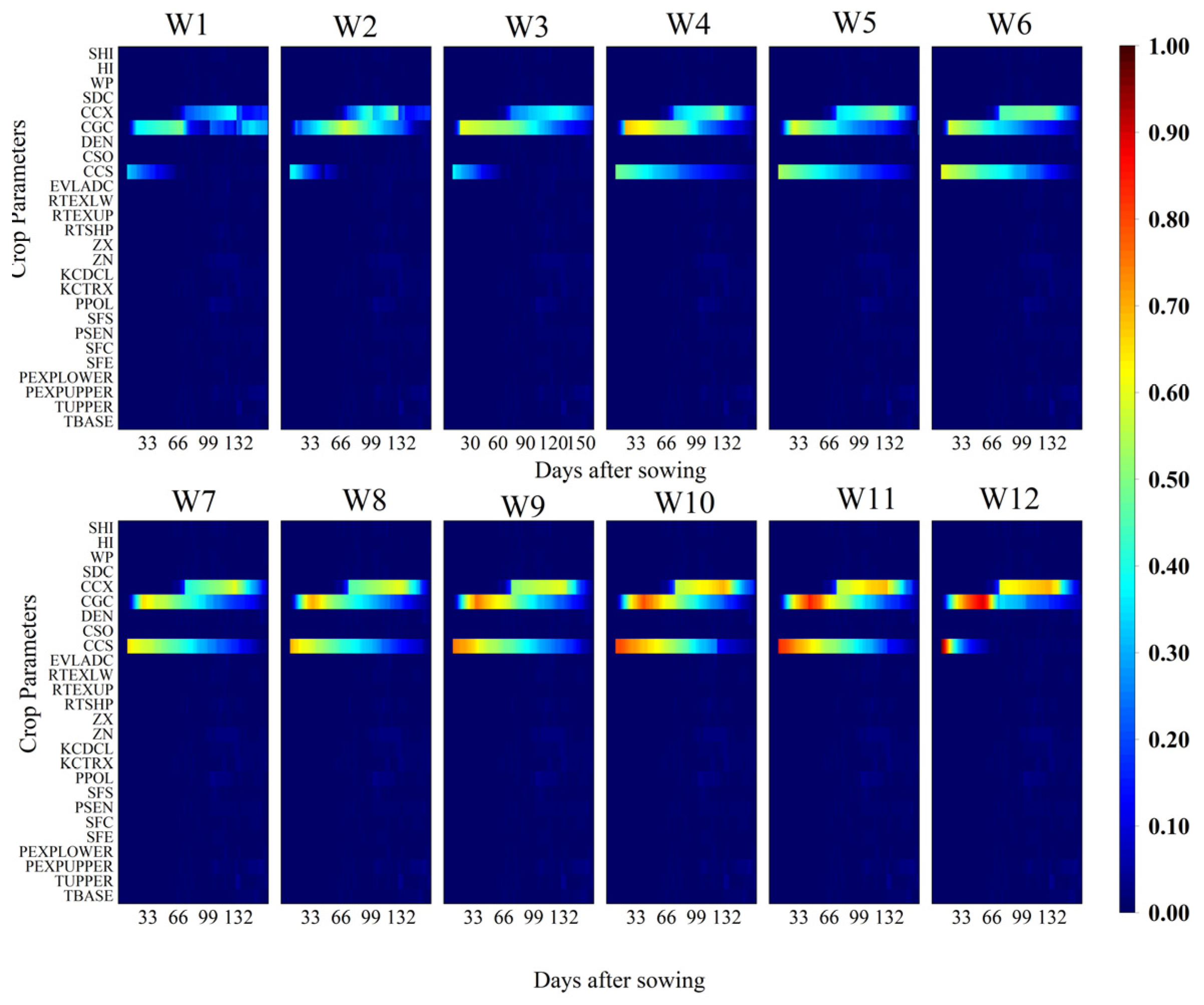
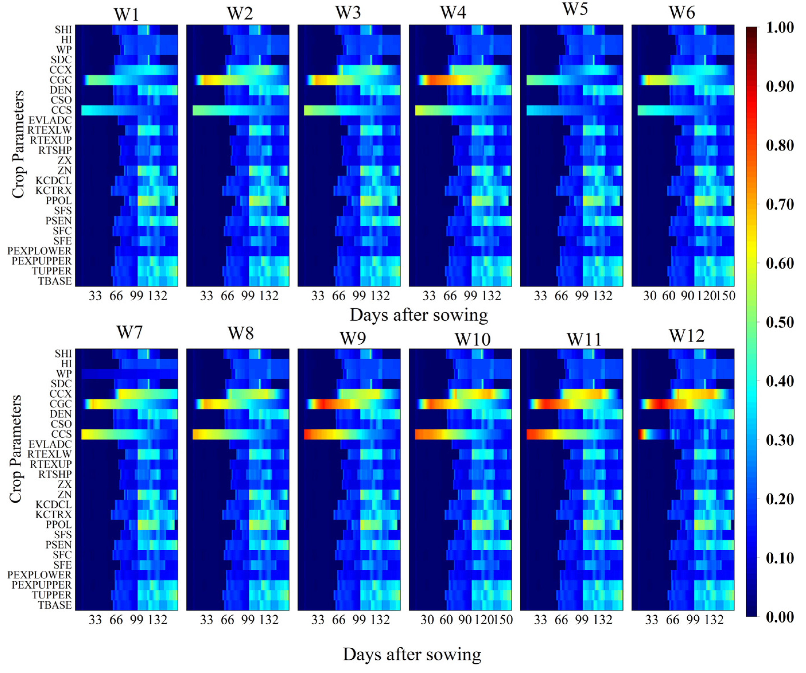
Figure 3 and Figure 4 illustrate the dynamic variations of the first-order sensitivity index (FOSI) and total-order sensitivity index (TOSI) of aboveground biomass (AGB) in response to key AquaCrop model parameters under twelve different irrigation treatments (W1–W12). The results indicate that the three most sensitive parameters for AGB were the crop coefficient at full canopy (KCTRX), water productivity (WP), and canopy growth coefficient (CGC), which correspond to key physiological processes in crop growth as represented in the AquaCrop model. Specifically, KCTRX reflects the crop’s transpiration capacity at full canopy and represents the regulation of stomatal conductance and CO2 assimilation efficiency, directly influencing the accumulation of photosynthetic products. WP measures the dry matter produced per unit of transpired water, integrating water use efficiency and carbon fixation capacity. CGC controls the canopy expansion rate, determining the light interception area and potential transpiration surface during early growth stages. These three parameters jointly regulate AGB formation from different dimensions, including photosynthetic structure development, gas exchange efficiency, and water-to-biomass conversion effectiveness. Among these, FOSI values for KCTRX exhibited a “rise-then-decline” trend over time across irrigation treatments. Furthermore, the timing of peak sensitivity shifted later with increased irrigation quotas. The sensitivity index of WP increased significantly starting from the 66th day after sowing and peaked during the late growth stages, indicating its substantial impact on biomass accumulation during this period. The sensitivity of CGC intensified with greater irrigation quotas and shorter irrigation intervals, indicating prolonged influence on AGB.
Additionally, CCS (canopy cover at 90% emergence) and TBASE (base temperature) also showed sensitivity to AGB during the emergence to flowering stages. The TOSI results (Figure 4) confirmed the dominant influence of KCTRX, WP, and CGC on AGB, verifying the consistency and robustness of the FOSI analysis. These findings suggest that AGB formation in the model is primarily governed by the interaction between WP, crop transpiration (Tr), and reference evapotranspiration (ET0), with KCTRX indirectly influencing AGB via Tr, and CGC affecting biomass accumulation through its impact on canopy expansion.
Figure 5 and Figure 6 present the parameter sensitivity of canopy cover (CC) under different irrigation treatments. The analysis revealed that CGC, maximum canopy cover (CCX), and CCS were the principal parameters influencing CC. CGC exhibited high sensitivity between 20 and 96 days after sowing, coinciding with the rapid canopy expansion phase. Sensitivity to CCX began to increase on day 56 after sowing and intensified with increasing irrigation quotas and prolonged irrigation intervals. CCS exerted a stronger influence on CC during the early growth stages, with its sensitivity gradually declining as the crop developed.
Overall, the sensitivity of AGB and CC to model parameters showed stage-specific responses. Under high-frequency and high-quota irrigation conditions, sensitive parameters exerted a more prolonged influence on model outputs. These findings provide theoretical support for subsequent parameter optimization and assimilation of vehicle (UAV) remote sensing data variables into the AquaCrop model.

3.2. UAV Remote Sensing Inversion of Aboveground Biomass and Canopy Cover

3.2.1. Correlation Between Vegetation Indices and Aboveground Biomass (AGB) and Canopy Cover (CC)

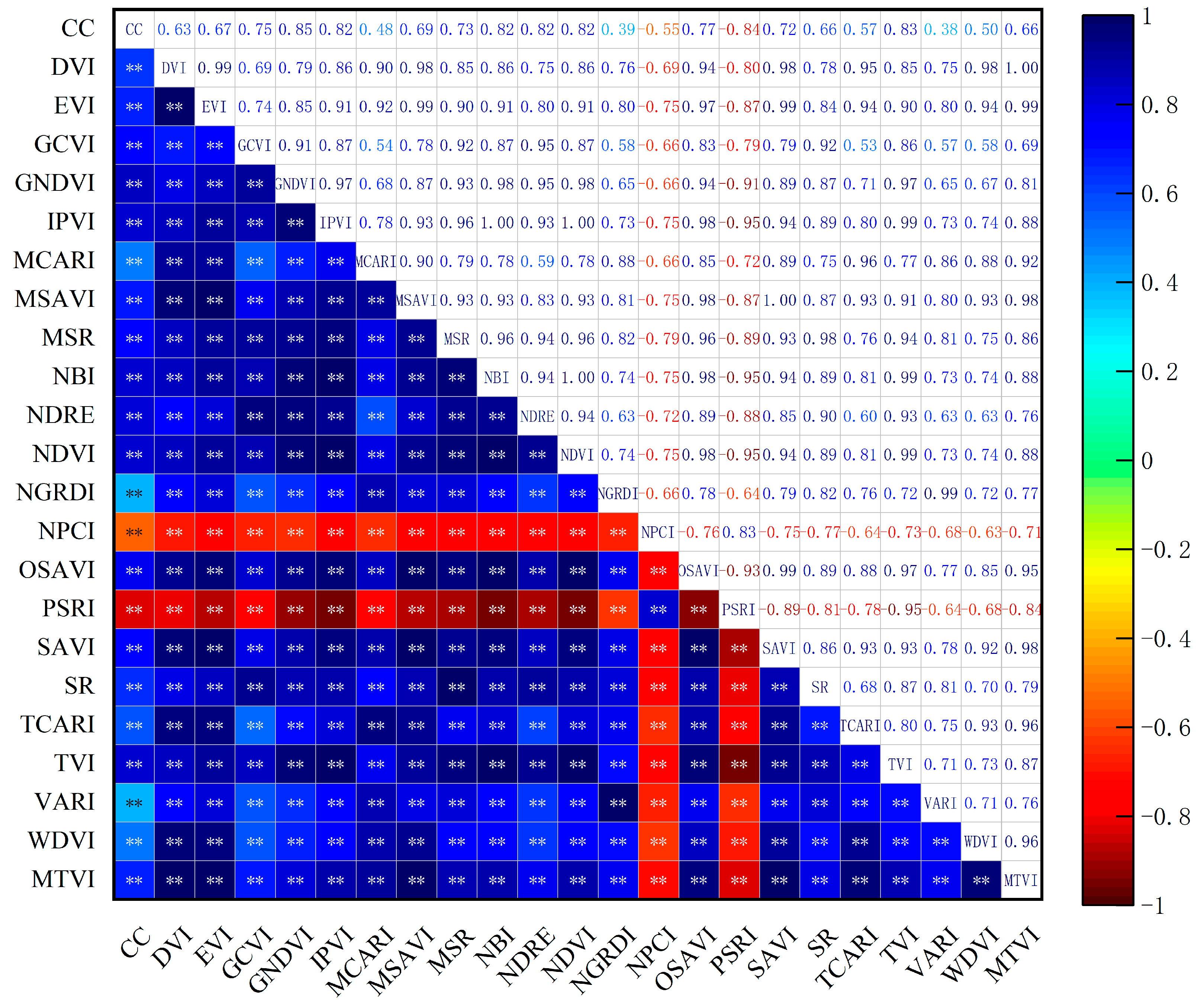
To identify the most suitable vegetation indices (VIs) for UAV remote sensing inversion of cotton growth, this study evaluated the relationships between various VIs and measured canopy cover (CC) and aboveground biomass (AGB) across different growth stages. For AGB, a gray relational analysis was conducted prior to modeling, while Pearson correlation analysis was employed to assess the significance and fitting accuracy of VIs with respect to CC, The results are presented in Figure 7.
GNDVI exhibited the highest correlation with canopy cover (CC) (r = 0.85), highlighting its strong ability to characterize structural variations in the cotton canopy. In addition to GNDVI, other vegetation indices such as TVI, NDVI, NBI, NDRE, and IPVI also showed relatively high correlations (r = 0.82–0.83), indicating their effectiveness in reflecting canopy closure, leaf area development, and vegetation greenness. Comparable results have been reported by other researchers. Gordillo-Salinas et al. [35] found that UAV-derived GNDVI was highly correlated with aboveground biomass in wheat, with a coefficient of determination (R2) reaching 0.84, effectively capturing canopy development. Similarly, Lacerda et al. [36] identified GNDVI as the most suitable vegetation index for estimating cotton plant height, reporting correlation coefficients of 0.72 and 0.84 across two growing seasons. These findings collectively support the robustness of GNDVI and related indices in monitoring crop canopy traits. In contrast, NPCI and PSRI were negatively correlated with CC, with correlation coefficients of –0.54 and –0.83, respectively, likely due to their sensitivity to red or blue reflectance, which may interfere with the characterization of healthy canopy conditions.
For AGB, gray relational degrees between measured AGB and various vegetation indices were calculated at key phenological stages: seedling, budding, flowering, boll-setting, and boll-opening stages (Table 3). The results revealed pronounced stage-specific differences in the association between AGB and VIs. From budding to boll-setting stages, the relational degrees were notably higher, indicating that this period corresponds to rapid biomass accumulation and that VI dynamics effectively captured AGB variations.
At the seedling stage, PSRI, VARI, SR, NPCI, and DVI exhibited the highest correlation degrees with AGB, while MSR had the lowest (0.59). During the budding stage, PSRI, NPCI, VARI, GNDVI, and OSAVI showed the highest association, although MSR increased slightly to 0.69 but remained the lowest. In the flowering stage, VARI, TCARI, OSAVI, MSAVI, and EVI ranked highest in relational degree, while MSR dropped to 0.53. During the boll-setting stage, MTVI, VARI, EVI, TCARI, and MSAVI had the strongest associations, with MSR slightly improving to 0.66. In the boll-opening stage, the top indices included VARI, PSRI, NPCI, DVI, and WDVI, while SR showed the lowest correlation (0.45).
Overall, indices such as VARI, PSRI, and NPCI consistently demonstrated high sensitivity to AGB across multiple growth stages, making them suitable for multi-temporal AGB estimation in cotton fields. In contrast, MSR showed poor performance throughout all stages, possibly due to insufficient spectral sensitivity to canopy structural or photosynthetic variations arising from its formulation.

3.2.2. Construction of UAV Remote Sensing Inversion Models for Canopy Cover and Biomass

To further evaluate the applicability of combined vegetation indices in the inversion of cotton canopy cover (CC) and aboveground biomass (AGB), both univariate linear regression and multivariate ridge regression models were constructed and validated based on the correlation analysis results. The performance differences between univariate and multivariate models were systematically compared.
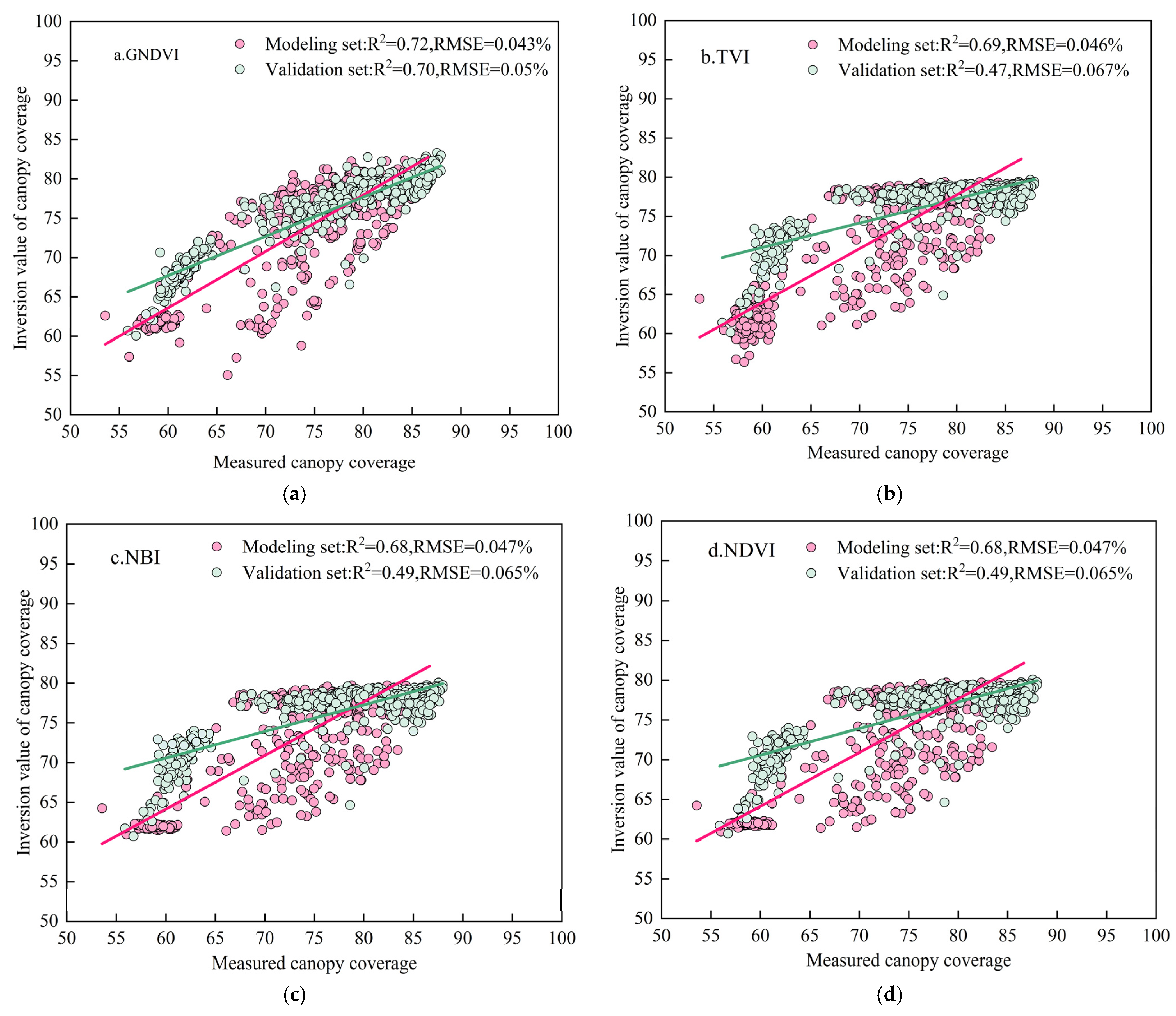
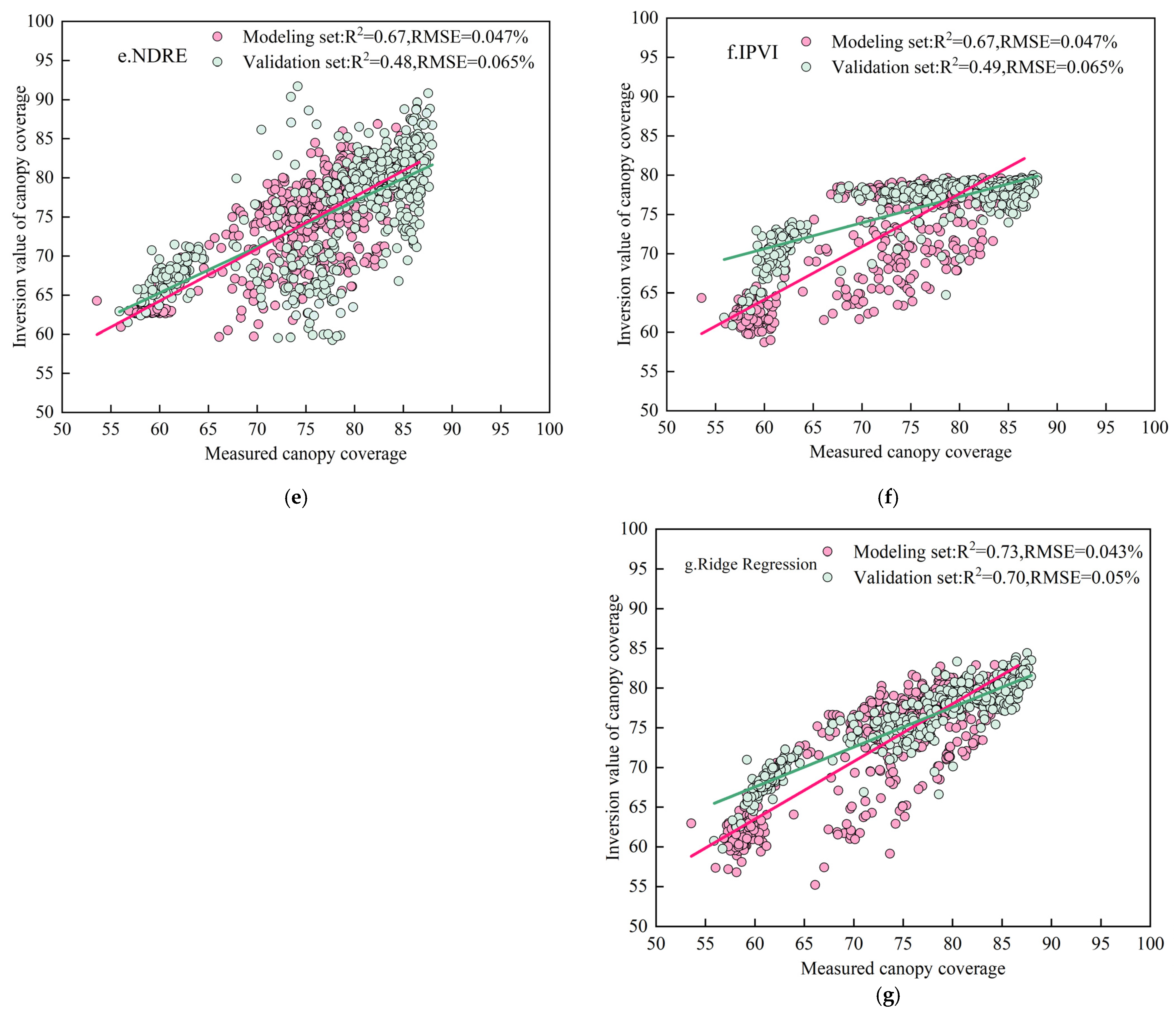
For CC estimation, the six vegetation indices with the highest correlation coefficients were selected to develop a ridge regression model. In addition, separate univariate linear regression models were built for each of these six indices. The dataset from 2023 (n = 540) was used for model training, while the dataset from 2024 (n = 540) was used for validation. The modeling and validation results are presented in Figure 8 and Table 4.
During the training phase, the univariate model based on GNDVI showed the best performance, with a coefficient of determination (R2) of 0.72 and a root mean square error (RMSE) of 0.043%. The other univariate models yielded R2 values ranging from 0.67 to 0.69 and RMSE values between 0.046% and 0.047%. In comparison, the ridge regression model, which integrated multiple vegetation indices, further improved model performance, achieving an R2 of 0.73 and an RMSE of 0.043% in the training phase. During the validation phase, the ridge regression model maintained the highest accuracy with an R2 of 0.73 and an RMSE of 0.05%. The validation R2 values for the univariate models ranged from 0.47 to 0.70, with RMSE values between 0.065% and 0.067%.
These results indicate that the ridge regression model, based on the integration of multiple vegetation indices, exhibited superior stability and predictive performance for estimating canopy cover, outperforming any individual vegetation index model.
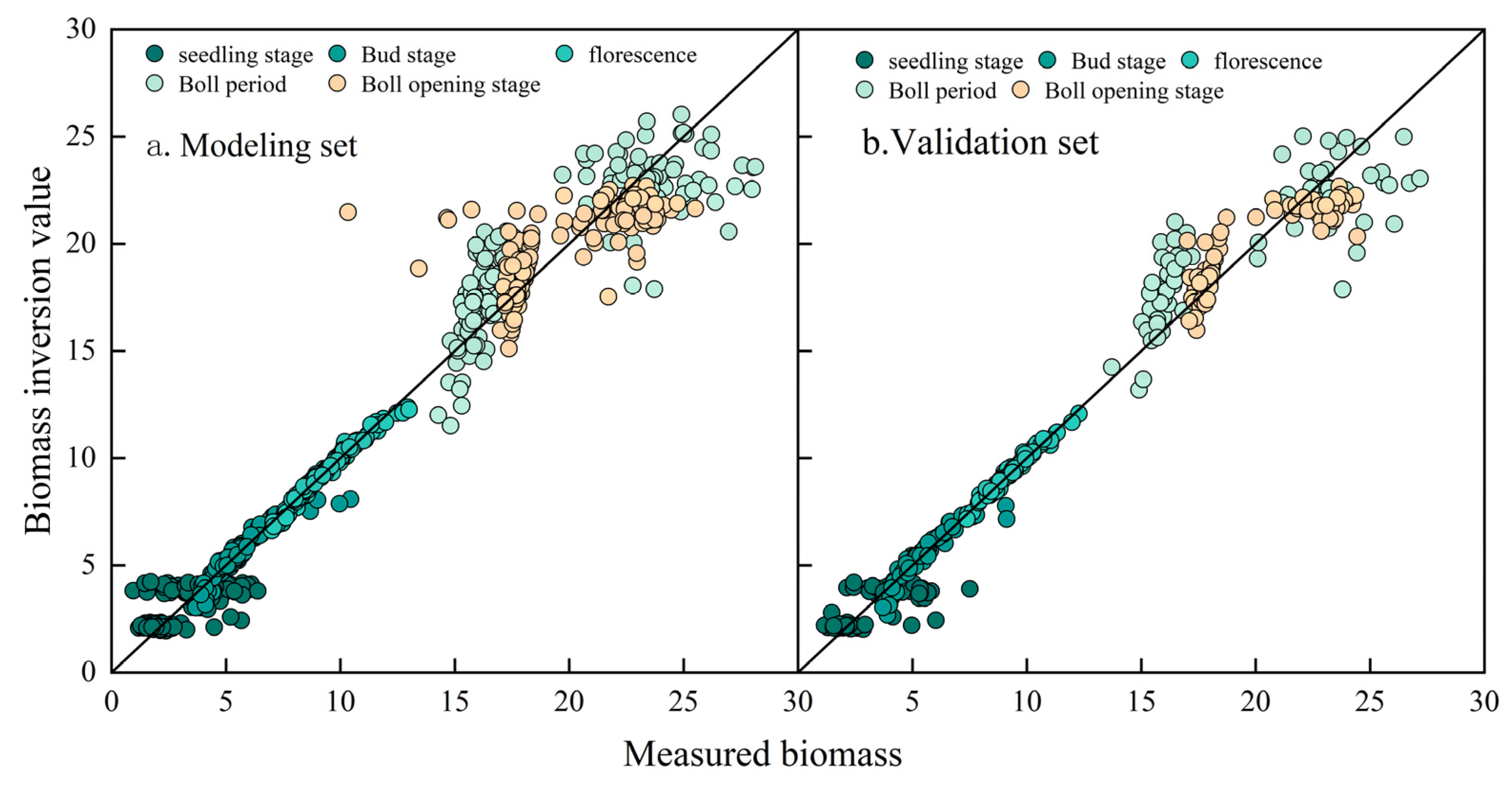
For AGB estimation, ridge regression models were developed based on the top five vegetation indices showing the highest gray relational degrees at key phenological stages of cotton. The experimental data from 2023 and 2024 were categorized into seedling (n = 216), budding (n = 216), flowering (n = 216), boll-setting (n = 216), and boll-opening (n = 216) stages. For each stage, 60% of the data were used for model training and 40% for validation. The performance metrics of the inversion models are presented in Figure 9 and Table 5.
The results show that the models constructed for the budding and flowering stages achieved the highest accuracy, suggesting that the VI-based inversion performs better during periods of rapid canopy expansion and biomass accumulation. The model for the boll-setting stage also exhibited good fitting accuracy, although with slightly higher RMSE, which may be attributed to increased structural complexity of the canopy and greater spectral interference during boll development. In contrast, the models for the seedling and boll-opening stages showed relatively lower accuracy, indicating that VIs are less sensitive to biomass variation during the early and late growth periods.
Overall, the ridge regression models effectively captured the spatiotemporal variation of AGB, particularly during the budding and flowering stages, demonstrating high prediction accuracy and generalization ability. Multi-stage modeling enhances adaptability across different phenological phases and reduces the instability associated with single-stage VI modeling.

3.3. AquaCrop Model Data Assimilation Based on Particle Swarm Optimization (PSO)

3.3.1. PSO Assimilation Process

To improve the accuracy of simulating cotton growth dynamics, this study developed an integrated AquaCrop-PSO model by optimizing key AquaCrop parameters using the Particle Swarm Optimization (PSO) algorithm and assimilating UAV remote sensing-derived aboveground biomass (AGB) and canopy cover (CC) as state variables. The integration process consisted of the following steps:
1. Sensitive Parameter Selection and Initialization
Based on the results of the EFAST sensitivity analysis, nine parameters with significant influence on CC and AGB simulations were selected (see Table 6 for detailed parameter descriptions). Initial positions and velocities of the particle swarm were assigned within the defined parameter bounds.
2. Model Execution and Output Simulation
The AquaCrop model executable “ACsaV70.exe” was run using PyChm-2rm Community Edition 2021.3.2 software, incorporating all necessary input data. The model simulated canopy cover (CCS) and aboveground biomass (AGBS).
3. Estimation of UAV Remote Sensing-Derived Values
Using the previously developed ridge regression inversion models, CC (CCr) and AGB (AGBr) were estimated based on UAV multispectral data collected in 2023 and 2024.
4. Cost Function Construction and PSO Iteration
A cost function was constructed using the differences between the model-simulated values (CCS and AGBS) and the UAV remote sensing estimates (CCr and AGBr). The PSO algorithm iteratively searched for the optimal parameter set that minimized the cost function. The selected cost function is defined as follows:
f = 1 n ( C C s C C r ) 2 + 1 n ( A G B s A G B r ) 2
This framework allowed the AquaCrop-PSO model to effectively integrate observational information into the simulation process, thereby enhancing model stability and prediction performance across different cotton growth stages.

3.3.2. Analysis of Optimal Fitness in PSO-Based Data Assimilation

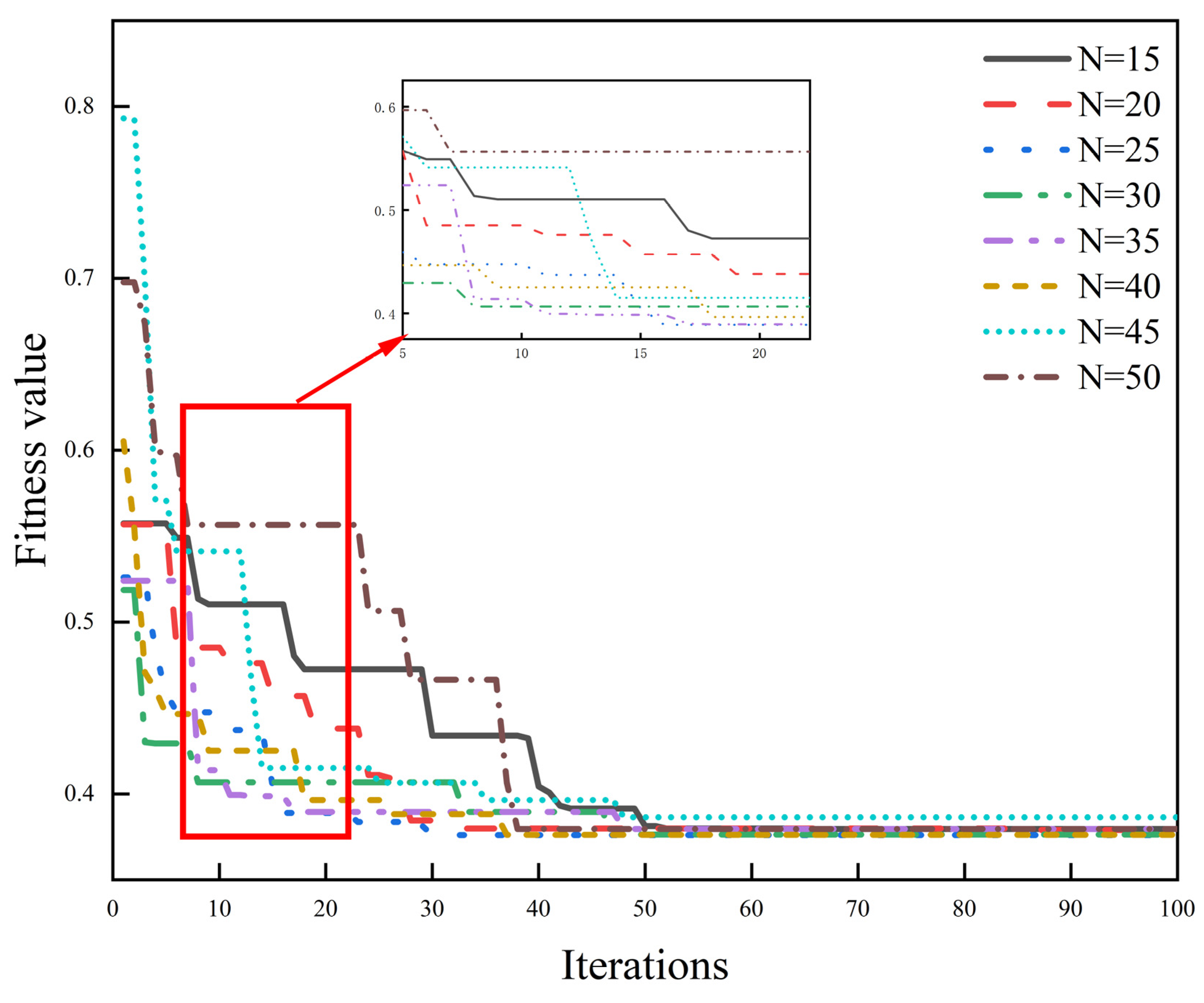
To determine the optimal particle swarm configuration, a series of PSO assimilation experiments was conducted using 2023 data, with the remotely sensed CCr and AGBr as assimilation targets. The number of particles was set to 15, 20, 25, 30, 35, 40, 45, and 50, respectively, and each configuration underwent 100 optimization iterations. The corresponding fitness values (lower values indicate better optimization results) and computation times were recorded.
As shown in Figure 10, the PSO algorithm demonstrated good convergence behavior during assimilation. The fitness value declined rapidly within the first 10 iterations, followed by a gradual decrease and stabilization. After approximately 35 iterations, the change in fitness values became marginal, indicating that the particle swarm was approaching the optimal solution.
Different particle numbers resulted in slight variations in convergence speed and final fitness values. Specifically, when the particle number was set to 30, the lowest final fitness value (About 0.379) was achieved with relatively short computation time. With 50 particles, the fitness value slightly decreased further to 0.376, but the runtime increased significantly (approximately 1017 s). In contrast, the setting with 45 particles yielded the highest initial fitness and converged to 0.393, indicating poorer performance.
Considering both optimization accuracy and computational efficiency, this study selected 35 particles and 40 iterations as the optimal configuration for the PSO algorithm. Under this configuration, the final fitness value stabilized at approximately 0.376, with an average computation time of around 262 s per plot, achieving a balance between efficiency and assimilation precision.

3.3.3. Estimation Results Based on the Assimilation Model

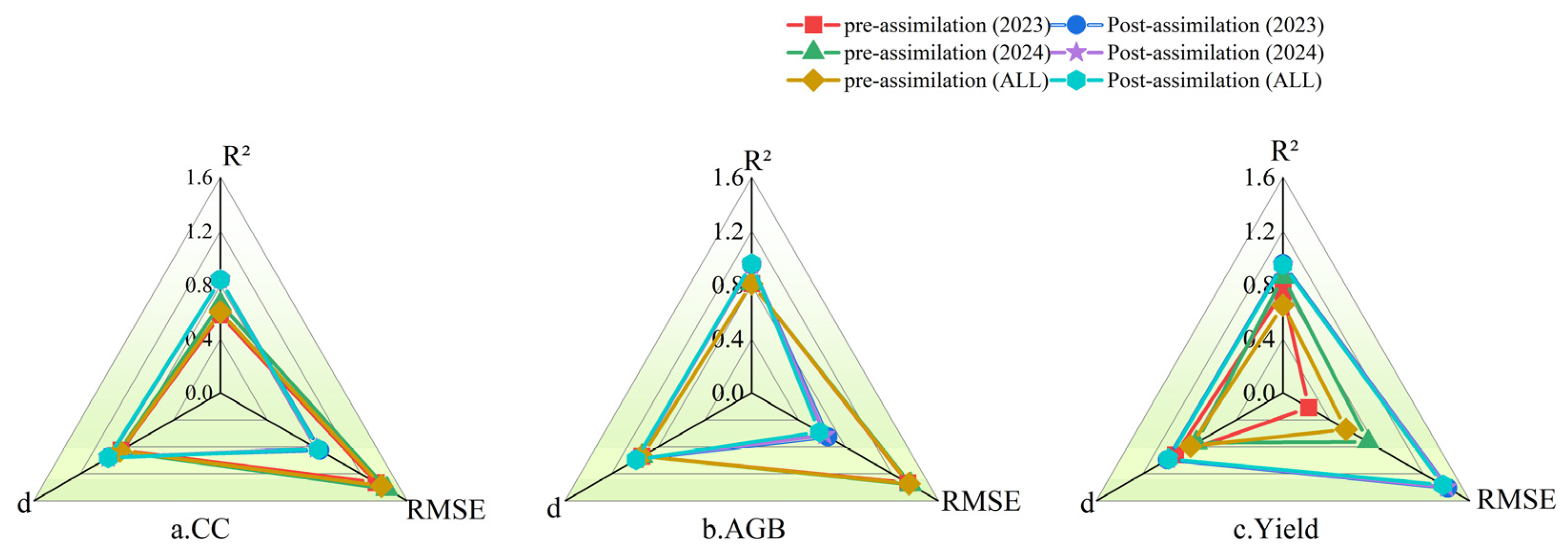
Figure 11 and Table 7 illustrate the simulation outcomes of the AquaCrop model following the assimilation of UAV remote sensing-derived canopy cover (CC) and aboveground biomass (AGB) as dual-state variables, together with a comparative analysis of model performance before and after assimilation. Overall, the AquaCrop-PSO assimilation framework substantially enhanced the simulation accuracy for AGB and yield (Y), and, to a certain extent, improved the model’s capability to reproduce CC dynamics.
The results indicated that, under the assimilation of CC and AGB as dual-state variables, the agreement between assimilated and observed CC was high, with R2 values of 0.84 and 0.84, RMSEs of 5.85% and 5.66%, and index of agreement (d) values of 0.95 and 0.96 for 2023 and 2024, respectively. In contrast, the assimilated and observed values of AGB and yield (Y) exhibited even higher consistency. For AGB, both 2023 and 2024 achieved identical R2 values of 0.95 and d values of 0.98, with RMSEs of 1.63 t·hm−2 and 1.57 t·hm−2, indicating stable assimilation performance across years. Yield estimation also demonstrated high accuracy, with R2 values of 0.96 in 2023 and 0.95 in 2024, RMSEs of 1.41 t·hm−2 and 1.40 t·hm−2, and d values of 0.99 and 0.98, reflecting consistently reliable yield simulations in both years.
The comparative analysis of pre- and post-assimilation results demonstrated that assimilating canopy cover (CC) and aboveground biomass (AGB) as dual-state variables into the AquaCrop model using PSO markedly enhanced its simulation performance. After assimilation, the coefficient of determination (R2) for CC increased from 0.58 and 0.66 in 2023 and 2024, respectively, to 0.84, while the root mean square error (RMSE) decreased from approximately 9.1% and 9.8% to 5.85% and 5.66%. The index of agreement (d) improved from 0.85–0.87 to 0.95–0.96. For AGB, R2 increased from 0.81 to 0.95, RMSE decreased from 3.34–3.40 t·hm−2 to 1.57–1.63 t·hm−2, and d increased from 0.94 to 0.98–0.99. Yield (Y) already exhibited high accuracy prior to assimilation (R2 = 0.75–0.86); however, post-assimilation R2 stabilized at 0.95–0.96, with RMSE reduced from 0.22–0.73 t·hm−2 to 1.37–1.41 t·hm−2, and d consistently maintained at 0.98–0.99. These results clearly indicate that dual-state variable assimilation is highly effective in reducing errors and improving both agreement and correlation.
In summary, assimilating CC and AGB as dual-state variables significantly enhanced the precision and stability of AquaCrop model simulations, particularly for AGB and yield estimation. These improvements provide an effective methodology for future irrigation management and yield forecasting in cotton production systems. However, certain uncertainties remain, such as potential errors from remote sensing inversion accuracy, parameter localization, and interannual climatic variability, which should be addressed in future applications to further improve model robustness.

3.4. Scenario Simulation Analysis Using the AquaCrop Model

3.4.1. Design of Irrigation Scenarios

To further investigate the impact of different irrigation regimes on cotton growth and water use efficiency, simulation experiments were conducted using the optimized AquaCrop-PSO model. Two types of irrigation scenarios were designed:
1. Variable Irrigation Quotas with Fixed Frequencies: Three irrigation quotas were set (330 mm, 420 mm, and 510 mm), each paired with four irrigation intervals (4, 5, 7, and 9 days), resulting in a total of 12 simulation scenarios. The irrigation amount per application was adjusted based on the total quota and frequency.
2. Fixed Irrigation Quotas with Variable Frequencies: Three fixed irrigation amounts per application were specified (33 mm, 42 mm, and 51 mm), combined with four irrigation intervals (4, 5, 7, and 9 days), also resulting in 12 scenarios, as shown in Table 8.
Historical meteorological data from 1963 to 2024 (a total of 61 years) for Daxi Canal Town, Changji City, were obtained from the China Meteorological Data Service Center. The annual precipitation sequence was fitted using the Pearson Type III distribution, and cumulative frequency analysis was applied to classify precipitation year types. According to the classification criteria, years with precipitation p ≤ 25% were defined as drought years, 25% < p < 75% as normal years, and p ≥ 75% as wet years. This classification approach effectively captures interannual variability in regional precipitation and supports the selection of representative climate years for scenario-based simulations. Based on this classification, the following years were selected for scenario simulation: wet years: 1987, 1988, 1998, 1999, 2007, 2016; normal years: 1966, 1971, 1972, 1980, 2010, 2011; dry years: 1963, 1978, 1983, 2009, 2012, 2021. Note that 2023 was classified as a normal year, while 2024 was categorized as a wet year.
For each of the two irrigation scenarios, twelve irrigation combinations were tested under each of the three precipitation categories. In total, 72 simulations (12 combinations × 3 precipitation types × 2 scenario types) were performed. Each scenario year included six representative years.
The model output was evaluated based on four criteria: cotton yield, aboveground biomass, water use efficiency (WUE), and total water consumption. These metrics were used to identify the optimal irrigation strategy for maximizing cotton production and resource efficiency under varying climatic conditions.

3.4.2. Simulation Results of Different Irrigation Scenarios

Based on the PSO-optimized AquaCrop model parameters, a total of 216 simulation scenarios were constructed, including three precipitation types (dry, normal, and wet years), six representative years for each type, two irrigation scenario types, and twelve irrigation treatments. The outputs included seed cotton yield (Y), aboveground biomass (AGB), water use efficiency (WUE), and evapotranspiration (ET). The ET values were dynamically simulated on a daily scale by the AquaCrop model, based on reference evapotranspiration (ET0) calculated using the FAO Penman–Monteith method, and adjusted through crop coefficient (Kc), soil evaporation coefficient (Ke), and water stress coefficient (Ks). Daily evaporation (E) and transpiration (Tr) were estimated accordingly and summed across the crop growth period to obtain the total ET. The simulation results for all scenarios are presented in Table 9 and Table 10.
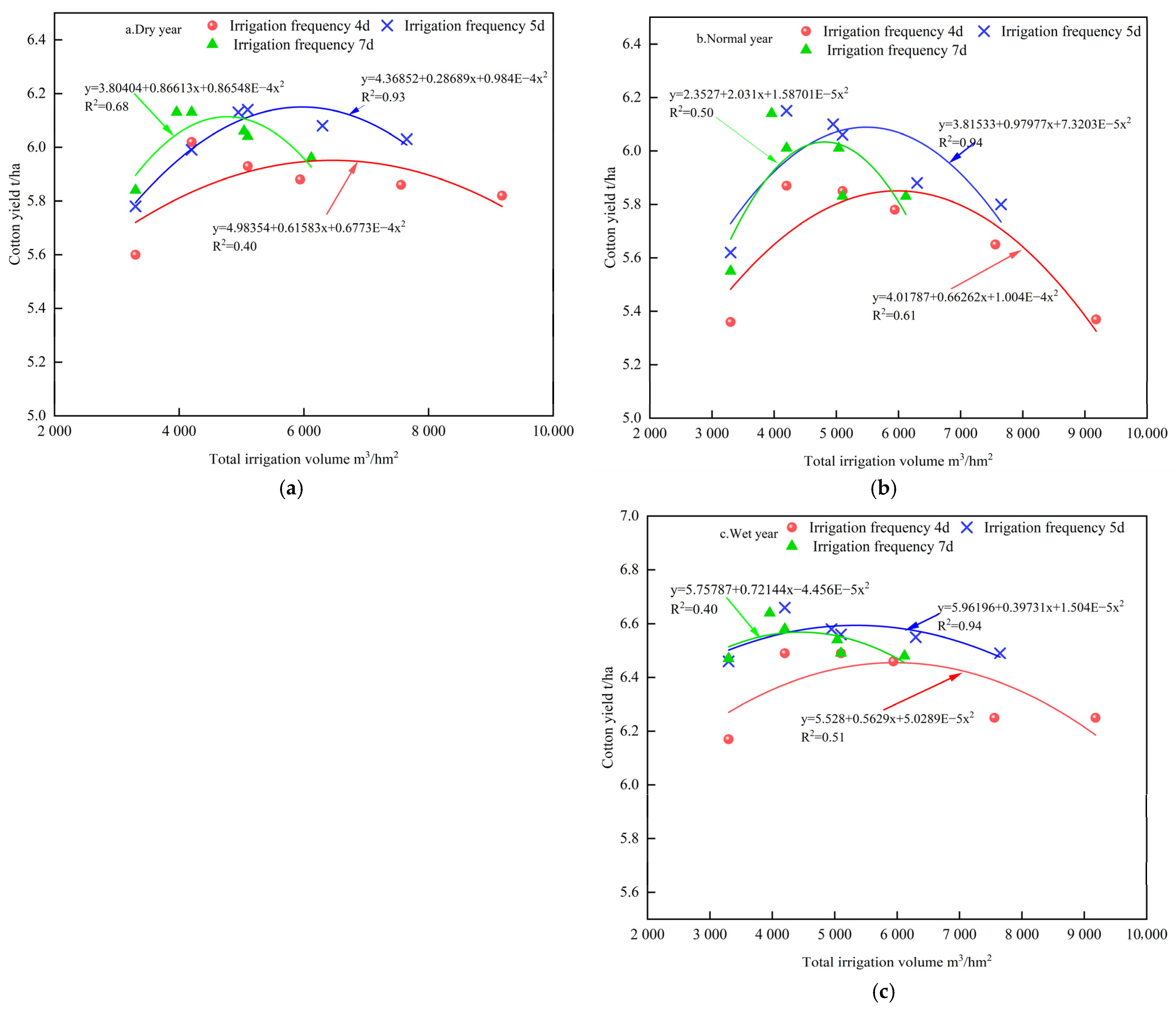
In Scenario Type I (fixed total irrigation quota with variable irrigation intervals), the average seed cotton yields across dry, normal, and wet years were 5.76 t·hm−2, 5.79 t·hm−2, and 6.42 t·hm−2, respectively. At a given total irrigation quota, both yield and biomass exhibited an initial increase followed by a decline as irrigation frequency increased. For example, in dry years, the highest yield (6.14 t·hm−2) was achieved under a quota of 510 mm with a 5-day irrigation interval. In normal and wet years, peak yields of 6.15 t·hm−2 and 6.56 t·hm−2 occurred under a 420 mm quota and 4-day interval. However, increasing irrigation frequency also led to reduced WUE and significantly increased ET, indicating that overly frequent irrigation, although meeting crop water requirements, may result in water wastage without proportional yield benefits.
In Scenario Type II (fixed irrigation amount per application with variable intervals), the average yields for dry, normal, and wet years were 5.79 t·hm−2, 5.86 t·hm−2, and 6.52 t·hm−2, respectively. Similar to Scenario I, yield initially increased and then declined with increasing irrigation frequency, with maximum yields generally occurring at a 5-day interval. Yields under 4-, 5-, and 7-day intervals consistently outperformed those under the 9-day interval. When the irrigation quota was fixed at 33 mm per application, WUE peaked at a 9-day interval across all precipitation types, reaching 0.83 kg·m−3 (dry year), 0.90 kg·m−3 (normal year), and 0.82 kg·m−3 (wet year), suggesting that under water-saving conditions, extending the irrigation interval can improve water use efficiency.
As shown in Figure 12, cotton yield exhibited a clear interactive response to total irrigation amount and frequency under different precipitation conditions. For instance, in dry years, when the total irrigation volume was below 5100 m3·hm−2, a 7-day interval yielded 6.13 t·hm−2; when irrigation volume exceeded 5100 m3·hm−2, the highest yield (6.14 t·hm−2) was achieved at a 5-day interval. In normal and wet years, yields were higher with a 7-day interval under irrigation volumes below 4200 m3·hm−2 (6.14 t·hm−2 and 6.64 t·hm−2, respectively), while a 5-day interval was more effective when volumes exceeded 4200 m3·hm−2 (6.15 t·hm−2 and 6.664 t·hm−2).
These findings underscore the importance of appropriately adjusting irrigation frequency and intensity to optimize cotton yield under varying precipitation regimes.
Considering both yield maximization and water conservation, the following optimal irrigation strategies are recommended based on simulation results:
Dry years: 5-day irrigation interval with a total irrigation volume of 5100 m3·hm−2 (Treatment P10);
Normal years: 5-day irrigation interval with a total irrigation volume of 4200 m3·hm−2 (Treatment P16);
Wet years: 5-day irrigation interval with a total irrigation volume of 4200 m3·hm−2 (Treatment P16).
These strategies achieve a balance between high and stable yields, water use efficiency, and water-saving irrigation, providing a practical technical reference for precision irrigation management in cotton production.

4. Discussion

This study utilized the EFAST sensitivity analysis method to identify the most influential parameters in the AquaCrop model for simulating cotton canopy cover (CC) and aboveground biomass (AGB). The results indicated that CGC, CCX, and CCS were the most critical for CC. Specifically, CGC (canopy growth coefficient) governs canopy expansion during early and mid-growth stages, making it particularly influential from the seedling to flowering stages. CCX defines the maximum canopy cover, while CCS represents the initial soil cover at emergence, both of which significantly affect simulation accuracy from emergence to full cover. These findings suggest that canopy cover dynamics are primarily constrained by early growth potential and mid-stage growth rates, with environmental factors such as temperature playing a lesser role in later stages.
For AGB, KCTRX, WP, and CGC were the most sensitive parameters. KCTRX reflects crop responsiveness to water stress during full canopy cover, WP (water productivity) represents the biomass produced per unit of transpiration, and CGC indirectly influences biomass accumulation rates. Given that AGB is a function of crop transpiration (Tr) and WP, the high sensitivity of KCTRX and WP indicates strong responsiveness of cotton growth to water dynamics, especially during mid to late developmental stages. These results are consistent with the physiological characteristics of cotton as a water-demanding crop.
Conducting sensitivity analysis of crop models allows for the effective identification of highly sensitive key parameters, thereby reducing the number of uncertain inputs, simplifying the model structure, and improving its applicability across diverse regions. For instance, Thorp et al. [37] employed the Sobol method to perform a global sensitivity analysis of the DSSAT-CROPGRO-Cotton model, successfully identifying approximately half of the parameters as having minimal influence on model outputs, thus streamlining the calibration process. Similarly, Pathak et al. [38] reported that global sensitivity analysis (GSA) provides more comprehensive insights into parameter contributions than local sensitivity methods, especially under both irrigated and rainfed cotton production systems. In addition, Mishra et al. [39] emphasized parameter sensitivity as a key focus in evaluating cotton yield simulations. Ghimire et al. [40] used multi-model simulations to explore how soil properties and management practices influence cotton yield and water productivity, further underscoring the importance of parameter selection. Although the studies by Martínez-Ruiz et al. [41] focused on tomato, respectively, both utilized EFAST or Sobol methods and demonstrated the broad applicability and robustness of global sensitivity analysis in crop modeling. Based on this, the EFAST method was employed in this study to conduct sensitivity analysis on 26 parameters, providing a theoretical basis for parameter localization and subsequent remote sensing data assimilation.
Regarding vegetation index inversion, the study found that indices such as GNDVI, TVI, NDVI, NBI, and NDRE were highly correlated with CC, with GNDVI showing the highest R2 value (0.85). The ridge regression model integrating multiple vegetation indices outperformed single-index models, demonstrating its capacity to comprehensively capture canopy dynamics. Vegetation indices, derived from crop reflectance in visible and near-infrared bands, effectively reflect changes in canopy structure and biomass [42]. Numerous studies [43,44,45,46] have similarly used VIs for LAI or biomass inversion with high accuracy. In this study, the inversion models for AGB during the squaring and flowering stages achieved R2 values of 0.97 and 0.87, respectively, significantly outperforming those for the seedling and boll-opening stages (0.41 and 0.46). This indicates that the mid-growth stages are critical for biomass accumulation and most sensitive to remote sensing monitoring.
In terms of model assimilation, the AquaCrop-PSO model efficiently integrated UAV remote sensing data with crop simulations. Using AGB and CC as dual-state variables, the model substantially improved yield prediction accuracy, with R2 values of 0.96 and 0.95 in 2023 and 2024, respectively. As AGB directly contributes to yield and CC reflects the photosynthetically active structure, their combined assimilation enhances both the spatial and temporal simulation accuracy and model stability. Prior studies [47,48,49] also confirmed the effectiveness of remote sensing data assimilation in improving model performance.
Simulation results under three typical precipitation scenarios—dry, normal, and wet years—indicated that moderately increasing irrigation frequency can improve both water use efficiency (WUE) and yield. However, excessively high frequencies may lead to yield reductions due to root zone hypoxia or water wastage. For instance, in dry years, the highest yield (6.14 t·hm−2) was achieved under a total irrigation amount of 5100 m3·hm−2 with a 5-day interval. Similarly, in normal and wet years, the optimal performance was observed with a total irrigation of 4200 m3·hm−2 at the same frequency. These results suggest that a moderate irrigation amount combined with an appropriate frequency is most favorable for balancing water use and yield in cotton fields. From the perspective of WUE and evapotranspiration (ET) regulation, irrigation frequency had a greater influence on model outputs than irrigation quota, indicating that future water-saving irrigation strategies should prioritize frequency regulation. It is worth noting that previous studies have also supported the conclusions of this research. For example, Autovino et al. [50] integrated crop water production functions, irrigation uniformity, and economic evaluations to develop a more scientific and efficient irrigation decision-making framework. Their findings emphasized that optimizing irrigation frequency and water allocation can significantly enhance both water use efficiency and economic returns without substantially compromising yield. This provides further theoretical and practical support for the effectiveness of the “moderate amount + appropriate frequency” strategy proposed in this study. Although the AquaCrop model has been widely applied to optimize irrigation strategies for various crops such as wheat [51], maize [52], rice [53], soybean [54], and sugarcane [55], parameter calibration still largely relies on expert knowledge and manual adjustment, which limits modeling efficiency and adaptability. To address this issue, this study incorporated the Particle Swarm Optimization (PSO) algorithm to systematically calibrate model parameters and achieve automated simulation of cotton field irrigation scheduling under typical climatic conditions.
By integrating UAV remote sensing, EFAST parameter sensitivity analysis, and PSO optimization, this study achieved parameter localization, constructed accurate inversion models, and effectively assimilated UAV remote sensing data into the AquaCrop model. The resulting AquaCrop-PSO model provides a robust tool for simulating optimized irrigation strategies under different climate scenarios. However, this study was conducted under the specific climatic conditions of Changji, Xinjiang, and thus further validation and optimization are needed for broader applicability. Future work should explore the model’s performance in other arid regions and expand its use to additional crop types to improve its generalizability and support sustainable modern agricultural practices.

5. Conclusions

This study integrated field experiments with UAV remote sensing inversion, machine learning algorithms, and crop model simulations to investigate the effects of drip irrigation intervals and frequencies on cotton growth dynamics and yield. It also proposed an optimized irrigation scheduling strategy. The main conclusions are as follows:
(1) Sensitivity analysis of the AquaCrop model indicated that the canopy growth coefficient (CGC), maximum canopy cover (CCX), and canopy cover at 90% emergence (CCS) were the key parameters influencing canopy cover (CC). For aboveground biomass (AGB), the most sensitive parameters were the crop coefficient at full canopy but before senescence (KCTRX), water productivity (WP), and CGC. By selecting and localizing these key parameters, the accuracy and efficiency of model simulations and data assimilation were effectively improved. This also provided a solid foundation for parameter optimization in the AquaCrop-PSO assimilation process, enabling more accurate simulations of CC and AGB and enhancing the model’s applicability for evaluating and optimizing irrigation regimes.
(2) The ridge regression model based on multiple vegetation indices demonstrated superior performance in estimating CC and AGB compared to single-index linear regression models. The integration of multiple vegetation indices significantly enhanced the inversion accuracy, confirming the model’s high adaptability to crop phenological changes and its ability to support stage-specific predictions.
(3) Assimilation of both CC and AGB as dual-state variables substantially improved the model’s predictive accuracy. The R2 values for CC assimilation were 0.84 and 0.84 in 2023 and 2024, respectively; for AGB, the R2 was consistently 0.95. The yield simulation achieved R2 values of 0.96 and 0.95 in the respective years. These results demonstrate the robustness and cross-year generalization capability of the AquaCrop-PSO assimilation framework in representing cotton growth processes and yield variation.
(4) Scenario simulations using the AquaCrop-PSO model under two representative irrigation conditions indicated that, in dry years, the optimal irrigation strategy involves a 5-day irrigation interval with a total irrigation quota of 5100 m3·hm−2. In normal and wet years, the recommended irrigation frequency remains 5 days, with a total irrigation quota of 4200 m3·hm−2. These optimized results provide quantitative support and practical guidance for the design of precision water-saving irrigation strategies in arid cotton-growing regions.
While the present study demonstrated the effectiveness of integrating UAV-based remote sensing, PSO optimization, and the AquaCrop model for irrigation scheduling, several research gaps remain to be addressed. For instance, the current framework primarily focuses on a single crop and regional context, which may limit its transferability to other cropping systems or agro-ecological zones. Future research could explore the operational scalability of the approach in diverse field conditions and at larger spatial scales. Moreover, enhancing sensor fusion—such as combining UAV data with ground-based soil moisture, weather, and plant physiological sensors—could improve the temporal resolution and robustness of model inputs. Additionally, the integration of artificial intelligence (AI) techniques, such as deep learning or hybrid ensemble models, may facilitate more automated, adaptive, and accurate irrigation decision-making. Addressing these gaps would contribute to building a more generalizable, intelligent, and data-driven irrigation management framework for sustainable agriculture under climate uncertainty.

Author Contributions

Q.F. and M.H. designed the experiment. F.W. and D.Z. conducted the experiment. F.W. wrote the manuscript. Q.F., W.T., L.S., and Q.W. critically reviewed and edited the manuscript. All authors have read and agreed to the published version of the manuscript.

Funding

This study was funded by the Major Science and Technology Project of the Xinjiang Uygur Autonomous Region (No. 2022A02011-2), the Earmarked Fund for the China Agriculture Research System (CARS-15-13), and the Major Science and Technology Project of the Xinjiang Uygur Autonomous Region (No. 2023A02002-5).

Data Availability Statement

The data presented in this study are available in the figures and tables provided in the manuscript.

Acknowledgments

We appreciate and thank the anonymous reviewers for helpful comments that led to an overall improvement of the manuscript. We also thank the Journal Editor Board for their help and patience throughout the review process.

Conflicts of Interest

The authors declare no conflicts of interest.

Appendix A

Table A1. Calculation formula of vegetation index.
Vegetation Index Calculation FormulaReferences
NDVI N D V I = N I R R e d N I R + R e d [56]
SR S R = N I R R e d [57]
SAVI S A V I = 1.5 × N I R R e d N I R + R e d + 0.5 [58]
EVI E V I = 2.5 × N I R R e d N I R + 6 R e d 7.5 B l u e + 1 [58]
GNDVI G N D V I = N I R G r e e n N I R + G r e e n [58]
NGRDI N G R D I = G r e e n R e d G r e e n + R e d [59]
NPCI N P C I = R e d B l u e R e d + B l u e [60]
TVI T V I = N D V I + 0.5 [33]
VARI V A R I = G r e e n R e d G r e e n + R e d b l u e [61]
MSAVI M S A V I = 2 N I R + 1 ( 2 N I R + 1 ) 2 8 ( N I R R e d ) 2 [58]
OSAVI O S A V I = N I R R e d N I R + R e d + 0.16 [58]
WDVI W D V I = N I R 0.5 × R e d [62]
PSRI P S R I = R e d G r e e n N I R [63]
TCARI T C A R I = 3 × ( R e d e d g e R e d 0.2 × ( R e d e d g e + G r e e n ) × R e d e d g e R e d ) [64]
MCARI M C A R I = 1.2 × ( 2.5 × N I R R e d 1.3 × N I R G r e e n ) [37]
DVI D V I = N I R R e d [62]
IPVI I P V I = N I R N I R + R e d [65]
MTVI M T V I = 1.2 × ( 1.2 × N I R G r e e n 2.5 × R e d G r e e n ) [64]
NBI N B I = R e d e d g e N I R R e d e d g e + N I R [66]
GCVI G C V I = N I R G r e e n 1 [67]
NDRE N D R E = N I R R e d e d g e N I R + R e d e d g e [68]
MSR M S R = N I R R e d 1 N I R R e d + 1 [69]
Table A2. Variation range of crop parameters of AquaCrop model.
ParametersDescribeParameter Variation Range (±35%)
TBASEBase temperature7.8–16.2
TUPPERUpper temperature22.75–47.25
PEXPUPPERSoil water depletion factor for canopy expansion (p-exp)—upper threshold0.13–0.27
PEXPLOWERSoil water depletion factor for canopy expansion (p-exp)—lower threshold0.455–0.945
SFEShape factor for water stress coefficient for canopy expansion (0.0 = linear)1.625–3.375
SFCShape factor for stomatal control coefficient (0.0 = linear)1.95–4.05
PSENSoil water depletion factor for canopy senescence (p-sen)—upper threshold0.4875–1.0125
SFSShape factor for canopy senescence stress coefficient (0.0 = linear)1.625–3.375
PPOLSoil water depletion factor for pollination (p-pol)—upper threshold0.5525–1.1475
KCTRXCrop coefficient when canopy is complete but prior to senescence (KcTr,x)0.715–1485
KCDCLDecline rate of crop coefficient (%/day) due to senescence, nitrogen deficiency, etc.0.195–0.405
ZNMinimum effective rooting depth (m)0.195–0.405
ZXMaximum effective rooting depth (m)1.3–2.7
RTSHPShape factor describing root zone expansion9.75–20.25
RTEXUPMaximum root water extraction in the top quarter of the root zone (m3 water/m3 soil·day)0.0312–0.0648
RTEXLWMaximum root water extraction in the bottom quarter of the root zone (m3 water/m3 soil·day)0.0078–0.0162
EVLADCEffect of late-stage canopy cover on reducing soil evaporation39–81
CCSSoil area covered by a single seedling at 90% emergence (cm2)3.9–8.1
CSOCanopy size of a single plant on the first day after regeneration (cm2)3.9–8.1
DENNumber of plants per hectare78,000–162,000
CGCCanopy growth coefficient (CGC): Rate of increase in canopy cover0.049472–0.102749
CCXMaximum canopy cover (CCx): Fraction of soil covered0.637–1.323
SDCCanopy decline coefficient (CDC): Rate of canopy cover decrease (fraction/day)0.018961–0.03938
WPWater Productivity (WP): Normalized biomass per transpired water with reference CO2 (g/m2)9.75–20.25
HIReference harvest index (HIo) (%)32.5–67.5
SHIMaximum allowable increase in harvest index (%)19.5–40.5

References

  1. Guan, Y.; Tian, X.; Zhang, W.; Marino, A.; Huang, J.; Mao, Y.; Zhao, H. Forest canopy cover inversion exploration using multi-source optical data and combined methods. Forests 2023, 14, 1527. [Google Scholar] [CrossRef]
  2. Li, L.; Shikun, S.; Jing, X.; Zihan, G.; Jinfeng, Z.; Yali, Y.; Fei, G.; Xiaobo, L. Crop yield estimation based on assimilation of crop models and remote sensing data: A systematic evaluation. Agric. Syst. 2023, 210, 103711. [Google Scholar] [CrossRef]
  3. Huang, J.; Ma, H.; Sedano, F.; Lewis, P.; Liang, S.; Wu, Q.; Su, W.; Zhang, X.; Zhu, D. Evaluation of regional estimates of Winter wheat yield by assimilating three remotely sensed reflectance datasets into the coupled WOFOST–PROSAIL model. Eur. J. Agron. 2019, 102, 1–13. [Google Scholar] [CrossRef]
  4. Weiss, M.; Baret, F.; Myneni, R.B.; Pragnère, A.; Knyazikhin, Y. Investigation of a model inversion technique to estimate canopy biophysical variables from spectral and directional reflectance data. Agronomie 2000, 20, 3–22. [Google Scholar] [CrossRef]
  5. Verrelst, J.; Rivera, J.P.; Veroustraete, F.; Muñoz-Marí, J.; Clevers, J.G.P.W.; Camps-Valls, G.; Moreno, J. Experimental sentinel-2 lai estimation using parametric, non-parametric and physical retrieval methods—A comparison. ISPRS J. Photogramm. Remote Sens. 2015, 108, 260–272. [Google Scholar] [CrossRef]
  6. Thorp, K.R.; Hunsaker, D.J.; French, A.N. Assimilating leaf area index estimates from remote sensing into the simulations of a cropping systems model. Trans. ASABE 2010, 53, 251–262. [Google Scholar] [CrossRef]
  7. Richter, R.; Schlapfer, D. Geo-atmospheric processing of airborne imaging spectrometry data. Part 2: Atmospheric/topographic correction. Int. J. Remote Sens. 2002, 23, 2631–2649. [Google Scholar] [CrossRef]
  8. Marissa, K.; Noemi, V.; Hamze, D. A comprehensive assessment of in situ and remote sensing soil moisture data assimilation in the APSIM model for improving agricultural forecasting across the US Midwest. Hydrol. Earth Syst. Sci. 2023, 27, 1173–1199. [Google Scholar] [CrossRef]
  9. Wang, P.; Sun, H.; Xie, Y.; Wang, L.; Zang, S.; Li, L. Winter wheat yield estimation based on four-dimensional variational assimilation and ensemble Kalman filter methods. Trans. Chin. Soc. Agric. Eng. 2015, 31, 187–195. [Google Scholar]
  10. Akhavizadegan, F.; Ansarifar, J.; Wang, L.; Huber, I.; Archontoulis, S.V. A time-dependent parameter estimation framework for crop modeling. Sci. Rep. 2021, 11, 11437. [Google Scholar] [CrossRef]
  11. Jiang, K.A.; Zhao, J.; Luo, Y.; Cao, J.; Ying, L. Spectral characteristics analysis and inversion of rice leaf chlorophyll using RNCA-PSO-ELM. Trans. Chin. Soc. Agric. Eng. 2022, 38, 178–186. [Google Scholar]
  12. Liu, F.L.; Dong, C.; Wang, Y.; Wang, Q.; Huang, J.; Jiang, W. Crop growth monitoring based on data assimilation between remote sensing data and crop growth models. Trans. Chin. Soc. Agric. Eng. 2011, 27, 101–106. [Google Scholar]
  13. Marta, A.D.; Chirico, G.B.; Bolognesi, S.F.; Mancini, M.; D’Urso, G.; Orlandini, S.; Michele, C.D.; Altobelli, F. Integrating sentinel-2 imagery with AquaCrop for dynamic assessment of tomato water requirements in southern Italy. Agronomy 2019, 9, 404. [Google Scholar] [CrossRef]
  14. Upreti, D.; Pignatti, S.; Pascucci, S.; Tolomio, M.; Huang, W.; Casa, R. Bayesian calibration of the AquaArop-OS model for Durum wheat by assimilation of canopy cover retrieved from VENμS satellite data. Remote Sens. 2020, 12, 2666. [Google Scholar] [CrossRef]
  15. Yokoyama, Y.; Wit, A.d.; Matsui, T.; Tanaka, T.S.T. Accuracy and robustness of a plant-level Cabbage yield prediction system generated by assimilating UAV-based remote sensing data into a crop simulation model. Precis. Agric. 2024, 25, 2685–2702. [Google Scholar] [CrossRef]
  16. Wagner, M.P.; Slawig, T.; Taravat, A.; Oppelt, N. Remote sensing data assimilation in dynamic crop models using particle swarm optimization. ISPRS Int. J. Geo Inf. 2020, 9, 105. [Google Scholar] [CrossRef]
  17. Dlamini, L.; Crespo, O.; Dam, J.V.; Kooistra, L. A global systematic review of improving crop model estimations by assimilating remote sensing data: Implications for small-scale agricultural systems. Remote Sens. 2023, 15, 4066. [Google Scholar] [CrossRef]
  18. Zare, H.; Weber, T.K.; Ingwersen, J.; Nowak, W.; Gayler, S.; Streck, T. Within-season crop yield prediction by a multi-model ensemble with integrated data assimilation. Field Crops Res. 2024, 308, 109293. [Google Scholar] [CrossRef]
  19. Novelli, F.; Vuolo, F. Assimilation of sentinel-2 leaf area index data into a physically-based crop growth model for yield estimation. Agronomy 2019, 9, 255. [Google Scholar] [CrossRef]
  20. Liu, J.; Hou, X.; Chen, S.; Mu, Y.; Huang, H.; Wang, H.; Liu, Z.; Li, S.; Zhang, X.; Zhao, Y.; et al. A method for estimating yield of maize inbred lines by assimilating WOFOST model with sentinel-2 satellite data. Front. Plant Sci. 2023, 14, 1201179. [Google Scholar] [CrossRef]
  21. Pazhanivelan, S.; Geethalakshmi, V.; Tamilmounika, R.; Sudarmanian, N.S.; Kaliaperumal, R.; Ramalingam, K.; Sivamurugan, A.P.; Mrunalini, K.; Yadav, M.K.; Quicho, E.D. Spatial rice yield estimation using multiple linear regression analysis, semi-physical approach and assimilating SAR satellite derived products with DSSAT crop simulation model. Agronomy 2022, 12, 2008. [Google Scholar] [CrossRef]
  22. Gaso, D.V.; Paudel, D.; de Wit, A.; Puntel, L.A.; Mullissa, A.; Kooistra, L. Beyond assimilation of leaf area index: Leveraging additional spectral information using machine learning for site-specific soybean yield prediction. Agric. For. Meteorol. 2024, 351, 110022. [Google Scholar] [CrossRef]
  23. Ines, A.V.M.; Das, N.N.; Hansen, J.W.; Njoku, E.G. Assimilation of remotely sensed soil moisture and vegetation with a crop simulation model for maize yield prediction. Remote Sens. Environ. 2013, 138, 149–164. [Google Scholar] [CrossRef]
  24. Chunyan, M.; Mingxing, L.; Fan, D.; Changchun, L.; Yingqi, C.; Weinan, C.; Yilin, W. Wheat growth monitoring and yield estimation based on remote sensing data assimilation into the SAFY crop growth model. Sci. Rep. 2022, 12, 5473. [Google Scholar] [CrossRef]
  25. Curnel, Y.; Wit, A.J.W.D.; Duveiller, G.; Defourny, P. Potential performances of remotely sensed lai assimilation in WOFOST model based on an OSS experiment. Agric. For. Meteorol. 2011, 151, 1843–1855. [Google Scholar] [CrossRef]
  26. Daniels, L.; Eeckhout, E.; Wieme, J.; Dejaegher, Y.; Audenaert, K.; Maes, W.H. Identifying the optimal radiometric calibration method for UAV-based multispectral imaging. Remote Sens. 2023, 15, 2909. [Google Scholar] [CrossRef]
  27. Tao, H.B.; Lin, B. Comparison on disc method with copy method and length-width method for measuring leaf area of rice. Plant Physiol. Commun. 2006, 42, 496–498. [Google Scholar]
  28. Wang, F. Study on Remote Sensing Yield Estimation Methods for Rice Based on Multi-Source Data from Satellite and UAV. Master’s Thesis, Zhejiang University, Hangzhou, China, 2019. [Google Scholar]
  29. Motohka, T.; Nasahara, K.N.; Oguma, H.; Tsuchida, S. Applicability of green-red vegetation index for remote sensing of vegetation phenology. Remote Sens. 2010, 2, 2369. [Google Scholar] [CrossRef]
  30. Shu, Z.; Jin, J.; Menzel, L.; Zhang, J.; Luo, J.; Wang, G.; Cui, N.; Guan, T.; Liu, Y. Evaluating the effectiveness of different surface resistance schemes coupled with penman-monteith model for estimating actual evapotranspiration—A global comparative study. J. Hydrol. 2025, 656, 133047. [Google Scholar] [CrossRef]
  31. Steduto, P.; Hsiao, T.C.; Raes, D.; Fereres, E. Aquacrop—The FAO crop model to simulate yield response to water: I. Concepts and underlying principles. Agron. J. 2009, 101, 426–437. [Google Scholar] [CrossRef]
  32. Jin, X.-L.; Feng, H.-K.; Zhu, X.-K.; Li, Z.-H.; Song, S.-N.; Song, X.-Y.; Yang, G.-J.; Xu, X.-G.; Guo, W.-S. Assessment of the AquaCrop model for use in simulation of irrigated Winter wheat canopy cover, biomass, and grain yield in the north China plain. PLoS ONE 2017, 9, e86938. [Google Scholar] [CrossRef]
  33. Broge, N.H.; Leblanc, E. Comparing prediction power and stability of broadband and hyperspectral vegetation indices for estimation of green leaf area index and canopy chlorophyll density. Remote Sens. Environ. 2001, 76, 156–172. [Google Scholar] [CrossRef]
  34. Xing, H.X.; Xu, S.; Chen, X.; Feng, Y.; Yang, H.; Chen, G.; Zhao, X. Global sensitivity analysis of AquaCrop crop model parameters using the E-FAST method. Sci. Agric. Sin. 2017, 50, 64–76. [Google Scholar]
  35. Gordillo-Salinas, V.M.; Flores-Magdaleno, H.; Ortiz-Solorio, C.A.; Arteaga-Ramírez, R. Evaluation of nitrogen status in a wheat crop using unmanned aerial vehicle images. Chil. J. Agric. Res. 2021, 81, 408–419. [Google Scholar] [CrossRef]
  36. Lacerda, L.N.; Snider, J.; Cohen, Y.; Liakos, V.; Levi, M.R.; Vellidis, G. Correlation of UAV and satellite-derived vegetation indices with cotton physiological parameters and their use as a tool for scheduling variable rate irrigation in cotton. Precis. Agric. 2022, 23, 2089–2114. [Google Scholar] [CrossRef]
  37. Thorp, K.; Marek, G.; DeJonge, K.; Evett, S. Comparison of evapotranspiration methods in the DSSAT cropping system model: I. Global sensitivity analysis. Comput. Electron. Agric. 2020, 177, 105679. [Google Scholar] [CrossRef]
  38. Pathak, T.B.; Fraisse, C.W.; Jones, J.W.; Messina, C.D.; Hoogenboom, G. Use of global sensitivity analysis for CROPGRO cotton model development. Trans. ASABE 2007, 50, 2295–2302. [Google Scholar] [CrossRef]
  39. Kumar, M.S.; Varinderjit, K.; Kulvir, S. Evaluation of DSSAT-CROPGRO-cotton model to simulate phenology, growth, and seed cotton yield in northwestern India. Agron. J. 2021, 113, 3975–3990. [Google Scholar] [CrossRef]
  40. Ghimire, B.; Adedeji, O.; Ritchie, G.L.; Guo, W. Simulating crop yields and water productivity for three cotton-based cropping systems in the Texas high plains. Crop Environ. 2025, 4, 83–96. [Google Scholar] [CrossRef]
  41. Martínez-Ruiz, A.; Ruiz-García, A.; Prado-Hernández, J.V.; López-Cruz, I.L.; Valencia-Islas, J.O.; Pineda-Pineda, J. Global sensitivity analysis and calibration by differential evolution algorithm of HortSyst crop model for fertigation management. Water 2021, 13, 610. [Google Scholar] [CrossRef]
  42. Nandan, R.; Bandaru, V.; He, J.; Daughtry, C.; Gowda, P.; Suyker, A.E. Evaluating optical remote sensing methods for estimating leaf area index for Corn and Soybean. Remote Sens. 2022, 14, 5301. [Google Scholar] [CrossRef]
  43. Jiang, Y.; Zhang, Z.; He, H.; Zhang, X.; Feng, F.; Xu, C.; Zhang, M.; Lafortezza, R. Research on leaf area index inversion based on less 3d radiative transfer model and machine learning algorithms. Remote Sens. 2024, 16, 3627. [Google Scholar] [CrossRef]
  44. Yan, G.; Kaili, Y.; Zhiheng, L.; Shenghui, F.; Xianting, W.; Renshan, Z.; Yi, P. Remote estimation of leaf area index (lai) with unmanned aerial vehicle (UAV) imaging for different rice cultivars throughout the entire growing season. Plant Methods 2021, 17, 88. [Google Scholar] [CrossRef] [PubMed]
  45. Mukiibi, A.; Machakaire, A.T.B.; Franke, A.C.; Steyn, J.M. A systematic review of vegetation indices for Potato growth monitoring and tuber yield prediction from remote sensing. Potato Res. 2024, 68, 409–448. [Google Scholar] [CrossRef]
  46. Li, C.; Cui, Y.; Ma, C.; Niu, Q.; Li, J. Hyperspectral inversion of maize biomass coupled with plant height data. Crop Sci. 2021, 61, 2067–2079. [Google Scholar] [CrossRef]
  47. Gumma, M.K.; Kadiyala, M.D.M.; Panjala, P.; Ray, S.S.; Akuraju, V.R.; Dubey, S.; Smith, A.P.; Das, R.; Whitbread, A.M. Assimilation of remote sensing data into crop growth model for yield estimation: A case study from India. J. Indian. Soc. Remote Sens. 2021, 50, 257–270. [Google Scholar] [CrossRef]
  48. De Wit, A.J.W.; van Diepen, C.A. Crop model data assimilation with the ensemble Kalman filter for improving regional crop yield forecasts. Agric. For. Meteorol. 2007, 146, 38–56. [Google Scholar] [CrossRef]
  49. Xing, H.L.; Xu, Z.; Feng, X.; Yang, H.; Chen, G.; Xia, Z. Comparison of multiple data assimilation algorithms based on remote sensing and the AquaCrop crop model. Trans. Chin. Soc. Agric. Eng. 2017, 33, 183–192. [Google Scholar]
  50. Autovino, D.; Provenzano, G.; Monserrat, J.; Cots, L.; Barragán, J. Determining optimal seasonal irrigation depth based on field irrigation uniformity and economic evaluations: Application for onion crop. J. Irrig. Drain. Eng. 2016, 142, 04016037. [Google Scholar] [CrossRef]
  51. Tafteh, A.; Emdad, M.R.; Sedaghat, A. Improving irrigation management in wheat farms through the combined use of the AquaCrop and WinSRFR models. J. Arid. Land. 2025, 17, 245–258. [Google Scholar] [CrossRef]
  52. Sharafkhane, M.G.; Ziaei, A.N.; Naghedifar, S.M.; Akbari, A.; Verdi, A. AquaCrop Plug-in-PSO: A novel irrigation scheduling optimization framework for maize to maximize crop water productivity using in-season weather forecast and crop yield estimation. Agric. Water Manag. 2024, 306, 109153. [Google Scholar] [CrossRef]
  53. Sayadi, F.J.; Sefidkouhi, M.A.G.; Pirdashti, H.; Khoshravesh, M. Assimilating vegetation indices and canopy cover derived from remote sensing into the AquaCrop model for estimating rice yield. Irrig. Drain. 2024, 74, 1311–1325. [Google Scholar] [CrossRef]
  54. Giménez, L.; Paredes, P.; Pereira, L.S.; Xu, Y.J. Water use and yield of soybean under various irrigation regimes and severe water stress. Application of AquaCrop and SIMDualkc models. Water 2017, 9, 393. [Google Scholar] [CrossRef]
  55. Mostafa, R.J.; Farhad, M.; Abdolmajid, L. Evaluation of Sugarcane irrigation using AquaCrop model and remote sensing. Irrig. Drain. 2022, 71, 1034–1047. [Google Scholar] [CrossRef]
  56. Farias, G.D.; Bremm, C.; Bredemeier, C.; Menezes, J.D.L.; Alves, L.A.; Tiecher, T.; Martins, A.P.; Fioravanço, G.P.; da Silva, G.P.; Carvalho, P.C.D.F. Normalized Difference Vegetation Index (NDVI) for Soybean biomass and nutrient uptake estimation in response to production systems and fertilization strategies. Front. Sustain. Food Syst. 2023, 6, 959681. [Google Scholar] [CrossRef]
  57. Liang, B.L.; Hao, X.; Chu, Y.; Tang, B.; Sheng, Z. Estimation of vegetation biomass in arid desert regions based on five vegetation indices. Arid. Zone Res. 2023, 40, 647–654. [Google Scholar] [CrossRef]
  58. Dorijan, R.; Ante, Š.; Rajko, M.; Mladen, J. State of major vegetation indices in precision agriculture studies indexed in web of science: A review. Agriculture 2023, 13, 707. [Google Scholar] [CrossRef]
  59. Hunt, E.R.; Cavigelli, M.; Daughtry, C.S.T.; Mcmurtrey, J.E.; Walthall, C.L. Evaluation of digital photography from model aircraft for remote sensing of crop biomass and nitrogen status. Precis. Agric. 2005, 6, 359–378. [Google Scholar] [CrossRef]
  60. Ranjan, R.; Chopra, U.K.; Sahoo, R.N.; Singh, A.K.; Pradhan, S. Assessment of plant nitrogen stress in wheat (Triticum aestivum L.) through hyperspectral indices. Int. J. Remote Sens. 2012, 33, 6342–6360. [Google Scholar] [CrossRef]
  61. Gitelson, A.A.; Kaufman, Y.J.; Stark, R.; Rundquist, D. Novel algorithms for remote estimation of vegetation fraction. Remote Sens. Environ. 2002, 80, 76–87. [Google Scholar] [CrossRef]
  62. Naji, T.A.H. Study of vegetation cover distribution using DVI, PVI, WDVI indices with 2d-space plot. J. Phys. Conf. Ser. 2018, 1003, 012083. [Google Scholar] [CrossRef]
  63. Sims, D.A.; Gamon, J.A. Relationships between leaf pigment content and spectral reflectance across a wide range of species, leaf structures and developmental stages. Remote Sens. Environ. 2002, 81, 337–354. [Google Scholar] [CrossRef]
  64. Haboudane, D.; Miller, J.R.; Tremblay, N.; Zarco-Tejada, P.J.; Dextraze, L. Integrated narrow-band vegetation indices for prediction of crop chlorophyll content for application to precision agriculture. Remote Sens. Environ. 2002, 81, 416–426. [Google Scholar] [CrossRef]
  65. Martínez, O.C.; Armenta, S.A.M.; Peraza, J.G.R.; García, A.J.S.; Felix, Z.D.M.; Rocha, W.P. Use of different vegetation indices for the evaluation of the kinetics of the cherry tomato (Solanum lycopersicum var. Cerasiforme) growth based on multispectral images by UAV. Open Agric. 2024, 9, 20220357. [Google Scholar] [CrossRef]
  66. Goulas, Y.; Cerovic, Z.G.; Cartelat, A.; Moya, I. Dualex: A new instrument for field measurements of epidermal ultraviolet absorbance by chlorophyll fluorescence. Appl. Opt. 2004, 43, 4488–4496. [Google Scholar] [CrossRef] [PubMed]
  67. Lobell, D.B.; Azzari, G. Satellite detection of rising maize yield heterogeneity in the U.S. Midwest. Environ. Res. Lett. 2017, 12, 014014. [Google Scholar] [CrossRef]
  68. Mohanty, S.; Srivastava, P.K.; Pandey, P.C.; Singh, P.; Srivastava, S. Wetland species mapping using advanced technological measurement. Aquat. Conserv. Mar. Freshw. Ecosyst. 2024, 34, e70018. [Google Scholar] [CrossRef]
  69. Taylor, J.A.; Bates, T.R. Comparison of different vegetative indices for calibrating proximal canopy sensors to grapevine pruning weight. Am. J. Enol. Vitic. 2021, 72, 279–283. [Google Scholar] [CrossRef]
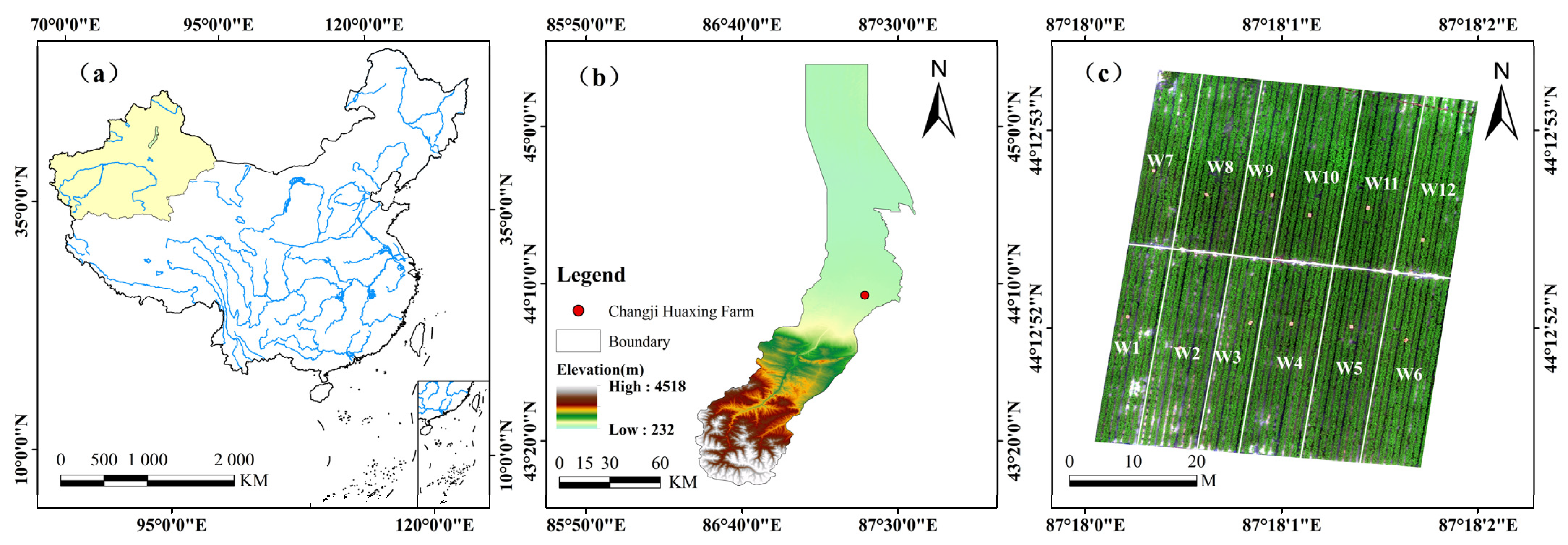
Figure 1. Overview map of the study area. (a) Location map of the study area; (b) elevation map of the Changji Huaxing Farm experimental area; (c) UAV image of the experimental plots.Note: The delineated boundaries represent the extent of the research region and do not necessarily reflect internationally recognized borders.
Agriculture 15 01815 g001
Figure 2. Meteorological data during the cotton growing season in 2023 (a) and 2024 (b).
Agriculture 15 01815 g002
Figure 3. Temporal variation of the first-order sensitivity index (FOSI) of aboveground biomass (AGB) for different crop parameters under 12 irrigation treatments (W1–W12) throughout the growing season. The x-axis represents days after sowing (DAS), the y-axis lists the crop parameters considered in the sensitivity analysis, and the color scale indicates the magnitude of the FOSI (0–1), where higher values denote a greater influence of the parameter on the model output.
Agriculture 15 01815 g003
Figure 4. Temporal variation of the total-order sensitivity index (TOSI) of aboveground biomass (AGB) for different crop parameters under 12 irrigation treatments (W1–W12) throughout the growing season. The x-axis represents days after sowing (DAS), the y-axis lists the crop parameters considered in the sensitivity analysis, and the color scale indicates the magnitude of the TOSI (0–1), where higher values denote a greater overall contribution of the parameter to the model output, including both its individual effect and interactions with other parameters.
Agriculture 15 01815 g004
Figure 5. Temporal variation of the first-order sensitivity index (FOSI) of canopy cover (CC) for different crop parameters under 12 irrigation treatments (W1–W12) throughout the growing season. The x-axis represents days after sowing (DAS), the y-axis lists the crop parameters considered in the sensitivity analysis, and the color scale indicates the magnitude of the FOSI (0–1), where higher values denote a greater influence of the parameter on the simulated CC.
Agriculture 15 01815 g005
Figure 6. Temporal variation of the total-order sensitivity index (TOSI) of canopy cover (CC) for different crop parameters under 12 irrigation treatments (W1–W12) throughout the growing season. The x-axis represents days after sowing (DAS), the y-axis lists the crop parameters considered in the sensitivity analysis, and the color scale indicates the magnitude of the TOSI (0–1), where higher values denote a greater overall contribution of the parameter to the simulated CC, including both its individual effect and interactions with other parameters.
Agriculture 15 01815 g006
Figure 7. Correlation analysis between vegetation indices and canopy cover (CC).Note: ** indicates significance at the p ≤ 0.01 level. The same notation applies hereinafter.
Agriculture 15 01815 g007
Figure 8. Relationship between remotely sensed and measured canopy cover (CC). Note: (ag) represent the CC inversions modeled by GNDVI, TVI, NBI, NDVI, NDRE, IPVI, and ridge regression, respectively.
Agriculture 15 01815 g008aAgriculture 15 01815 g008b
Figure 9. AGB inversion model (a) and model validation (b).
Agriculture 15 01815 g009
Figure 10. Fitness analysis of the Particle Swarm Optimization (PSO) algorithm.
Agriculture 15 01815 g010
Figure 11. Performance comparison radar charts before and after assimilation for 2023, 2024, and combined years (ALL). Evaluation metrics include the coefficient of determination (R2), root mean square error (RMSE), and index of agreement (d), which are compared for (a) canopy cover (CC), (b) aboveground biomass (AGB), and (c) yield (Y).
Agriculture 15 01815 g011
Figure 12. Relationship between total irrigation amount and cotton yield under different irrigation frequencies in different precipitation years. (a) Dry year; (b) normal year; (c) wet year.
Agriculture 15 01815 g012
Table 1. Irrigation treatment schemes used in the field experiment.
TreatmentP (Days/Time)Q (mm)TreatmentP (Days/Time)Q (mm)
W19405W47405
W2450W5450
W3495W6495
W75405W104405
W8450W11450
W9495W12495
Note: P is irrigation interval; Q is irrigation quota.
Table 2. Multispectral camera specifications and reflectance values of the calibration panel.
Band No.BandCentral Wavelength/
mm
Band Width/
mm
Calibration Panel Reflectance/
%
1Blue4753265
2Green5602763
3Red6681462
4Red Edge7171261
5Near-Infrared (NIR)8425760
Table 3. Grey relational degree between selected vegetation indices and AGB.
Vegetation
Index
Grey Relational Degrees Between Vegetation Indices and Aboveground Biomass (AGB)
Seedling
Stage
Budding
Stage
Flowering
Stage
Boll-Setting StageBoll-Opening Stage
NDVI0.640.840.840.840.70
SR0.710.740.710.740.45
SAVI0.660.840.840.840.70
EVI0.650.840.830.840.69
GNDVI0.660.830.840.830.70
NGRDI0.630.780.700.740.62
NPCI0.710.800.840.830.71
TVI0.650.810.830.830.69
VARI0.720.850.840.840.71
MSAVI0.650.840.840.840.70
OSAVI0.660.840.840.840.70
WDVI0.670.840.840.840.70
PSRI0.730.810.850.830.71
TCARI0.660.860.830.840.70
MCARI0.630.770.810.710.68
DVI0.670.840.840.840.70
IPVI0.640.820.830.830.70
MTVI0.640.830.830.840.70
NBI0.640.840.840.840.70
GCVI0.640.660.780.790.61
NDRE0.610.810.790.790.58
MSR0.590.690.630.660.69
Table 4. Linear relationships between CC and vegetation indices.
Vegetation
Index
Regression EquationR2RMSE (%)
GNDVIy = 0.328x + 0.5340.720.043
TVIy = 0.445x + 0.5920.690.046
NBIy = 0.224x + 0.5880.680.047
NDVIy = 0.224x + 0.5870.680.047
NDREy = 0.439x + 0.5920.670.047
IPVIy = 0.443x + 0.3680.670.047
Ridge Regressiony = 0.061 × GNDVI + 0.011 × IPVI − 0.035 × NBI + 0.011 × NDRE − 0.035 × NDVI + 0.057 × TVI + 0.7280.730.043
Note: x represents the corresponding vegetation index (VI); y represents the canopy cover (CC).
Table 5. Relationships between AGB and vegetation indices at different growth stages.
StageRegression EquationR2
(t·hm−2)
RMSE
(t·hm−2)
Seedling
Stage
y = −0.527 × PSRI − 0.232 × VARI − 0.009 × SR − 0.207 × NPCI + 0.194 × DVI + 2.9920.41 **1.03
Budding
Stage
y = 0.216 × PSRI − 0.057 × NPCI + 0.694 × VARI + 1.204 × GNDVI − 0.071 × OSAVI + 9.5410.97 **0.18
Flowering
Stage
y = 0.381 × VARI + 0.931 × TCARI + 0.273 × OSAVI + 0.326 × MSAVI − 0.947 × EVI + 5.6960.87 **0.38
Boll-Setting Stagey = 3.976 × MTVI + 1.467 × VARI − 0.317 × EVI − 3.868 × TCARI + 0.976 × MSAVI + 20.0210.71 **2.21
Boll-Opening Stagey = 0.144 × VARI − 1.402 × PSRI − 0.037 × NPCI + 2.189 × DVI − 1.811 × WDVI + 19.8620.46 **2.05
Note: y represents AGB, ** p < 0.01.
Table 6. Localized parameter values of the AquaCrop model.
NameParameter ValueRange
KCTRX1.20.72–1.5
CCS4.43.9–8.1
CSO4.23.9–8.1
CGC0.0750.05–0.1
CCX0.850.64–0.99
CDC0.070.02–0.08
WP2010.75–40.25
HI4032.5–67.5
SHI2519.5–40.5
Table 7. Linear regression results between observed and assimilated values.
State VariableYearSample SizeCC Regression
Equation
R2RMSE (%)d
PSOCC + AGB2023120y = 0.81x + 14.760.845.850.95
2024120y = 1.11x + 5.340.845.660.96
ALL240y = 0.96 + 4.980.845.760.96
YearSample SizeAGB Regression
Equation
R2RMSE (t·hm−2)d
2023120y = 0.97x + 0.260.951.630.98
2024120y = 0.96x + 0.250.951.570.98
ALL240y = 0.97x + 0.170.961.450.99
YearSample SizeYield Regression
Equation
R2RMSE (t·hm−2)d
202312y = 0.97x + 0.320.961.410.99
202412y = 0.96x + 0.480.951.400.98
ALL24y = 0.95x + 0.670.951.370.98
Table 8. Irrigation simulation scenarios under the AquaCrop model.
ScenarioSimulation SchemeIrrigation Quota/
mm
Irrigation Interval/
d
Number of IrrigationsTotal Irrigation Volume/
m3·hm−2
ScenarioSimulation SchemeIrrigation Quota/
mm
Irrigation Interval/
d
Number of IrrigationsTotal Irrigation Volume/
m3·hm−2
Scenario IP13304183300Scenario IIX1334185940
P23305153300X2335154950
P33307123300X3337123960
P4330993300X433992970
P54204184200X5424187560
P64205154200X6425156300
P74207124200X7427125040
P8420994200X842993780
P95104185100X9514189180
P105105155100X10515157650
P115107125100X11517126120
P12510995100X1251994590
Table 9. Simulation results of typical years under Scenario I with fixed irrigation quotas and varying irrigation frequencies.
Scenario I
Simulation SchemeDry YearNormal YearWet Year
YAGBWPETYAGBWPETYAGBWPET
P15.60 c16.96 c0.90 c491.83 a5.36 c15.95 c0.85 c509.33 b6.17 c18.31 c0.87 c522.33 c
P25.78 b17.75 b0.91 bc474.25 b5.55 b16.30 a0.86 c508.00 bc6.47 a18.51 b0.88 c522.00 c
P35.84 b18.21 b0.91 ab449.30 c5.62 bc16.46 ab0.90 b501.67 bc6.46 a18.45 b0.90 b523.83 b
P45.04 c17.26 c0.93 a491.83 c5.42 c16.09 bc0.90 b493.33 c6.22 b18.38 bc0.92 a524.33 a
P56.02 c19.33 c0.88 c542.17 a5.87 c19.23 c0.81 c575.83 b6.25 c20.07 c0.93 c572.33 c
P65.99 b19.64 b0.90 bc532.33 b6.15 b19.39 a0.83 c571.00 bc6.56 a20.46 b0.93 c581.33 c
P76.13 b20.26 b0.91 ab510.00 c6.01 bc20.04 ab0.85 b570.50 bc6.49 a20.38 b0.97 b582.50 b
P85.14 c18.88 c0.92 a490.62 c5.75 c18.12 bc0.86 b567.50 c6.35 b20.27 bc0.97 a586.17 a
P95.93 c19.23 c0.86 c558.33 a5.85 c17.46 c0.80 c619.17 b6.46 c21.18 c0.87 c606.33 c
P106.14 b19.74 b0.87 bc548.17 b6.06 b20.09 a0.81 c612.83 bc6.55 a21.33 b0.87 c606.83 c
P116.04 b19.60 b0.89 ab517.65 c5.83 bc18.13 ab0.83 b610.50 bc6.54 a21.32 b0.88 b610.50 b
P125.46 c19.28 c0.91 a514.02 c5.95 c19.37 bc0.83 b606.67 c6.51 b21.26 bc0.88 a609.67 a
Note: Different letters (a, b, c, ab, bc) indicate significant differences at the 0.05 level. Values with the same letter are not significantly different.
Table 10. Scenario 2: Simulation results of different irrigation frequencies under fixed irrigation quotas in different precipitation years.
Scenario II
Simulation SchemeDry YearNormal YearWet Year
YAGBWPETYAGBWPETYAGBWPET
X15.88 c18.32 c0.87 d524.25 a5.78 c18.31 c0.81 c608.17 a6.25 c17.46 d0.87 c608.67 a
X26.13 b19.77 b0.89 c514.55 ab6.10 b19.70 ab0.82 bc591.17 a6.49 b19.97 c0.87 c609.00 a
X36.13 b20.28 b0.93 b514.50 b6.14 b19.40 b0.87 b547.17 b6.48 b21.25 b0.93 b569.00 b
X45.02 b19.94 b0.94 a497.00 c5.91 b19.37 a0.90 a472.67 c6.61 b21.27 a0.98 a492.67 c
X55.86 c18.39 c0.86 d526.50 a5.65 c18.10 c0.81 c611.33 a6.49 c19.51 d0.87 c613.33 a
X66.08 b19.71 b0.88 c518.22 ab5.88 b18.28 ab0.83 bc609.00 a6.58 b21.45 c0.88 c613.33 a
X76.06 b19.71 b0.90 b516.35 b6.01 b19.45 b0.84 b607.83 b6.58 b21.45 b0.88 b609.00 b
X85.06 b19.94 b0.93 a512.00 c5.92 b19.39 a0.87 a545.50 c6.51 b21.28 a0.94 a554.83 c
X95.82 c17.65 c0.86 d545.00 a5.37 c15.39 c0.81 c630.00 a6.49 c20.88 d0.87 c621.33 a
X106.03 b18.95 b0.87 c538.92 ab5.83 b18.68 ab0.82 bc629.00 a6.66 b21.74 c0.88 c621.33 a
X115.96 b18.32 b0.88 b538.58 b5.80 b17.52 b0.83 b608.83 b6.64 b21.74 b0.88 b 609.50 b
X125.45 b18.85 b0.90 a524.70 c5.92 b19.29 a0.85 a578.33 c6.51 b21.26 a0.89 a597.17 c
Note: Different letters (a, b, c, ab, bc) indicate significant differences at the 0.05 level. Values with the same letter are not significantly different.
Disclaimer/Publisher’s Note: The statements, opinions and data contained in all publications are solely those of the individual author(s) and contributor(s) and not of MDPI and/or the editor(s). MDPI and/or the editor(s) disclaim responsibility for any injury to people or property resulting from any ideas, methods, instructions or products referred to in the content.